
Consistency Is Critical for the Effective Use of Baited Remote Video


1
College of Science, Swansea University, Wallace Building SA2 8PP, UK
2
Ocean Ecology Limited, River Office, Severnside Park, Epney GL2 7LN, UK
3
Department Life and Environmental Sciences, Faculty of Science and Technology, Bournemouth University, Christchurch House, Talbot Campus, Fern Barrow, Poole, Dorset BH12 5BB, UK
*
Author to whom correspondence should be addressed.
Oceans 2021, 2(1), 215-232; https://0-doi-org.brum.beds.ac.uk/10.3390/oceans2010013
Submission received: 21 December 2020
/
Revised: 23 February 2021
/
Accepted: 1 March 2021
/
Published: 3 March 2021
(This article belongs to the Special Issue ROVs and AUVs: New Technologies for the Future of Marine Research)
Abstract
:Baited remote underwater videos (BRUV) are popular marine monitoring techniques used for the assessment of motile fauna. Currently, most published studies evaluating BRUV methods stem from environments in the Southern Hemisphere. This has led to stricter and more defined guidelines for the use of these techniques in these areas in comparison to the North Atlantic, where little or no specific guidance exists. This study explores metadata taken from BRUV deployments collected around the UK to understand the influence of methodological and environmental factors on the information gathered during BRUV deployments including species richness, relative abundance and faunal composition. In total, 39 BRUV surveys accumulating in 457 BRUV deployments across South/South-West England and Wales were used in this analysis. This study identified 88 different taxa from 43 families across the 457 deployments. Whilst taxonomic groups such as Labridae, Gadidae and Gobiidae were represented by a high number of species, species diversity for the Clupeidae, Scombridae, Sparidae, Gasterosteidae and Rajidae groups were low and many families were absent altogether. Bait type was consistently identified as one of the most influential factors over species richness, relative abundance and faunal assemblage composition. Image quality and deployment duration were also identified as significant influential factors over relative abundance. As expected, habitat observed was identified as an influential factor over faunal assemblage composition in addition to its significant interaction with image quality, time of deployment, bait type and tide type (spring/neap). Our findings suggest that methodological and environmental factors should be taken into account when designing and implementing monitoring surveys using BRUV techniques. Standardising factors where possible remains key. Fluctuations and variations in data may be attributed to methodological inconsistencies and/or environment factors as well as over time and therefore must be considered when interpreting the data.
1. Introduction
Baited remote underwater videos (BRUV) are popular marine monitoring techniques used for the assessment of motile fauna [1]. Although these techniques have predominately focussed on fish assemblages [2], they have also been applied to large marine predators including sharks and pinnipeds as well as invertebrates such as cephalopoda and crustacea [1]. They have also been used for length measurements of assemblages, partcularly fish [1]. Such systems may consist of either one (mono) or two (stereo) cameras which film the area surrounding a bait used to attract motile fauna into the field of view of a camera [3,4,5]. Since the mid-1990s [6], these methods have been used to assess abundances, diversity and behaviour of motile assemblages [4,7,8] and have also been effective in aiding the assessment of metabolic rates [4]. They are a cost-effective and safer alternative to other methods such as underwater visual census, remotely operated vehicles or SCUBA divers where issues such as depth, submergence times and potentially dangerous fauna are considered limiting factors to data collection [9]. They are also considered a much less destructive alternative to extractive survey techniques such as benthic sediment grabbing and trawling [10].
Currently, most published studies evaluating BRUV methods stem from marine environments in the Southern Hemisphere with Australia and New Zealand leading leading the way in this research. Most assessments utilising BRUVs methods are undertaken on rocky reef, coral reef, and deep-water habitats [1]. Most assessments utilising BRUV methods are undertaken on rocky reef, coral reef and deep-water habitats [1] and in comparison relatively rarely on coastal soft-sediment habitats, although [11,12,13] provide more recent examples of such research. Studies have involved the use of various equipment set ups, bait types and sampling designs in varying environmental conditions.
Defined guidelines for BRUV methodologies in the North-Atlantic Region are currently lacking in comparison to countries such as New Zealand and Australia [14,15] where vertical and horizontal BRUV guidelines have been published. Recent reviews of the protocols associated with BRUV methodologies are now starting to pave the way globally for Findable, Accessible, Interoperable, and Reproducible (FAIR) workflows [16] when utilising these techniques [15]. Factors such as deployment duration [17], bait type [18,19,20,21], time of day [22,23], tidal currents [24] and habitat type [15,16,17,18,19,20,21,22,23,24,25] may influence information gathered for species richness, abundances, and faunal assemblage composition [26]. Within New Zealand for example, guidelines for BRUV deployments include important aspects such as descriptions of sources of bias (with suggestions of minimising and avoidance), sampling design, equipment, field deployment, data management, abundance and size estimates and data analysis [14]. This standardisation of methods is vital in monitoring biodiversity in a target area to ensure that comparisons between years or to other study locations is comprehensible and replicable in the future [24,27]. However, monitoring method guidelines are defined by the geographical area and policy areas which they serve [28]. Due to different biological (e.g., species and habitats) and environmental (e.g., hydrodynamics, sediments, topography) parameters present at different locations globally, a ‘one-method suits all’ approach may not be possible. Establishing and testing guidelines based on existing knowledge is therefore important for monitoring marine assemblages such as fish in different regions. Implementing such guidelines may allow for the effective management of protected areas to assess their effectiveness in conserving target biodiversity as well as allowing for future informed conservation decisions to be made for coastal developments [29].
This research explores metadata taken from a number of BRUV deployments collected between 2011 and 2018 from various habitats across South/South-West England and Wales, UK. Analysis identifies what species are recorded and absent using BRUV methods as well as explores the influences of methodological and environmental factors on species richness, relative abundance, and faunal composition. The aim of these findings is to provide an insight in to current BRUV methods used in coastal waters found around the North-Atlantic Region and provide a platform for the development of stricter, more consistent guidelines for the deployment of BRUVs.
2. Materials and Methods
2.1. Database Compilation
Data used for this research were taken from the archives of the following institutions: Swansea University; Ocean Ecology Limited; and Bournemouth University. These data were then supplemented with additional data collected between October 2017 and August 2018. In total, 39 BRUV surveys resulting in 457 BRUV deployments across South/South-West England and Wales (Figure 1) were compiled into one database for analysis.
For this study, relative abundance referred to the maximum number (MaxN) of individuals of a family or species present in any one frame of the video recorded. This measure has been extensively used in BRUV research [1] to avoid repeated counts of individuals [8,26].
The following key metadata were extracted from each deployment where available: habitat observed; time of deployment; bait type; duration of deployment (min); depth (m); image quality; tidal state/type; species richness; and relative abundance (MaxN).
The BRUV deployments targeted a variety of benthic habitats commonly found around the UK’s coastal waters including seagrass beds, sand, mixed course sediments and kelp beds and also used a variety of bait types including mackerel, squid, sardines, fish meal and prawn. Where access to the raw video footage was possible, deployments were categorised by time of day using the following criteria: dawn, day, evening, and night. Deployments undertaken in complete daylight or darkness were categorised as day and night, respectively, with deployments undertaken during the transitioning period from night to day and vice versa categorised as dawn and evening, respectively.
2.2. Image Quality Criteria
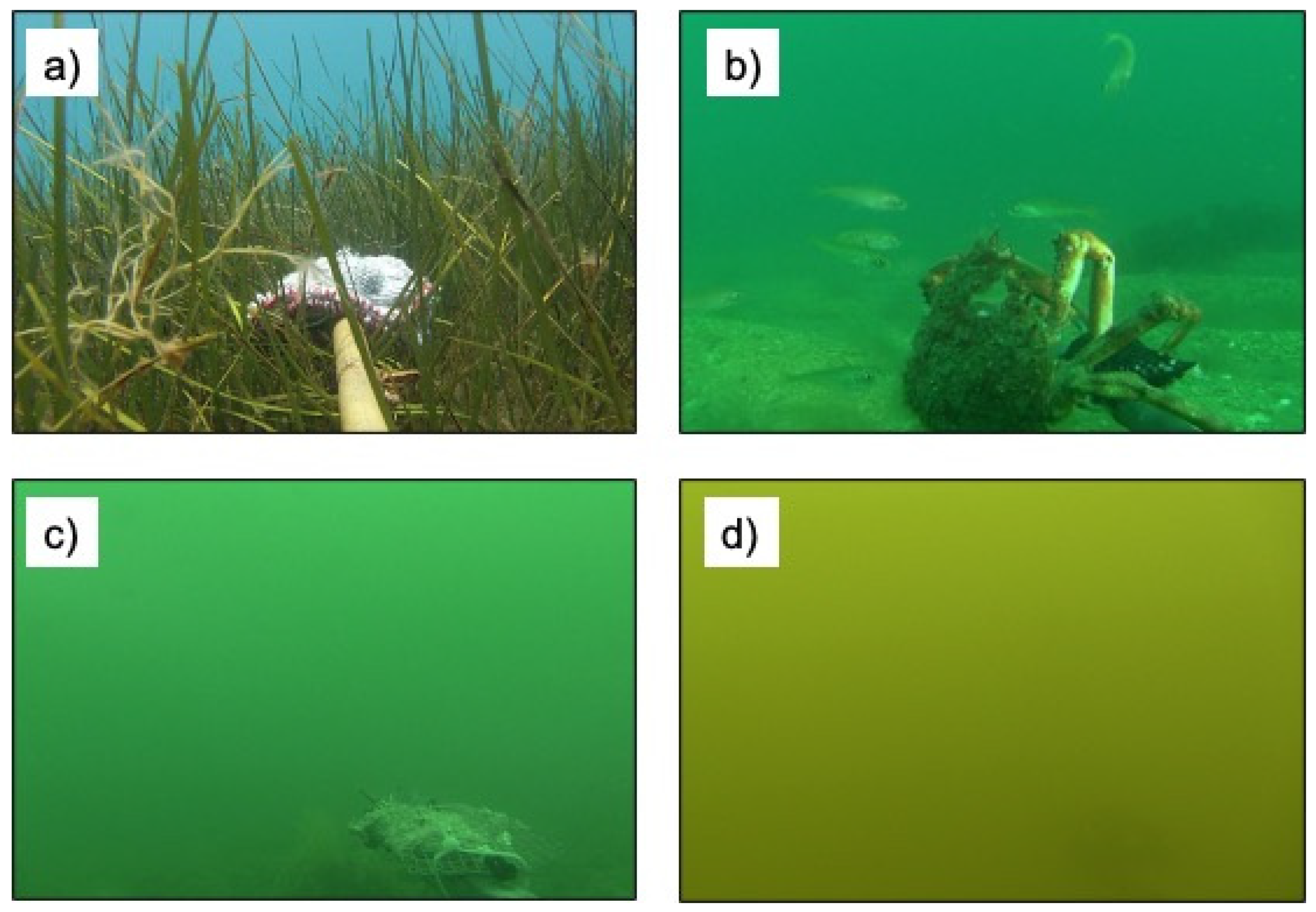
Defining the quality of BRUV footage is an important aspect when assessing the quality of information gathered by a deployment. Poor image quality may reduce the accuracy of identifying mobile species or render the footage unusable if deemed necessary. Table 1 presents the four categories used to determine BRUV image quality for this analysis with Figure 2 providing examples of these categories from the raw video footage compiled for this review.
2.3. Video Analysis
The majority of raw footage used in this analysis had already been processed for MaxN based on previous analytical methods used by Unsworth et al. (2014). Where footage was unprocessed, the same methodology was used. All fish assemblages and motile benthic macrofauna likely to be monitored in coastal habitats using BRUV methods were included in this analysis. Taxa were identified to the highest level possible depending on the visibility of distinguishable features. Organisms were identified as unknown if turbidity levels affected confidence of identification.
Prior to analysis, raw footage was compressed from Advanced Video Coding High-Definition (AVCHD) format (standard format for digital recordings and high-definition video camcorders) to Audio Video Interleave (AVI) format using Xilisoft Video Converter Ultimate for use in the specialist SeaGIS software Event Measure.
2.4. Data Analysis
Univariate analyses were conducted using RStudio (Version 4.0.0) and Minitab (Version 11). Significant results were considered p ≤ 0.05 and all means reported ± 1 Standard Error (SE). Where data were unobtainable, cells were left blank. The following categorical predictors were assessed: habitat observed, image quality, time of day, bait type, tide type (spring/neap), tidal state (high to low, low to high) and slack tide (yes or no). Depth was not used in this analysis due to the low number of BRUV deployments recording it as metadata. Categorical predictors were coded (1,0) with reference levels for the categorical predictors with more than two levels as follows: Broad-scale habitat = sand, image quality = excellent, time of day = day, bait type = none, spring/neap tide = mid. Duration of deployment was included as a continuous predictor in this assessment.
Species richness and relative abundance (MaxN) were square root transformed prior to analysis to reduce variance heterogeneity. Generalised linear models using a Poisson regression (family = poisson, link = log) were fitted to evaluate the influence of BRUV categorical predictors. Prior to running the models, we examined whether there was multicollinearity between any of the predictors based on the variance inflation factor (VIF) using the ‘car’ package in R. An aliased test was also carried out to identify which variables were linearly dependent on others (subsequently causing perfect multicollinearity). Based on this test, the slack tide predictor variable was removed as it was shown to be highly correlated with tidal state for both species richness and relative abundance. Once removed, the remaining seven predictors all presented VIF values < 3 [30]. A base model was initially created using the seven remaining predictors. A stepwise regression following a sequential replacement was then used to find the subset of variables resulting in the best-performing model. A chi-square goodness of fit test was used to determine how well the theoretical distribution fit the empirical distribution.
Multivariate analysis on faunal assemblage composition was undertaken on square root-transformed species data using PRIMER-e v7 plus PERMANOVA+ software [31]. Bray–Curtis dissimilarity matrices (including a dummy variable to deal with deployments with no fauna) were created prior to conducting statistical analyses and visualised using non-metric multidimensional scaling (nMDS) plots. Following this, a two-way permutational multivariate analysis of variance (PERMANOVA) [32] was used to test for interactions between habitat observed and the remaining categorical predictors on faunal assemblage composition. These tests were based on 9999 unrestricted permutations of the raw data with significant results considered p ≤ 0.01. Pairwise comparisons were subsequently run on the significant interactions between the habitat observed and the categorical predictors identified by the PERMANOVA. Two-way similarity percentage (SIMPER) analyses were used to identify the main species recorded on the BRUVs responsible for any differences between habitat observed and the significant interactions between the remaining categorical predictors identified in the PERMANOVA.
3. Results
3.1. General Observations
Out of the 457 BRUV deployments used in this assessment, 16 were subject to low visibility (4%), 13 toppled due to strong currents (3%) and 5 failed due to a camera fault (1%) totalling 34 failed deployments.
Access to raw footage of 147 deployments was unavailable (32%). The image quality of these was therefore classified as N/A. Of the remaining deployments, 52 were considered excellent image quality (11%), 106 considered good image quality (23%), 133 considered poor image quality (29%) and 19 were considered unusable (4%), 16 of which were due to excessive low visibility conditions where the bait was not visible. Duration of deployments all ranged from 10 to 360 min; 75% of BRUV deployments were 60 min.
Nine habitats were targeted across the 457 deployments; 25 BRUV deployments were located on artificial reefs (6%), 2 on chalk reefs (<1%), 42 in kelp (9%), 33 in midwater (7%), 37 on mixed coarse sediments (8%), 2 on mussel beds (<1%), 25 on rocky reefs (6%), 158 on sand (35%) and 130 in seagrass (28%). Habitat data were unavailable for three deployments (<1%) and were therefore classed as N/A. For time of day, 290 BRUV deployments were undertaken during daylight hours (64%), 19 were undertaken at night (4%), 16 were undertaken at dawn (4%) and 42 were undertaken in the evening (9%). Times of day were unavailable for 90 deployments; these were therefore classified as N/A (19%).
Across all deployments, seven bait types were utilised: 16 used crab (4%), 244 used mackerel (53%), 35 used no bait (8%), 39 used oily fish meal (9%), 11 used prawn (2%), 3 used sardines (1%) and 34 used squid (7%). Data were unavailable for 75 deployments and were therefore classified N/A (16%).
For tide type, 106 BRUV deployments were undertaken during spring tides (23%), 115 undertaken during mid tides (25%) and 95 were on neap tides (21%). Deployment dates were unavailable for 141 deployments and were therefore classified as N/A (31%). The tidal state was considered as running high to low for 74 deployments (16%), low to high for 76 deployments (17%) with 307 classified as N/A (67%). Out of the 457 deployments, 47 were undertaken on slack tide (10%) with 103 not (23%) and 307 classified as N/A (67%).
In total, 88 different taxa from 43 families were recorded throughout the 39 BRUV surveys (Supplementary Information Table S1). Lesser spotted dogfish (Scyliorhinus canicula) was recorded within 113 BRUV deployments across all surveys with the two-spotted goby Gobiusculus flavescens also recorded in a high number of deployments at 93. Out of the 43 families recorded across all surveys, those highest represented by different species were Labridae, Gadidae and Gobiidae with six species each. A number of families were notably represented by a lower number of species, these included Clupeidae, Scombridae, Sparidae, Soleidae, Gasterosteidae and Rajidae with one species each. Cryptic (morphologically indistinguishable) species such as those from the Syngnathidae were difficult to identify to species level. Pelagic and mid-water species were not recorded in high numbers during the 457 BRUV deployments used in this research.
3.2. Species Richness
Following a stepwise regression analysis, only one predictor, bait type was identified in the best-performing generalised linear model (family = poisson) for species richness during BRUV deployments with an R2 value of 26.09% and AIC value of 328.64 (Table 2). A chi-square goodness of fit test for this model returned p = 1.00, suggesting that there is no evidence that the data do not follow a Poisson distribution.
Observations of the coefficients within the bait predictor (Supplementary Material, Section B, Table S2) showed that oily fish meal and fish oils (1.160, p ≤ 0.001) and mackerel (0.830, p = 0.006) had the largest positive influences over species richness in BRUV deployments compared to unbaited deployments (Figure 3d).
3.3. Relative Abundance
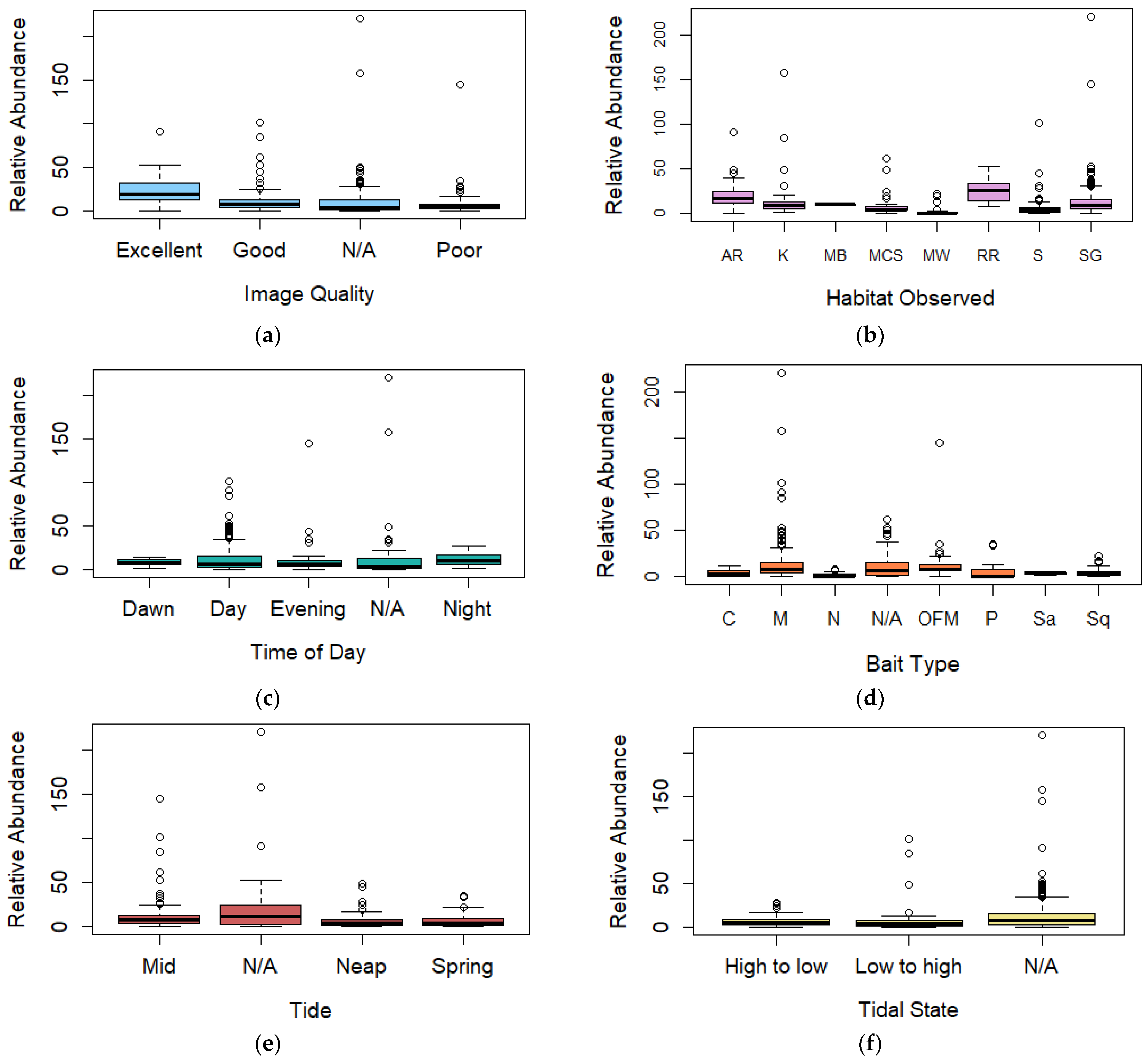
Following a stepwise regression analysis, three predictors—bait type, image quality and deployment duration—were included in the best-performing generalised linear model (family = poisson) for relative abundance during BRUV deployments with an R2 value of 36.70% and an AIC value of 416.61 (Table 3). A chi-square goodness of fit test for this model returned p = 0.849, suggesting that there is no evidence that the data do not follow a Poisson distribution.
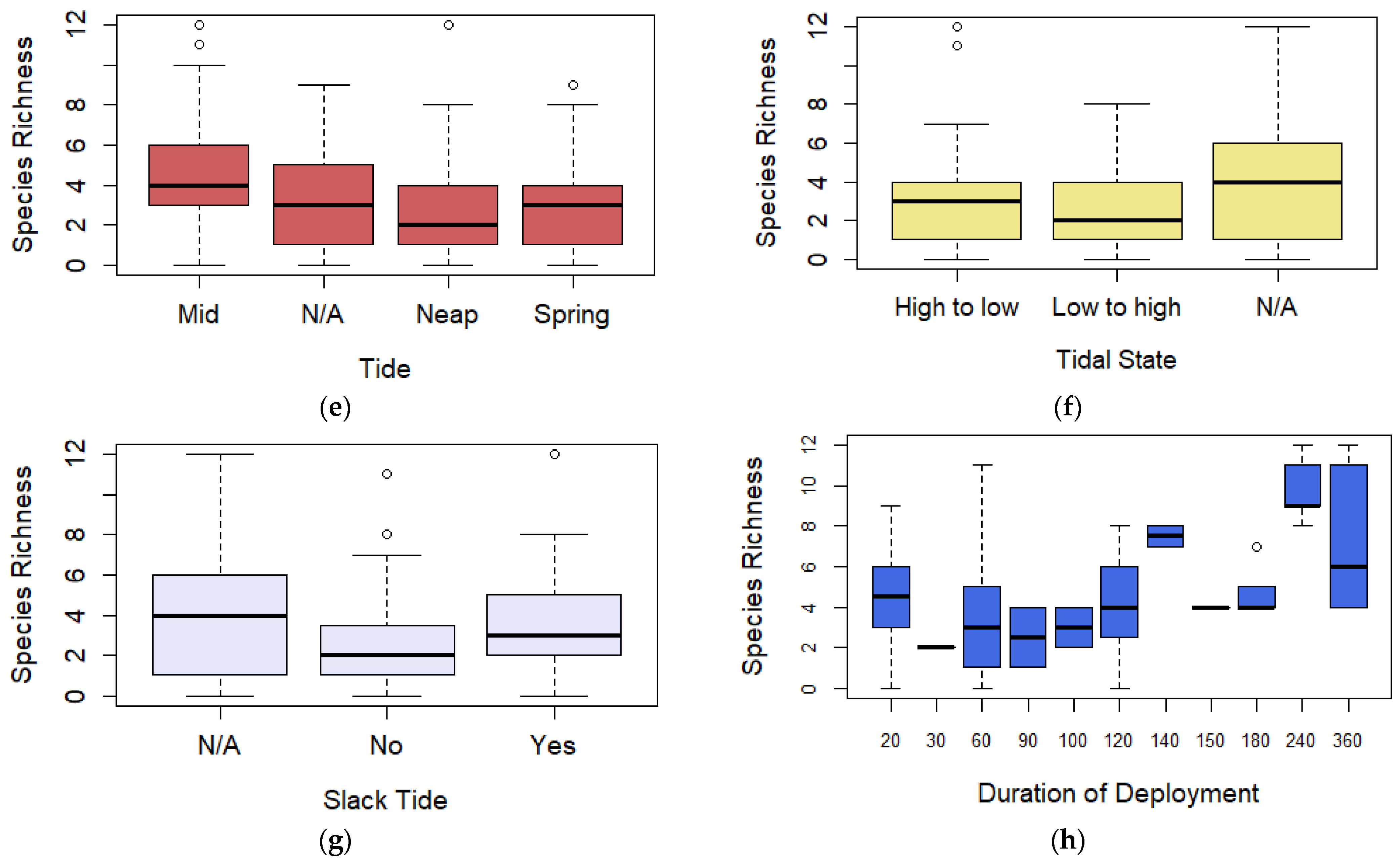
Observations of the coefficients for the three predictors are presented in the Supplementary Material, Section B, Table S3. For the image quality predictor, coefficients showed that deployments recording a poor image quality had a larger negative influence (−0.894, p = 0.032) compared to deployments of excellent image quality (Figure 4a). For the bait predictor, coefficients again showed that oily fish meal and fish oils (0.992, p = 0.003) and mackerel (0.970, p ≤ 0.001) had the largest positive influences over relative abundance BRUV deployments compared to unbaited deployments (Figure 4d). Duration of deployment was also found to have a positive effect over relative abundance (p = 0.003) (Figure 4h).
3.4. Faunal Assemblage Composition
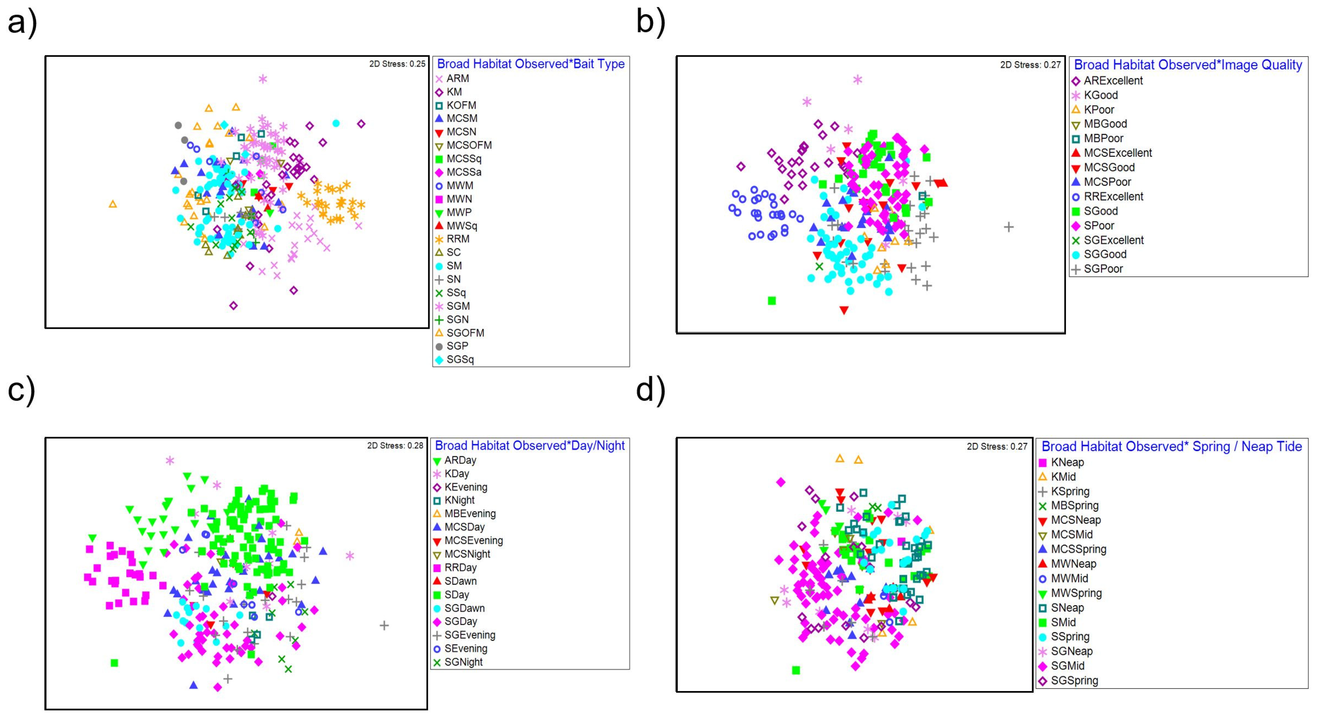
A PERMANOVA test of faunal assemblage composition identified significant influences of deployment time of day, bait type and tide (spring/mid/neap) on faunal assemblage composition and their interaction with habitat observed. In addition to this, a significant interaction was also present between the habitat observed and image quality. No significant effects or interactions were observed for tidal state and slack tide on faunal assemblage composition across BRUV deployments (Figure 5; Table 4).
Pairwise comparisons (Supplementary Material, Section C, Table S4) for the interaction between habitat observed and image quality identified significant differences in faunal assemblage composition between poor and good image qualities within sand (t = 1.8104, p = 0.003) and seagrass habitats (t = 2.896, p ≤ 0.001). A SIMPER analysis (Supplementary Material, Section D, Table S5) identified the following taxa Gobiidae, Paguridae and Scyliorhinus canicula as the highest contributors (cumulative 30.70%) to differences between poor and good image qualities. Furthermore, unidentifiable individuals were also recorded in higher abundances in poor image qualities also contributing to these differences.
For the interaction between habitat observed and deployment time of day, pairwise comparisons presented significant differences in faunal assemblage composition between day and evening deployments (t = 2.0880, p ≤ 0.001) within sand habitat. Further differences were also identified between day and evening (t = 2.0439, p ≤ 0.001), day and dawn (t = 2.4133, p ≤ 0.001), day and night (t = 2.2477, p ≤ 0.001) and dawn and night (t = 3.3442, p ≤ 0.001) BRUV deployments within seagrass habitats. Differences between day and night (t = 2.0131, p = 0.003) within kelp habitats were also observed. A SIMPER analysis identified abundances of the following species Atherina presbyter, Gobiusculus flavescens and Ammodytidae as the main contributors to differences in faunal composition.
Pairwise comparisons for the interaction between habitat observed and bait type identified significant differences in faunal composition between mackerel and unbaited deployments within mixed coarse sediments (t = 1.7949, p = 0.001), sand (t = 2.9881, p = <0.001), seagrass (t = 2.3400, p ≤ 0.001) and midwater habitats (t = 2.3687, p ≤ 0.010). Differences were also identified between mackerel and squid (t = 2.0463, p ≤ 0.001) mackerel and crab (t = 1.9546, p = 0.001) squid and no bait (t = 2.1969, p ≤ 0.001) and crab and no bait (t = 2.0300, p = 0.009) deployments within sand habitats. Differences in faunal assemblage composition between mackerel and oily fish meal were also observed within seagrass (t = 3.8963, p ≤ 0.001) and kelp (t = 2.3184, p ≤ 0.001) habitats. Furthermore, differences between oily fish meal and no bait (t = 2.4533, p ≤ 0.001) prawn (t = 2.1780, p ≤ 0.001) and squid (t = 1.9675, p = 0.001) were observed in seagrass habitats. A SIMPER analysis identified abundances of Gobiidae, Scyliorhinus canicula, Paguridae and Merlangius merlangius as the species most contributing differences between bait types.
Except for midwater habitats, pairwise comparisons presented a significant interaction for faunal assemblage composition between habitat observed and tide (spring/mid/neap) (Table 4). Within mixed coarse sediment and seagrass habitats, differences in composition were observed between all tide types (Supplementary Material, Section C, Table S4). Within sand habitats, differences in faunal composition were observed between spring and mid (t = 2.3531, p ≤ 0.001) and neap and mid tides (t = 2.2792, p ≤ 0.001). Similarly, differences between spring and mid tides were observed within kelp habitats (t = 2.0015, p = 0.007). A SIMPER analysis identified abundances of Gobiidae, Scyliorhinus canicula, Paguridae and Merlangius merlangius as the species most contributing differences between tides.
4. Discussion
This study provides a unique quantitative assessment of the methodological and environmental factors influencing information collected using BRUV systems in a northern temperate environment. It provides an important validation of recent reviews of BRUV protocols [15] and will help direct sampling design when implementing BRUV assessments in the North-Atlantic Region.
Our study identified that BRUV techniques are very good tools for sampling taxonomic groups such as Labridae, Gadidae and Gobiidae. However, our findings also suggest that these techniques may be less suitable for sampling families such as Clupeidae, Scombridae, Sparidae, Gasterosteidae and Rajidae. Furthermore, morphologically indistinguishable species (cryptic) also become lost when implementing these tools. Seasons should be considered when interpreting data from BRUV deployments, especially across years as these may also influence the species present as well as relative abundances in any one deployment [33]. Of the nine habitats targeted during the 457 BRUV deployments, only 7% were conducted in midwater habitats. With the underrepresentation of pelagic species across surveys, further research into the implementation of midwater BRUVs in the UK would give a better insight into their applicability for monitoring these species. As it stands, most BRUV systems have been designed to target demersal fish species, manipulating them to be deployed in the water column may improve their use in targeting pelagic/mid water fish assemblages.
Bait type was consistently identified as the most influential factor over species richness, relative abundance, and faunal assemblage composition. Out of the 457 BRUV deployments considered in this study, 244 (53%) used mackerel as bait, suggesting that this is a favoured bait across different institutions in the UK. Previous BRUV studies globally have also favoured oily fish bait types [1] and have also found it to be the best-performing when undertaking experimental comparisons to unbaited deployments [5,18,19,34]. Our findings also identify similar patterns with mackerel and oily fish meal having a significant positive influence over species richness and relative abundance in UK coastal waters compared to unbaited deployments. Furthermore, the amount of bait has also previously been noted in past research as influencing diversity and abundance recordings during BRUV deployments and wider techniques such as traps utilising bait [35,36,37]. Any methodological inconsistencies in BRUV sampling designs must therefore be considered when implementing these methods with regards to the type and amount of bait used. The standardisation of bait use across the UK is a key factor for recording consistent ecological data over time, especially for monitoring and comparison surveys which span years over a specific area [21]. Changes to bait type used may in itself influence diversity, abundance and composition data recorded. In addition to bait type, deployment duration was also found as having an influence over relative abundance. Similar results have been identified through past research conducted in coastal habitats in the North- Atlantic Region [17] where minimum deployment times of 1 and 2 h are required to sample 66% and 83% of fish species, respectively.
Image quality was a significant negative influence on data collection, with only 52 (12%) deployments classed as excellent quality in comparison to 133 (29%) deployments classified as poor quality. The low number of excellent-quality images in the study was attributed to the dynamic environments associated with the UK. For instance, large tidal ranges, wave energy [38] and seabed currents [39] all influence large amounts of sediment transport in the water column [38] in turn reducing underwater visibility. Determining when BRUV footage is useable or not is important in understanding the quality and accuracy of data recorded. At present, there are no strict guidelines on what can be classified as a useable BRUV deployment. In this study, deployments where the camera system toppled into the sediment obscuring field of view, were subject to high levels of turbidity or had a fault during deployment was classified as an unusable deployment. The classification of high turbidity levels reducing image quality was measured by visualising whether the bait was visible during the video recording. Previous camera studies have found that increased turbidity levels can greatly reduce data accuracy [3,40]. A potential solution to reducing the impacts of image quality when comparing BRUV deployments in low visibility environments could be to standardise the field of view when using stereo BRUVs or other low technology methods. This would allow for high-quality and low-quality images to be more comparable. For example, if the lowest useable visibility is 1 m, excluding videos with visibility under that and standardise everything else to 1 m by only analysing fish that are within 1 m of cameras (relative abundance and species richness) in all footage (including high-quality images).
In our study, lower abundances of benthic prey species such as Gobiidae in poor-quality images were identified as influencing differences in faunal assemblage composition within sand and seagrass habitats. In contrast to this, scavenging species, such as Scyliorhinus canicula and Paguridae were recorded in high abundances in lower-quality images, suggesting that these individuals are more likely to approach the bait during deployments in high turbidity. When analysing poor-quality image footage, we must consider that scavenging species are more likely to approach the bait when compared to smaller benthic prey species which may be located at a distance from the bait but still attracted to the wider plume [20,41]. Recent improvements in BRUV image clarity using clear liquid optical chambers [9] also provide a practical alternative in low visibility conditions, expanding the working window for BRUV methods.
The habitats targeted for BRUV deployments included both soft-sediments habitats such as sand and seagrass as well as hard substrates such as rocky and artificial reefs. Contrary to initial thoughts, habitat was not identified as the most important factor influencing species richness and relative abundance during this study. However, as expected, faunal assemblage composition was heavily influenced by the habitat in which the BRUV was deployed in. Tide type and deployment time of day were also observed as having an effect over faunal composition. Past studies have identified similar effects of diurnal and tidal variation on assemblage abundances and composition in habitats such as mud and sandflats associated with estuarine environments [42], saltmarsh creeks [43] as well as tropical tidal flats [44]. Observations or measurements of currents and tidal state during BRUV deployments should be recorded where possible as metadata as these can affect the bait plume area and potentially result in different conclusions when comparing to other datasets if these factors are not considered [24]. It was noted during this study that of the 34 failed deployments recorded, 24 (71%) occurred during spring tides where the camera footage was unable to be analysed either due to toppling into the sediment or subject to high levels of turbidity. Suspended sediment matter tends to be higher during spring tides compared to neap and mid tides limiting underwater visibility, especially around soft-sediment coastal and estuarine environments [45,46,47]. Furthermore, tidal currents also tend to be stronger during spring tides [48] increasing the likelihood of the camera system toppling. It is therefore recommended that deploying BRUVs during spring tides should be avoided.
Although this study provides a unique overview of BRUV methods in the North-Atlantic region, it has highlighted the need for comprehensive metadata to be obtained during these surveys for BRUV datasets to be more comparable. During this research, it became apparent that the level of detail in the metadata attributed to each BRUV deployment varied. For example, bait weight, tidal state, season, water temperature, and approximate distance to other habitats should be included in metadata records but was not something consistently recorded in these datasets. Deploying BRUVs within soft-sediment habitats in close proximity to other habitats such as reefs can influence halo effects. Fetterplace [49] has suggested that BRUVs should be deployed a minimum of 200 m from reef habitats when sampling soft-sediment communities as a standardised means of avoiding such halo effects [50]. For this research, assumptions were made that all bait types used were the same weight for comparisons to be made. Although past research has suggested that bait weight may not always influence relative abundance, species richness or faunal assemblage composition recorded in BRUV deployments in the North-Atlantic region [21], this information is still an aspect which should be recorded as metadata and remain consistent when designing surveys using these tools.
5. Conclusions
Our findings give an insight into methodological and environmental factors which should be considered when designing and implementing BRUV techniques and have highlighted the need for comprehensive and consistent metadata to be collected during each survey for accurate data comparisons. Fluctuations and variations in data may be attributed to methodological inconsistencies and/or environmental factors as well as over time or due to anthropogenic influences and therefore must be considered when analysing and interpreting the data.
Although BRUV techniques are a repeatable, cost-effective, non-destructive, widely used method, a full evaluation into whether they are suitable or designed for the individuals being targeted must be undertaken. The quality and state of the environment in which they are being deployed in must also be considered prior to conducting surveys using these tools.
Supplementary Materials
The following are available online at https://0-www-mdpi-com.brum.beds.ac.uk/2673-1924/2/1/13/s1.
Author Contributions
Conceptualisation, R.K.F.U. and R.A.G.; Methodology, R.K.F.U., R.A.G., and R.E.J.; Formal Analysis, R.E.J.; Investigation, R.E.J.; Resources, R.K.F.U., R.A.G., R.J.H.H. and R.E.J.; Data Curation, R.E.J.; Writing—Original Draft Preparation, R.E.J.; Writing—Review and Editing, R.K.F.U., R.J.H.H. and R.A.G.; Visualisation, R.E.J.; Supervision, R.K.F.U. and R.A.G.; Project Administration, R.K.F.U.; Funding Acquisition, R.K.F.U. and R.J.H.H. All authors have read and agreed to the published version of the manuscript.
Funding
This work was supported by the Knowledge Economy Skills Scholarships 2. This is a pan-Wales higher level skills initiative led by Bangor University on behalf of the higher education sector in Wales. It is funded by the Welsh Government’s European Social Fund convergence programme for West Wales and the Valleys. Support and funding were also given by the European Union Regional Development Fund through the SEACAMS 2 project in Swansea University. Support and funding were also given to R.J.H.H. from Esmée Fairbairn Foundation and Bournemouth Borough Council.
Data Availability Statement
Restrictions apply to the availability of these data. Data was obtained from Swansea University, Bournemouth University and Ocean Ecology and are available from the authors with the permission of these three institutions.
Acknowledgments
Firstly, we acknowledge the time and effort of many individuals who collected the original datasets at Swansea University, Ocean Ecology and Bournemouth University. We would also like to acknowledge the support and funding given by Knowledge Economy Skills Scholarships (KESS). We would also like to acknowledge the support and funding given by Ocean Ecology Ltd. and EU ERDF funding through the SEACAMS 2 project.
Conflicts of Interest
The authors declare no conflict of interest.
References
- Whitmarsh, S.K.; Fairweather, P.G.; Huveneers, C. What is Big BRUVver up to? Methods and uses of baited underwater video. Rev. Fish Biol. Fish. 2017, 27, 53–73. [Google Scholar] [CrossRef]
- Lowry, M.; Folpp, H.; Gregson, M.; Mckenzie, R. A comparison of methods for estimating fish assemblages associated with estuarine artificial reefs. Braz. J. Oceanogr. 2011, 59, 119–131. [Google Scholar] [CrossRef]
- Mallet, D.; Pelletier, D. Underwater video techniques for observing coastal marine biodiversity: A review of sixty years of publications (1952–2012). Fish. Res. 2014, 154, 44–62. [Google Scholar] [CrossRef]
- Cappo, M.; Harvey, E.S.; Shortis, M. Counting and Measuring Fish with Baited Video Techniques—An Overview. In Proceedings of the Australian Society for Fish Biology Workshop Proceedings, Hobart, Australia, 28–29 August 2006; pp. 101–114. [Google Scholar] [CrossRef]
- Wraith, J.; Lynch, T.; Minchinton, T.E.; Broad, A.; Davis, A.R. Bait type affects fish assemblages and feeding guilds observed at baited remote underwater video stations. Mar. Ecol. Prog. Ser. 2013, 477, 189–199. [Google Scholar] [CrossRef] [Green Version]
- Ellis, D.M.; DeMartini, E.E. Evaluation of a video camera technique for indexing abundances of juvenile pink snapper, Pristipomoides filamentosus, and other Hawaiian insular shelf fishes. Fish. Bull. 1995, 93, 67–77. [Google Scholar]
- Martinez, I.; Jones, E.G.; Davie, S.L.; Neat, F.C.; Wigham, B.D.; Priede, I.G. Variability in behaviour of four fish species attracted to baited underwater cameras in the North Sea. Hydrobiologia 2011, 670, 23–34. [Google Scholar] [CrossRef]
- Priede, I.G.; Ragley, P.M.; Smith, K.L. Seasonal change in activity of abyssal demersal scavenging grenadiers Coryphaenoides (Nematonums) armatus in the eastern North Pacific Ocean. Limnol. Oceanogr. 1994, 39, 279–285. [Google Scholar] [CrossRef]
- Jones, R.E.; Griffin, R.A.; Rees, S.C.; Unsworth, R.K. Improving visual biodiversity assessments of motile fauna in turbid aquatic environments. Limnol. Oceanogr. Methods 2019, 17, 544–554. [Google Scholar] [CrossRef] [Green Version]
- Davies, J.; Baxter, J.; Bradley, M.; Connor, D.; Khan, J.; Murray, E.; Sanderson, W.; Turnbull, C.; Vincent, M. Marine Monitoring Handbook; Joint Nature Conservation Committee: Peterborough, UK, 2001; ISBN 1 86107 5243.
- Borland, H.; Schlacher, T.; Gilby, B.; Connolly, R.; Yabsley, N.; Olds, A. Habitat type and beach exposure shape fish assemblages in the surf zones of ocean beaches. Mar. Ecol. Prog. Ser. 2017, 570, 203–211. [Google Scholar] [CrossRef] [Green Version]
- Schultz, A.L.; Malcolm, H.A.; Ferrari, R.; Smith, S.D. Wave energy drives biotic patterns beyond the surf zone: Factors influencing abundance and occurrence of mobile fauna adjacent to subtropical beaches. Reg. Stud. Mar. Sci. 2019, 25, 100467. [Google Scholar] [CrossRef]
- Vargas-Fonseca, E.; Olds, A.D.; Gilby, B.L.; Connolly, R.M.; Schoeman, D.S.; Huijbers, C.M.; Hyndes, G.A.; Schlacher, T.A. Combined effects of urbanization and connectivity on iconic coastal fishes. Divers. Distrib. 2016, 22, 1328–1341. [Google Scholar] [CrossRef] [Green Version]
- Haggitt, T.; Freeman, D.; Lily, C. Baited Remote Underwater Video Guidelines; eCoast Ltd.: Raglan, New Zealand, 2014; p. 82. [Google Scholar]
- Langlois, T.; Goetze, J.; Bond, T.; Monk, J.; Abesamis, R.A.; Asher, J.; Barrett, N.; Bernard, A.T.F.; Bouchet, P.J.; Birt, M.J.; et al. A field and video annotation guide for baited remote underwater stereo-video surveys of demersal fish assemblages. Methods Ecol. Evol. 2020, 11, 1401–1409. [Google Scholar] [CrossRef]
- Wilkinson, M.D.; Dumontier, M.; Aalbersberg, I.J.; Appleton, G.; Axton, M.; Baak, A.; Blomberg, N.; Boiten, J.-W.; da Silva Santos, L.B.; Bourne, P.E.; et al. Comment: The FAIR Guiding Principles for scientific data management and stewardship. Sci. Data 2016, 3, 1–9. [Google Scholar] [CrossRef] [PubMed] [Green Version]
- Unsworth, R.; Peters, J.; McCloskey, R.; Hinder, S. Optimising stereo baited underwater video for sampling fish and invertebrates in temperate coastal habitats. Estuar. Coast. Shelf Sci. 2014, 150, 281–287. [Google Scholar] [CrossRef]
- Dorman, S.R.; Harvey, E.S.; Newman, S.J. Bait Effects in Sampling Coral Reef Fish Assemblages with Stereo-BRUVs. PLoS ONE 2012, 7, e41538. [Google Scholar] [CrossRef] [Green Version]
- Hannah, R.W.; Blume, M.T.O. The Influence of Bait and Stereo Video on the Performance of a Video Lander as a Survey Tool for Marine Demersal Reef Fishes in Oregon Waters. Mar. Coast. Fish. 2014, 6, 181–189. [Google Scholar] [CrossRef] [Green Version]
- Harvey, E.S.; Cappo, M.; Butler, J.J.; Hall, N.; Kendrick, G.A. Bait attraction affects the performance of remote underwater video stations in assessment of demersal fish community structure. Mar. Ecol. Prog. Ser. 2007, 350, 245–254. [Google Scholar] [CrossRef] [Green Version]
- Jones, R.E.; Griffin, R.A.; Januchowski-Hartley, S.R.; Unsworth, R.K. The influence of bait on remote underwater video observations in shallow-water coastal environments associated with the North-Eastern Atlantic. PeerJ 2020, 8, e9744. [Google Scholar] [CrossRef]
- Bassett, D.; Montgomery, J. Investigating nocturnal fish populations in situ using baited underwater video: With special reference to their olfactory capabilities. J. Exp. Mar. Biol. Ecol. 2011, 409, 194–199. [Google Scholar] [CrossRef]
- Birt, M.J.; Harvey, E.S.; Langlois, T.J. Within and between day variability in temperate reef fish assemblages: Learned response to baited video. J. Exp. Mar. Biol. Ecol. 2012, 416–417, 92–100. [Google Scholar] [CrossRef]
- Taylor, M.D.; Baker, J.; Suthers, I.M. Tidal currents, sampling effort and baited remote underwater video (BRUV) surveys: Are we drawing the right conclusions? Fish. Res. 2013, 140, 96–104. [Google Scholar] [CrossRef]
- McLean, D.L.; Langlois, T.J.; Newman, S.J.; Holmes, T.H.; Birt, M.J.; Bornt, K.R.; Bond, T.; Collins, D.L.; Evans, S.N.; Travers, M.J.; et al. Distribution, abundance, diversity and habitat associations of fishes across a bioregion experiencing rapid coastal development. Estuar. Coast. Shelf Sci. 2016, 178, 36–47. [Google Scholar] [CrossRef]
- Grimmel, H.M.; Bullock, R.W.; Dedman, S.L.; Guttridge, T.L.; Bond, M.E. Assessment of faunal communities and habitat use within a shallow water system using non-invasive BRUVs methodology. Aquac. Fish. 2020, 5, 224–233. [Google Scholar] [CrossRef]
- Costello, M.J.; Basher, Z.; Mcleod, L.; Asaad, I.; Claus, S.; Vandepitte, L.; Yasuhara, M.; Gislason, H.; Edwards, M.; Appeltans, W.; et al. The GEO Handbook on Biodiversity Observation Networks; Springer: Berlin/Heidelberg, Germany, 2017. [Google Scholar] [CrossRef] [Green Version]
- Turrell, W. Improving the implementation of marine monitoring in the northeast Atlantic. Mar. Pollut. Bull. 2018, 128, 527–538. [Google Scholar] [CrossRef] [PubMed]
- Murphy, H.M.; Jenkins, G.P. Observational methods used in marine spatial monitoring of fishes and associated habitats: A review. Mar. Freshw. Res. 2010, 61, 236–252. [Google Scholar] [CrossRef]
- Zuur, A.; Ieno, E.N.; Elphick, C.S. A protocol for data exploration to avoid common statistical problems. Methods Ecol. Evol. 2010, 1, 3–14. [Google Scholar] [CrossRef]
- Clarke, K.R.; Gorley, R.N. Primer V6: User Manual—Tutorial; Plymouth Marine Laboratory: Plymouth, UK, 2007. [Google Scholar] [CrossRef] [Green Version]
- Anderson, M.J. Permutational Multivariate Analysis of Variance (PERMANOVA); Wiley StatsRef: Statistics Reference Online; John Wiley & Sons, Ltd.: Chichester, UK, 2017; pp. 1–15. [Google Scholar] [CrossRef]
- Sherman, C.S.; Heupel, M.R.; Johnson, M.; Kaimuddin, M.; Qamar, L.M.S.; Chin, A.; Simpfendorfer, C.A. Repeatability of baited remote underwater video station (BRUVS) results within and between seasons. PLoS ONE 2020, 15, e0244154. [Google Scholar] [CrossRef]
- Bernard, A.T.F.; Götz, A. Bait increases the precision in count data from remote underwater video for most subtidal reef fish in the warm-temperate Agulhas bioregion. Mar. Ecol. Prog. Ser. 2012, 471, 235–252. [Google Scholar] [CrossRef] [Green Version]
- Cyr, C.; Sainte-Marie, B. Catch of Japanese crab traps in relation to bait quantity and shielding. Fish. Res. 1995, 24, 129–139. [Google Scholar] [CrossRef]
- Miller, R.J. How Many Traps Should a Crab Fisherman Fish? N. Am. J. Fish. Manag. 1983, 3, 1–8. [Google Scholar] [CrossRef]
- Hardinge, J.; Harvey, E.S.; Saunders, B.J.; Newman, S.J. A little bait goes a long way: The influence of bait quantity on a temperate fish assemblage sampled using stereo-BRUVs. J. Exp. Mar. Biol. Ecol. 2013, 449, 250–260. [Google Scholar] [CrossRef]
- Pattiaratchi, C.; Collins, M. Sediment transport under waves and tidal currents: A case study from the northern Bristol Channel, U.K. Mar. Geol. 1984, 56, 27–40. [Google Scholar] [CrossRef]
- Heathershaw, A.; Langhorne, D. Observations of near-bed velocity profiles and seabed roughness in tidal currents flowing over sandy gravels. Estuar. Coast. Shelf Sci. 1988, 26, 459–482. [Google Scholar] [CrossRef]
- O’Byrne, M.; Schoefs, F.; Pakrashi, V.; Ghosh, B. An underwater lighting and turbidity image repository for analysing the performance of image-based non-destructive techniques. Struct. Infrastruct. Eng. 2017, 14, 104–123. [Google Scholar] [CrossRef] [Green Version]
- Whitmarsh, S.K.; Huveneers, C.; Fairweather, P.G. What are we missing? Advantages of more than one viewpoint to estimate fish assemblages using baited video. R. Soc. Open Sci. 2018, 5, 171993. [Google Scholar] [CrossRef] [PubMed] [Green Version]
- Morrison, M.A.; Francis, M.P.; Hartill, B.W.; Parkinson, D.M. Diurnal and Tidal Variation in the Abundance of the Fish Fauna of a Temperate Tidal Mudflat. Estuar. Coast. Shelf Sci. 2002, 54, 793–807. [Google Scholar] [CrossRef]
- Hampel, H.; Cattrijsse, A.; Vincx, M. Tidal, diel and semi-lunar changes in the faunal assemblage of an intertidal salt marsh creek. Estuar. Coast. Shelf Sci. 2003, 56, 795–805. [Google Scholar] [CrossRef]
- Reis-Filho, J.A.; Barros, F.; Nunes, J.; Sampaio, C.L.S.; De Souza, G.B.G. Moon and tide effects on fish capture in a tropical tidal flat. J. Mar. Biol. Assoc. UK 2011, 91, 735–743. [Google Scholar] [CrossRef]
- Grabemann, I.; Uncles, R.; Krause, G.; Stephens, J. Behaviour of Turbidity Maxima in the Tamar (U.K.) and Weser (F.R.G.) Estuaries. Estuar. Coast. Shelf Sci. 1997, 45, 235–246. [Google Scholar] [CrossRef]
- Uncles, R.J. Physical properties and processes in the Bristol Channel and Severn Estuary. Mar. Pollut. Bull. 2010, 61, 5–20. [Google Scholar] [CrossRef]
- Allen, G.; Salomon, J.; Bassoullet, P.; Du Penhoat, Y.; de Grandpré, C. Effects of tides on mixing and suspended sediment transport in macrotidal estuaries. Sediment. Geol. 1980, 26, 69–90. [Google Scholar] [CrossRef]
- Gonzalez-Santamaria, R.; Zou, Q.-P.; Pan, S. Impacts of a Wave Farm on Waves, Currents and Coastal Morphology in South West England. Estuaries Coasts 2013, 38, 159–172. [Google Scholar] [CrossRef]
- Fetterplace, L. The Ecology of Temperate Soft Sediment Fishes: Implications for Fisheries Management and Marine Protected Area Design. Ph.D. Thesis, University of Wollongong, Wollongong, Australia, 2017. Available online: https://ro.uow.edu.au/theses1/375 (accessed on 23 February 2021).
- Schultz, A.L.; Malcolm, H.A.; Bucher, D.J.; Smith, S.D.A. Effects of Reef Proximity on the Structure of Fish Assemblages of Unconsolidated Substrata. PLoS ONE 2012, 7, e49437. [Google Scholar] [CrossRef] [PubMed] [Green Version]
Figure 1.
Map showing the locations of the BRUV surveys which form the database used in this analysis.
Figure 1.
Map showing the locations of the BRUV surveys which form the database used in this analysis.
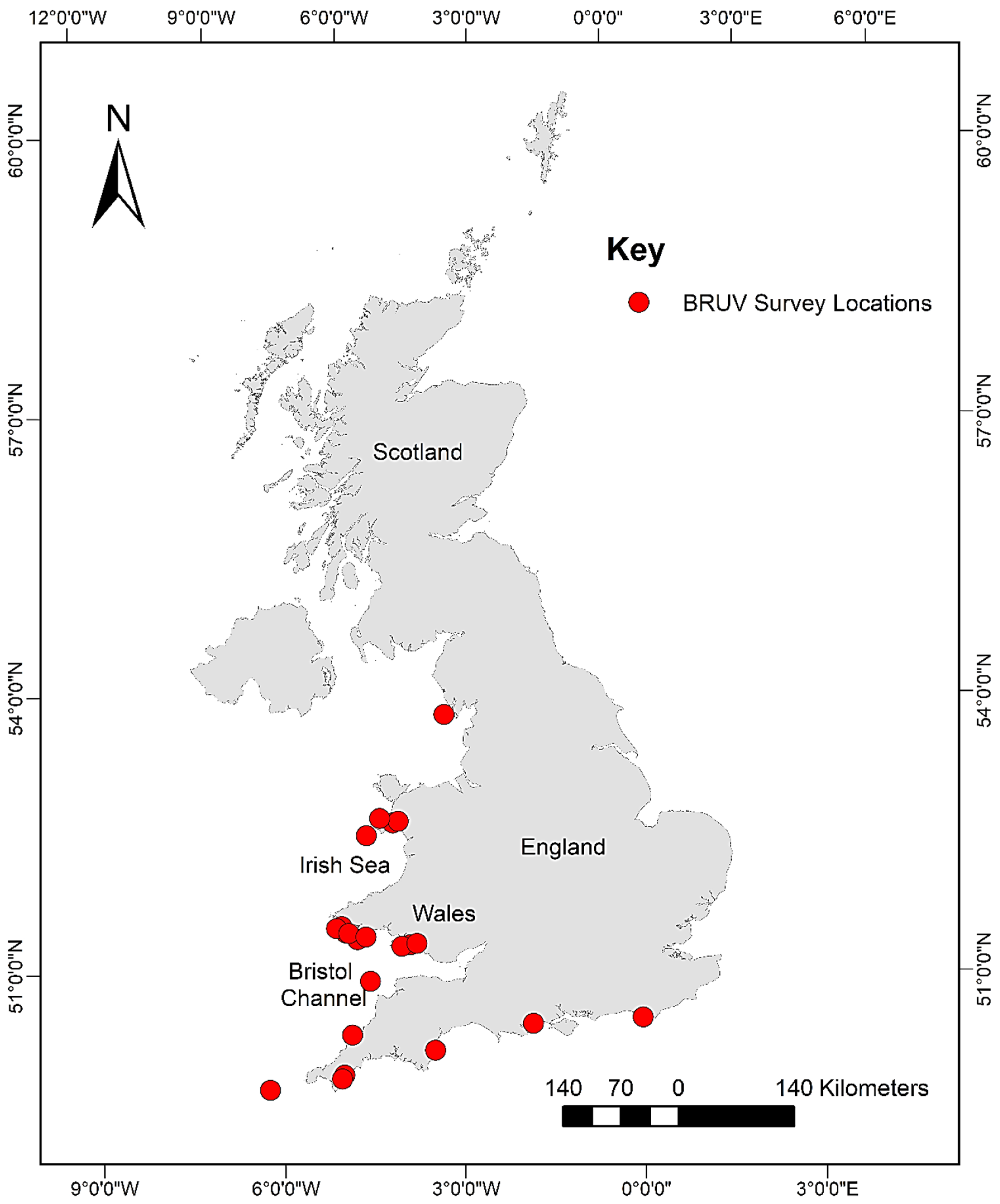
Figure 2.
Examples of the image quality criteria used in developing the BRUV database: (a) excellent, (b) good, (c) poor and (d) unusable.
Figure 2.
Examples of the image quality criteria used in developing the BRUV database: (a) excellent, (b) good, (c) poor and (d) unusable.

Figure 3.
Boxplot (box ranging from first to third quartile and highlighting median value, whiskers extending to 1.5 the interquartile distance with circles indicating outliers) comparing species richness for (a) image quality, (b) broad habitat observed, (c) time of day, (d) bait type, (e) spring/neap tides, (f) tidal state, (g) slack tide, and (h) duration of deployment. AR = Artificial Reef, K = Kelp, MB = Mussel Beds, MCS = Mixed Coarse Sediment, MW = Midwater, RR = Rocky Reef, S = Sand, SG = Seagrass, C = Crab, M = Mackerel, OFM = Oily fish meal and fish oils, N = No bait, P = Prawn, Sa = Sardines, and Sq = Squid.
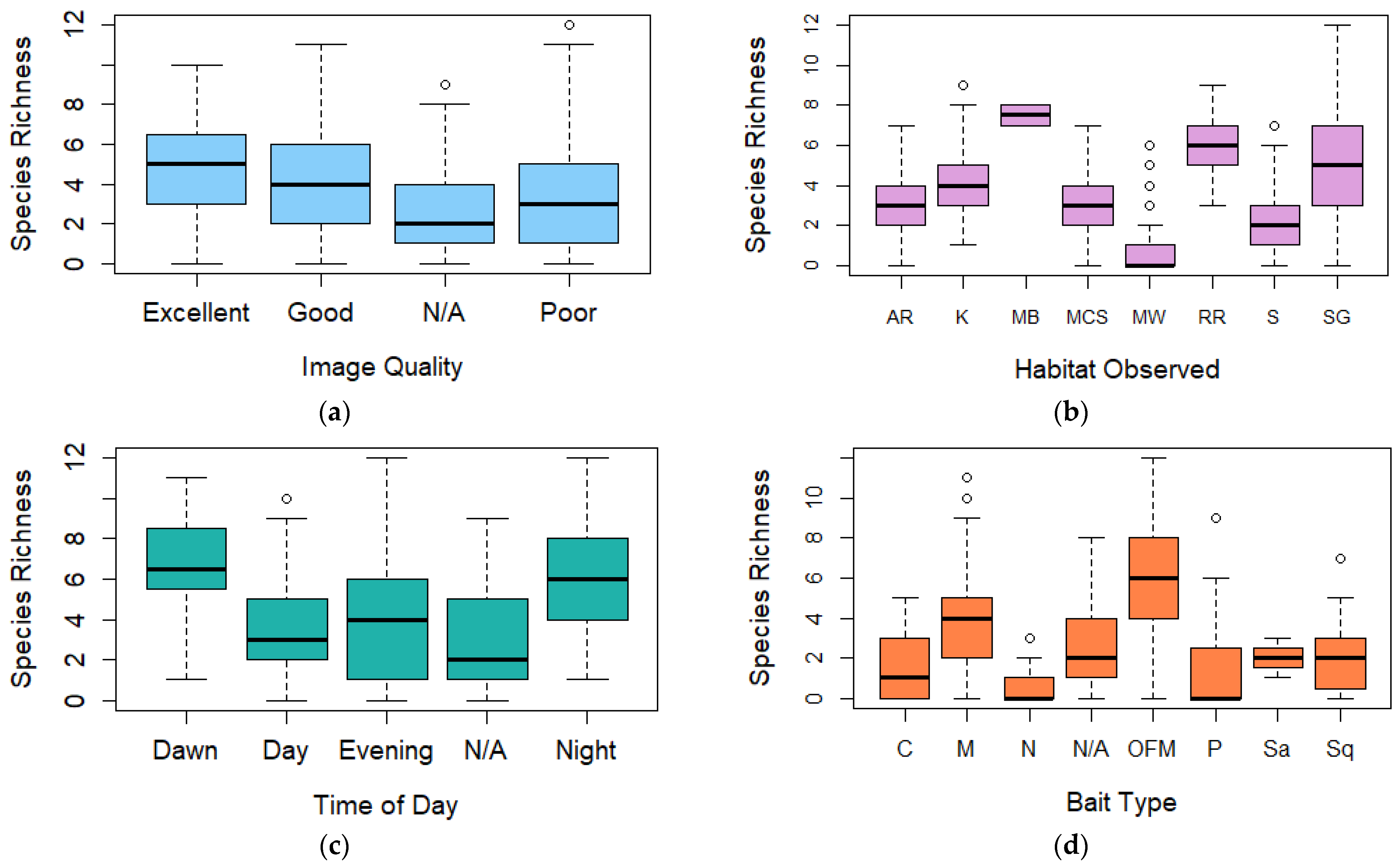

Figure 4.
Boxplot (box ranging from first to third quartile and highlighting median value, whiskers extending to 1.5 the interquartile distance with circles indicating outliers) comparing relative abundance for (a) image quality, (b) broad habitat observed, (c) time of day, (d) bait type, (e) spring/neap tides, (f) tidal state, (g) slack tide, and (h) duration of deployment. AR = Artificial Reef, K = Kelp, MB = Mussel Beds, MCS = Mixed Coarse Sediment, MW = Midwater, RR = Rocky Reef, S = Sand, SG = Seagrass, C = Crab, M = Mackerel, OFM = Oily fish meal and fish oils, N = No bait, P = Prawn, Sa = Sardines, and Sq = Squid.


Figure 5.
nMDS plot for interactions between (a) broad habitat observed and bait type, (b) broad habitat observed and image quality, (c) broad habitat observed and time of day, and (d) broad habitat observed and spring/neap tide. AR = Artificial Reef, K = Kelp, MCS = Mixed Coarse Sediment, MW = Midwater, RR = Rocky Reef, S = Sand, SG = Seagrass, C = Crab, M = Mackerel, OFM = Oily fish meal and fish oils, N = No bait, Sa = Sardines, Sq = Squid, and P = Prawn.


Table 1.
Image quality criteria categories, code and description for BRUV footage in compiled database.
Table 1.
Image quality criteria categories, code and description for BRUV footage in compiled database.
| Image Category | Image Code | Description |
|---|---|---|
| Excellent | 3 | Can clearly see the bait plus over 1 m into the distance. |
| Good | 2 | Can clearly see the bait and maximum 1 m into the distance. |
| Poor | 1 | Can see the bait only. |
| Unusable | 0 | Unable to see bait and fish not clearly visible for identification purposes. |
Table 2.
Best-performing models assessing what predictors have the most influence over species richness during BRUV deployments based on AIC values. Note N/A has been excluded from this statistical analysis.
Table 2.
Best-performing models assessing what predictors have the most influence over species richness during BRUV deployments based on AIC values. Note N/A has been excluded from this statistical analysis.
| Predictors | AIC | AICc | R2 |
|---|---|---|---|
| Base model: All 7 predictors | 346.05 | 352.45 | 35.68% |
| Bait Type | 328.64 | 329.34 | 26.09% |
| Bait Type + Tidal State | 330.62 | 331.57 | 26.11% |
| Bait Type + Tidal State + Image Quality | 331.43 | 332.99 | 30.76% |
| Broad Habitat + Bait Type + Tidal State | 333.06 | 334.97 | 31.30% |
| Bait Type + Tidal State + Spring/Neap | 334.23 | 335.79 | 26.68% |
| Habitat Observed + Bait Type + Tidal State + Duration | 334.31 | 336.62 | 32.40% |
| Habitat Observed + Bait Type + Tidal State + Spring/Neap + Duration | 334.69 | 336.60 | 28.92% |
| Habitat Observed + Bait Type + Tidal State + Image Quality | 335.44 | 338.20 | 33.66% |
| Habitat Observed + Bait Type + Tidal State + Spring/Neap | 336.82 | 339.58 | 31.65% |
| Habitat Observed + Bait Type + Tidal State + Image Quality + Duration | 336.82 | 340.07 | 34.56% |
| Habitat Observed + Bait Type + Tidal State + Time of Day | 338.79 | 342.04 | 31.69% |
| Duration + Tidal State | 339.68 | 339.87 | 11.92% |
| Habitat Observed + Bait Type + Tidal State + Time of Day + Duration | 340.11 | 343.89 | 32.69% |
| Habitat Observed + Bait Type + Tidal State + Time of Day +Image Quality | 341.06 | 345.43 | 34.21% |
| Habitat Observed + Bait Type + Tidal State + Time of Day + Image Quality + Duration | 342.51 | 347.50 | 35.01% |
Table 3.
Best-performing models assessing what predictors have the most influence over relative abundance (MaxN) during BRUV deployments based on AIC values. Note* N/A has been excluded from this statistical analysis.
Table 3.
Best-performing models assessing what predictors have the most influence over relative abundance (MaxN) during BRUV deployments based on AIC values. Note* N/A has been excluded from this statistical analysis.
| Predictors | AIC | AICc | R2 |
|---|---|---|---|
| Base model: All 7 predictors | 426.66 | 433.05 | 41.67% |
| Bait Type + Image Quality + Duration | 416.61 | 418.16 | 36.70% |
| Bait Type + Image Quality + Duration + Tidal State | 418.61 | 420.52 | 36.71% |
| Bait Type + Image Quality + Duration + Tidal State + Spring/Neap | 420.35 | 423.11 | 38.12% |
| Bait Type + Image Quality + Duration + Tidal State + Habitat Observed | 421.65 | 424.90 | 38.56% |
| Bait Type + Image Quality + Duration + Tidal State + Time of Day | 422.56 | 425.81 | 37.99% |
| Bait Type + Image Quality + Duration + Tidal State + Spring/Neap + Habitat Observed | 423.25 | 427.62 | 40.05% |
| Bait Type + Image Quality + Duration + Tidal State + Time of Day + Spring/Neap | 423.61 | 427.97 | 39.83% |
Table 4.
PERMANOVAs for faunal assemblage composition assessing the influence of the six categorical predictors during BRUV deployments and their interaction with habitat observed. * Note N/A has been excluded from this statistical analysis Bold values p ≤ 0.01.
Table 4.
PERMANOVAs for faunal assemblage composition assessing the influence of the six categorical predictors during BRUV deployments and their interaction with habitat observed. * Note N/A has been excluded from this statistical analysis Bold values p ≤ 0.01.
| Source | df | MS | Pseudo-F | P(Perm) | Unique Perms |
|---|---|---|---|---|---|
| Habitat Observed * Image Quality | |||||
| Habitat Observed | 6 | 19,518 | 9.969 | <0.001 | 9806 |
| Image Quality | 2 | 2361.7 | 1.2012 | 0.1965 | 9897 |
| Hab * Image | 5 | 5241.2 | 2.6656 | <0.001 | 9838 |
| Residual | 270 | 1966.2 | |||
| Total | 283 | ||||
| Habitat Observed * Time of Day | |||||
| Habitat Observed | 6 | 25,071 | 12.65 | <0.001 | 9830 |
| Time of Day | 3 | 4899.5 | 2.4721 | <0.001 | 9858 |
| Hab * Time | 6 | 4212.4 | 2.1254 | <0.001 | 9816 |
| Residual | 317 | 1981.9 | |||
| Total | 332 | ||||
| Habitat Observed * Bait Type | |||||
| Habitat Observed | 7 | 25,553 | 14.634 | <0.001 | 9809 |
| Bait Type | 7 | 6663.6 | 3.8161 | <0.001 | 9801 |
| Hab * Bait | 8 | 6049.2 | 3.4643 | <0.001 | 9807 |
| Residual | 325 | 1746.2 | |||
| Total | 347 | ||||
| Habitat Observed * Tide (Spring/Neap) | |||||
| Habitat Observed | 5 | 14,915 | 7.5186 | <0.001 | 9847 |
| Tide | 2 | 6924.2 | 3.4906 | <0.001 | 9903 |
| Hab * Tide | 8 | 6849.6 | 3.4530 | <0.001 | 9820 |
| Residual | 267 | 1983.7 | |||
| Total | 282 | ||||
| Habitat Observed * Tidal State | |||||
| Habitat Observed | 4 | 10,272 | 5.2581 | <0.001 | 9885 |
| Tidal State | 1 | 2601.9 | 1.3319 | 0.2148 | 9921 |
| Hab * State | 3 | 1721.7 | 0.88133 | 0.6547 | 9896 |
| Residual | 119 | 1953.5 | |||
| Total | 127 | ||||
| Habitat Observed * Slack Tide | |||||
| Habitat Observed | 4 | 14,867 | 7.6298 | <0.001 | 9862 |
| Slack Tide | 1 | 2831.9 | 1.4533 | 0.1518 | 9928 |
| Hab*Slack | 3 | 2584.9 | 1.3266 | 0.1177 | 9915 |
| Residual | 119 | 1948.5 | |||
| Total | 127 |
Publisher’s Note: MDPI stays neutral with regard to jurisdictional claims in published maps and institutional affiliations. |
© 2021 by the authors. Licensee MDPI, Basel, Switzerland. This article is an open access article distributed under the terms and conditions of the Creative Commons Attribution (CC BY) license (http://creativecommons.org/licenses/by/4.0/).
Share and Cite
MDPI and ACS Style
Jones, R.E.; Griffin, R.A.; Herbert, R.J.H.; Unsworth, R.K.F. Consistency Is Critical for the Effective Use of Baited Remote Video. Oceans 2021, 2, 215-232. https://0-doi-org.brum.beds.ac.uk/10.3390/oceans2010013
AMA Style
Jones RE, Griffin RA, Herbert RJH, Unsworth RKF. Consistency Is Critical for the Effective Use of Baited Remote Video. Oceans. 2021; 2(1):215-232. https://0-doi-org.brum.beds.ac.uk/10.3390/oceans2010013
Chicago/Turabian StyleJones, Robyn E., Ross A. Griffin, Roger J. H. Herbert, and Richard K. F. Unsworth. 2021. "Consistency Is Critical for the Effective Use of Baited Remote Video" Oceans 2, no. 1: 215-232. https://0-doi-org.brum.beds.ac.uk/10.3390/oceans2010013