Influence of the Seasonal Thermocline on the Vertical Distribution of Larval Fish Assemblages Associated with Atlantic Bluefin Tuna Spawning Grounds

Abstract

Temperature is often an important variable influencing the vertical position of fish larvae in the water column. The same species may show different vertical distributions in areas with a strong near-surface seasonal thermocline compared to isothermal near-surface regions. In areas with a strong surface thermocline, tuna larvae show a significant preference for the near-surface warmer layers. Little is known regarding larval tuna vertical distribution in isothermal waters and on the vertical distribution of the associated larval fish assemblages. We conducted vertical stratified sampling using the same methodology and fishing device (MOCNESS) in the two major spawning areas of Atlantic bluefin tuna (BFT): western Mediterranean Sea (MED), characterized by a surface thermocline, and the Gulf of Mexico (GOM) which lacks thermal stratification. Tuna larvae occupied the upper 30 m in both areas, but the average larval depth distribution was consistently deeper in the GOM. In the MED, vertical distribution of larval fish assemblages was explained by temperature, and species such as BFT, Thunnus alalunga, and Ceratoscopelus maderensis, among others, coexist above the thermocline and are separated from species such as Cyclothone braueri and Hygophum spp. (found below the thermocline). In the GOM, the environmental correlates of the vertical distribution of the larvae were salinity and fluorescence. Mesopelagic taxa such as Ceratoscopelus spp. and Cyclothone spp., among others, had a shallower average distribution than Lampanyctus spp., Hygophum spp., and Myctophum spp.

1. Introduction

Biodiversity, ecosystem functioning, and abiotic factors are interrelated [1]. Communities can be dominated by a few species with particular traits or by complementary species that are differently adapted to the habitat [1,2]. The habitat frames relationships among species. The species composition of marine fish larval communities has been usually related to habitats in the “horizontal” dimension (e.g., the spatial distribution of species regarding abiotic variables [3]). However, significant physical, chemical, and biological gradients in the vertical dimension of the water column influence the vertical distribution of fish larvae. The place where a larva is relative to these gradients profoundly influences the development and success of the larval phase. The horizontal advection of fish larvae from spawning to nursery areas also depends on the vertical position of the larvae in the water column [4]. In general, the presence or absence of persistent clines in the open ocean can influence the vertical distribution and composition of larval fish assemblages [5].

There has been an historical interest describing the species composition in tuna assemblages due to their economic and ecological importance as top predators. Juvenile and adult tuna species dominate in particular areas worldwide and separate niches across their vertical distribution when coexisting [6,7]. Early in their life cycle, a variety of tuna species coexist in most spawning grounds worldwide with particular species dominating in the different areas [8,9,10,11]. Temperature arises as a key variable explaining the presence of tuna larvae in all areas [12,13,14,15,16,17]. As such, temperature is one primary variable explaining the worldwide distribution of major tuna spawning areas [18,19] and recruitment variability [20]. Other environmental variables such as salinity and fluorescence explain larval spatial segregation of tuna species at a small spatial scale [8,14,21,22,23].

In contrast to the adult stage, niche segregation of tuna species with depth and companion species during the early life stages has been little studied. Atlantic bluefin tuna (BFT), as with other tuna species, reproduce in temperatures above 20 °C conducive for survival and development of eggs and larvae [24,25]. Therefore, temperature is often the primary variable used to explain the shallow depth distribution of tuna larvae in environments with a strong seasonal thermocline where temperatures of 20 °C occur at around 20 m depth (e.g., Pacific bluefin tuna in the Nansei area [26]; Albacore and BFT in the NW Mediterranean [27]). However, tunas also reproduce in areas that lack a strong near-surface seasonal thermocline and where temperatures above 20 °C are mixed throughout the upper water column. Within these locations, little is known about the vertical distribution of tuna larvae [9]. Pacific bluefin tuna larvae, Thunnus orientalis, is the only species for which the vertical distribution has been compared across two spawning areas with different scenarios showing a shallower and narrower distribution in areas with a strong thermocline [28]. Laboratory experiments show that BFT and bonito larvae occupy a wider depth range when temperatures are vertically homogeneous compared to when waters are stratified, in which case BFT larvae are confined to the surface mixed layer [27]. Vertical temperature distributions may then play a major role on the vertical distribution of tuna species and companion species, a task that has received little attention in the literature.

Among the different spawning areas for BFT and other tuna species, the Gulf of Mexico (GOM) in the western Atlantic and the western Mediterranean Sea (MED) in the eastern Atlantic are the ones with a longer time series of annual samplings to study the horizontal distribution of larval fish assemblages, although using different methodologies [22]. Integrated sampling has been conducted from the surface down to the 70 m depth in the MED [29,30,31,32] and from the surface down to 200 m depth in the GOM [33]. In both areas, BFT coexists with other tuna species: Thunnus atlanticus, T. albacares, T. obesus, Auxis spp., Euthynnus spp., and Katsuwonus spp., and the horizontal assemblages are dominated mainly by mesopelagic larvae. For both areas, increasing densities of tuna larvae have been reported since 2010; however, which taxa are increasing differs: BFT in the MED [34] and Thunnus spp. in the GOM [33]. Differences in these integrated sampling methodologies make the comparison between assemblages difficult and further complicate the understanding of vertical processes that could enhance our understanding of the ecological role of bluefin tuna larvae in the larval fish community.

The BFT spawning season comprises April to June in the GOM and June to July in the MED [22]. In both spawning areas the horizontal larval habitat is characterized by warm waters [22]; however, water column properties differ between the areas [9]. The vertical distribution of chlorophyll during the BFT spawning periods is similar in both areas, with maximum chlorophyll concentrations occurring around 80–90 m depth [9]. Although salinity values are higher in the MED than in the GOM, the water column is isohaline in both sites, which is typical of open ocean waters [9]. In contrast, the thermal stratification differs between the two spawning areas with a strong thermocline at 20 m in the MED and a deeper thermocline around 100 m in the GOM [9]. Comparison of the water column properties in these two areas can help us understand how the thermal structure of the water column influences larval fish ecology and community structure.

Until now, no comparable data on the vertical distribution of BFT and the associated larval assemblages has been available. No studies have examined in detail how environmental conditions influence the vertical distribution of BFT larvae and their associated ichthyoplankton community in either the GOM or the MED. If temperature remains the primary variable explaining the vertical distributions of larvae, then we would expect tuna larvae to be found more deeply distributed in isothermal areas than in those that are thermally stratified. The aim of this study was: (1) to test the influence of thermal stratification on the vertical distributions of larval tuna, and (2) to determine whether the association between the vertical distributions of larval fish assemblages in BFT spawning grounds is influenced by environmental parameters.

2. Materials and Methods

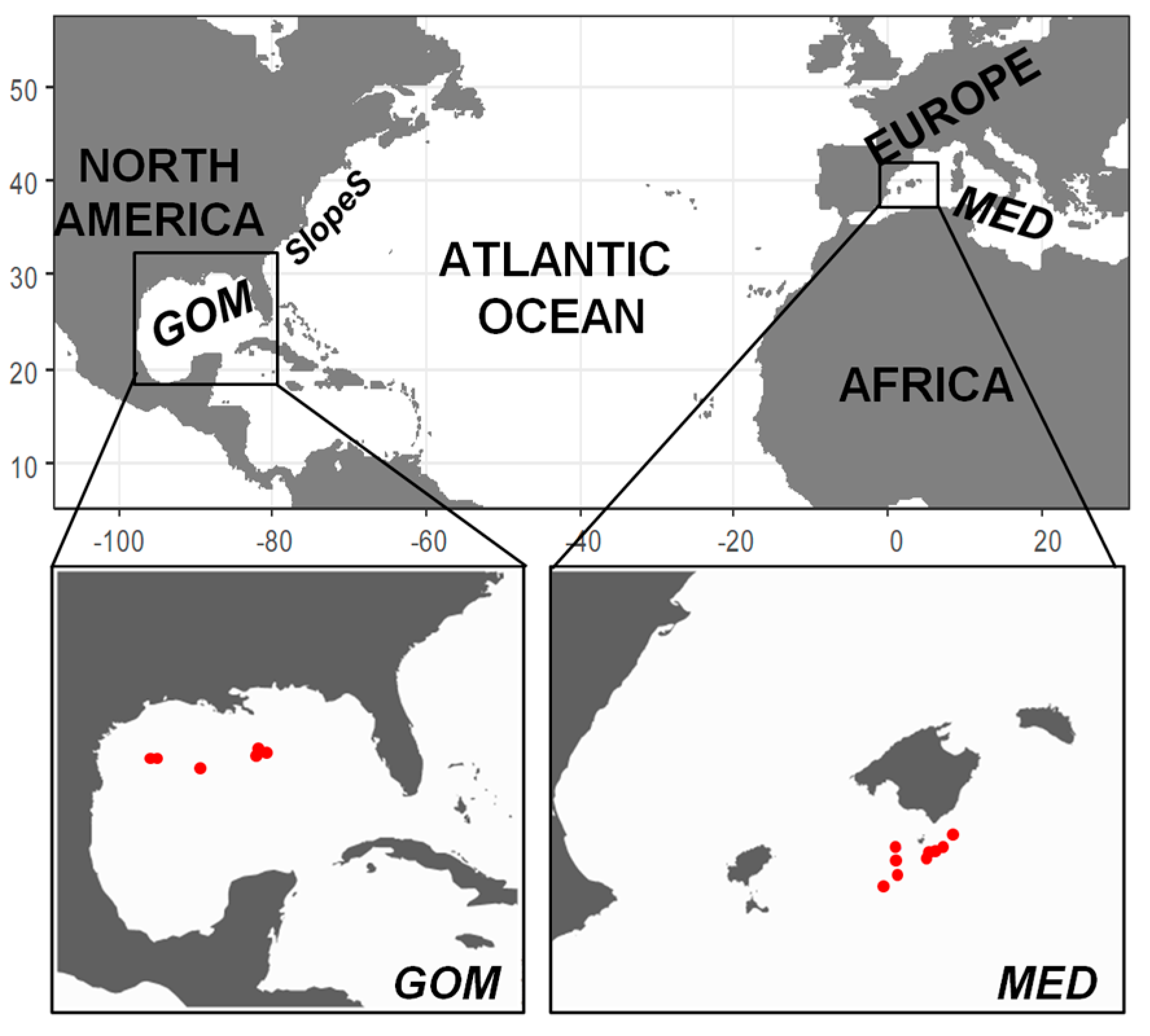
2.1. Field Sampling

Two research surveys were conducted in 2012 in the GOM and MED (Figure 1; Table S1) during the peak spawning of BFT in each area. Sampling in the GOM was conducted from April 24 to May 28 aboard the NOAA research vessel R/V Gordon Gunter, and around the Balearic Islands (MED) from July 9 to 14 on board of the R/V Ramon Margalef.

In both areas, the first part of the cruise consisted of a series of surface ichthyoplankton samplings using a ~1 mm mesh neuston net (GOM) and of oblique tows using a 90 cm diameter Bongo net equipped with 500 µm mesh (MED) over a systematic grid (see [22] for a detailed description of the systematic grid sampled in both areas). To identify stations with high density of tuna larvae, sampling devices in both surveys were deployed with flowmeters to measure the volume of filtered water by the nets. Once an acceptable number of tuna larvae was found, stratified vertical hauls were conducted at 6 stations in the GOM and 9 in the MED respectively (Table S1). Samples were collected with a 1 m² multiple opening/closing net and environmental sensing system (MOCNESS), fitted with 505 µm mesh. Samples were collected from depth ranges of 0–10 m, 10–20 m, 20–30 m, 30–40 m, and 40–50 m. In the MED, the same depth ranges were sampled (0–10 m, 10–20 m, 20–30 m, 30–40 m, and 40–50 m) and a deeper range of 50–60 m was also sampled. The GOM samples were preserved in 95% ethanol. The MED samples were preserved immediately in a solution of ~4% borax-buffered formaldehyde and seawater. At each station, a CTD was deployed to obtain vertical profiles of temperature (°C), salinity, fluorescence (mg·m⁻³) and dissolved oxygen (mL·L⁻¹). A Sea-Bird Electronics SBE 9plus CTD was used in the GOM and a Sea-Bird Electronics SBE 9 CTD in the MED.

2.2. Description of Assemblages: Taxa and Groups by Adult Habitat

In the laboratory, vertically stratified samples were sorted and identified to the lowest taxonomic level possible. In the GOM survey, the Polish Plankton Sorting and Identification Center in Szczecin, Poland processed the fish larvae. In the MED, larvae were processed at the Centro Oceanográfico de Baleares (COB) by experts in larval fish taxonomy using identification guides for the area [35,36]. The number of larvae captured in each depth range in both areas was standardized to number of larvae per 1000 m³.

The weighted mean depth (WMD) in the water column was calculated for each taxon at each area following [37]. For the common taxa in both areas, the WMDs were compared visually to search for evidence of differences in the vertical position of larvae.

For descriptive purposes and taking into account the high number of taxa found, taxa were grouped in 5 categories based on their adult habitat following [38]: bathypelagic, demersal, mesopelagic, ocean pelagic, and coastal pelagic. The percentage of total abundance of these groups was also calculated for each spawning ground.

2.3. Influence of Environment on the Vertical Distribution of the Assemblages

The influence of environmental variables on the vertical structure of the larval fish assemblage was studied using a combination of the nonmetric multi-dimensional scaling (NMDS) and generalized additive models (GAM). The combination of multi-dimensional scaling (MDS) and GAM is not new as it was applied for the first time to terrestrial ecology [39] and currently extending its applications in other environmental sciences [40]. In marine sciences, Siddon [41] was the first to apply this method to describe gradients in fish larvae species composition relative to environmental drivers in the Southeastern Bering Sea. Recent studies extended its use to other meroplankton species and megafauna [42,43]. The effectiveness of this approach depends on how likely the community structure can be summarized in several gradients regarding the physiographical, hydrographical and biological components of the seascape [42]. In such cases, this combination of methods has proven to be a powerful tool in analyzing gradients in species composition in relation to environmental gradients.

For each spawning ground, a NMDS (“vegan” library in R) was used to summarize the multispecies density data onto two major axes [44]. Prior to analysis, data were 4th-root transformed to reduce the weight of taxa with very high densities in the analyses. Bray–Curtis similarity matrices were calculated, followed by an ordination using NMDS for both stations and depth strata. The procedure was performed with 100 random starts to find the final stable solution. We then developed a GAM using each of the NMDS axes as the dependent variable to understand the influence of environmental variables on the structure identified in the community [42]. In addition, spearman rank correlations were also used to identify which species were most strongly related to the first 2 ordination axes of the NMDS. The species whose index of correlation was significant (either positive or negative correlation, p < 0.001) were most closely related to the correlation axes of the NMDS analysis and therefore were considered the most representative species of the distribution patterns [41,42].

The environmental variables considered for each area were: sea water temperature (°C), sea water salinity, sea water fluorescence (mg m⁻³) and dissolved oxygen (mL L⁻¹). Environmental data from CTD cast recorded at 1 m depth bins were transformed to one data per depth stratum by calculating the mean value of each considered variable for each of the depth strata sampled by the MOCNESS device (0–10 m, 10–20 m, 20–30 m, 30–40 m, and 40–50 m). Prior to the model selection, collinearity among environmental covariates was tested by applying a variance inflation factor (VIF). A cut-off VIF value of 3.3 was used to get the final set of covariates [45]. Next, we adopted a backwards stepwise procedure from a first initial GAM model including all the non-colinear covariates, removing 1 non-significant covariate at a time. To obtain the final model, model selection was based on the Akaike’s information criterion (AICc).

The GAM model formulation for each area was:

$$Axi{s}_{i,w}=a+{\displaystyle \sum }_j^{j=m}{s}_j(E)+\epsilon$$

where Axis represents the score of the NMDS axis i (1 or 2) at each spawning ground w. The term $a$ represents the intercept, E a vector of m environmental covariates, s the one-dimensional non-parametric smoothing functions (cubic splines with up to a maximum of 3 df) and ɛ a Gaussian error term.

Variance contribution of each covariate was explored for each final model to assess the most relevant covariate(s) to be plotted.

3. Results

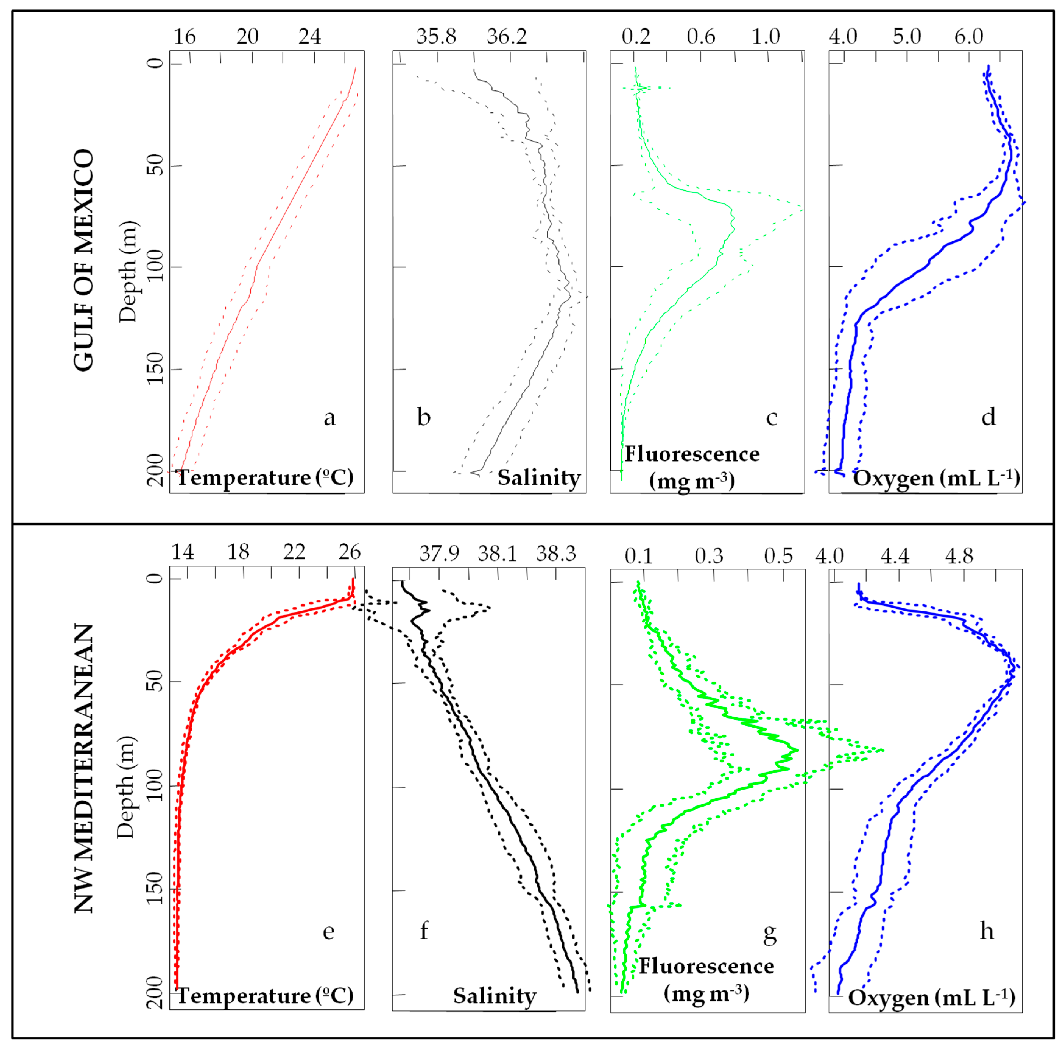
3.1. Environmental Scenario

No thermal stratification was observed in the upper 200 m of the water column in the GOM (Figure 2a–d). The vertical temperature profile was characterized by a temperature maximum of 26.4 ± 0.4 °C at the surface. Temperatures linearly decreased to 20 °C at around 95 m depth reaching a minimum temperature of 15.5 ± 0.7 °C at 200 m depth (Figure 2a). Salinity values were around 36 throughout the water column ranging from 36.07 ± 0.34 at the surface and 36.04 ± 0.11 at 200 m depth (Figure 2b). A slight maximum salinity (36.47 ± 0.05) was observed at 120 m depth. The fluorescence maximum was located around 80 m depth with a value of 1.18 ± 0.17 mg m⁻³. Surface and 200 m depth fluorescence values were 0.21 ± 0.01 mg m⁻³ and 0.13 ± 0.01 mg m⁻³ respectively (Figure 2c). Oxygen values were higher in the upper portion of the water column with values from the surface to the 50 m around 6.4 ± 0.28 mL L⁻¹ (Figure 2d). Values strongly dropped to 4.5 ± 0.45 mL L⁻¹ at 120 m depth and reached values of 4.03 ± 0.26 mL L⁻¹ at 200 m depth.

The MED was characterized by strong thermal stratification (Figure 2e–h). Temperatures ranged from maximum values of 25.5 ± 0.8 °C at the surface to a minimum value of 13.24 ± 0.02 °C at 200 m depth with a pronounced gradient at around 20 m (Figure 2e). Salinity values were lowest at the surface (37.76 ± 0.13), slightly increasing with depth (38.37 ± 0.04 at 200 m depth, Figure 2f). Fluorescence values were generally low, 0.1 ± 0.01 and 0.03 ± 0.01 mg m⁻³ at the surface and 200 m depth respectively, with maximum values of 0.86 ± 0.2 mg m⁻³ around 80 m depth (Figure 2g). Oxygen values were highest around 40 m depth, 5.57 ± 0.02 mL L⁻¹, with the lowest values measured both at the surface and at 200 m depth (4.2 ± 0.01 and 4 ± 0.21 mL L⁻¹ respectively; Figure 2h).

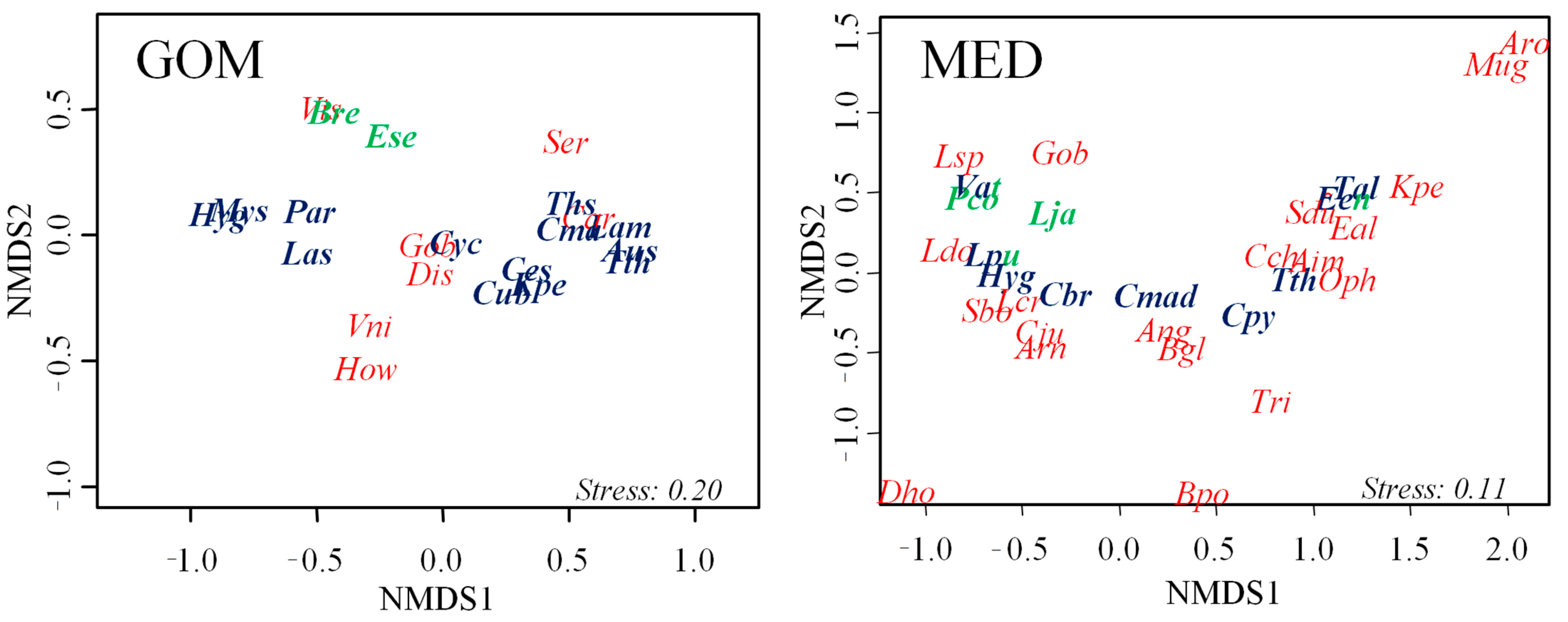
3.2. Description of Assemblages: Taxa and Groups by Adult Habitat

Using the MOCNESS, a total of 6281 fish larvae were collected and identified in the GOM and 7977 larvae in the MED. A total of 64 taxa were identified in the GOM, 19 to family level, 25 to genus, and 20 to species level. In the MED, a total of 32 taxa were identified, 5 to family level, 2 to genus and 25 to species level (

Table 1. Alphabetical list of larval fish families collected in the Gulf of Mexico (GOM) and the Mediterranean (MED); NMDS Code used to shorten taxa names in Figure 5; Habitat of the Adult (AH); Total Abundance (TA, individuals (i) 1000 m⁻³); taxon relative abundance (TA, %); Weighted Mean Depth (WMD, in m). AH Code: Bathypelagic (B); Coastal Pelagic (CP); Demersal (D); Mesopelagic (M) and Ocean Pelagic (OP).

Family	Taxa	NMDS Code	AH	GOM			MED
				TA (i × 103 m−3)	TA (%)	WMD (m)	TA (i × 103 m−3)	TA (%)	WMD (m)
Acropomatidae	Acropomatidae NI		D	20.9	0.12	38.7
Anguilliformes	Anguilliformes	Ang	D	8.5	0.05	25.6	79.1	0.03	10.95
Apogonidae	Apogon imberbis	Aim	D				42.8	0.02	15.00
Apogonidae	Apogon spp		D	20.6	0.11	5.0
Bothidae	Arnoglossus spp	Arn	D				43.3	0.02	35.00
	Bothidae NI		D	36.9	0.20	28.3
	Bothus podas	Bpo	D				43.9	0.02	15.00
	Bothus spp		D	66.2	0.36	23.1
	Engyophrys senta	Ese	D	75.7	0.42	24.7
	Trichopsetta spp		D	52.2	0.29	28.0
Bramidae	Bramidae NI		OP	17.4	0.10	18.2
Bregmacerotidae	Bregmaceros spp	Bre	CP	443.8	2.44	34.3
Carangidae	Caranx spp	Car	CP	1796.8	9.87	9.0
	Elagatis bipinnulata		CP	43.9	0.24	15.0
	Selar crumenophthalmus		CP	28.4	0.16	10.6
	Seriola durmerilii	Sdu	CP				42.8	0.02	15.00
Ceratioidei	Ceratioidei NI		B	66.3	0.36	29.5
Chlorophthalmidae	Chlorophthalmus agassizi		D	30.2	0.17	24.1
	Chlorophthalmus brasiliensis		D	21.9	0.12	18.5
Congridae	Congridae NI		D	50.3	0.28	24.6
Coryphaenidae	Coryphaena hippurus		OP	58.3	0.32	8.0
Cynoglossidae	Symphurus spp		D	41.3	0.23	24.8
Engraulidae	Engraulis encrasicolus	Een	CP				2579.7	1.04	7.05
Gempylidae	Diplospinus multistriatus		M	39.7	0.22	44.1
	Epinnula magistralis		M	26.8	0.15	24.0
	Gempylidae		M	18.0	0.10	45.0
	Gempylus serpens		M	36.0	0.20	10.2
Gobiidae	Gobiidae	Gob	D	290.2	1.59	26.6	46.5	0.02	45.00
Gonostomatidae	Cyclothone spp	Cyc	M	3266.8	17.94	18.2
	Gonostomatidae NI		M	29.5	0.16	29.4
	Cyclothone braueri	Cbr	M				77407.8	31.08	25.31
	Cyclothone pygmaea	Cpy	M				4560.6	1.83	12.75
	Lestidiops jayakari	Lja	B				778.2	0.31	41.80
	Lestidiops sphyrenoides	Lsp	B				121.9	0.05	48.28
Howellidae	Howella spp	How	B	100.6	0.55	27.7
Labridae	Coris julis	Cju	D				397.2	0.16	28.99
Lutjanidae	Pristipomoides aquilonaris		D	58.2	0.32	15.3
Mugilidae	Mugilidae NI	Mug	D				45.1	0.02	5.00
Myctophidae	Benthosema glaciale	Bgl	M				142.4	0.06	41.79
	Benthosema spp		M	31.4	0.17	26.1
	Ceratoscopelus maderensis	Cma	M	558.4	3.07	13.5	24786.9	9.95	17.84
	Ceratoscopelus spp	Ces	M	823.7	4.52	23.0
	Diaphus holti	Dho	M				42.7	0.02	25.00
	Diaphus spp	Dis	M	4671.0	25.65	21.6
	Diogenichthys atlanticus		M	32.5	0.18	40.2
	Hygophum spp	Hyg	M	196.1	1.08	41.7	68444.3	27.48	34.17
	Lampadena spp	Lam	M	335.3	1.84	9.0
	Lampanyctus crocodilus	Lcr	M				1474.5	0.59	35.67
	Lampanyctus pusillus	Lpu	M				5026.7	2.02	32.94
	Lampanyctus spp	Las	M	313.2	1.72	34.7
	Lobianchia dofleini	Ldo	M				204.7	0.08	46.68
	Myctophidae NI		M	64.4	0.35	35.4
	Myctophum punctatum		M				39.6	0.02	55.00
	Myctophum spp	Mys	M	303.9	1.67	39.9
	Notolychnus valdiviae		M	22.0	0.12	32.9
	Symbolophorus veranyi		M				40.6	0.02	55.00
Nettastomatidae	Nettastomatidae NI		B	26.1	0.14	33.1
Nomeidae	Psenes spp		OP	19.9	0.11	32.0
Ophichthidae	Ophichthidae		D	22.9	0.13	25.0
Ophichthidae	Ophichthus gomesi		D	20.4	0.11	12.2
Ophididae	Ophididae	Oph	D				42.8	0.02	15.00
Paralepididae	Paralepididae NI	Par	M	498.0	2.73	30.8
	Paralepis coregonoides	Pco	M				1086.7	0.44	38.78
	Sudis spp		M	21.1	0.12	40.2
Paralichthyidae	Cubiceps spp	Cub	D	800.6	4.40	12.5
	Etropus spp		D	25.0	0.14	18.5
	Syacium papillosum		D	69.1	0.38	25.0
Phosichthyidae	Vinciguerria attenuata	Vat	M	2.9	0.02	45.0	2604.6	1.05	43.81
	Vinciguerria nimbaria	Vni	M	259.3	1.42	28.8
	Vinciguerria spp	Vis	M	97.3	0.53	32.3
Pomacentridae	Chromis chromis	Cch	D				99.2	0.04	12.67
Scombridae	Auxis rochei	Aro	OP				45.1	0.02	5.00
	Auxis spp	Aus	OP	74.7	0.41	17.1
	Euthynnus alletteratus	Eal	OP	10.5	0.06	20.5	103.7	0.04	5.00
	Katsuwonus pelamis	Kpe	OP	343.8	1.89	19.6	32.1	0.01	5.00
	Thunnus alalunga	Tal	OP				354.8	0.14	9.56
	Thunnus spp	Ths	OP	411.7	2.26	12.3
	Thunnus thynnus	Tth	OP	417.5	2.29	7.2	58052.2	23.31	8.07
Scorpaenidae	Scorpaenidae NI		D	20.0	0.11	26.5
Serranidae	Anthias spp		D	30.5	0.17	17.9
	Epinephelinae NI		D	62.1	0.34	16.1
	Hemanthias spp		D	58.0	0.32	20.8
	Serranus spp	Ser	D	145.4	0.80	16.6
Stomiatidae	Stomias boa	Sbo	M				200.8	0.08	33.31
Stomiidae	Melanostomiinae NI		M	53.1	0.29	21.5
Synodontidae	Synodontidae		D	20.7	0.11	13.0
Tetraodontidae	Tetraodontidae		D	24.2	0.13	26.1
Triglidae	Triglidae	Tri	D	18.0	0.10	20.9	44.7	0.02	5.00

).

Tuna species in the Scombridae family were the main taxa contributing to the ocean pelagic category in both areas, although in the GOM Coryphaena spp. and Psenes spp. were also captured (Table 1). The abundance of BFT in the MED was one order of magnitude higher than in the GOM and two orders of magnitude higher than the abundance of any other scombrid within the MED assemblage. In the GOM, the abundances of Thunnus spp. and Katsowonus pelamis were similar and one order of magnitude higher than any other ocean pelagic taxa in the area. The contribution of the ocean pelagic taxa to the total larval fish abundance was relatively low in the GOM, 7.7% of the total abundance of larvae, whereas in the MED the ocean pelagic group was the second most important group, after the mesopelagic group, representing around 23.5% of the total abundance. The mesopelagic group dominated the assemblages in both areas accounting for 64.5% and 74.7% of the total larval fish abundance for the GOM and the MED, respectively. The number of mesopelagic taxa was higher in the GOM (23 taxa) than in the MED (14 taxa, Table 1). The most abundant taxa in both areas belonged to the Myctophidae and Gonostomatidae families. Taxa from the genus Diaphus, Ceratoscopelus, Lampadena, and Lampanyctus were the most abundant Myctophidae in the GOM and Hygophum, Ceratoscopelus, and Lampanyctus genus were the most abundant Myctophids in the MED. The genus Cyclothone was the primary taxa of Gnosmostomatidae in both areas.

In the GOM, the taxa belonging to the demersal and coastal pelagic groups contributed similarly to the total abundance of larvae (13.1% and 12.9%, respectively), whereas there was almost no contribution of the bathypelagic taxa to the overall larval fish abundance (1.1%). In contrast, in combination, the coastal pelagic, demersal and bathypelagic groups represented less than 2% of the total larval abundance in the MED.

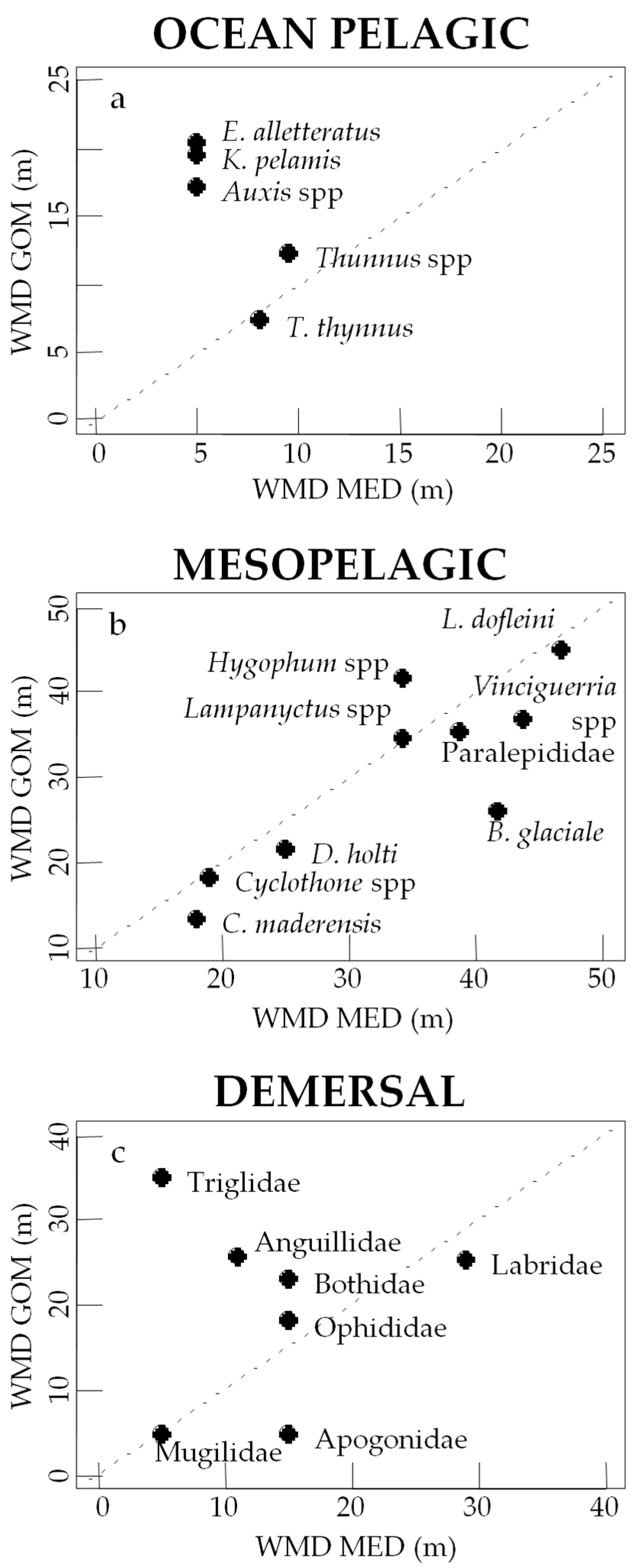
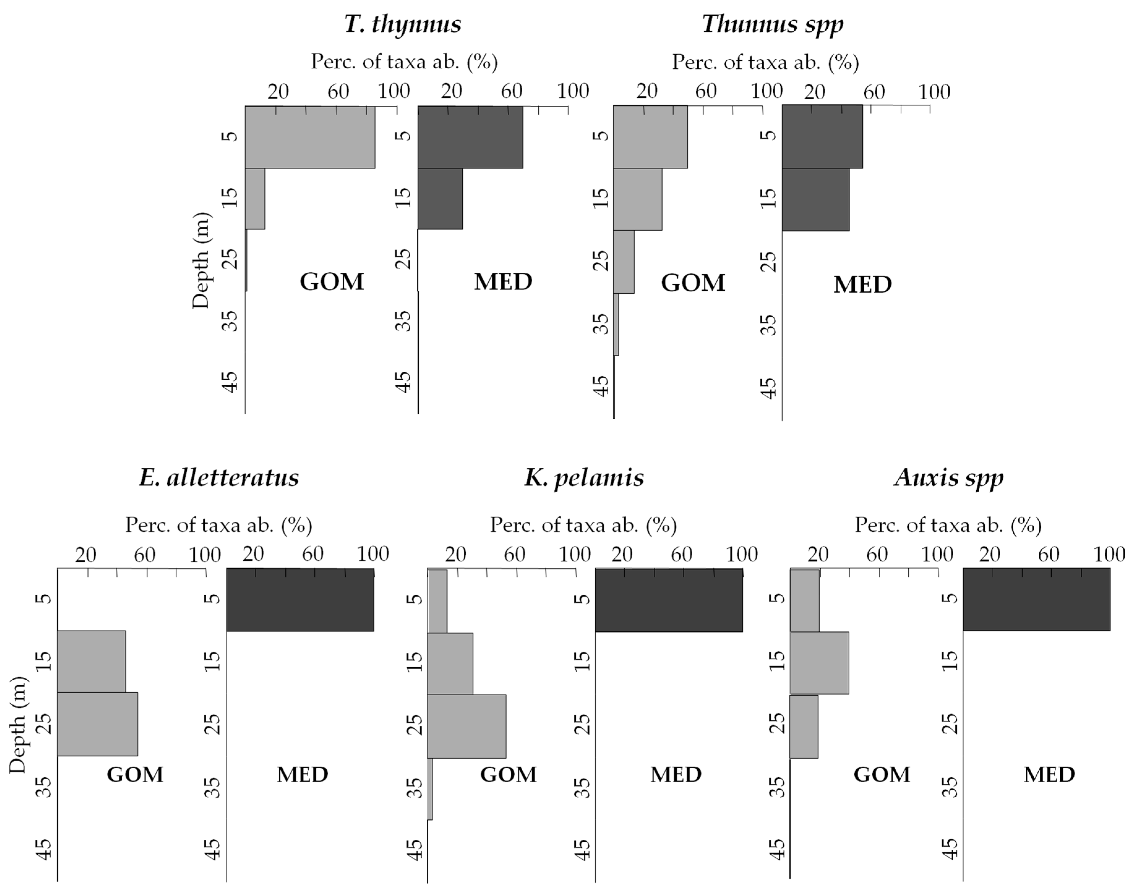
3.3. Vertical Distribution of Assemblages

Most scombrids were deeper in the GOM than the MED. The genus Thunnus were observed at similar depth ranges between 7 and 12 m in both areas (Figure 3a, Table 1) and the vertical distribution of BFT was very similar in both areas (Figure 3a). This species was distributed from the surface to 30 m depth, with most of the individuals found in the top 10 m (Figure 4). Individuals from the genus Thunnus spp. were found at all depths in the GOM (Figure 4), although most larvae were found at depths ranging from 0 to 20 m, which is the same range where all the Thunnus alalunga in the MED were found (Figure 4). In the MED, the rest of the scombrids were found in the upper 10 m of the water column, whereas in the GOM abundances peaked at 15–25 m, depending on the species (Figure 3a and Figure 4).

Most of the common mesopelagic taxa occupied similar depth ranges in the GOM and the MED except for Hygophum spp. (deeper in GOM) and Benthosema glaciale (deeper in MED, Figure 3b). Finally, the depth distribution of three families in the demersal group (Triglidae, Anguillidae and Apogonidae) differed between the GOM and MED (Figure 3c). Given that coastal pelagic and bathypelagic families from the GOM and the MED did not overlap, comparison of the vertical distribution between regions was not possible.

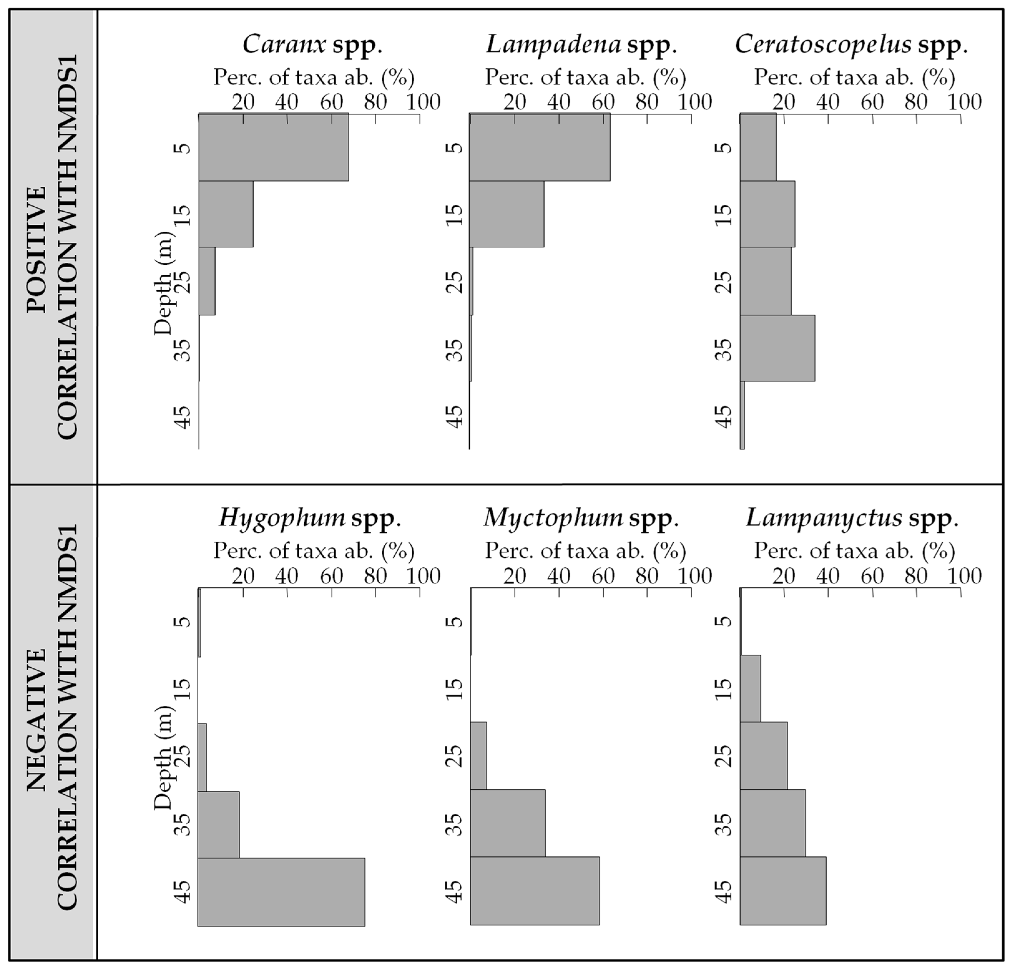
3.4. Influence of Environment on the Vertical Distribution of the Assemblages

The NMDS allowed us, at each area separately, to summarize the multi-taxa density data onto two major axes with acceptable stress values (0.20 for the GOM and 0.11 for the MED, Figure 5). Spearman rank correlations among taxa and the first NMDS axes for each area were calculated (Figure 5). The best-fit GAM models for the first axis (Axis 1) of the GOM and MED NMDSs explained, respectively, 44 and 66.9% of the variance (

Table 2. Best-fit general additive models (GAMs) obtained for each nonmetric multi-dimensional scaling (NMDS) axis (in italics) and results of each GAM model test for the Gulf of Mexico. a = intercept, s = smoothing functions, ε = error term. Std. Error: Standard error; edf: degrees of freedom; Ref.df: reference degrees of freedom used in computing test statistic and the p-values F: F-test values. Covariates for the models are plotted in Figure S1. Signif. codes: 0 “***” 0.001 “**” 0.01 “*” 0.05 “.” 0.1 “ ” 1.

Axis 1 $$GOM\_Axi{s}_1=a+s_{1 }\left(Salinity\right)+s_{2 }\left(Fluorescence\right)+\epsilon$$
Parametric coefficients	Estimate	Std. Error
a (Intercept)	0.003	0.029
Smooth terms	edf	Ref.df	F	p-value
s1 (Salinity)	1.875	1.984	10.54	5.97 × 10−5 ***
s2 (Fluorescence)	1.883	1.986	19.56	8.39 × 10−8 ***
	R-sq.(adj) = 0.418		Deviance explained = 44%
Axis 2 $$GOM\_Axi{s}_2=a+s_{1 }\left(Salinity\right)+s_{2 }\left(Fluorescence\right)+\epsilon$$
Parametric coefficients	Estimate	Std. Error
a (Intercept)	0.012	0.034
Smooth terms	edf	Ref.df	F	p-value
s1 (Salinity)	1.884	1.986	4.1	0.027 *
s2 (Fluorescence)	1	1	4.90	0.029 *
	R-sq.(adj) = 0.07		Deviance explained = 9.66%

and

Table 3. Best-fit general additive models (GAMs) obtained for the first nonmetric multi-dimensional scaling (NMDS) axis (in italics) and results of each GAM model test for the Mediterranean. a = intercept, s = smoothing functions, ε = error term. Std. Error: Standard error; edf: degrees of freedom; Ref.df: reference degrees of freedom used in computing test statistic and the p-values F: F-test values. Covariate for the model is plotted in Figure S2. Signif. codes: 0 “***” 0.001 “**” 0.01 “*” 0.05 “.” 0.1 “ ” 1.

Axis 1 $$MED\_Axi{s}_1=a+s_{1 }\left(Temperature\right)+\epsilon$$
Parametric coefficients	Estimate	Std. Error
a (Intercept)	−2.5 × 10−11	0.06
Smooth terms	edf	Ref.df	F	p-value
s1 (Temperature)	1	1	76.75	<2 × 10−12 ***
	R-sq.(adj) = 0.66		Deviance explained = 69.2%

). The best-fit model for the second axis (Axis 2) in GOM explained 9.66% of the variance and no best-fit model was found for the MED Axis 2.

In the GOM, the covariates that explained Axis 1 of the vertical distribution of the species were a combination of water salinity and fluorescence (Table 2, Figure S1). Specifically, we found negative relationships with both.

The taxa significantly correlated with Axis 1 in the GOM were meso- and ocean pelagic species except for the coastal Caranx spp. (all tests p < 0.01, Figure 5). Most individuals from the ocean pelagic group were positively correlated with Axis 1 (e.g., Katsuwonus pelamis, T. thynnus, Coryphaena hippurus) whereas taxa from the mesopelagic group were both positively and negatively correlated with Axis 1 (e.g., Lampadena spp., Ceratoscopelus spp., Lampanyctus spp.). Most taxa positively correlated with Axis 1 were found in the upper portion of the water column (Figure 4 and Figure 6), except for Ceratoscopelus spp., which was present in all the depth strata. Conversely, taxa negatively correlated with Axis 1 showed deeper vertical distributions (Figure 6).

In the MED, the covariate in the GAM that best explained Axis 1 was temperature. An optimum was observed in the partial effect of temperature on the vertical distribution of larvae at ~25.5 °C (Figure S2). No significant covariates were found for the GAM of the Axis 2.

Taxa from the meso- and ocean pelagic groups were correlated with Axis 1 (all tests p < 0.01, Figure 1). Ocean pelagic taxa (BFT and T. alalunga) were positively correlated with Axis 1, whereas mesopelagics were both positively and negatively correlated. As in the GOM, taxa positively correlated with the Axis 1 in the MED were distributed more towards the surface (Figure 4 and Figure 7) and those negatively correlated were more deeply distributed (Figure 7).

In the GOM, Axis 2 was explained by a negative linear relationship with fluorescence and a range (~36.1–36.45) of salinity values (Table 2, Figure S2). The taxa significantly correlated with this axis were members of the coastal pelagic, demersal and bathypelagic groups (p < 0.01; e.g., Bregmaceros spp., Serranus spp., Nettastomatidae). In the MED, taxa correlated with the Axis 2 were a mix of mesopelagic, bathypelagic and coastal pelagic (e.g., Vinciguerria attenuata, Lestidiops jayakari, Engraulis encrasicolus).

4. Discussion

This study finds that temperature influences vertical distribution of larvae in the MED and a combination of salinity and fluorescence values in the GOM. Our findings support previous work that has demonstrated that temperature is the primary variable explaining vertical distribution of fish larvae in regions where the water column is characterized by a strong thermocline [5,26,46]. The strong thermal gradient in the MED also drives the composition of the larval fish assemblage where there is a clear faunal shift from above to below the thermocline (0–25 m). Our results are unique in that they show tuna larvae also inhabit the upper water layers in the GOM, where there is no thermal stratification and where the temperatures greater than 20 °C persist to depths of 80–100 m. The vertical distribution of the larval fish assemblage in the GOM is correlated with a combination of environmental variables including salinity and fluorescence values characteristic of surface waters.

The composition of the larval fish assemblage associated with BFT larvae in both spawning areas is strikingly similar, despite evidence that different environmental drivers influence the vertical structure of the assemblages. BFT larvae co-occur in the upper water layer with other tuna and specific mesopelagic species in both ecosystems. Co-occurrence of multiples species of tuna larvae in the first upper 20 m of the water column has been reported throughout the world [16,17,21,26,47,48,49,50]. Our results corroborate these findings. In the MED, all tuna inhabited the upper 20 m, whereas in the GOM, tuna were found down to depths of 30 m, though most (66%) were in the upper 20 m. The WMD of Thunnus larvae was almost same between GOM and MED however the WMD of the other scomber larvae in the MED was clearly shallower than that in the GOM (Figure 3a and Figure 4). In the MED, the thermocline is a sharp temperature boundary layer for the scombrid larvae, and they are forced to coexist in the first 20 m, whereas the optimal temperatures for scombrid larvae can be found from surface down to 100 m depth in the GOM. Under those conditions, scomber larvae can avoid coexistence among them by selecting a wider range of depths. Anyway, in the GOM, their condition of visual predators might also limit their vertical expansion. Horizontal habitat segregation in scombrid larvae has already been documented in the Pacific [8], in the GOM [23] and in the MED [51]. It is to be expected that the same segregation can occur in the vertical distribution of taxa if the environmental conditions are within the taxa specific limits.

We found striking similarities in the depth distribution of the mesopelagic group between the two study areas. We hypothesize that the depth distribution of these individuals is influenced by the availability of their prey [52]. In the GOM, more than half of the zooplankton biomass is found in the upper 200 m, with the majority of that occurring in the upper 50 m [53]. In the MED, during the stratified period (when tuna spawning season takes place), zooplankton exhibits a very structured vertical pattern, with some groups presenting daily vertical migrations (copepods and ostracoda), whereas others remain both night and day at upper (cladocera) or deeper (appendicularia) layers [54].

In contrast with the mesopelagic group, the demersal group exhibited quite different vertical distributions in the GOM and MED. Since the dispersal phase of a demersal fish must result in the fish returning to the benthic adult habitat, the dispersal trajectory of the larvae must be more precise than for pelagic individuals [55]. As vertical distribution strongly influences horizontal advection, it is not surprising that the vertical distribution of these species differs between regions, as the oceanographic processes influencing circulation differ. In the MED, only the Labridae family was found deeper than the thermocline barrier (~20m) whereas families that show the ability to choose deeper distributions in the GOM (Triglidae and Anguillidae) remain in shallow waters in the MED. Apart from the abiotic variables included in the analysis, competition and other ecological interactions might be the cause of differences in the assemblage’s vertical distribution. In the MED, the shallow strong thermocline acts as a boundary layer for most of the taxa vertical distributions. The different groups must combine their physiological requirements in terms of abiotic tolerance, with the food availability and with the ecological interactions with other taxa such as competition or predation in a very narrow vertical layer. The absence of that shallow boundary layer in the GOM allows the assemblage to be more expanded in the vertical. In a transect crossing the tropical to equatorial Atlantic Ocean, with strong thermal stratification down to ~100 m, larval fish assemblages were found also occupying different vertical positions in relation to the physiological and ecological constraints [5]. The relative distribution in the vertical among taxa was very similar to the one found in the GOM.

Diel changes in the vertical position of fish larvae have not been addressed in this work. Sampling in GOM and in the MED was equally distributed throughout the 24 h of the day (Table S1). No day-night differences were found among catches at the different depth strata. Previous studies in the GOM found no day-night differences in vertical positions or abundances of tuna larvae [56]. In the MED, winter and summer diel vertical distributions of fish larvae from the surface to 200 m depth were systematically studied during intensive 48 h sampling periods [54]. Most of the taxa that were found during summer at depth > 50 m did not show differences greater than 10 m in their day or night vertical positions. In the Atlantic Ocean, no day-night differences were found in the vertical pattern of most fish larvae [5]. However, transforming stages of some mesopelagic taxa exhibited diel vertical migration. Very few transforming-stage individuals were found in our catches and they were not included in the analyses. Due to the narrow vertical range inhabited by tuna larvae, the study of ontogenetic diel migrations would require sampling with greater vertical resolution (<10 m) tows.

Water temperatures above 20 °C are related to suitable larval habitats for tuna species [18,19]. In scenarios characterized by having a strong thermocline, this minimum temperature limit for the larval distribution (20 °C) has been linked to the vertical distribution of tuna larvae above the thermocline (e.g., [26,46]), but it does not explain the vertical distribution of the tuna larvae found in the GOM, where the 20 °C limit is found to 95m deep and most of tuna larvae (80.6%) inhabit the upper 30 m.

Behavioral rearing experiments simulating vertical temperature gradients have demonstrated that BFT and bonito larvae are distributed throughout the water column in isothermal conditions as opposed to occupying specific depths when there is a sharp temperature gradient [25]. In our study, regardless of thermal conditions, tuna larvae were primarily found in surface waters, suggesting another abiotic or biotic factor influences their vertical distribution. We hypothesize light level is the additional variable that influences the vertical distribution of tuna larvae. Along with temperature, light is among the most common of vertical cues for larvae in the ocean [57]. BFT larvae are visual predators, feeding mainly during daylight hours [58]. We propose that the vertical habitat of BFT larvae is defined by water masses with a combination of suitable temperature, high forage biomass, clear water and sufficient light level to observe prey [59]. Unfortunately, no reliable light or turbidity data were available for the present work, but the coexistence with other ichthyoplankton groups in the first meters of the water column, where incident light is maximum, is compatible with the idea of where a visual predator should be positioned in the vertical to maximize foraging possibilities.

In recent years, the annual densities of BFT larvae have been increasing in both the MED and GOM [33,34]. MED densities are significantly higher than those reported in the GOM. Knowledge of which species comprise the larval fish assemblages in major tuna spawning grounds is key to understand the ecological role of tuna larvae within the community. For BFT larvae, finding larval prey at the right place in the right time improves larval growth and survival [19]. Rearing experiments have demonstrated selective piscivory in tuna larvae [60]; however, we still know very little about the prey ingested by tuna in the wild. The narrow available vertical habitat for all the larval fish assemblage in the MED might force the coexistence of tuna larvae with its potential prey, unless horizontal niche segregation is possible. That could be one of the reasons behind the high tuna fish larvae densities found in the MED. Using common methodology is crucial when comparing larval fish assemblages between regions. The use of similar nets, sampling methodologies and environmental variables can help to compare spawning areas while avoiding significant methodological issues [56,61]. Studies such as this one improve our knowledge about the composition of the larval fish community and expand our knowledge of the detailed vertical distribution of prey and tuna in their spawning grounds. One example is the high abundances of specific species of mesopelagic larvae found together with tuna that may ensure the availability of prey for the tuna larvae.

5. Conclusions

Our results emphasize that tuna larvae occupy the upper portion of the water column regardless of whether the water column is stratified. Furthermore, we find that regardless of spawning ground, multiple species of tuna coexist. Finally, there are striking similarities in the species compositions between the two areas despite the thermal and regional differences. In the future, we propose that models of prey encounter be developed to disentangle the effects of light and temperature on the vertical distribution of the larva. Work such as this is only possible with standardized methodologies, and comparative studies such as this one provide important insights on the larval ecology of tuna and associated species. Furthermore, they allow researchers to understand which trends they observe are local subpopulation dynamics and which are population level responses, a key to effective fisheries management.

References

1. Loreau, M. Linking biodiversity and ecosystems: Towards a unifying ecological theory. Philos. Trans. R. Soc. B Biol. Sci. 2010, 365, 49–60. [Google Scholar] [CrossRef] [PubMed] [Green Version]
2. Maureaud, A.; Andersen, K.H.; Zhang, L.; Lindegren, M. Trait-based food web model reveals the underlying mechanisms of biodiversity-ecosystem functioning relationships. J. Anim. Ecol. 2020, 89, 1497–1510. [Google Scholar] [CrossRef] [PubMed]
3. Hsieh, C.H.; Kim, H.J.; Watson, W.; Di Lorenzo, E.; Sugihara, G. Climate-driven changes in abundance and distribution of larvae of oceanic fishes in the southern California region. Glob. Chang. Biol. 2009, 15, 2137–2152. [Google Scholar] [CrossRef]
4. Leis, J.M. Are Larvae of Demersal Fishes Plankton or Nekton? Adv. Mar. Biol. 2006, 51, 58–141. [Google Scholar]
5. Olivar, M.P.; Contreras, T.; Hulley, P.A.; Emelianov, M.; López-Pérez, C.; Tuset, V.; Castellón, A. Variation in the diel vertical distributions of larvae and transforming stages of oceanic fishes across the tropical and equatorial Atlantic. Prog. Oceanogr. 2018. [Google Scholar] [CrossRef]
6. Reygondeau, G.; Maury, O.; Beaugrand, G.; Fromentin, J.M.; Fonteneau, A.; Cury, P. Biogeography of tuna and billfish communities. J. Biogeogr. 2012, 39, 114–129. [Google Scholar] [CrossRef] [Green Version]
7. Olson, R.J.; Young, J.W.; Ménard, F.; Potier, M.; Allain, V.; Goñi, N.; Logan, J.M.; Galván-Magaña, F. Bioenergetics, Trophic Ecology, and Niche Separation of Tunas. Adv. Mar. Biol. 2016, 74, 199–344. [Google Scholar] [CrossRef] [PubMed]
8. Tawa, A.; Kodama, T.; Sakuma, K.; Ishihara, T.; Ohshimo, S. Fine-scale horizontal distributions of multiple species of larval tuna off the Nansei Islands, Japan. Mar. Ecol. Prog. Ser. 2020, 636, 123–137. [Google Scholar] [CrossRef]
9. Llopiz, J.K.; Hobday, A.J. A global comparative analysis of the feeding dynamics and environmental conditions of larval tunas, mackerels, and billfishes. Deep Res. Part II Top. Stud. Oceanogr. 2015, 113, 113–124. [Google Scholar] [CrossRef]
10. Richardson, D.E.; Marancik, K.E.; Guyon, J.R.; Lutcavage, M.E.; Galuardi, B.; Lam, C.H.; Walsh, H.J.; Wildes, S.; Yates, D.A.; Hare, J.A. Discovery of a spawning ground reveals diverse migration strategies in Atlantic bluefin tuna (Thunnus thynnus). Proc. Natl. Acad. Sci. USA 2016, 113, 3299–3304. [Google Scholar] [CrossRef] [Green Version]
11. McGowan, M.F.; Richards, W.J. Bluefin tuna, Thunnus thynnus, larvae in the Gulf Stream off the southeastern United States: Satellite and shipboard observations of their environment. Fish. Bull. 1989, 87, 615–631. [Google Scholar]
12. Cowen, R.K.; Paris, C.B.; Srinivasan, A. Scaling of Connectivity in Marine Populations. Science 2006, 311, 522–527. [Google Scholar] [CrossRef] [PubMed] [Green Version]
13. Hernandez, F.J.; Hare, J.A.; Fey, D.P. Evaluating diel, ontogenetic and environmental effects on larval fish vertical distribution using generalized additive models for location, scale and shape. Fish. Oceanogr. 2009. [Google Scholar] [CrossRef]
14. Richardson, D.E.; Llopiz, J.K.; Guigand, C.M.; Cowen, R.K. Larval assemblages of large and medium-sized pelagic species in the Straits of Florida. Prog. Oceanogr. 2010, 86, 8–20. [Google Scholar] [CrossRef] [Green Version]
15. Rooker, J.R.; Simms, J.R.; David Wells, R.J.; Holt, S.A.; Holt, G.J.; Graves, J.E.; Furey, N.B. Distribution and habitat associations of billfish and swordfish larvae across mesoscale features in the gulf of Mexico. PLoS ONE 2012, 7. [Google Scholar] [CrossRef] [PubMed] [Green Version]
16. Davis, T.L.O.; Jenkins, G.P.; Young, J.W. Patterns of horizontal distribution of the larvae of southern bluefin (Thunnus maccoyii) and other tuna in the Indian Ocean. J. Plankton Res. 1990, 12, 1295–1314. [Google Scholar] [CrossRef]
17. Boehlert, G.W.; Mundy, B.C. Vertical and onshore-offshore distributional patterns of tuna larvae in relation to physical habitat features. Mar. Ecol. Prog. Ser. 1994, 107, 1–14. [Google Scholar] [CrossRef]
18. Schaefer, K.M. Assessment of skipjack tuna (Katsuwonus pelamis) spawning activity in the eastern Pacific Ocean. Fish. Bull. 2001, 99, 343–350. [Google Scholar]
19. Reglero, P.; Tittensor, D.P.D.; Álvarez-Berastegui, D.; Aparicio-González, A.; Worm, B. Worldwide distributions of tuna larvae: Revisiting hypotheses on environmental requirements for spawning habitats. Mar. Ecol. Prog. Ser. 2014, 501, 207–224. [Google Scholar] [CrossRef] [Green Version]
20. Muhling, B.A.; Lamkin, J.T.; Alemany, F.; García, A.; Farley, J.; Ingram, G.W.; Berastegui, D.A.; Reglero, P.; Carrion, R.L. Reproduction and Larval Biology in Tunas, and the Importance of Restricted Area Spawning Grounds. Rev. Fish Biol. Fish. 2017, 27. [Google Scholar] [CrossRef]
21. Torres, A.P.; Reglero, P.; Balbin, R.; Urtizberea, A.; Alemany, F. Coexistence of larvae of tuna species and other fish in the surface mixed layer in the NW Mediterranean. J. Plankton Res. 2011. [Google Scholar] [CrossRef]
22. Muhling, B.A.; Reglero, P.; Ciannelli, L.; Alvarez-Berastegui, D.; Alemany, F.; Lamkin, J.T.; Roffer, M.A. Comparison between environmental characteristics of larval bluefin tuna Thunnus thynnus habitat in the Gulf of Mexico and western Mediterranean Sea. Mar. Ecol. Prog. Ser. 2013, 486, 257–276. [Google Scholar] [CrossRef] [Green Version]
23. Pruzinsky, N.M.; Milligan, R.J.; Sutton, T.T. Pelagic Habitat Partitioning of Late-Larval and Juvenile Tunas in the Oceanic Gulf of Mexico. Front. Mar. Sci. 2020, 7, 1–13. [Google Scholar] [CrossRef]
24. Margulies, D.; Suter, J.M.; Hunt, S.L.; Olson, R.J.; Scholey, V.P.; Wexler, J.B.; Nakazawa, A. Spawning and early development of captive yellowfin tuna (Thunnus albacares). Fish. Bull. 2007, 105, 249–265. [Google Scholar]
25. Reglero, P.; Ortega, A.; Balbín, R.; Abascal, F.J.; Medina, A.; Blanco, E.; de la Gándara, F.; Alvarez-Berastegui, D.; Hidalgo, M.; Rasmuson, L.; et al. Atlantic bluefin tuna spawn at suboptimal temperatures for their offspring. Proc. R. Soc. B Biol. Sci. 2018. [Google Scholar] [CrossRef]
26. Satoh, K. Horizontal and vertical distribution of larvae of Pacific bluefin tuna Thunnus orientalis in patches entrained in mesoscale eddies. Mar. Ecol. Prog. Ser. 2010, 404, 227–240. [Google Scholar] [CrossRef]
27. Reglero, P.; Blanco, E.; Alemany, F.; Ferrá, C.; Alvarez-Berastegui, D.; Ortega, A.; De La Gándara, F.; Aparicio-González, A.; Folkvord, A. Vertical distribution of Atlantic bluefin tuna Thunnus thynnus and bonito Sarda sarda larvae is related to temperature preference. Mar. Ecol. Prog. Ser. 2018, 594, 231–243. [Google Scholar] [CrossRef] [Green Version]
28. Kodama, T.; Ohshimo, S.; Tawa, A.; Furukawa, S.; Nohara, K.; Takeshima, H.; Chiba, S.N.; Ishihara, T.; Sawai, E.; Kawazu, M.; et al. Vertical distribution of larval Pacific bluefin tuna, Thunnus orientalis, in the Japan Sea. Deep Res. Part II Top. Stud. Oceanogr. 2020, 175. [Google Scholar] [CrossRef]
29. Álvarez, I.; Rodríguez, J.M.; Catalán, I.A.; Hidalgo, M.; Álvarez-Berastegui, D.; Balbín, R.; Aparicio-González, A.; Alemany, F. Larval fish assemblage structure in the surface layer of the northwestern Mediterranean under contrasting oceanographic scenarios. J. Plankton Res. 2015, 37. [Google Scholar] [CrossRef] [Green Version]
30. Rodriguez, J.M.M.; Alvarez, I.; Lopez-Jurado, J.L.L.; Garcia, A.; Balbin, R.; Alvarez-Berastegui, D.; Torres, A.P.P.; Alemany, F. Environmental forcing and the larval fish community associated to the Atlantic bluefin tuna spawning habitat of the Balearic region (Western Mediterranean), in early summer 2005. Deep Res. Part I Oceanogr. Res. Pap. 2013, 77, 11–22. [Google Scholar] [CrossRef] [Green Version]
31. Alemany, F.; Quintanilla, L.; Velez-Belchí, P.; García, A.; Cortés, D.; Rodríguez, J.M.; Fernández de Puelles, M.L.; González-Pola, C.; López-Jurado, J.L. Characterization of the spawning habitat of Atlantic bluefin tuna and related species in the Balearic Sea (western Mediterranean). Prog. Oceanogr. 2010, 86, 21–38. [Google Scholar] [CrossRef]
32. Alemany, F.; Deudero, S.; Morales-Nin, B.; López-Jurado, J.L.; Jansà, J.; Palmer, M.; Palomera, I. Influence of physical environmental factors on the composition and horizontal distribution of summer larval fish assemblages off Mallorca island (Balearic archipelago, western Mediterranean). J. Plankton Res. 2006, 28, 473–487. [Google Scholar] [CrossRef] [Green Version]
33. Muhling, B.A.; Lamkin, J.T.; Richards, W.J. Decadal-scale responses of larval fish assemblages to multiple ecosystem processes in the northern Gulf of Mexico. Mar. Ecol. Prog. Ser. 2012, 450, 37–53. [Google Scholar] [CrossRef] [Green Version]
34. Ingram, G.W.; Alvarez-Berastegui, D.; Reglero, P.; Balbín, R.; García, A.; Alemany, F. Incorporation of habitat information in the development of indices of larval bluefin tuna (Thunnus thynnus) in the Western Mediterranean Sea (2001–2005 and 2012–2013). Deep Res. Part II Top. Stud. Oceanogr. 2017. [Google Scholar] [CrossRef]
35. Alemany, F. Ictioplancton del Mar Balear; Universitat de les Illes Balears: Palma, Spain, 1997. [Google Scholar]
36. Rodríguez, J.M.; Alemany, F.; García, A. A Guide to the Eggs and Larvae of 100 Common Western Mediterranean Sea Bony Fish Species; FAO: Rome, Italy, 2017. [Google Scholar]
37. Fortier, L.; Leggett, W.C. Vertical migrations and transport of larval fish in a partially mixed estuary. Can. J. Fish. Aquat. Sci. 1983, 40, 1543–1555. [Google Scholar] [CrossRef]
38. Durazo-Arvizu, R.; Gaxiola-Castro, G. Dinámica Del Ecosistema Pelágico Frente a Baja California 1997–2007. In Diez Años de Investigaciones Mexicanas de La Corriente de California; Durazo-Arvizu, R., Gaxiola-Castro, G., Eds.; NE/CICESE/UABC/SEMARNAT: Ensenada, Mexico, 2010. [Google Scholar]
39. Goring, S.; Pellatt, M.G.; Lacourse, T.; Walker, I.R.; Mathewes, R.W. A new methodology for reconstructing climate and vegetation from modern pollen assemblages: An example from British Columbia. J. Biogeogr. 2009, 36, 626–638. [Google Scholar] [CrossRef]
40. Muenchow, J.; Feilhauer, H.; Bräuning, A.; Rodríguez, E.F.; Bayer, F.; Rodríguez, R.A.; Von Wehrden, H. Coupling ordination techniques and GAM to spatially predict vegetation assemblages along a climatic gradient in an ENSO-affected region of extremely high climate variability. J. Veg. Sci. 2013, 24, 1154–1166. [Google Scholar] [CrossRef]
41. Siddon, E.C.; Duffy-Anderson, J.T.; Mueter, F.J. Community-level response of fish larvae to environmental variability in the southeastern Bering Sea. Mar. Ecol. Prog. Ser. 2011, 426, 225–239. [Google Scholar] [CrossRef] [Green Version]
42. Hidalgo, M.; Reglero, P.; Álvarez-Berastegui, D.; Torres, A.P.A.P.; Álvarez, I.; Rodriguez, J.M.J.M.; Carbonell, A.; Zaragoza, N.; Tor, A.; Goñi, R.; et al. Hydrographic and biological components of the seascape structure the meroplankton community in a frontal system. Mar. Ecol. Prog. Ser. 2014, 505. [Google Scholar] [CrossRef] [Green Version]
43. Keller, S.; Hidalgo, M.; Álvarez-Berastegui, D.; Bitetto, I.; Casciaro, L.; Cuccu, D.; Esteban, A.; Garofalo, G.; Gonzalez, M.; Guijarro, B.; et al. Demersal cephalopod communities in the Mediterranean: A large-scale analysis. Mar. Ecol. Prog. Ser. 2017, 584, 105–118. [Google Scholar] [CrossRef]
44. Field, J.; Clarke, K.; Warwick, R. A Practical Strategy for Analysing Multispecies Distribution Patterns. Mar. Ecol. Prog. Ser. 1982, 8, 37–52. [Google Scholar] [CrossRef]
45. Kock, N.; Lynn, G.S. Lateral collinearity and misleading results in variance-based SEM: An illustration and recommendations. J. Assoc. Inf. Syst. 2012, 13, 546–580. [Google Scholar] [CrossRef] [Green Version]
46. Reglero, P.; Balbín, R.; Abascal, F.J.; Medina, A.; Alvarez-Berastegui, D.; Rasmuson, L.; Mourre, B.; Saber, S.; Ortega, A.; Blanco, E.; et al. Pelagic habitat and offspring survival in the eastern stock of Atlantic bluefin tuna. ICES J. Mar. Sci. 2019, 76, 549–558. [Google Scholar] [CrossRef]
47. Matsumoto, W.M. Description and Distribution of Larvae of Four Species of Tuna. Fish. Bull. 1958, 58, 31–72. [Google Scholar]
48. Strasburg, D. Estimates of larval tuna abundance in the central Pacific. Fish. Bull. US Fish Wildl. Serv. 1960, 60, 231–255. [Google Scholar]
49. Ueyanagi, S. Observations on the distribution of tuna larvae in the Indo-Pacific Ocean with emphasis on the delineation of the spawning areas of the albacore Thunnus alalunga. Bull. Far Seas Fish. Res. Lab. 1969, 2, 177–219. [Google Scholar]
50. Cornic, M.; Smith, B.L.; Kitchens, L.L.; Alvarado Bremer, J.R.; Rooker, J.R. Abundance and habitat associations of tuna larvae in the surface water of the Gulf of Mexico. Hydrobiologia 2018, 806, 29–46. [Google Scholar] [CrossRef]
51. Reglero, P.; Ciannelli, L.; Alvarez-Berastegui, D.; Balbín, R.; López-Jurado, J.L.; Alemany, F. Geographically and environmentally driven spawning distributions of tuna species in the western Mediterranean Sea. Mar. Ecol. Prog. Ser. 2012, 463, 273–284. [Google Scholar] [CrossRef] [Green Version]
52. Sassa, C.; Kawaguchi, K.; Hirota, Y.; Ishida, M. Distribution patterns of larval myctophid fish assemblages in the subtropical-tropical waters of the western North Pacific. Fish. Oceanogr. 2004, 13, 267–282. [Google Scholar] [CrossRef]
53. Hopkins, T.L. The vertical distribution of zooplankton in the eastern Gulf of Mexico. Deep Sea Res. Part A. Oceanogr. Res. Pap. 1982, 29, 1069–1083. [Google Scholar] [CrossRef]
54. Olivar, M.P.; Sabatés, A.; Alemany, F.; Balbín, R.; Fernández de Puelles, M.L.; Torres, A.P.P. Diel-depth distributions of fish larvae off the Balearic Islands (western Mediterranean) under two environmental scenarios. J. Mar. Syst. 2014, 138, 127–138. [Google Scholar] [CrossRef]
55. Hare, J.A.; Govoni, J.J. Comparison of average larval fish vertical distributions among species exhibiting different transport pathways on the southeast United States continental shelf. Fish. Bull. 2005, 103, 728–736. [Google Scholar]
56. Habtes, S.; Muller-Karger, F.E.; Roffer, M.A.; Lamkin, J.T.; Muhling, B.A. A comparison of sampling methods for larvae of medium and large epipelagic fish species during spring SEAMAP ichthyoplankton surveys in the Gulf of Mexico. Limnol. Oceanogr. Methods 2014, 12, 86–101. [Google Scholar] [CrossRef] [Green Version]
57. Vollset, K.W.; Catalán, I.A.; Fiksen, Ø.; Folkvord, A. Effect of food deprivation on distribution of larval and early juvenile cod in experimental vertical temperature and light gradients. Mar. Ecol. Prog. Ser. 2013, 475, 191–201. [Google Scholar] [CrossRef] [Green Version]
58. Blanco, E.; Reglero, P.; Ortega, A.; de la Gándara, F.; Fiksen, Ø.; Folkvord, A. The effects of light, darkness and intermittent feeding on the growth and survival of reared Atlantic bonito and Atlantic bluefin tuna larvae. Aquaculture 2017, 479, 233–239. [Google Scholar] [CrossRef]
59. Laevastu, T.; Hayes, M.L. Fisheries Oceanography and Ecology; Fishing News Books Ltd.: Surrey, UK, 1981. [Google Scholar]
60. Reglero, P.; Ortega, A.; Blanco, E.; Fiksen, T.; Viguri, F.J.; de la Gándara, F.; Seoka, M.; Folkvord, A. Size-related differences in growth and survival in piscivorous fish larvae fed different prey types. Aquaculture 2014, 433, 94–101. [Google Scholar] [CrossRef]
61. Catalán, I.A.; Dunand, A.; Álvarez, I.; Alós, J.; Colinas, N.; Nash, R.D.M. An evaluation of sampling methodology for assessing settlement of temperate fish in seagrass meadows. Mediterr. Mar. Sci. 2014, 15. [Google Scholar] [CrossRef] [Green Version]
Figure 1. Above: Map of primary Atlantic bluefin tuna spawning grounds GOM: Gulf of Mexico; MED: Mediterranean Sea; SlopeS: Slope Sea. Study areas are highlighted with squares. Below: Detail of the sampling stations (red dots). Date, time, and position details in Table S1.
Oceans 02 00004 g001
Figure 2. Vertical profiles of Gulf of Mexico (ad) and Mediterranean (eh) water columns representing mean cast average (solid line) and standard deviation (dashed lines) of the environmental variables included in the analysis. (a,e): Temperature (°C); (b,f): Salinity; (c,g): Fluorescence (mg m−3); (d): Dissolved Oxygen (percentage of saturation, in %) and (h): Dissolved Oxygen (mL L−1).
Oceans 02 00004 g002
Figure 3. (ac) Differences among the Weighted Mean Depth (WMD, in m) for the common taxa in the Gulf of Mexico (GOM) and the Mediterranean Sea (MED) grouped by the adult habitat of the taxa (Table 1). (a) Ocean pelagic Taxa, (b) Mesopelagic Taxa and (c) Demersal Taxa. The dotted line represents equal WMD at both scenarios.
Oceans 02 00004 g003
Figure 4. Vertical distribution of the Scombrid taxa in the Gulf of Mexico (GOM, light grey) and the Mediterranean Sea (MED, dark grey). Thunnus spp. refers to all individuals from the genus Thunnus except for T. thynnus in the GOM and refers to T. alalunga larvae in the MED. Perc. of taxa ab.: Percentage of the abundance of the taxa in the depth stratum in relation to the total abundance of the taxa in all the water depths.
Oceans 02 00004 g004
Figure 5. Nonmetric multi-dimensional scaling (NMDS) performed for the Gulf of Mexico and Mediterranean scenarios separately. Taxa codes as in Table 1. Only taxa with abundances > of 0.4% of the Total Abundance are represented in the GOM. Taxa with higher values (both positive and negative) of significant Spearman correlations following Bonferroni correction are shown for each group: in blue for those taxa correlated with Axis 1 and in green for those correlated with Axis 2. Please note that in the MED, V. attenuata (Vat), L. pusillus (Lpu) and E. encrasicolus (Een) are significantly correlated with both axes.
Oceans 02 00004 g005
Figure 6. Vertical distribution of some of the taxa correlated with the NMDS Axis 1 in the Gulf of Mexico (p < 0.001; Figure 5). Perc. of taxa ab.: Percentage of the abundance of the taxa in the depth stratum in relation to the total abundance of the taxa in all the water depths.
Oceans 02 00004 g006
Figure 7. Vertical distribution of some of the taxa correlated with the NMDS Axis 1 in the Mediterranean Sea (p < 0.001; Table 2). Perc. of taxa ab.: Percentage of the abundance of the taxa in the depth stratum in relation to the total abundance of the taxa in all the water depths.
Oceans 02 00004 g007