Article

Ocean Circulation Drives the Variability of the Carbon System in the Eastern Tropical Atlantic

1
Institut de Recherche Pour le Développement, Laboratoire d’Océanographie et du Climat Expérimentations et Approches Numériques (LOCEAN), Sorbonne Université, Centre National de la Recherche Scientifique, Muséum National d’Histoire Naturel, 4 Place Jussieu, 75005 Paris, France
2
Division Technique de l’Institut des Sciences de l’Univers, 1 Place Aristide Briand, 92195 Meudon, France
3
Laboratoire des Sciences Physiques, Fondamentales et Appliquées de l’École Normale Supérieure, Abidjan 08 BP 10, Côte d’Ivoire
*
Author to whom correspondence should be addressed.
Submission received: 14 December 2020 / Revised: 29 January 2021 / Accepted: 3 February 2021 / Published: 8 February 2021

Abstract

:
The carbon system in the eastern tropical Atlantic remains poorly known. The variability and drivers of the carbon system are assessed using surface dissolved inorganic carbon (DIC), alkalinity (TA) and fugacity of CO2 (fCO2) measured in the 12° N–12° S, 12° W–12° E region from 2005 to 2019. A relationship linking DIC to temperature, salinity and year has been determined, with salinity being the strongest predictor. The seasonal variations of DIC, ranging from 80 to 120 μ mol kg−1, are more important than the year-to-year variability that is less than 50 μ mol kg−1 over the 2010–2019 period. DIC and TA concentrations are lower in the northern part of the basin where surface waters are fresher and warmer. Carbon supply dominates over biological carbon uptake during the productive upwelling period from July to September. The lowest DIC and TA are located in the Congo plume. The influence of the Congo is still observed at the mooring at 6° S, 8° E as shown by large salinity and chlorophyll variations. Nevertheless, this site is a source of CO2 emissions into the atmosphere.

Graphical Abstract

1. Introduction

Tropical regions are strong sources of CO2 to the atmosphere due to the equatorial upwellings, bringing CO2-rich waters to the surface, and to high sea surface temperatures. Among all tropical regions, the Pacific Ocean is the most studied as El Niño events develop there and they are the dominant process governing the interannual variability of the air–sea CO2 flux (e.g., [1]). The Atlantic Ocean has been less studied with relatively fewer observations and modelling analyses [2]. The Western Tropical Atlantic (WTA) and the Eastern Tropical Atlantic (ETA) receive the discharge of the two largest rivers of the world with the Amazon, near the equator in the west, and the Congo near 6° S in the east. Numerous studies have highlighted the impact of the Amazon outflow on productivity and carbon uptake in the WTA [3,4,5,6,7,8,9,10]. The dynamics of the Congo plume and its influence on the coastal ocean of the ETA are less documented than the Amazon plume [11]. The Congo plume, like large river plumes, supplies inorganic nutrients, which stimulates biological production. There is evidence of high chlorophyll concentrations (>10 mg m−3) near its delta [12]. A few studies reported carbon uptake in the outer plume of the Congo river [13,14]. However, the extent of its influence on carbon properties in the ETA is poorly known.
Here, we focus on the 12° N–12° S, 12° W–12° E region defined as the ETA. This region is dominated by the seasonal variation of equatorial and coastal upwellings. The Atlantic cold tongue, which spreads between the African coast and 20° W south of the equator, usually forms in June and lasts nearly 5 months [15]. Its formation coincides with the intensification of the southeasterly trade winds. Its spatial extent is maximum in July–September as well as its cooling [15]. The coastal upwelling along the coast between Cape Palmas (Ivory Coast) and Cotonou (Benin) is also seasonal with the main cooling period occurring at the same time, from July to September and a minor upwelling occurring from January to February [16,17].
Earlier studies showed that the tropical Atlantic Ocean has a low productivity except in areas where nutrients are brought to the surface such as the equatorial region and the coastal upwelling [18]. In the Gulf of Guinea, along the northern African coast, the highest chlorophyll concentrations are observed in July–September and coincide with the presence of the upwelling, which leads to large fish catches [19,20]. This productive region is part of the Guinea Current Large Marine Ecosystem extending from the Guinea-Bissau to the Cape Lopez in Gabon [21].
The equatorial upwelling is also a productive region with a main phytoplankton bloom in July–August, when the Atlantic cold tongue is most developed, and a secondary bloom in December as observed by chlorophyll concentrations from ocean color satellite [22]. The surface productivity is explained by the vertical supply of nutrients that fuel the phytoplankton development [23]. When the thermocline is deeper, the vertical supply is more limited and the surface productivity remains low [24]. Chlorophyll and nitrate are the biochemical variables for which extensive data exist and they were used for modelling studies in this region [25].
Carbon observations collected during oceanographic cruises in the 1980s enabled estimates of the source of CO2 in this region (e.g., [26,27]). The seasonality of the flux and the CO2 outgassing have been further documented by hourly monitoring of the fugacity of CO2 (fCO2) at the time-series station at 6° S, 10° W, e.g., [28]. More recently, a coupled physical-biogeochemical model was used to compare the air–sea CO2 flux between the equatorial Atlantic and the equatorial Pacific [2]. One of the main result was that the variability of the sea surface partial pressure of CO2 (pCO2) appears to be driven by sea surface temperature (SST) in the equatorial Atlantic whereas it is driven by dissolved inorganic carbon (DIC) in the equatorial Pacific. However, the authors pointed out that the driving parameter in the equatorial Atlantic was subject to high uncertainty due to the lack of observations. They recommended regional analyses of key variables that regulate oceanic pCO2 such as DIC.
The objective of this paper is to analyze the seasonal and interannual variability of the carbon system in the Eastern Tropical Atlantic and the impact of the Congo outflow, using surface carbon measurements from 2005 to 2019 and satellite data. We determine the driving factors of DIC and alkalinity (TA) spatial variations and provide empirical relationships for the ETA.

2. Materials and Methods

As part of the US–France–Brazil prediction and research moored array in the tropical Atlantic (PIRATA) program, five moorings have been deployed to monitor temperature, salinity, wind speed and precipitation in the eastern Tropical Atlantic [29]. The moorings are serviced and replaced every year during the French cruises. Two of these moorings have been equipped with a CO2 CARIOCA sensor to monitor seawater fCO2 at about 1.5 m depth. The fCO2 has been measured hourly by spectrophotometry at 6° S, 10° W since 2006 [30] and at 6° S, 8° E from 2017 to 2019. The accuracy of the CARIOCA sensor is estimated at ±3 μ atm. The fCO2 data are archived by the Surface Ocean CO2 Atlas project (SOCAT, www.socat.info (accessed on 31 October 2020)). The buoy at 6° S, 8° E drifted in 2018 and again in 2019; therefore, this site has been abandoned. During the cruises for servicing the PIRATA moorings, seawater samples were taken for inorganic carbon and alkalinity (National Center for Environmental Information (NCEI), Ocean Carbon Data System (OCADS), https://www.ncei.noaa.gov/access/ (accessed on 31 October 2020), accession numbers 0108086–0108091, 0171189–0171191, 0171193–0171197). The samples were analyzed by potentiometric titration with a closed-cell using the method of Edmond et al. [31]. The system was calibrated by Certified Reference Materials (CRMs) provided by Prof. A. Dickson (Scripps Institution of Oceanography, San Diego, CA, USA). The accuracy of TA and DIC is estimated at ±3 μ mol kg−1 and ±5 μ mol kg−1, respectively. In June 2006 and March 2019, seawater and atmospheric fCO2 were measured underway during the PIRATA cruises (EGEE 3 and PIRATA FR-29), using a CO2 system including an infrared LiCor 7000 analyzer [14]. The accuracy of fCO2 is estimated at ±2 μ atm. The PIRATA cruises have provided a good coverage of carbon measurements from ship and moorings in the 10° S–6° N, 12° W–12° E region (Figure 1).
The sampling covers the two main surface currents: the eastward Guinea Current (GC) in the north and the westward South Equatorial Current (SEC) in the south. The boundary between the two currents is located approximately along 3° N [32]. The carbon system includes four parameters: fCO2, DIC, TA and pH. The knowledge of two parameters allows the calculation of the other two using the equations of the carbon system. At the deployment of the moorings and during the EGEE 3 and PIRATA FR-29 cruises, the three parameters fCO2, DIC and TA were measured so that the carbon system was overdetermined. Two parameters are used to calculate the remaining one that is subsequently compared with the measurement. The calculation is performed with the CO2SYS software for Matlab [33] using the dissociation constants of Mehrbach et al. [34] refitted by Dickson and Millero [35].
A number of 119 concomitant measurements of DIC, TA and fCO2 are used to check the consistency of the carbon system (Table 1).
From the three possible pairs of parameters, the fCO2–TA pair gives a relatively low uncertainty to calculate DIC. The pair DIC–TA gives a high uncertainty to calculate fCO2, which is explained by the strong co-variation between DIC and TA (r = 0.96). This is in agreement with previous works estimating combined uncertainties in calculated parameters from different measurement pairs and reporting DIC–TA as the worst pair of parameters to calculate fCO2 [36,37].
The air–sea flux of CO2, FCO2, is calculated at the PIRATA moorings as follows:
FCO2 = ksol ∗ ΔfCO2
where k is the gas transfer velocity depending on the wind speed [38], sol is the solubility of seawater CO2 [39] and ΔfCO2 is the difference of fCO2 between the ocean and the atmosphere. A positive flux means a source of CO2 to the atmosphere. The PIRATA sites are equipped with an anemometer but, due to the failure of the sensor, there are some data gaps. Therefore, we use the wind speeds from the Cross-Calibrated Multiplatform (CCMP) product version 2 [40]. They are usually in good agreement with the PIRATA winds.
Empirical relationships are a useful means to estimate data from more accessible parameters, such as temperature and salinity, when no observation is available. In order to calculate DIC and pH from fCO2 at the moorings, we use the following empirical TA–sea surface salinity (SSS) relationship determined by Koffi et al. [41] with 190 observations collected from 2005 to 2007:
TA (± 7.2) = 65.52 (± 0.77) ∗ SSS + 2.50 (± 27.22), r2 = 0.97,
Using 638 observations of TA from 2005 to 2019, the RMSE is 8.5 μ mol kg−1 and r is over 0.99, which confirms the robustness of this TA–SSS relationship for the eastern tropical Atlantic. The salinity-normalized TA given by TA∗35/SSS gives an average of 2298.1 ± 8.1 μ mol kg−1 and is close to the value of 2291 ± 4 μmol kg−1 given by [42] for the Atlantic between 30° S and 30° N for SST >20 °C.
Relationships between DIC and physical parameters are investigated through various techniques such as MLR (multiple linear regressions), decision trees, random forest and feed forward neural networks (Appendix A).
Statistical tests are used to compare different groups of data. When the parameters do not follow a normal distribution, we use the Wilcoxon rank sum test, equivalent to the Mann–Whitney U test. In particular, we tested whether the data located north of the equator were significantly different from the data located south of it.
We examine the link between the year-to-year variability and the tropical southern Atlantic (TSA) index. The TSA index is an indicator of the SST in the eastern tropical South Atlantic. It is the average of SST in the box 30° W–10° E, 20° S–0° [43].
Satellite images of SST, SSS, chlorophyll and precipitation provide the spatial environmental conditions in the ETA, and their seasonal variability in the region. The chlorophyll concentrations are monthly composites from MODIS (Moderate-Resolution Imaging Spectroradiometer) Aqua on a 4 km grid. The monthly composites of SST are on a 9 km grid. MODIS data are available from July 2002 to January 2020. The sea surface salinity fields are 18-day Gaussian means from SMOS (Soil Moisture and Ocean Salinity Satellite) at a resolution of 25 km (CATDS CEC LOCEAN debias V4.0, doi:10.17882/52804). The data from SMOS cover the period from January 2010 to September 2019. A monthly climatology of SSS is calculated over this period. The precipitations are from the Tropical Rainfall Measuring Mission (TRMM) and are available monthly, on a 0.25° grid. The monthly climatology of rain rate is calculated for the 2005–2019 period.

3. Results

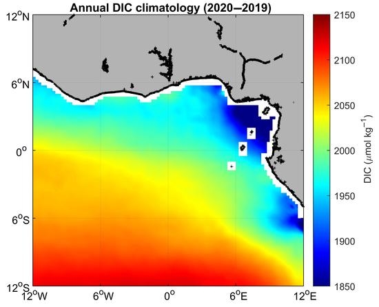
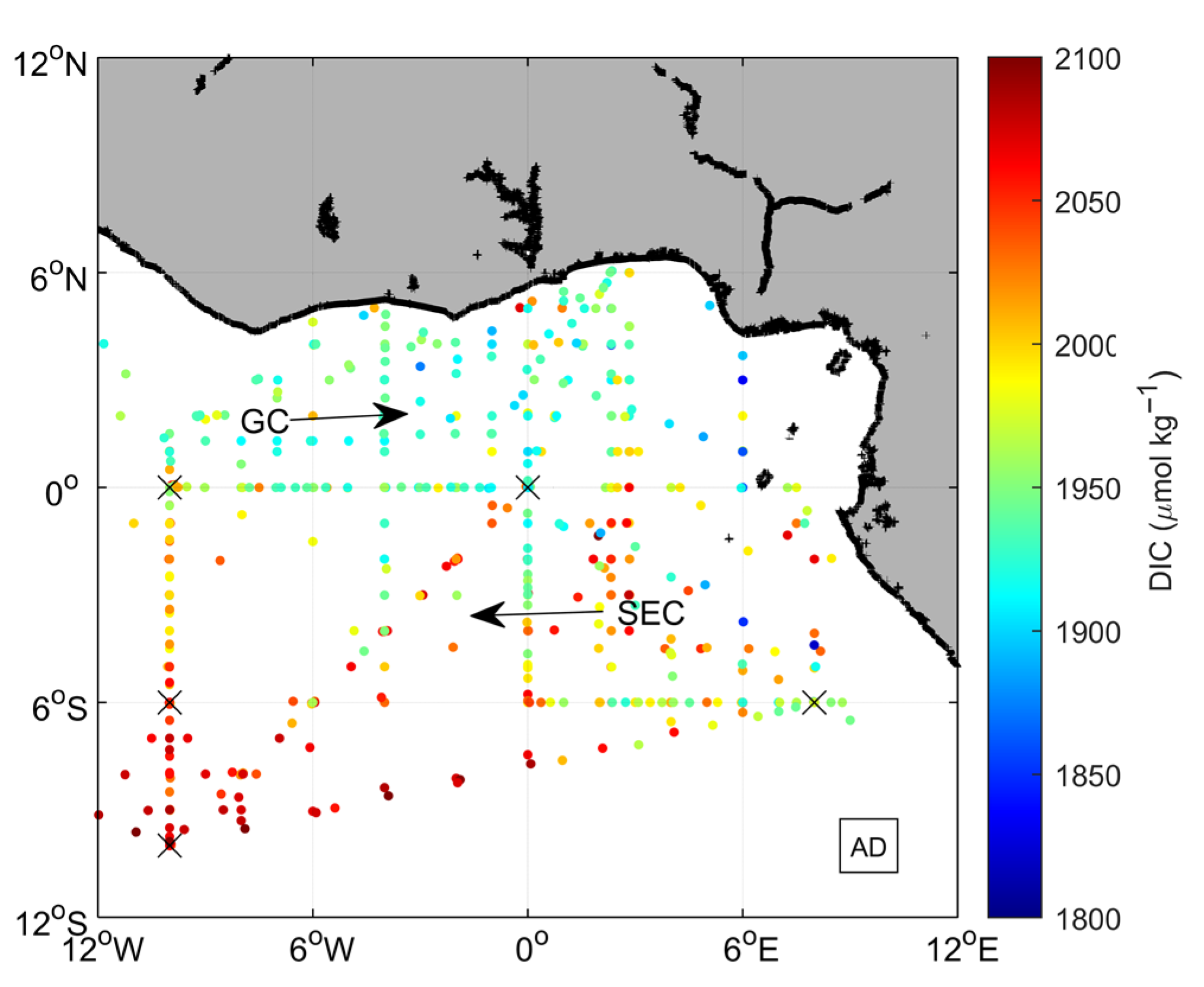
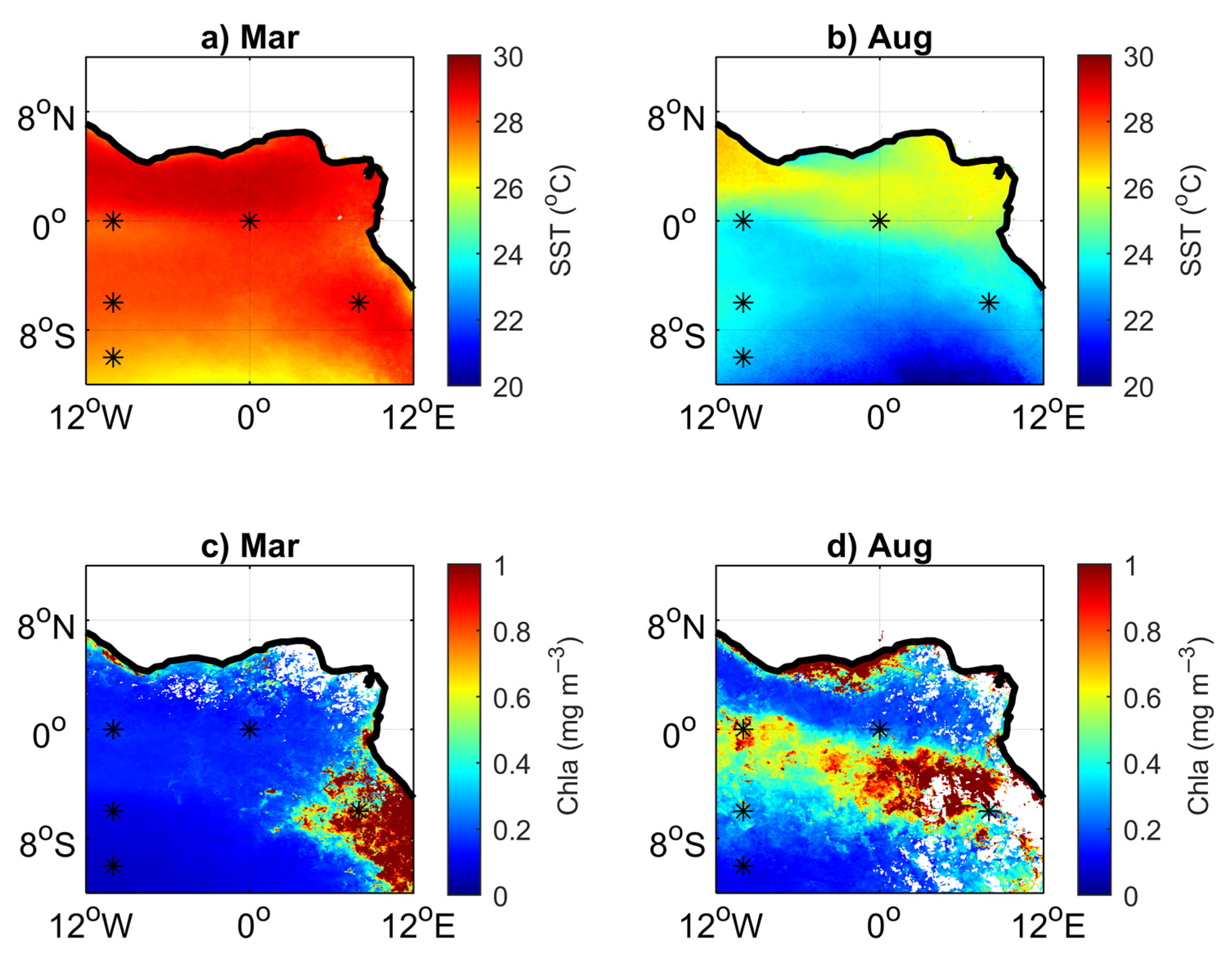
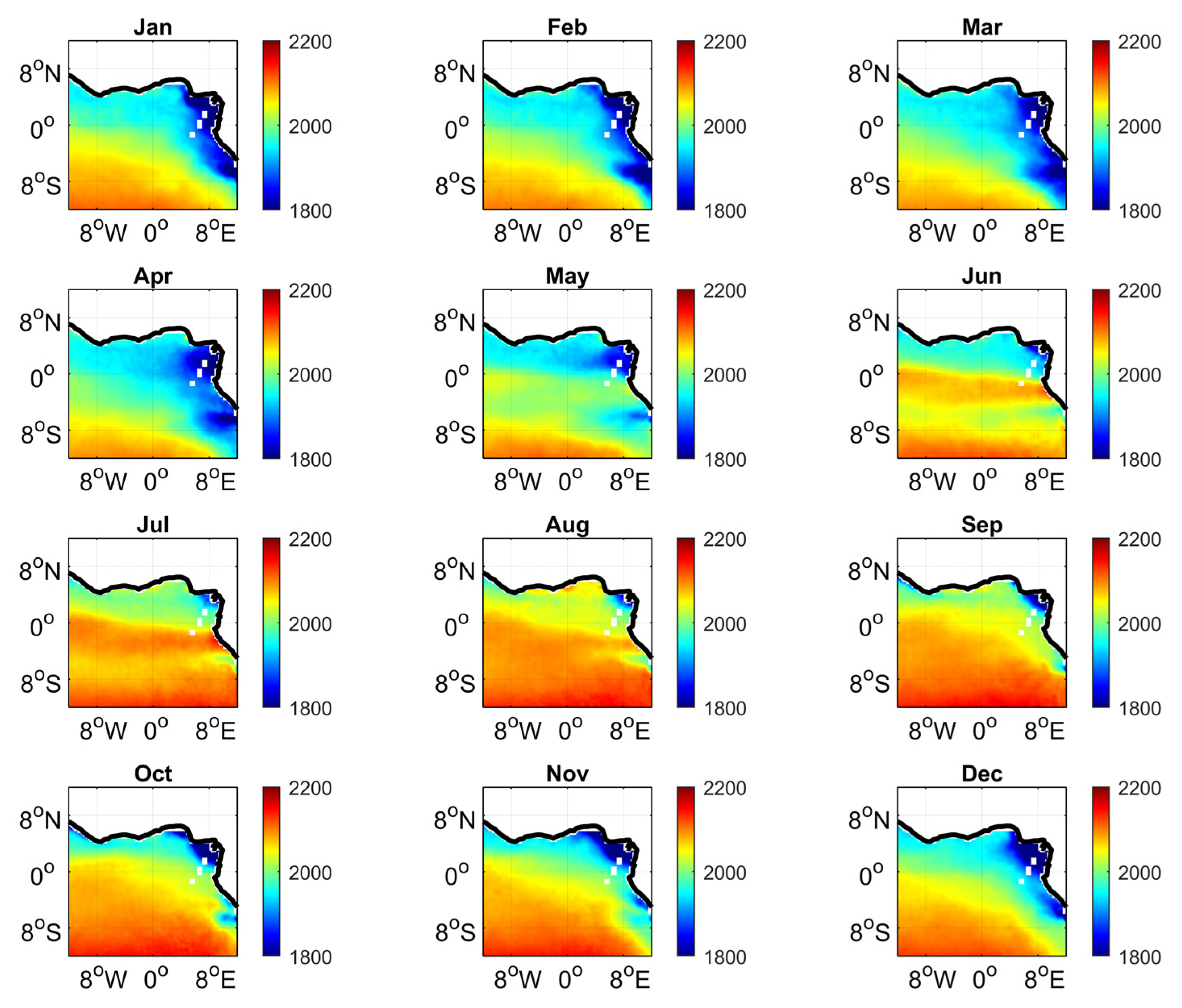
3.1. Environmental Setting

In the 12° S–12° N, 12° W–12° E region, the MODIS climatological SST varies from 24.55 °C in July to 27.01 °C in March. During the warm season, warm water spreads over most of the basin as shown for the month of March (Figure 2a). From June to September, the surface water is cooler (<25.5 °C) as the equatorial and coastal upwellings are well developed. The months of March and August are chosen to illustrate the contrasts between the two seasons (Figure 2a,b). During the cold season, a central West African upwelling occurs in the northern part of the Gulf of Guinea between approximately 8° W and 4° E, north of 2° N, from June to October [17]. The cooling is visible in the SST map of August as a small band of cooler SST along the coast (Figure 2b). Along the coast of Gabon, around 10° E near the equator, the coastal upwelling merges with the equatorial upwelling forming the Atlantic cold tongue (ACT). In the southernmost part of the basin, austral winter cooling leads to the coldest SST.
During the warm season, the productivity is low and the chlorophyll concentrations remain close to 0.2 mg m−3 except along the coastline, and in the Congo plume near 6° S, 10° E (Figure 2c). During the cold season, the chlorophyll concentrations increase along the coast, especially in the coastal upwelling of the Gulf of Guinea, and in the equatorial upwelling (Figure 2d). In the south, near 10° S, 9° E, the Angola Dome is maintained by the dynamic uplift of the thermocline, and it is also a productive region [44]. Signorini et al. [12] explain the surface distribution of the chlorophyll in the tropical Atlantic by the upwelling, defined as large vertical excursions of the thermocline, and by the river plumes. Both processes supply nutrients that lead to biological activity. Productive waters are advected by surface currents and arrive at the PIRATA moorings with the exception of the mooring at 10° S, 10° W that remains in very low chlorophyll waters throughout the year (Figure 2c, d). From 2010 to 2019, the MODIS chlorophyll concentrations during the July–September months are significantly higher than during the remaining months of the period (p-value < 0.0001), in agreement with previous studies [22]. This confirms that the cold season corresponds to the productive season.
The region is also affected by freshwater input from precipitation and river runoff. The maximum precipitation is an indicator of the position of the Intertropical Convergence Zone (ITCZ). The ITCZ migrates seasonally and is located at its northernmost position in July and at its southernmost position in March. In the ETA, the ITCZ is over the ocean during the warm season from approximately December to June. In March, it is located slightly north of the equator (Figure 3a) whereas in August it is over the land (Figure 3b). The precipitation feeds the numerous rivers that discharge into the Atlantic, which affects the distribution of SSS in the basin. The northern part of the basin is fresher than the southern part because of the presence of the ITCZ, and of the runoff of the rivers (e.g., Niger, Volta) located in the eastern Gulf of Guinea. North of about 2° N, the eastward Guinea Current, an extension of the North Equatorial Counter Current (NECC), is relatively fresh as it receives large precipitation due to the presence of the Intertropical Convergence Zone (ITCZ).
South of the equator, the areas of freshwater are located along the coastline, associated to high precipitation, and near the Congo mouth at 6° S (Figure 3). The Congo River has a bimodal hydrological cycle with its maximum river discharge in December and a secondary peak of discharge in May, whereas the minimum discharge is in August and March [45]. In March, the SSS distribution follows the precipitations with low SSS (<35) associated to high precipitation in the northern and southeastern parts of the basin (Figure 3a,c). In August, the salinity is higher and low salinity (<34) is encountered near the rivers mouths of the Volta and Niger in the north and of the Congo in the south (Figure 3d). During this month of minimum discharge, the extension of low SSS water near the Congo mouth is limited.
The physical conditions in this region show a north–south difference between warmer and fresher waters in the north and colder and saltier waters in the south because of the precipitations, river outflows and the coastal and equatorial upwellings. In the northern part of the basin, the climatological SST ranges between 25.26 °C in July and 28.82 °C in February and the SSS is below 35.2, reached in August. In the southern part, the SST varies from 22.41 °C in July to 27.41 °C in February, and the SSS varies from 35.2 in April to 35.88 in July. The north–south gradient is visible on the satellite SST throughout the year. Even during the warm season, as illustrated in March (Figure 2a), the surface water is warmer north of the equator than south of it.

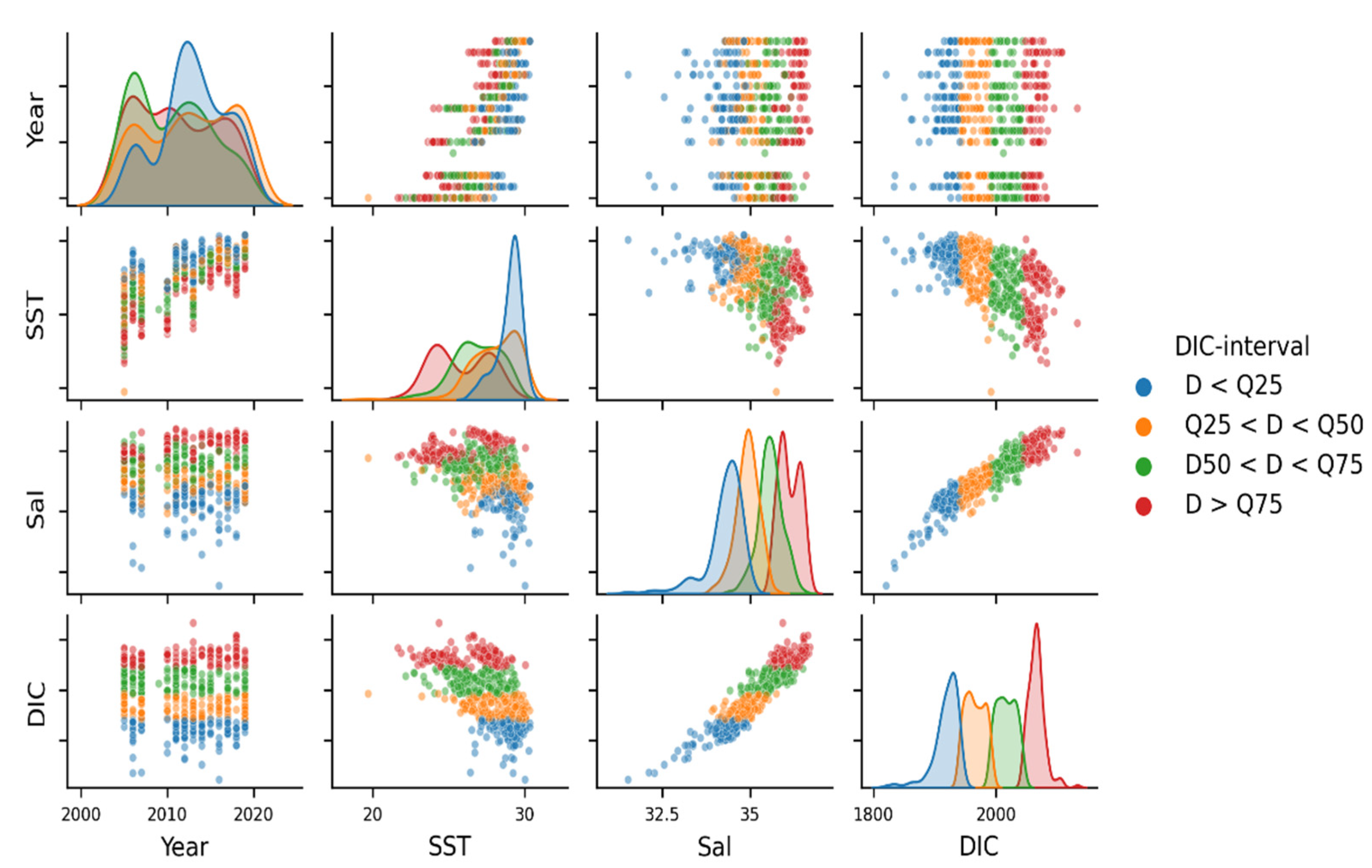
3.2. Variability and Drivers of the Carbon System

The DIC concentrations of the samples collected from 2005 to 2019, west of 10° E, range from 1618 to 2133 μ mol kg−1 with the lowest concentrations (<1800 μ mol kg−1) close to the Congo outflow and the highest (>2100 μ mol kg−1) in the southwestern part of the region. The distribution of the DIC samples highlights the lower concentrations north of the equator compared to the south (Figure 1). As TA is strongly correlated to SSS, TA exhibits also a north–south difference. In the north, TA is lower with values ranging from 2114 to 2369 μ mol kg−1 and a mean of 2278 ± 38 μ mol kg−1. In the south, TA has a mean value of 2324 ± 66 μ mol kg−1 with a maximum of 2433 μ mol kg−1 reached south of 8° S, near 4° W where evaporation dominates. The lowest TA value of 1832 μ mol kg−1 is found in the Congo plume. Warm and fresh waters are located in the GC system and exhibit lower TA and DIC concentrations whereas colder and saltier water mass transported by the SEC have higher alkalinity and DIC content. The distributions of SST, SSS, DIC and TA north and south of the equator are significantly different (p < 0.001).
DIC concentrations vary according to the main system of currents and depend on the water masses present in the region, which are characterized by their SST and SSS. This led Koffi et al. [41] to propose an empirical relationship using data over 2005–2007. However, due to the atmospheric CO2 increase and air–sea exchange, CO2 increases in the ocean over time and the relationship presents a bias. The difference between the observations and the regression increases over time, which confirms that the relationship is no longer valid for recent years. According to the atmospheric CO2 measurements during EGEE 3 and PIRATA FR-29, the atmospheric fCO2 has increased from 367.6 ± 1.7 μ atm in June 2006 to 392.2 ± 2.4 μ atm in March 2019, which corresponds to a rate of 1.9 μ atm yr−1.
In order to take into account the CO2 increase over time, we develop a new multiple linear regression (MLR) by adding a time variable:
DIC = −4585.8 (± 371.16) − 12.46 (± 0.53) ∗ SST + 54.36 (± 0.93) ∗ SSS + 2.49 (± 0.19) ∗ Year
This relationship is based on 637 samples collected in the 12° W–10° E, 10° S–10° N region from 2005 to 2019. The RMSE is 15.3 μ mol kg−1 and r2 = 0.93. The negative sign of the SST coefficient in Equation (3) reflects the contribution of the upwelling with cold SST leading to higher concentrations of DIC. The same regression is performed after normalization of the data (by subtracting the mean and dividing by the standard deviation) in order to determine the weight of each predictor. The coefficients for SST, SSS and Year are −0.42, 0.75 and 0.20, respectively. The stronger predictor is SSS, which is the dominant factor driving the DIC variations. However, without taking into account the SST, the variance explained would drop from 93% to 87% and the RMSE would increase to 21 μ mol kg−1.
Equation (3) is determined using discrete samples of DIC and needs to be validated with independent data. Surface fCO2 has been measured underway during two cruises (EGEE 3 and PIRATA FR-29) and at two moorings (6° S, 10° W and 6° S, 8° E) on an hourly basis. In order to check the robustness of Equation (3), DIC is calculated from the alkalinity–SSS relationship and the fCO2 measurements. The calculated DIC is then compared with the predicted DIC (Table 2). DIC given by Equation (3) is in good agreement with DIC calculated from underway fCO2. The correlation coefficient is always over 0.96 and the RMSE is within the uncertainty given by Equation (3). The highest RMSE is found at 6° S, 8° E.
Using monthly MODIS SST and SMOS SSS fields on a 0.25° grid, the monthly regional distribution of DIC can be estimated using Equation (3) to map its spatial variations (Figure 4). The monthly climatology of DIC is built for the January 2010 to September 2019 period. Overall, the monthly maps of DIC are similar to the SSS maps with lower values in the northern part of the basin and close to the river mouths.
Lower DIC concentrations are associated with the northern water mass and range from a mean value of 1924 μ mol kg−1 in April to 2027 μ mol kg−1 in August. Higher DIC concentrations are found in the southern water mass with a mean value of 2001 μ mol kg−1 in April to 2096 μ mol kg−1 in August. The monthly north–south DIC concentrations are significantly different throughout the year (p-value < 0.0001). During the upwelling period (July–September), the DIC concentrations are significantly higher than during the warm season (p-value < 0.0001). Thus, for the upwelling period, the mean DIC is 2070 ± 70 μ mol kg−1, whereas it is 2007 ± 28 μ mol kg−1 during the warm season over the 2010–2019 period. In the upwelling season, the north–south contrast in DIC corresponds to a north–south SST difference. For example, in August, warm surface waters (>26 °C) are separated from cold waters (<24 °C) with the frontal zone located around the equator (Figure 2b). This front is also observed on the DIC maps from June to September (Figure 4).

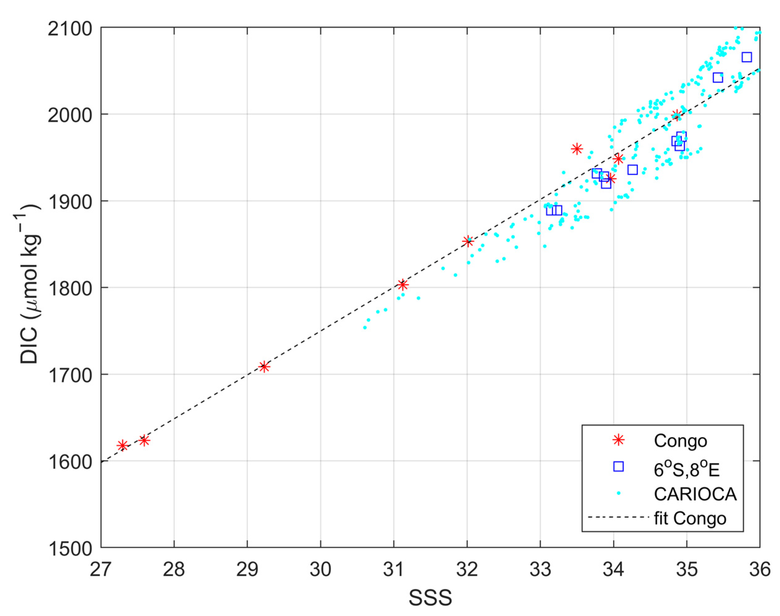
3.3. Impact of the Congo Plume

The Congo has by far the strongest river discharge in this region. Near the Congo mouth, the carbon system is affected by the Congo discharge and is examined from nine observations taken east of 10° E, around 6° S, over the period 2013–2018 from March to June. The lowest salinity (27.3 psu) was observed in March 2018, at the time of the secondary minimum of the Congo discharge. There was no sampling during the period of high Congo discharge, in December and May. Using the nine samples near the Congo outflow, the mixing between the river and oceanic waters gives the following equation:
DIC = 50.60 (± 1.97) ∗ SSS + 231.73 (± 62.19)
with a RMSE of 16.0 μ mol kg−1 and r2 = 0.99. The relationship covers the region close to the Congo mouth from 6° S to 5° S, east of 10° E. Further west, carbon data are available at the mooring at 6° S, 8° E. Hourly fCO2 has been monitored at 6° S, 8° E from 2017 to 2019 with a CARIOCA sensor. This dataset includes observations from March to August. In addition, DIC samples have been taken at this site. These DIC samples and the DIC calculated from daily averages of fCO2 and TA–SSS tend to depart from the mixing line (Figure 5). The RMSE is 32 μ mol kg−1 (N = 358) and 24 μ mol kg−1 (N = 11) for the calculated DIC and for the DIC samples at 6° S, 8° E, respectively.
The DIC data at 6° S, 8° E are better estimated by Equation (3), giving a RMSE of 14 μ mol kg−1 for both the 11 samples taken at the site and the DIC calculated from the daily fCO2. This suggests that the conservative mixing applies near the River mouth but it is no longer valid further west, at 8° E. Nevertheless, the influence of the Congo at the mooring is noticeable. Using satellite based data products, Hopkins et al. [46] show that the Congo plume extends northwest along the coastline or west-southwest into the Atlantic transported by the SEC. From MODIS chlorophyll images (Figure 2c,d), high chlorophyll concentrations are observed at the mooring at 6° S, 8° E in both seasons and originate from the coast near the Congo mouth.
Using all the available data measured at 6° S, 8° E over the 2006–2019 period, the SSS are grouped by month (Figure 6a). A data gap occurred from 2007 to 2013 as no mooring was deployed. This site exhibits large salinity variations. The lowest salinity of 30.22 psu, occurs in May 2018 during the secondary maximum discharge of the Congo. The numerous outliers usually point towards lower salinity than the median. In December, during the maximum Congo discharge, the salinity of the outliers ranges from 32 to 29 psu. The large range of salinity of the outliers (>1 psu) is usually observed around the maximum discharge periods, December and May. The median salinity of December is over 35 psu, which indicates that the plume has not reached the mooring yet, except for some years as in 2006 when a salinity close to 29 psu was observed. The lowest SSS median is in January, which suggests that the Congo plume, transported by the westward SEC, reaches the mooring. Based on satellite images, Hopkins et al. [46] found that the maximum offshore extent of the Congo plume occurs between December and April with a January peak. The freshwater supplied by the secondary peak of discharge, in May, tend to move towards the Gulf of Guinea [47]. The minimum Congo discharge occurs in August, which corresponds to the highest salinity at 6° S, 8° E. The measured values of SSS and DIC, calculated from fCO2 at the mooring in 2017, 2018 and 2019, and averaged for each month, are also indicated (Figure 6).
The DIC variations follow closely the SSS variations with the highest salinity corresponding to the highest DIC in August, the largest variations in January and the lowest DIC concentrations occurring during the January–May period (Figure 6b). The year-to-year variability is very pronounced as shown by the samples taken at this site. In April 2017, the salinity is lower than 1 psu and DIC is higher than 50 μ mol kg−1 compared to April 2018 and 2019. Likewise, in June 2018 a low salinity (34 psu) corresponds to a low DIC (1968 μ mol kg−1) whereas in June 2017 and 2019 the salinity is over 35 psu and the DIC concentrations over 2029 μ mol kg−1.
The distribution of the chlorophyll from MODIS is examined at the 6° S, 8° E mooring (Figure 7). The chlorophyll concentrations at this site are relatively high, which is in contrast with the other four PIRATA moorings where concentrations are always lower than 1.5 mg m−3 at 6° S, 10° W and lower than 3 mg m−3 at the two equatorial moorings. The lowest chlorophyll concentrations (<0.25 mg m−3) are encountered at 10° S, 10° W as this site is outside the area of influence of both the Atlantic cold tongue and the Congo plume.
At 6° S, 8° E, the highest concentrations of MODIS chlorophyll a occur in July–September and, to a lesser extent, in January–February, which is in agreement with the results of Signorini et al. (1999) using SeaWiFS (Sea-viewing Wide Field-of-view Sensor) chlorophyll a from 1997 to 1998. The concentrations of the years 2017, 2018 and 2019 are indicated (Figure 7) to compare with the DIC variations (Figure 6b). The chlorophyll a from MODIS is highly variable at 6° S, 8° E with the highest concentrations in August, as shown by the whisker reaching over 7 mg m−3 (Figure 7), when the concentrations of DIC are the highest. There is no clear link between DIC and chlorophyll concentrations as the highest chlorophyll are not associated with low DIC that would occur if strong carbon uptake were taking place. In July–September, both chlorophyll and DIC concentrations are high. This suggests that biological activity is not the dominant driver of carbon variations at this site.

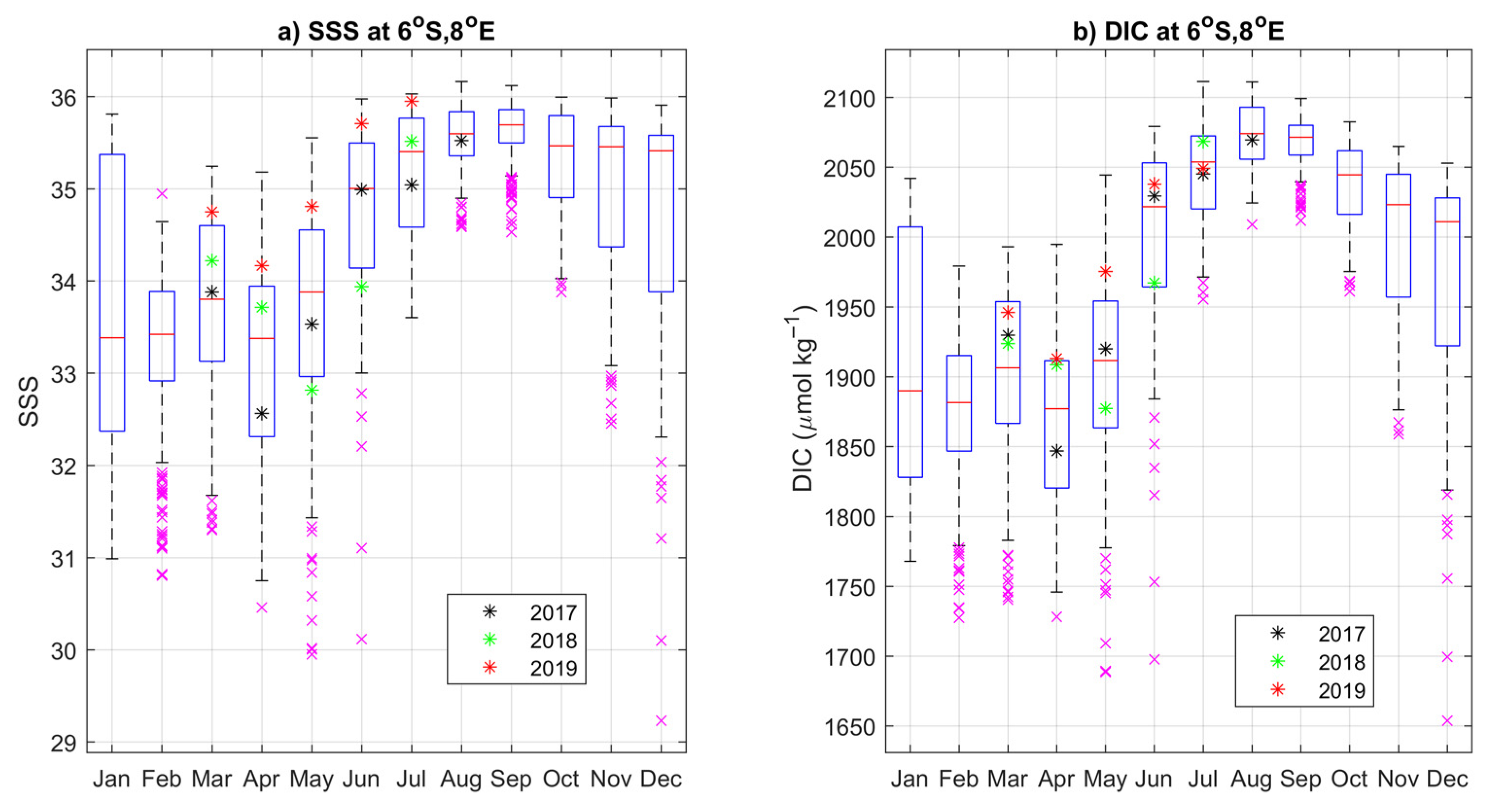
3.4. Year-to-Year Variability of the Carbon Parameters

In the ETA, the longest time-series of carbon parameters is the monitoring of hourly fCO2 at 6° S, 10° W that started in 2006. At 6° S, 8° E, the monitoring of fCO2 is rather limited with observations from 2017 to 2019 and a large data gap in 2018–2019 due to the drift of the buoy. The daily DIC at these two sites, calculated from daily fCO2, is compared with the DIC from the MLR, and with the samples taken during the PIRATA cruises at both locations (Figure 8a, b). The MLR reproduces rather well the variations of DIC at 6° S, 10° W but overestimates the DIC concentrations in some years, such as in July–September 2011 where the difference is over 35 µmol kg1. The timing of the decreases and increases in DIC is in good agreement between the DIC calculated by the MLR and the DIC calculated from underway fCO2. At 6° S, 10° W, DIC values are higher in July–November and lower in April–June each year. At 6° S, 8° E the daily variations of DIC tend to show the lowest concentrations in April and the highest in August but with large variations. For example, DIC concentrations vary by more than 150 µmol kg1 within days in April 2017 (Figure 8b). In April 2019, the lowest DIC is much higher than in April 2017 with a difference reaching 125 µmol kg1. Nevertheless, the MLR captures well the high frequency variations of DIC.
As expected, given the discrepancy observed in the daily variations, monthly DIC derived from satellite data tend to give higher concentrations than DIC calculated with the PIRATA data but reproduce the seasonal variations of DIC (Figure 8c,d). The monthly DIC smooth significantly the variations. It is especially visible at 6° S, 8° E on the MLR with a reduced range of variations of DIC, decreasing from 460 to 320 μmol kg1. The seasonal cycle of DIC at 6° S, 8° E is more distinct than on the daily variations. Given that the satellite pixels correspond to a much larger area than the observations at the mooring, there is expected discrepancy between the two products but overall, the MLR reproduces well the seasonal cycle and the year-to-year variations of DIC.
After verifying the DIC variations over time at the two sites where observations are available, we examine the monthly DIC variations given by the MLR using satellite data at regional scale. The DIC concentrations are lower in the north than in the south with the maximum values occurring from July to September each year in both regions (Figure 9). The monthly means of DIC over the entire region are closer to the DIC variations observed in the south in Figure 9 because the region north of the equator includes a large section of land and, hence, the weight of this region is much smaller in the global average. The lowest concentrations of DIC occur in March–April in the south, whereas, north of the equator, low DIC concentrations (<1950 μmol kg1) occur over a much longer period, usually from November to May. The difference between the highest and the lowest DIC concentrations range from about 80 to 125 μmol kg1 in both regions. This range is much higher than the year-to-year variability of DIC that is less than 50 μmol kg1 over the 2010–2019 period. On annual average, over the whole region, the DIC variations are less than 35 μmol kg1. In both the northern and southern regions, the seasonal variability is responsible for the large variations of DIC (Figure 9).
The year 2010 exhibits the lowest annual average of DIC in the north (p-value = 0.006) and in the south but, in the southern region, it is not significantly different from the other years. The salinity data retrieved from SMOS are of lower quality from January to March 2010, at the beginning of the series. If we remove these 3 months in the time series, the annual mean of DIC in 2010 is no longer significantly different from the other years in both regions. The highest DIC annual average occurs in 2015 north of the equator and in 2017 south of it, but these years are not significantly different from the other years. Overall, the year-to-year variability of DIC does not highlight any anomalous year over the 2010–2019 period.

4. Discussion

4.1. Main Features of the Carbon Parameters

Both DIC and TA are strongly correlated to physical parameters. The TA–SSS relationship is robust and does not vary much with new observations. The DIC can be estimated by taking into account the water masses, characterized by their temperature and salinity, and an increase in oceanic surface CO2 over time due to the atmospheric CO2 increase. In stratified regions, like the tropics, the oceanic CO2 tends to follow the rate of the atmospheric increase. The MLR used here shows that SSS, SST and year describe well the DIC variations in this region. Other methods, taking into account non-linear processes, do not perform significantly better than the MLR (Appendix A), which implies that the DIC dependency on the SSS, SST, and the year is essentially linear. However, feed forward neural networks show slightly better results with values of the first and last quantiles of DIC, suggesting that a non-linear dependency exists between DIC and input variables (Appendix A). Low concentrations of DIC are mostly encountered in coastal area in river plumes. As most samples are in the open ocean region, the MLR is adequate here. However, a non-linear method would be required when more samples in the coastal zone become available.
The DIC distribution in the 12° W–10° E, 12° S–12° N region (Figure 4) shows high DIC concentrations in most part of the ETA during the upwelling season. Overall, the DIC values range from 1945 to 2090 μ mol kg−1 with an average of 2024 ± 37 μ mol kg−1 from 2010 to 2019. The highest DIC values occur during the cold and productive season, in July–September each year (Figure 9). In this season, the MODIS chlorophyll is significantly higher. The vertical supply of subsurface waters is responsible for bringing CO2-rich waters to the surface that spread over the basin. It is the dominant process and the biological activity is not strong enough to counterbalance the carbon supply.
The DIC concentrations in the ETA are similar to DIC observations collected further west. In the Western Tropical Atlantic, in the SEC, DIC concentrations average 2045 ± 40 μ mol kg−1 in April–September and 2058 ± 22 μ mol kg−1 in October–March from analyses made over the period 1989–2014 [48]. In the ETA, south of the equator, the DIC concentrations, between 2010 and 2019, average 2059 ± 39 μ mol kg−1 in April–September and 2036 ± 32 μ mol kg−1 in October–March.
The lowest DIC concentrations in the ETA are observed east of 10° E near the Congo mouth. In this area, DIC is better estimated with the conservative mixing Equation (4) than with the MLR. The slope of Equation (4) is different from the ones given by published relationships (Table 3). As previously noticed [49], the value of the slope is sensitive to the salinity range. Using all the data or data with salinity higher than 33 changes the slope from 46.5 μ mol kg−1/psu to 50.6 μ mol kg−1/psu [49]. It also changes the end-member (DIC at SSS = 0) for the Congo from 355 ± 48 μ mol kg−1 to 221 ± 97 μ mol kg−1. As no sample was taken during the highest Congo discharge, our lowest salinity is above 27. Nevertheless, the end-member for the Congo River of 231.7 ± 62.2 μ mol kg−1 is in good agreement with the average riverine DIC concentrations of 258 ± 29 μ mol kg−1 measured at Brazzaville–Kinshasa by [45].
TA values are also lower near the Congo mouth and are better estimated by the following equation than by Equation (2):
TA = 61.89 (± 0.70) ∗ SSS + 137.51 (± 22.08)
which gives a TA end-member of 137.51 ± 22.08 μ mol kg−1, in agreement with the riverine TA values ranging from 85 to 235 μ mol kg−1, the variations being strongly dependent on the Congo discharge unlike the DIC end-member that is relatively constant [45].
The chlorophyll images show the high biological activity near the Congo mouth, which decreases DIC concentrations and leads to carbon uptake as previously proved by the estimates of the CO2 flux in this region [13,14]. The mouth of the Congo is located at 6° S, 12.3° E and its plume can be traced 400 to 1000 km from the mouth. The influence of the Congo plume is evidenced at 6° S, 8° E by the large salinity (Figure 6a) and chlorophyll variations (Figure 7), as well as the spatial distributions of chlorophyll (Figure 2c,d) and salinity (Figure 3c,d). In order to relate the DIC distribution (Figure 4) to the chlorophyll climatology, the chlorophyll fields were re-gridded on a 0.25-degree map and the correlation between DIC and chlorophyll concentrations was calculated at each grid point from January to December (Figure 10).
The blue regions correspond to negative correlations and coincide with high chlorophyll concentrations and low DIC, which are caused by carbon uptake. The positive correlations (in red) correspond to regions where chlorophyll and DIC follow the same seasonal cycle. In the equatorial upwelling region, high DIC and high chlorophyll concentrations are observed during the upwelling season (July–September) and lower concentrations occur during the rest of the year, which explains the positive correlation between DIC and Chla. Outside the upwelling region, low chlorophyll concentrations are observed but follow the seasonal cycle and the DIC–Chla correlation is also positive. Near river outflows, high chlorophyll concentrations are usually associated with low SSS and low DIC concentrations leading to negative DIC–Chla correlations. The spatial extension of the negative correlations indicates the areas of influence of the river discharge. As SSS is a strong driver of DIC variations in the ETA, the negative DIC–Chla correlations correspond to areas with low SSS and high chlorophyll concentrations.
At 6° S, 8° E, low DIC and TA are observed especially in March–April during the period of maximum offshore extension of the Congo plume [46]. Nevertheless, the DIC observations at this site are better reproduced by the MLR, which suggests rapid mixing of the plume with oceanic waters during its westward propagation.
Observations made at 6° S, 8° E are compared with those at 6° S, 10° W. Unfortunately, measurements of fCO2 are available at both sites for 6 months only, from March to August 2017. The CO2 flux is much lower at 6° S, 8° E than at 6° S, 10° W (Table 4). However, the difference of fCO2 between the ocean and the atmosphere, ΔfCO2, is similar at both sites. DIC and SSS, and hence TA, are significantly lower at 6° S, 8° E. An increase in DIC would increase fCO2 but the increase in TA would decrease fCO2. The increase in DIC from 6° S, 8° E to 6° S, 10° W is compensated by the increase in alkalinity, so that overall, the mean fCO2 (and ΔfCO2) remains similar to the mean fCO2 at 6° S, 8° E.
The flux is significantly lower at 6° S, 8° E because the wind speed is much weaker close to the coast than offshore. However, the CO2 flux remains positive with only slight negative values, or close to zero, that may occur in March–April in some years (Figure 10). The flux and the ΔfCO2 are strongly correlated at this site (r = 0.95). During this time, the offshore spatial extension of the Congo plume is maximum [46] and the SSS at 6° S, 8° E is low (Figure 6a). The surface waters coming at the mooring are from the Congo plume and have low CO2 content because of the biological activity near the Congo mouth and the low CO2 content of the Congo waters. Although DIC–TA is the worst pair to calculate fCO2, the flux has been reconstructed at 6° S, 8° E to examine its annual variations (Figure 11, MLR sat). Some differences can reach more than 2 mmol m−2 d−1 as in June 2017 but the reconstruction suggests that the site is a source of CO2 with some possible CO2 uptake occurring during the first months of the year.

4.2. Year-to-Year Variability

Using the MLR and the SST and SSS satellite fields from 2010 to 2019 at regional scale, the anomalies of DIC are calculated and compared with the anomalies of the physical parameters (Figure 12). As salinity is a strong predictor of DIC, the monthly variations of DIC anomalies from 2010 to 2019 are correlated with SSSA (r = 0.87). The anomalies of DIC are negatively correlated with SSTA and the correlation is much weaker (r = −0.38). The anomalies of SST in the ETA are related to the TSA index that cover a much larger area of the South Atlantic (30° W–10° E, 20° S–0°), with a correlation coefficient between SSTA and TSA of 0.77.
In the tropical region, the year 2010 is characterized by much warmer temperatures whereas 2012 is a cold year [50]. The positive SSTA in 2010 are observed in the northern Tropical Atlantic and affect the air–sea CO2 flux [51]. In the ETA, SSTA are close to zero suggesting that the anomalous conditions of 2010 are limited to the Northern Tropical Atlantic. However, the ETA presents negative SSS anomalies throughout the year 2010 that result in negative DIC anomalies (Figure 12a). There was no anomaly of precipitation in the ETA in 2010 but, during the first months of 2010, the position of the ITCZ in the tropical Atlantic remained north of the equator instead of migrating south of it. As the ITCZ is associated with high precipitations, lower-than-usual salinities advected by the NECC might explain the negative SSSA in the ETA. When comparing the SSS anomalies in 2010 north and south of the equator, the SSSA are significantly lower north of the equator (mean of −0.36) than south of it (mean of −0.16, p-value = 0.0024). Nevertheless, the impact of the SSSA anomalies on DIC is moderate as it does not exceed 40 μ mol kg−1, which is much less than the seasonal DIC variations in this region, as shown, for example, in Figure 9.
The other strong anomaly in the tropical Atlantic is the cold event of 2012 mainly observed in the northeastern Atlantic and the southern hemisphere [50]. From November 2011 to early 2012, a strong cooling anomaly (SSTA < 0) occurs in the region and is associated with a negative TSA index (Figure 12b). The distribution of fCO2 at 6° S, 10° W was affected by the cooling with a decrease in fCO2 associated to a decrease in SST during January–March 2012 compared to other years [52]. However, the SST variations have a moderate effect on DIC and this cooling anomaly does not affect much the DIC concentrations (Figure 12a).
According to [2], interannual fCO2 is mainly driven by SST in the equatorial Atlantic extending from 50° W to 5° E and by DIC in the equatorial Pacific. The fCO2 monitoring is still sparse in the tropical Atlantic to conclude. Nevertheless, the interannual events of 2010 and 2012 affected fCO2 and suggest an important role of SST anomalies whereas in the ETA, DIC is mainly driven by SSS variations. The use of DIC and TA to calculate fCO2 does not reproduce well the fCO2 variations observed at 6° S, 10° W, which might be explained by the strong co-variation of fCO2 and SST. Using pH that has a strong dependency with SST with either DIC or TA would better reproduce observed fCO2. Monitoring fCO2 and calculating TA, with the robust TA–SSS relationship, allow the calculation of pH. This would be a substitute for direct pH measurements. Given the strong seasonality of carbon parameters in this region, long term monitoring is necessary to be able to quantify the acidification rate in this region.

5. Conclusions

The DIC distribution has been examined in the ETA (12° W–12° E, 12° S–12° N) as well as the factors controlling its distribution. DIC strongly depends on the water masses and increases over time due to the atmospheric CO2 increase. In the northern part of the basin, relatively fresh and warm waters are associated with lower DIC concentrations compared to the southern part where colder and saltier waters are enriched in CO2. A multiple linear regression between DIC and SST, SSS and year has been determined with SSS as the main predictor of DIC. Other regression techniques, such as decision tree, random forest and feed forward neural networks, do not significantly improve the DIC estimation except for low DIC concentrations corresponding to coastal data. However, a neural network would be required when more coastal data become available as non-linearity occurs at low values.
East of 10° E, the strong influence of the Congo plume is evidenced with a different relationship which corresponds to conservative mixing between the river and oceanic waters. The end-members of 231.7 ± 62.2 μ mol kg−1 for DIC and 137.5 ± 22.1 μ mol kg−1 for TA are in good agreement with published riverine measurements. The Congo plume reaches its more offshore spatial extension during December–April and affects the distribution of DIC at the 6° S, 8° E mooring. Nevertheless, the conservative mixing is no longer valid as the plume rapidly mixes with oceanic waters. Consequently, the carbon uptake is restricted to the region close to the Congo mouth and the carbon supplied by the upwelling season is the dominant process in the ETA. The seasonal cycle dominates the variations of DIC in the region, whereas the year-to-year variability of DIC is less than 40 μ mol kg−1 over the 2010–2019 period. SSS is the main driver of DIC in this region and the cold event of 2012 does not lead to significant DIC anomalies.
Although no pH measurements are made, the observations of fCO2 and the calculation of TA from SSS allow the calculation of pH. Pursuing the monitoring of fCO2 at time-series stations will contribute to the quantification of the rate of ocean acidification in this region.

Author Contributions

Conceptualization, N.L.; methodology and validation, N.L., C.M. and D.K.; writing—original draft preparation, N.L.; writing—review and editing, N.L., C.M., D.K., L.B. and U.K. All authors have read and agreed to the published version of the manuscript.

Funding

This research was funded by the Institut de Recherche pour le Développement (IRD), the European integrated project AtlantOS (grant agreement 633211), and the French Integrated Carbon Observation System (ICOS-France).

Data Availability Statement

The data presented in this study are openly available and the references are given in the paper.

Acknowledgments

We are very grateful to the volunteers who collected the samples during the PIRATA cruises and to the US IMAGO from the IRD, especially F. Roubaud, J. Grelet and P. Rousselot for the installation and deployments of the CO2 sensors. DIC and TA have been analyzed at the service national d’analyses des paramètres océaniques du carbone in LOCEAN. The L3_DEBIAS_LOCEAN_v4 Sea Surface Salinity maps have been produced by LOCEAN/Institut Pierre Simon Laplace (UMR CNRS/UPMC/IRD/MNHN) laboratory and ACRI-st company that participate in the Ocean Salinity Expertise Center (CECOS) of Centre Aval de Traitement des Donnees SMOS (CATDS). This product is distributed by the Ocean Salinity Expertise Center (CECOS) of the CNES-IFREMER Centre Aval de Traitement des Donnees SMOS (CATDS), at IFREMER, Plouzane (France). We thank two anonymous reviewers for their constructive comments.

Conflicts of Interest

The authors declare no conflict of interest.

Appendix A. Regression Methods and Results

Four data-driven regression methods (Multiple Linear Regression, Decision Tree, Random Forest and Feed Forward Neural Networks) have been applied to estimate DIC in the Eastern Tropical Atlantic. Figure A1 presents the dataset with the relationships between DIC and the predictors (SST, SSS and Year) and the distribution divided by DIC quantiles (in color).
Figure A1. Scatter plots between variables and density plots for each variable (on the main diagonal). Data are colored according to the intervals of the quantiles of DIC (25%, 50%, 75%).
Oceans 02 00008 g0a1
Decision Trees (DT) are a non-parametric supervised learning method used for classification and regression. The goal is to create a model that predicts the value of a target variable by learning simple decision rules inferred from the data features. During the tree construction, the dataset is iteratively split by the parameters maximizing the variance of the predicted variable.
Random Forest (RF) algorithms are ensemble methods using so called perturb-and-combine techniques [53] designed for decision trees. This means a diverse set of regressors is created by introducing randomness in the model construction. The prediction of the ensemble is given as the averaged prediction of the individual regressors. Each tree in the ensemble is built from a sample drawn with replacement (i.e., a bootstrap sample) from the training set. In addition, when splitting each node during the construction of a tree, the best split is found either from all input features or a random subset of a predefined size.
Feed forward neutral networks (NN) are part of artificial neural networks. NN are non-linear functions able to uniformly approximate a wide class of functions encountered in physics [54], which include continuous and derivable functions with respect to each variable. The minimization used allows a global optimization of the set of parameters. Feed forward neural networks are a broadly applied technique in classification and regression tasks. Table A1 summarizes the characteristics of the feed forward Neural model. We use keras API [55] in Python using TensorFlow [56] as back-end.
Table A1. Characteristics of the neutral networks (NN).
Meta-ParametersSpecifications
Input variablesYear, SST, SSS, SinDoY, CosDoY
Output variablesDIC
Train/ValDIC 4 quantiles (1/6 for Val from each quant.)
NormalizationCenter-reduction (both Input and Output)
Architecture Layers size: Input: 5, Hidden: 15, Output: 1
The relationship between the DIC and its potential predictors, such as the sea surface salinity (SSS), sea surface temperature (SST), the interannual trend (expressed by the year variable) have been explored using four regression models and four independent observation datasets.
For the NN, the intra-annual variations were taken into account by adding two variables: sinDoY and cosDoY, representing the sine and cosine of the day of the year, respectively, normalized between 0 and 2π. Having a validation dataset is fundamental to avoid overfitting on trained data. From the data available for training, i.e., the DIC (2005–2019), two datasets were created for training and validation processes. We applied the following method to get a homogeneous representation of data in the validation dataset: the 637 measurements of DIC (2005–2019) were separated into 4 groups according to the 25%, 50%, 75% quantiles of DIC (this corresponds to the 1941.1 μmol kg−1, 1992.2 μmol kg−1 and 2044.6 μmol kg−1 DIC values). Finally, data in each group were sorted by SST and a sample was chosen for validation, leaving the rest for training. Best results were obtained by selecting one data out of six. The sizes of these datasets are given in Table A2.
Table A2. Data distribution for the NN showing the total number of data (N), the number of data for training (NTrain) and for validation (NVal) according to the 25%, 50%, 75% quantiles (Q25, Q50, Q75) of the DIC. The corresponding values of DIC are indicated in μmol kg−1.
ConditionNNTrainNVal
DIC < Q25DIC < 1941.1159132 27
Q25 < DIC < Q501941.1 ≤ DIC < 1992.215913227
Q50 < DIC < Q751992.2 ≤ DIC < 2044.6158132 26
DIC > Q75DIC ≥ 2044.616113527
The NN is then compared with the MLR using the same groups of data (Table A3). The two methods give similar RMSE but the NN tends to perform better than the MLR for low DIC values.
Table A3. RMSE for each DIC interval for both MLR and NN methods tested on the two time-series stations and the two cruises.
Mooring or Cruise Regression MethodDIC < Q25Q25 < DIC < Q50Q50 < DIC < Q75DIC > Q75
RMSE
[µmol kg−1]
RMSE
[µmol kg−1]
RMSE
[µmol kg−1]
RMSE
[µmol kg−1]
6° S, 10° WMLRNaN13.87.27.8
NNNaN13.47.37.0
6° S, 8° EMLR18.015.012.79.4
NN14.015.011.58.9
EGEE 3MLR7.18.312.518.1
NN4.87.59.914.1
PIRATA-FR-29MLR11.28.14.86.9
NN8.111.15.39.2
The different methods, MLR, NN, DT and RF are compared without separating the data into groups (Table A4). The NN usually performs slightly better than the other methods but, as it does not lead to significant improvement, we use the MLR, which is the simplest method. This also means that the dependencies of the DIC on its main predictors, SSS, SST, and year, are mostly linear. Among these features, the SSS has the largest impact. For random forests and decision trees, the relative importance of SSS is more than 90% (up to 95% for 6° S, 10° W), while that of the SST is about 5% (calculated as total variance reduction brought by the corresponding variable).
Table A4. Same as Table 2, but including a comparison between the multiple linear regression (MLR), the decision tree (DT), the random forest (RF) and the feed forward neural networks (NN) methods.
Mooring or CruiseRegression MethodRMSE
( μ mol kg−1)
rNTime Period
6° S, 10° WMLR7.70.9666112006–2017
DT14.10.87
RF9.80.94
NN7.30.97
6° S, 8° EMLR14.80.982392017–2019
DT250.95
RF240.95
NN12.80.99
EGEE 3MLR11.80.9768952006
DT140.96
RF100.98
NN9.30.98
PIRATA FR-29MLR8.10.9944622019
DT110.98
RF90.98
NN9.40.99
Although not very different, the DT is slightly less efficient than the other methods. The DT tend to group the predicted values into clusters, due to relatively small tree depths and consequently small numbers of leaves (i.e., discrete cases with observations attributed to them). DTs typically exhibit high variance and tend to lead to overfitting. RFs decrease the variance of the ensemble estimator. By taking an average of tree predictions, with injected randomness, some errors can cancel out. In our examples RF yield slightly better results that DT for all stations, in most cases being close to the MLR model. Nevertheless, all methods used here give similar results.

References

  1. Le Quéré, C.; Orr, J.C.; Monfray, P.; Aumont, O.; Madec, G. Interannual variability of the oceanic sink of CO2 from 1979 through 1997. Glob. Biogeochem. Cycles 2000, 14, 1247–1266. [Google Scholar] [CrossRef]
  2. Wang, X.; Murtugudde, R.; Hackert, E.; Wang, J.; Beauchamp, J. Seasonal to decadal variations of sea surface pCO2 and sea-air CO2 flux in the equatorial oceans over 1984–2013: A basin-scale comparison of the Pacific and Atlantic Oceans. Glob. Biogeochem. Cycles 2015, 29, 597–609. [Google Scholar] [CrossRef]
  3. Cooley, S.R.; Coles, V.J.; Subramaniam, A.; Yager, P.L. Seasonal variations in the Amazon plume-related atmospheric carbon sink. Glob. Biogeochem. Cycles 2007, 21. [Google Scholar] [CrossRef] [Green Version]
  4. Cooley, S.R.; Yager, P.L. Physical and biological contributions to the western tropical North Atlantic Ocean carbon sink formed by the Amazon River plume. J. Geophys. Res. 2006, 111. [Google Scholar] [CrossRef] [Green Version]
  5. Subramaniam, A.; Yager, P.L.; Carpenter, E.J.; Mahaffey, C.; Björkman, K.; Cooley, S.; Kustka, A.B.; Montoya, J.P.; Sañudo-Wilhelmy, S.A.; Shipe, R.; et al. Amazon River enhances diazotrophy and carbon sequestration in the tropical North Atlantic Ocean. Proc. Natl. Acad. Sci. USA 2008, 105, 10460–10465. [Google Scholar] [CrossRef] [PubMed] [Green Version]
  6. Ternon, J.F.; Oudot, C.; Dessier, A.; Diverrès, D. A seasonal tropical sink for atmospheric CO2 in the Atlantic Ocean: The role of the Amazon River discharge. Mar. Chem. 2000, 68, 183–201. [Google Scholar] [CrossRef]
  7. Körtzinger, A. A significant sink of CO2 in the tropical Atlantic Ocean associated with the Amazon River plume. Geophys. Res. Lett. 2003, 30, 2287. [Google Scholar] [CrossRef] [Green Version]
  8. Lefèvre, N.; Flores, M.M.; Gaspar, F.L.; Rocha, C.; Jiang, S.; Araujo, M.; Ibánhez, J.S.P. Net heterotrophy in the Amazon continental shelf changes rapidly to a sink of CO2 in the outer Amazon plume. Front. Mar. Sci. 2017, 4, 278. [Google Scholar] [CrossRef] [Green Version]
  9. Ibánhez, J.S.P.; Araujo, M.; Lefèvre, N. The overlooked tropical oceanic CO2 sink. Geophys. Res. Lett. 2016, 43, 3804–3812. [Google Scholar] [CrossRef] [Green Version]
  10. Ibánhez, J.S.P.; Diverrès, D.; Araujo, M.; Lefèvre, N. Seasonal and interannual variability of sea-air CO2 fluxes in the tropical Atlantic affected by the Amazon River plume. Glob. Biogeochem. Cycles 2015, 29, 1640–1655. [Google Scholar] [CrossRef]
  11. Chao, Y.; Farrara, J.D.; Schumann, G.; Andreadis, K.M.; Moller, D. Sea surface salinity variability in response to the Congo river discharge. Cont. Shelf Res. 2015, 99, 35–45. [Google Scholar] [CrossRef]
  12. Signorini, S.R.; Murtugudde, R.G.; McClain, C.R.; Christian, J.R.; Picaut, J.; Busalacchi, A.J. Biological and physical signatures in the tropical and subtropical Atlantic. J. Geophys. Res. Ocean. 1999, 104, 18367–18382. [Google Scholar] [CrossRef] [Green Version]
  13. Bakker, D.C.E.; De Baar, H.J.W.; De Jong, E. Dissolved carbon dioxide in tropical East Atlantic surface waters. Phys. Chem. Earth 1999, 24, 399–404. [Google Scholar] [CrossRef] [Green Version]
  14. Lefèvre, N. Low CO2 concentrations in the Gulf of Guinea during the upwelling season in 2006. Mar. Chem. 2009, 113, 93–101. [Google Scholar] [CrossRef]
  15. Caniaux, G.; Giordani, H.; Redelsperger, J.-L.; Guichard, F.; Key, E.; Wade, M. Coupling between the Atlantic cold tongue and the West African monsoon in boreal spring and summer. J. Geophys. Res. 2011, 116. [Google Scholar] [CrossRef]
  16. Hisard, P. Variations saisonnières à l’équateur dans le golfe de Guinée. Cah. ORSTOM Sér. Océanograph. 1973, 11, 349–358. [Google Scholar]
  17. Hardman-Mountford, N.J.; McGlade, J.M. Seasonal and interannual variability of oceanographic processes in the Gulf of Guinea: An investigation using AVHRR sea surface temperature data. Int. J. Remote Sens. 2003, 24, 3247–3268. [Google Scholar] [CrossRef]
  18. Herbland, A.; Le Borgne, R.; Le Bouteiller, A.; Voituriez, B. Structure hydrologique et production primaire dans l’Atlantique tropical oriental (Hydrological structure and primary production in the eastern tropical Atlantic Ocean). Océanograph. Trop. 1983, 18, 249–293. [Google Scholar]
  19. Djagoua, É.V.; Affian, K.; Larouche, P.; Saley, B. Variabilité saisonnière et interannuelle de la chlorophylle en surface de la mer sur le plateau continental de la Côte d’Ivoire à l’aide des images de SeaWiFS de 1997 à 2004. Télédétection 2006, 6, 143–151. [Google Scholar]
  20. Nieto, K.; Mélin, F. Variability of chlorophyll-a concentration in the Gulf of Guinea and its relation to physical oceanographic variables. Prog. Oceanogr. 2017, 151, 97–115. [Google Scholar] [CrossRef]
  21. Abe, J.; Brown, B.; Ajao, E.A.; Donkor, S. Local to regional polycentric levels of governance of the Guinea Current Large Marine Ecosystem. Environ. Dev. 2016, 17, 287–295. [Google Scholar] [CrossRef]
  22. Radenac, M.H.; Jouanno, J.; Tchamabi, C.C.; Awo, M.; Bourlès, B.; Arnault, S.; Aumont, O. Physical drivers of the nitrate seasonal variability in the Atlantic cold tongue. Biogeosciences 2020, 17, 529–545. [Google Scholar] [CrossRef] [Green Version]
  23. Jouanno, J.; Marin, F.; Du Penhoat, Y.; Molines, J.M.; Sheinbaum, J. Seasonal Modes of Surface Cooling in the Gulf of Guinea. J. Phys. Oceanogr. 2011, 41, 1408–1416. [Google Scholar] [CrossRef] [Green Version]
  24. Voituriez, B.; Herbland, A. Etude de la production pélagique de la zone équatoriale de l’Atlantique à 4oW: I—Relations entre la structure hydrologique et la production primaire. Cah. ORSTOM. Sér. Océanograph. 1977, 15, 313–331. [Google Scholar]
  25. Christian, J.R.; Murtugudde, R. Tropical Atlantic variability in a coupled physical–biogeochemical ocean model. Deep Sea Res. Part II Top. Stud. Oceanogr. 2003, 50, 2947–2969. [Google Scholar] [CrossRef]
  26. Andrié, C.; Oudot, C.; Genthon, C.; Merlivat, L. CO2 fluxes in the tropical Atlantic during FOCAL cruises. J. Geophys. Res. 1986, 91, 11741–11755. [Google Scholar] [CrossRef] [Green Version]
  27. Oudot, C.; Ternon, J.F.; Lecomte, J. Measurements of atmospheric and oceanic CO2 in the tropical Atlantic: 10 years after the 1982–1984 FOCAL cruises. Tellus 1995, 47, 70–85. [Google Scholar] [CrossRef] [Green Version]
  28. Parard, G.; Lefèvre, N.; Boutin, J. Sea water fugacity of CO2 at the PIRATA mooring at 6oS, 10oW. Tellus B 2010, 62, 636–648. [Google Scholar] [CrossRef]
  29. Lefèvre, N.; Veleda, D.; Araujo, M.; Caniaux, G. Variability and trends of carbon parameters at a time series in the eastern tropical Atlantic. Tellus B 2016, 68, 1147. [Google Scholar] [CrossRef] [Green Version]
  30. Bourlès, B.; Araujo, M.; McPhaden, M.J.; Brandt, P.; Foltz, G.R.; Lumpkin, R.; Giordani, H.; Hernandez, F.; Lefèvre, N.; Nobre, P.; et al. PIRATA: A Sustained Observing System for Tropical Atlantic Climate Research and Forecasting. Earth Space Sci. 2019, 6, 577–616. [Google Scholar] [CrossRef]
  31. Lefèvre, N.; Guillot, A.; Beaumont, L.; Danguy, T. Variability of fCO2 in the Eastern Tropical Atlantic from a moored buoy. J. Geophys. Res. 2008, 113, C01015. [Google Scholar] [CrossRef]
  32. Edmond, J.M. High precision determination of titration alkalinity and total carbon dioxide content of seawater by potentiometric titration. Deep Sea Res. 1970, 17, 737–750. [Google Scholar]
  33. Stramma, L.; Schott, F. The mean flow field of the tropical Atlantic Ocean. Deep Sea Res. Part II 1999, 46, 279–303. [Google Scholar] [CrossRef]
  34. Van Heuven, S.; Pierrot, D.; Rae, J.W.B.; Lewis, E.; Wallace, D.W.R. MATLAB Program Developed for CO2 System Calculations; Carbon Dioxide Information Analysis Center: Oak Ridge, TN, USA, 2011. [Google Scholar]
  35. Mehrbach, C.; Culberson, C.H.; Hawley, J.E.; Pytkowicz, R.M. Measurement of the apparent dissociation constants of carbonic acid in seawater at atmospheric pressure. Limnol. Oceanogr. 1973, 18, 897–907. [Google Scholar] [CrossRef]
  36. Dickson, A.G.; Millero, F.J. A comparison of the equilibrium constants for the dissociation of carbonic acid in seawater media. Deep Sea Res. 1987, 34, 1733–1743. [Google Scholar] [CrossRef]
  37. McLaughlin, K.; Weisberg, S.B.; Dickson, A.G.; Hofmann, G.E.; Newton, J.A.; Aseltine-Neilson, D.; Barton, A.; Cudd, S.; Feely, R.A.; Jefferds, I.W.; et al. Core Principles of the California Current Acidification Network: Linking Chemistry, Physics, and Ecological Effects. Oceanography 2015, 28, 160–169. [Google Scholar] [CrossRef] [Green Version]
  38. Millero, F.J.; Byrne, R.H.; Wanninkhof, R.; Feely, R.A.; Clayton, T.; Murphy, P.; Lamb, M.F. The internal consistency of CO2 measurements in the equatorial Pacific. Mar. Chem. 1993, 44, 269–280. [Google Scholar] [CrossRef]
  39. Sweeney, C.; Gloor, E.; Jacobson, A.R.; Key, R.M.; McKinley, G.; Sarmiento, J.L.; Wanninkhof, R. Constraining global air-sea gas exchange for CO2 with recent bomb14C measurements. Glob. Biogeochem. Cycles 2007, 21. [Google Scholar] [CrossRef]
  40. Weiss, R.F. CO2 in water and seawater: The solubility of a non-ideal gas. Mar. Chem. 1974, 2, 203–215. [Google Scholar] [CrossRef]
  41. Wentz, F.J.J.; Scott, R.; Hoffman, M.; Leidner, R.; Atlas, J.A. Remote Sensing Systems Cross-Calibrated Multi-Platform (CCMP) 6-Hourly Ocean Vector Wind Analysis Product on 0.25 deg Grid; Version 2.0.; Remote Sensing Systems: Santa Rosa, CA, USA, 2015; Available online: www.remss.com/measurements/ccmp (accessed on 30 September 2020).
  42. Koffi, U.; Lefèvre, N.; Kouadio, G.; Boutin, J. Surface CO2 parameters and air-sea CO2 flux distribution in the eastern equatorial Atlantic Ocean. J. Mar. Syst. 2010, 82, 135–144. [Google Scholar] [CrossRef] [Green Version]
  43. Millero, F.J.; Lee, K.; Roche, M. Distribution of alkalinity in the surface waters of the major oceans. Mar. Chem. 1998, 60, 111–130. [Google Scholar] [CrossRef]
  44. Enfield, D.B.; Mestas, A.M.; Mayer, D.A.; Cid-Serrano, L. How ubiquitous is the dipole relationship in tropical Atlantic sea surface temperatures? J. Geophys. Res. 1999, 104, 7841–7848. [Google Scholar] [CrossRef]
  45. Gallardo, Y.; Dandonneau, Y.; Voituriez, B. Variabilité, Circulation et Chlorophylle Dans la Région du Dôme d’Angola en Février-Mars 1971; Documents Scientifiques; Centre de Recherches Océanographiques: Abidjan, Cote d’Ivoire, 1974; Volume 5, pp. 1–51. [Google Scholar]
  46. Wang, Z.A.; Bienvenu, D.J.; Mann, P.J.; Hoering, K.A.; Poulsen, J.R.; Spencer, R.G.M.; Holmes, R.M. Inorganic carbon speciation and fluxes in the Congo River. Geophys. Res. Lett. 2013, 40, 511–516. [Google Scholar] [CrossRef] [Green Version]
  47. Hopkins, J.; Lucas, M.; Dufau, C.; Sutton, M.; Stum, J.; Lauret, O.; Channelliere, C. Detection and variability of the Congo River plume from satellite derived sea surface temperature, salinity, ocean colour and sea level. Remote Sens. Environ. 2013, 139, 365–385. [Google Scholar] [CrossRef]
  48. Materia, S.; Gualdi, S.; Navarra, A.; Terray, L. The effect of Congo River freshwater discharge on Eastern Equatorial Atlantic climate variability. Clim. Dyn. 2012, 39, 2109–2125. [Google Scholar] [CrossRef]
  49. Bonou, F.K.; Noriega, C.; Lefèvre, N.; Araujo, M. Distribution of CO2 parameters in the Western Tropical Atlantic Ocean. Dyn. Atmos. Ocean. 2016, 73, 47–60. [Google Scholar] [CrossRef]
  50. Vangriesheim, A.; Pierre, C.; Aminot, A.; Metzl, N.; Baurand, F.; Caprais, J.-C. The influence of Congo River discharges in the surface and deep layers of the Gulf of Guinea. Deep Sea Res. Part II Top. Stud. Oceanogr. 2009, 56, 2183–2196. [Google Scholar] [CrossRef] [Green Version]
  51. Neto, A.V.N.; Giordani, H.; Caniaux, G.; Araujo, M. Seasonal and Interannual Mixed-Layer Heat Budget Variability in the Western Tropical Atlantic From Argo Floats (2007–2012). J. Geophys. Res. Ocean. 2018, 123, 5298–5322. [Google Scholar] [CrossRef]
  52. Ibánhez, J.S.P.; Flores, M.; Lefèvre, N. Collapse of the tropical and subtropical North Atlantic CO2 sink in boreal spring of 2010. Sci. Rep. 2017, 7, 41694. [Google Scholar] [CrossRef]
  53. Breiman, L. Random Forests. Marchine Learn. 2001, 45, 5–32. [Google Scholar] [CrossRef] [Green Version]
  54. Bishop, C.M. Networks for Pattern Recognition; Oxford University Press: Oxford, UK, 1995. [Google Scholar]
  55. Chollet, F. Keras. 2015. Available online: https://github.com/keras-team/keras (accessed on 31 October 2020).
  56. Dean, J.; Monga, R. TensorFlow: Large-Scale Machine Learning on Heterogeneous Systems. 2015. Available online: https://www.tensorflow.org/ (accessed on 31 October 2020).
Figure 1. Distribution of DIC observations (2005–2019) and location of the five PIRATA moorings (×). The main zonal surface currents are the eastward Guinea Current (GC) and the westward South Equatorial Current (SEC). The location of the Angola Dome (AD) is indicated.
Oceans 02 00008 g001
Figure 2. Distribution of the climatological sea surface temperature (SST) for (a) March and (b) August and chlorophyll a (Chla) for (c) March and (d) August from Moderate-Resolution Imaging Spectroradiometer (MODIS). The five PIRATA moorings are indicated by the black stars (*).
Oceans 02 00008 g002
Figure 3. Distribution of the Tropical Rainfall Measuring Mission (TRMM) rain rate for (a) March and (b) August and Soil Moisture and Ocean Salinity Satellite (SMOS) SSS for (c) March and (d) August DIC. The PIRATA moorings are indicated by the black stars (∗).
Oceans 02 00008 g003
Figure 4. Climatology of DIC (in μ mol kg−1) obtained from Equation (3) with the monthly fields of MODIS SST and SMOS SSS. The DIC climatology is calculated over the January 2010 to September 2019 period.
Oceans 02 00008 g004
Figure 5. DIC–SSS relationship obtained with the samples near the Congo outflow (dashed line) with DIC samples used for the regression (red stars), DIC samples at 6° S, 8° E (blue squares) and DIC calculated (cyan dots) from daily fCO2 measured at 6° S, 8° E and TA calculated from SSS at 6° S, 8° E.
Oceans 02 00008 g005
Figure 6. (a) Distribution of SSS at 6° S, 8° E grouped by month using SSS observations from 2006 to 2019 (the data at 6° S, 8° E are for the periods 28 June 2006 to 10 June 2007 and 5 July 2013 to 8 August 2019). The central mark of the box corresponds to the median with the bottom and top edges of the box indicating the 25th and 75th percentiles. The whiskers extend to the extreme data points and the crosses (×) are considered as outliers. (b) Same for the distribution of DIC at 6° S, 8° E calculated with Equation (3) using the SSS and SST recorded at the PIRATA mooring. The monthly measurements of SSS and DIC calculated from fCO2 at the PIRATA mooring are indicated for 2017 (black stars), 2018 (green stars) and 2019 (red stars).
Oceans 02 00008 g006
Figure 7. Distribution of MODIS chlorophyll at 6° S, 8° E grouped by month using data from 2002 to 2019. The central mark of the box corresponds to the median with the bottom and top edges of the box indicating the 25th and 75th percentiles. The whiskers extend to the extreme data points and the crosses are considered as outliers.
Oceans 02 00008 g007
Figure 8. (a) Daily DIC determined from the multiple linear regressions (MLR) using SST and SSS recorded at the 6° S, 10° W mooring since 2006 (in black) and calculated from measured seawater fCO2 and TA–SSS (in cyan) at 6° S, 10° W The DIC samples are in red. (b) as in (a) for the mooring at 6° S, 8° E from 2017 to 2019. (c) Monthly DIC calculated with the MLR using SST and SSS recorded at the mooring (in black) and using satellite SST and SSS (in blue) collocated at 6° S, 10° W. (d) same as in (c) for the mooring at 6° S, 8° E from 2017 to 2019.
Oceans 02 00008 g008
Figure 9. Monthly DIC determined from the MLR using satellite SST and SSS for the region north and south of the equator between January 2010 and September 2019.
Oceans 02 00008 g009
Figure 10. Map of correlations between chlorophyll and DIC concentrations calculated over 12 climatological months.
Oceans 02 00008 g010
Figure 11. CO2 flux from daily fCO2 observations at 6° S, 8° E (in cyan), averaged monthly (in blue) and using the MLR with satellite SST and SSS (in red).
Oceans 02 00008 g011
Figure 12. (a) Monthly DIC and SSS anomalies (DICA and SSSA), (b) SST anomalies (SSTA) and Tropical Southern Atlantic (TSA) index from January 2010 to September 2019.
Oceans 02 00008 g012
Table 1. Statistics of the calculation of a carbon parameter from a given pair of parameters given by the Root Mean Squared Error (RMSE) and the correlation coefficient (r) between the calculated and the 119 measured values.
PairCalculated ParameterRMSEr
TA–DICfCO211.7 μ atm0.90
DIC–fCO2TA7.4 μ mol kg−10.99
fCO2–TADIC5.9 μ mol kg−10.99
Table 2. Comparison between the DIC predicted by Equation (3) and DIC calculated from measured fCO2 and alkalinity from Equation (2). The statistics include the Root Mean Squared Error (RMSE), the correlation coefficient (r) and the number of data (N). The data of the moorings correspond to daily means.
Mooring or CruiseRMSE *rNTime Period
6° S, 10° W9.7 μ mol kg−10.9666112006–2017
6° S, 8° E14.4 μ mol kg−10.992392017–2019
EGEE 39.8 μ mol kg−10.9868952006
PIRATA FR-2910.0 μ mol kg−10.9944622019
* RMSE using the coefficients of Equation (3) with all decimal places are calculated in Appendix A.
Table 3. Mixing equations, including Equation (4), between the Congo River and oceanic waters.
Mixing EquationSalinity RangeReference
DIC = 50.6 (±2.0) ∗ SSS + 231.7 (±62.2)S > 27This work
DIC = 54.0 ∗ S + 109S > 33[13]
DIC = 46.5 (±1) ∗ SSS + 355 (±48)S > 22[49]
Table 4. Mean and standard deviation of the carbon parameters, salinity and temperature at 6° S, 8° E and 6° S, 10° W from March to August 2017 from observations at the PIRATA moorings. The winds are from the Cross-Calibrated Multiplatform (CCMP).
SiteCO2 FluxΔfCO2DICSSSSSTWind
(mmol m−2d−1)( μ atm)( μ mol kg−1) (°C)(m s−1)
6° S, 8° E3.06 ± 1.7459 ± 281973 ± 8734.3 ± 1.126.6 ± 2.85.0 ± 0.6
6° S, 10° W5.61 ± 1.4955 ± 162047 ± 2735.9 ± 0.226.9 ± 1.77.1 ± 0.7
Publisher’s Note: MDPI stays neutral with regard to jurisdictional claims in published maps and institutional affiliations.

