
The Price of Coastal Erosion and Flood Risk: A Hedonic Pricing Approach


Department of Business Administration, University of South Carolina Beaufort, Bluffton, SC 29909, USA
Oceans 2021, 2(1), 149-161; https://0-doi-org.brum.beds.ac.uk/10.3390/oceans2010009
Submission received: 3 August 2020
/
Revised: 5 February 2021
/
Accepted: 7 February 2021
/
Published: 12 February 2021
(This article belongs to the Special Issue Risk and Hazard in the Coastal Ocean)
Abstract
:Accelerated coastal erosion and elevated risks of flooding due to global warming put enormous burden on the ecosystems and economic health of coastal communities. Optimal policies to lessen these negative impacts require an estimation of their costs and benefits. The aim of this paper is to calculate the costs of beach erosion and flood risk through the valuation of property prices in Hilton Head Island, a barrier island located in South Carolina, USA. Spatial lag hedonic pricing was introduced in order to account for spatial autocorrelation in the dataset. The results show that properties that are located within the zone of high, or very high, flood risk experience a 15.6% reduction in value. The implicit price of being located close to an eroded beach is approximately 26% of the price of an oceanfront property. However, this negative impact on property value diminishes with distance from the shoreline.
1. Introduction
Coastal living has been preferred by many Americans because of sandy beaches and warmer climate. According to National Oceanic and Atmospheric Administration’s (NOAA’s) estimates, population in coastal counties increased by approximately 40% from 1970 to 2010. Hilton Head Island (HHI), a foot-shaped barrier island located in Southeast South Carolina, USA, experienced a similar population increase of almost 18% from 2007 to 2017. In addition, in 2019, 2.68 million travelers visited HHI, contributing a total of $1.17 billion to the local economy [1].
Protection of beach and natural amenities is critical to maintain and improve economic and environmental conditions that have been leading to rapid population growth in coastal towns and cities. Unfortunately, global warming has been posing a great threat to these communities for years and is projected to continue to have a wide range of effects on coastal ecosystems and infrastructure. Accelerated shoreline changes and elevated risks of flooding are some of the many outcomes of sea-level rise due to climate change.
If the sea-level rises 1.83 m by 2100, a total of 14,861 homes, which is currently 51% of the HHI housing stock, will be underwater [2]. The economic cost under this scenario is estimated to be $9 billion. Even if the sea-level rises at the lowest predicted level (0.6 m) in the next 80 years, many low-lying coastal habitats, such as marshes and mudflats, may be lost, as beaches and dunes are likely to be impacted by intensified coastal erosion and widespread flooding. Beaches will diminish at a faster rate due to climate change and its negative impact on the coastal sediment budget [3]. Warmer ocean temperatures and increased moisture content in air that are linked to climate change are more likely to contribute to the strengthening of hurricane development [4,5].
Deterioration of environmental conditions combined with elevated population growth increases the risk of structural damages in coastal communities. Wdowinski et al. (2016) [6] analyzed the frequency of flooding occurrences in Miami Beach, Florida and concluded that rain-induced and tide-induced events increased by more than 33% and 400%, respectively, between 1998 and 2013, causing extensive property damages. McAlpine and Porter (2018) [7] projected the annual cost of tidal flooding at around $3.71 on each square foot of living area in the Miami-Dade area, Florida, which caused a total of $465 million in lost property values between 2005 and 2016. According to a recent study by Kulp and Strauss (2019) [8], if sea-level rise is not controlled, approximately 800,000 homes along the US coastline will be damaged, causing a total of $451 billion in damages by 2050.
Coastal erosion, similar to flooding, has been adversely impacting the financial, economic, and environmental health of coastal communities. Beach loss threatens oceanfront and nearby properties, as the protection beaches provide as buffers against storm waves is slowly disappearing. Lost business activities and lower tax revenue due to negative impacts on tourism and hospitality industry are alarming for local governments, businesses, and residents. According to Vousdoukas et al. (2020) [9], Beaufort County, SC, where HHI is located, has experienced a cumulative shoreline change of −189 m. Based on their estimations, in 30 years, erosion will thin approximately 36 percent of sandy coastline in the entire US.
The primary focus of this paper is to explore how the risks associated with beach erosion and coastal flooding are capitalized into residential property prices. Since environmental goods are not sold and purchased in markets, as are private goods, hedonic pricing, a type of non-market valuation technique, can help us extract the implicit values of coastal erosion and flood risks through an examination of demands for real estate market. To our best knowledge, the effects of shoreline change rates and flood risks on property prices are investigated for the first time in the study area.
As coastal population has been increasing rapidly in the US, there is an urgent need for effective policy prescriptions to combat coastal hazards. The results of this study may provide valuable information to policy makers, since the costs of beach erosion and coastal flooding need to be determined accurately so optimal adaptive strategies to lessen the impact of sea-level rise can be enacted.
2. Literature Review
The hedonic pricing model (HPM) was used extensively to assess the relationship between coastal hazards and property prices [10,11,12,13,14]. Bin et al. (2008a) [15] incorporated a dummy variable that represented a 1% annual chance of flooding risk based on the Federal Emergency Management Agency’s (FEMA’s) special flood hazard area specifications. Their study found that the probability of flood risk reduced property values by 11% in New Hanover County, North Carolina, USA. Turnbull et al. (2013) [16] adopted a similar approach by separating the flood zones into two segments: highest risk and medium risk. Their results showed that while an average price of a property that was in a high-risk flood zone was significantly discounted, the medium-flood risk did not have any impact on property prices in Baton Rouge, Louisiana, USA.
Bin et al. (2008b) [17] employed the HPM to examine the effects of flood hazard on coastal property values in Carteret County, North Carolina, USA. They concluded that location with floodplains (100-year return and 500-year return) lowered average property values by 7.8 percent and 6.2 percent, respectively. Roberts et al. (2015) [18] examined the property transactions that took place between 1988 and 2013 in Exmouth, Australia. They adopted the HPM to assess the perception of risk through location in areas prone to 100-year average return interval (ARI) flooding. The 100-year ARI risk was found to have no impact on property sale prices.
Coastal erosion hazard, similar to flood risk, was also examined by researchers who adopted the HPM [10,13]. Landry and Hindsley (2011) [19] examined the impact of negative shoreline change rate on property prices in Tybee Island, GA, USA. They considered properties with various cut-off distances from the shoreline. Estimated parameters for cut-off distances greater than 300 m were found to be statistically insignificant. Similarly, Jin et al. (2015) [20] investigated the effects of shoreline changes on home values in coastal Massachusetts, MA, USA. While erosion impact on property values was found to be negative and statistically significant, this effect was estimated to disappear as a property was located away from the shoreline.
3. Study Area and Data Sources
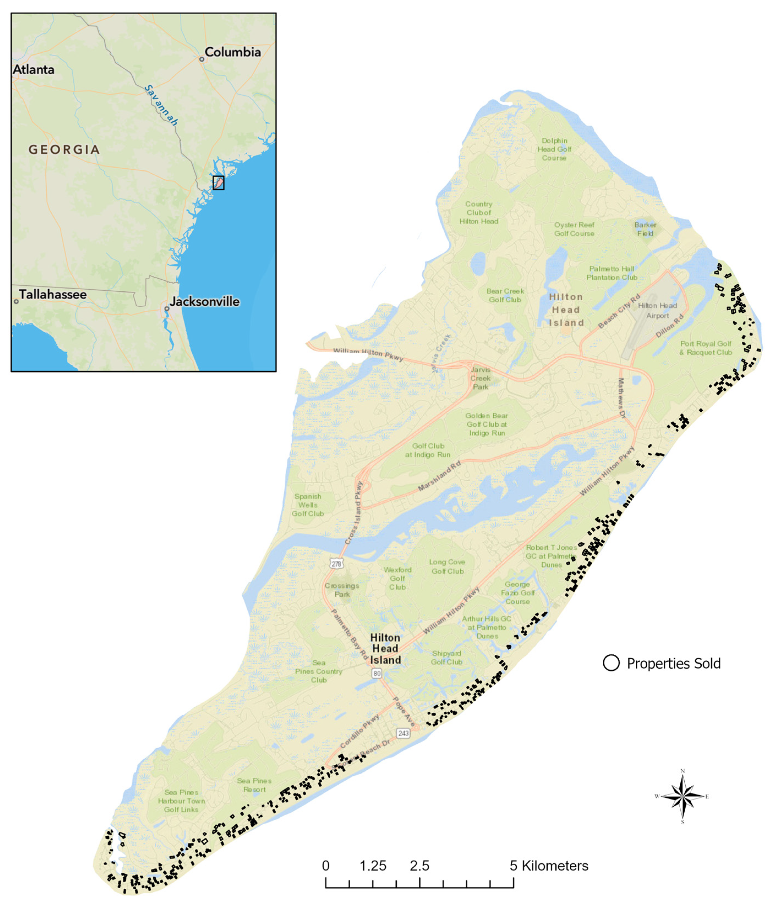
Various data sources were utilized in this study. The condos and single-family houses that were sold between 2011 and 2016 and located within 1500 feet (457 m) of the ocean were included in the analysis. The study area and the properties sold within the 5-year period are presented in Figure 1.
The cut-off distance of 457 m was implemented based on the suggestions by the previous studies [15,19] that examined the impacts of various coastal hazards on property values in similar areas. Landry and Hindsley (2011) [19] examined the impact of negative shoreline change rate on property prices in Tybee Island, GA considering various cut-off distances (100 m to 600 m) from the shoreline. Model parameters for cut-off distances greater than 300 m were found to be statistically insignificant.
Table 1 outlines the variables used in this study along with their sources and descriptions. Variables such as whether the property is a multi-story home, number of bedrooms, presence of garage, number of bathrooms, and size of the living space were included to represent the structural attributes of the properties. While sale prices, year of sale, and location of the properties were obtained from the Beaufort County Assessor’s Office (BCAO), various real estate websites, such as Zillow and Trulia, were utilized to extract structural data. Locational attributes, such as distance from each property to the nearest public beach access point, whether the property is oceanfront or marshfront, and distance to the nearest beach, were estimated using ArcGIS Pro software.
The U.S. Geological Survey (USGS) estimates annual shoreline change rates that can help researchers, government officials, and the general public to identify areas with higher risks of coastal erosion. USGS’s estimates of 30-year change in shoreline positions were used to highlight the areas that experienced negative shoreline changes [21]. Shoreline change rates in meters per year were spatially joined with the property data using ArcGIS Pro. As shown in Table 2, the mean annual shoreline change rate (shrate) in the study area is 0.15 with the values ranging from –1.83 to 5.2. It is important to note that while the positive values indicate accretion, negative values signal eroded beaches. Figure 2 shows the areas of HHI that have been experiencing negative and positive annual shoreline changes.
A dummy variable (shdum) was created to distinguish the areas with erosion and accretion. It was then added to the model to assess the impact of coastal erosion on property values. Additionally, an interaction term (disteros) was created by multiplying the shrate and the distance of each property to the nearest beach (dbeach). Including the distance to the beach variable and shoreline change rates separately within the model may not be enough to obtain the value of shoreline change rate as it is expected that the influence of negative shoreline change rate (shrate) on property values will be different at various distances from the coastline. Relative to households farther from the beach line, oceanfront and other nearby property owners may view eroded beaches more as a means of vulnerability to coastal hazards.
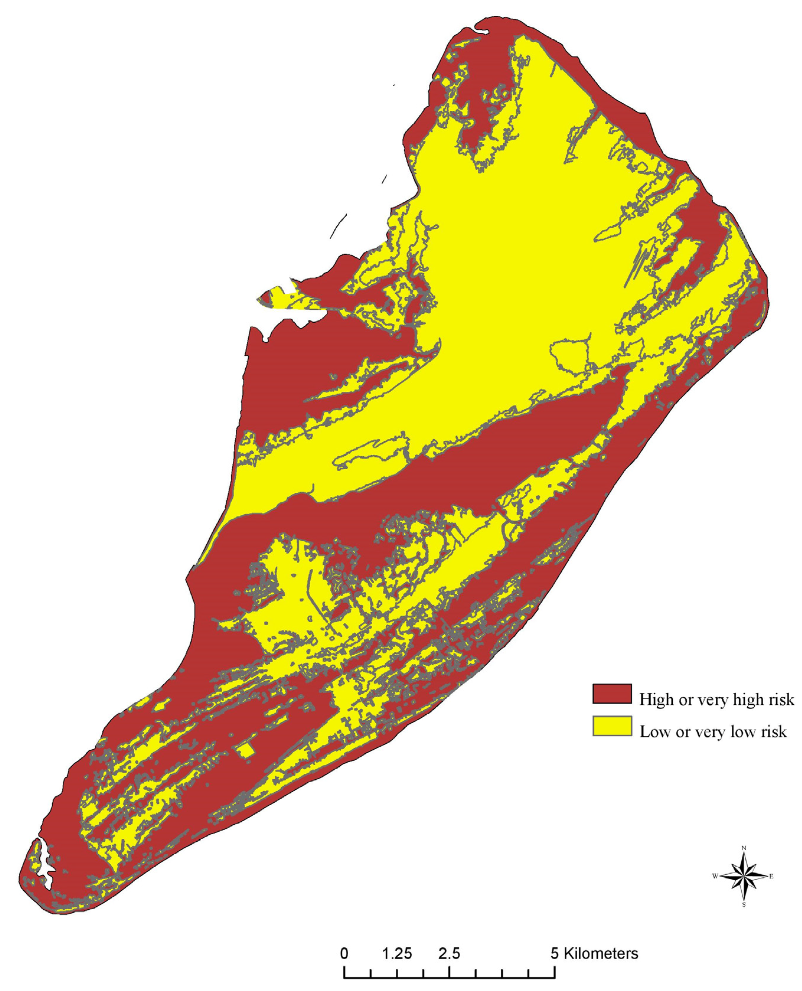
A separate dummy variable (flrisk) was created to incorporate the flood risk into the model. The mean value of flrisk is 0.48, which suggests a balanced mix of risky and non-risky areas in the study area. Flood data is based on the Federal Emergency Management Agency’s (FEMA’s) digital flood insurance rate map, where 1 represents the areas with the least flood risk and 5 represents the most flood risk. Figure 3 shows the areas with high (rating of 4) or very high (rating of 5) and low (rating of 2) or very low (rating of 1) flood risks. It is reasonable to assume that property owners are well informed about the flood risks associated with the properties they purchase, as this information is readily available to them.
4. Method
HPM operates on the assumption that the value of a given property is a function of the following factors:
- The property’s structural attributes, such as lot size, age of home, square footage, etc.
- Locational characteristics, such as distance to coastline, proximity to the closest public or private beach access, etc.
- Environmental attributes, such as shoreline change rate, flood risk, etc.
It is possible to estimate the HPM regression parameters using ordinary least squares (OLS) as long as certain characteristics are met. This parametric model assumes that error terms are normally distributed with zero mean and constant variance. Log-linear function forms have been preferred by the past studies due to nonlinear relationship between home values and independent variables [20,22].
Multicollinearity, an occurrence of strong intercorrelation among predictors, is an assumption of the OLS regression model which can be tested by the variance inflation factor (VIF). The initial model included all the variables listed in Table 2 but the VIF values of dbeach and disteros signalled multicollinearity. Therefore, the distance variable, dbeach, was eliminated from consideration since the interaction term, disteros, has more importance and significance. Additionally, shrate was dropped from consideration due to its collinearity with shdum. The calculated VIF values of the final independent variables ensured a low degree of multicollinearity, as shown in Table 3, where each VIF was found to be less than the threshold of 10 [23].
Checking for the autocorrelation of the errors is an important part of assessing whether a model is well specified. If autocorrelation is detected, the ordinary least squares assumption that the error terms are uncorrelated is violated. The Durbin–Watson statistic, a test to detect the presence of autocorrelation in the residuals from a regression analysis, was conducted, and the score of 1.86 suggests that our dataset has no autocorrelation present. However, working with spatial data requires close attention to spatial autocorrelation among dependent variables and/or error terms, which may also violate OLS assumptions [24].
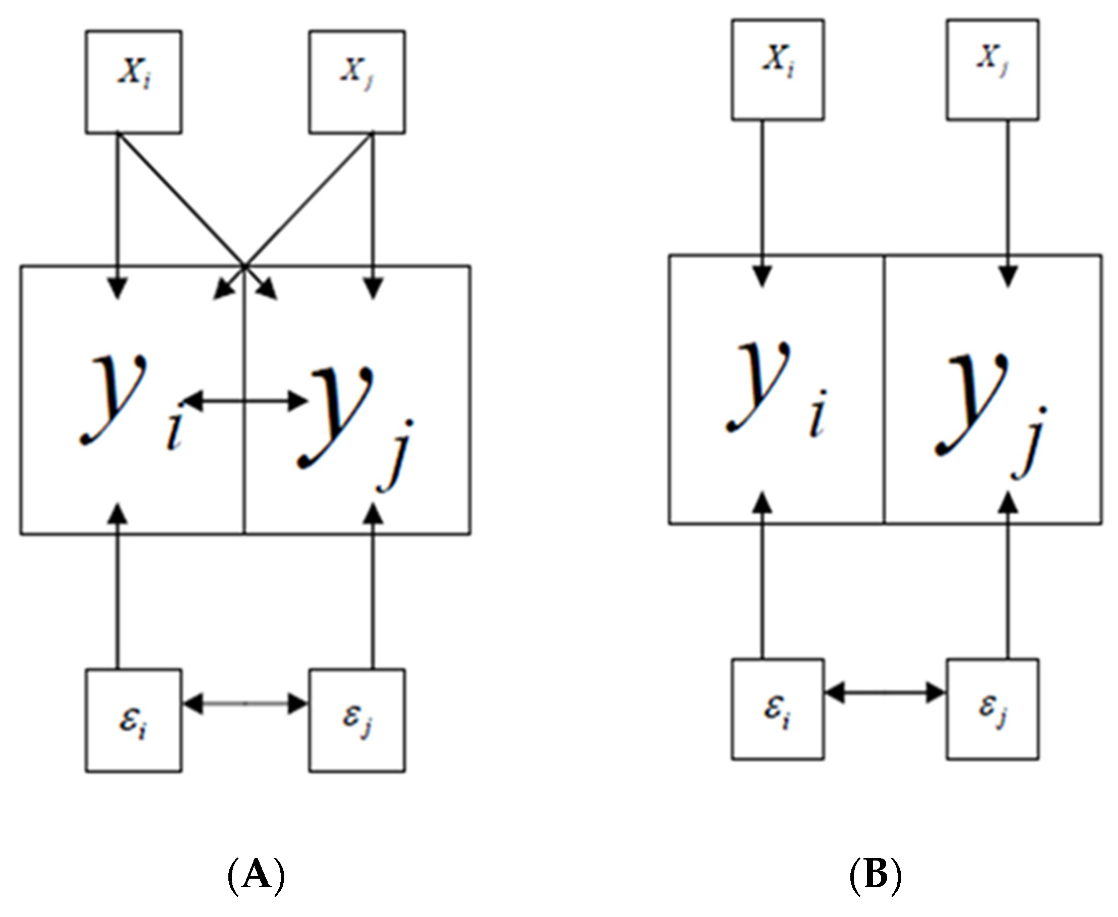
Figure 4A shows the presence of spatial lag dependency where the price of property is not only influenced by its attributes but also the attributes of nearby properties. Error terms of adjacent observations are correlated in Figure 4B. In both cases, OLS assumptions are violated and would lead to biased and inefficient model estimates.
Moran’s I test was conducted to check for general spatial dependency, and the test results are presented in Table 4. A statistically significant value of 0.03 indicates a strong spatial autocorrelation of residuals. Lagrange multiplier for spatial lag and error dependencies tested positive, confirming the presence of both problems in the model. Statistically insignificant robust Lagrange Multiplier (LM) test for spatial error indicated that if spatial dependency is incorporated by adding a spatially lagged dependent variable, the model accuracy would improve. In other words, by including a “spatial” variable as one of the covariates in the model, we can devise a model where home sale value is a function of its attributes and the values of its neighboring properties. This way, the relationship between exogenous variables and the dependent variable can be examined while controlling for spatial dependency in the dependent variable. Therefore, a spatial lag model was adopted to improve the overall accuracy and predictive power of the model.
The endogenous variable is the natural log of the sale price due to nonlinear nature of the data. Using this specification eliminates the heteroscedasticity problem and allows the researchers to interpret a per unit change in each control variable on sale price in percentage terms [25]. After this transformation, the marginal effect for each binary variable should be calculated using (exp(β) − 1) as suggested by Halvorsen and Palmquist (1980) [26]. Year-fixed effects were included to account for any changes that may have occurred over time. A dummy variable for each of the neighbourhoods in the study area was accounted for so locational differences would be controlled.
5. Results and Discussion
OLS, spatial lag, and spatial error models were executed. Since spatial models are based on the estimation of maximum likelihood, reporting and comparing the respective log probabilities is more fitting. Spatial lag model had the highest log-likelihood (−274), confirming the results of the previous tests that accounting for spatial lag dependency would improve model accuracy. Because the spatial error model had slightly lower log-likelihood and produced results that were similar to those of the spatial lag model, Table 5 reports only the results of the OLS (Model 1) and spatial lag (Model 2) regressions. Although there were some minor differences in the magnitude and significance of the regression coefficients among Models 1 and 2, the overall results were quite robust.
The estimates of the parameters are generally statistically significant and have expected signs. The coefficient estimates of dummy variables in parentheses presented in Table 5 are the recalculated coefficients (exp(β) − 1). Spatial variable, introduced to transform the data and remove the dependency among neighbouring dependent variables, is highly statistically significant at 1% level. All structural attributes except the presence of garage have significant impact on property prices. However, garage becomes significant when the spatial variable, spatial, is entered into the regression model (under Model 2) as a separate independent variable. Even though the positive sign of the coefficient of distance to public beach access variable, pbaccess, may seem surprising at first, information about the neighbourhoods in the study area would help us understand this finding. As a property is located away from a public beach access point, the property value is estimated to be increasing, probably because the majority of the properties considered in the study area are located in gated communities with private access to beaches. This finding is consistent with the notion that property owners are likely to pay a premium price (17.9%) for homes that are in gated communities with locational privileges. Because the spatial data for private beach access points was not available, it was not entered into the model as a separate exogenous variable.
For an average home in the study area, an additional bedroom and bathroom are expected to increase the value of the property by approximately $76 K and $213 K, respectively (average home price is $1,354,000 in the study area). The presence of a garage, based on spatial lag model results, account for 8.1% of the value of the property. Single-family homeowners are expected to pay a 17.6 percent premium because single-family homes have more valuable features than condominiums. As the size of the living space in a property increases by 1 square foot, property value is expected to increase by 0.00004% which is the equivalent of $54 for an average home in the study area. Model (2) findings also show that for waterfront properties that are either oceanfront or marshfront, buyers pay a substantial price premium (96 percent). This finding is consistent with the past studies which produced evidence that having water views would enhance property values [12,15].
The coefficient of flrisk has the expected sign and is statistically significant at 1% level. The presence of high or very high flood risk lowers property values by 15.6%. The price discount is consistent with the previous studies [15,16,27] that flood risk would reduce property values. Flood zone designations that are available to potential property owners provide information about the flood risk that seem to affect buyer behaviours and price decisions.
The coefficient of shdum is highly statistically significant with an estimated value of –0.26. This finding confirms that shoreline erosion risk is capitalized into residential property prices. Being located within an area with negative shoreline change rate lowers the property value by approximately 26% in the study area. Additionally, the interaction term, disteros, is also statistically significant at 1% level. A statistically significant interaction term with negative sign indicates that risk of shoreline erosion is capitalized less into property values as a property is located further away from the coastline. A distance of 214 m was determined to be the cut-off distance after accounting for this diminishing impact. In other words, for the homes that are located over 214 m from the beach line, the marginal value of additional change in the shoreline change rate is zero. This may be partially because properties that are situated further from the shoreline have access to the larger protective buffer.
6. Discussion and Conclusions
Climate change is one of the Earth’s greatest environmental challenges. Elevated risks of coastal hazards due to rising average temperatures have been causing damages to infrastructure and loss of ecosystems for years. Similar to other coastal cities and towns, HHI, South Carolina’s largest barrier island, has been facing this challenge. Half of the properties that are in close proximity to the coastline are in areas with high or very high flood risk. Moreover, a significant portion of the HHI beaches has been eroded at a faster pace due to sea-level rise.
In this paper, the HPM was implemented to check whether the risks of flooding and beach erosion were capitalized into residential real estate prices. Spatial autocorrelation tests were performed to check for any form of spatial dependency that could be present in the dataset so the right model specification would be chosen to improve model accuracy. Spatial lag specification was adopted to account for spatial dependency among the neighboring properties. The results of the OLS and spatial error models were not significantly different than those of the spatial lag model, but they produced slightly lower statistical accuracy.
The results of the spatial lag model show that flood risk is an important deciding factor when potential homeowners are actively searching for residential properties. Properties that are in flood zones are discounted by about 15.6%. This is consistent with the notion that buyers who pay high insurance premiums for flood risk-prone properties pay lower prices at the time of sale [28]. For a more comprehensive analysis, it may be worthwhile to extend the study area by including all the properties on the island, regardless of their proximity to shoreline.
The findings of this study show that the relationship between beach erosion and property values is significant in HHI. The negative shoreline change rate, as an indicator of beach erosion, is observed to reduce the property values that are located within 214 m of the beach line. Homeowners’ willingness to pay for lower erosion is higher when a property is located closer to the beach. This effect declines and eventually disappears as property is located further away from the ocean. It is important to note that future studies should focus on capturing the perceptions of property owners about erosion risks so that more realistic willingness to pay estimates can be captured.
Capitalization of erosion risk is an important first step to produce an accurate cost-benefit analysis of best management practices to combat this problem. Hard stabilization and beach nourishment projects are some of the practices that provide not only recreational benefits to the residents and the property owners but also protection to the nearby properties serving as buffers from beach erosion. It is critical to know the true cost of coastal erosion or benefit of reducing its risk so optimal policy strategies and programs can be implemented. For example, the burden of a potential tax program to finance an adaptive strategy to lower beach erosion risk can be allocated based on the quantification of the benefits taxpayers would receive in exchange. The property owners who own oceanfront or nearby properties could pay more in taxes to finance a stabilization program that would lower the risk of property damage. Such policy would ensure that those who benefit the most from owning a property in a coastal location also endure the associated risks of shoreline change.
Funding
This research received no external funding.
Informed Consent Statement
Not applicable.
Data Availability Statement
Publicly available datasets were analyzed in this study. This data can be found here: https://www.beaufortcountytreasurer.com/, accessed on 3 August 2020.
Conflicts of Interest
The author declares that there are no conflict of interest.
References
- Carey, T.R.; Salazar, J. Estimated Total Impact of Tourism in Hilton Head Island, 2019 on Beaufort County, South Carolina; Regional Transactions Concepts, LLC: Pendleton, SC, USA, 2020; Available online: http://www.thinkhiltonheadisland.org/article-details?hhaid=736 (accessed on 2 February 2020).
- Bretz, L. Climate Change and Homes: Who Would Lose the Most to a Rising Tide? 2017. Available online: https://www.zillow.com/research/climate-change-underwater-homes-2-16928/ (accessed on 1 May 2020).
- Syvitski, J.P.M.; Kettner, A.J.; Overeem, I.; Hutton, E.W.H.; Hannon, M.T.; Brakenridge, G.R.; Day, J.W.; Vorosmarty, C.J.; Saito, Y.; Giosan, L.; et al. Sinking deltas due to human activities. Nat. Geosci. 2009, 2, 681–686. [Google Scholar] [CrossRef]
- Hoyos, C.D.; Agudelo, P.A.; Webster, P.J.; Curry, J.A. Deconvolution of the Factors Contributing to the Increase in Global Hurricane Intensity. Science 2006, 312, 94–97. [Google Scholar] [CrossRef] [PubMed] [Green Version]
- Emanuel, K. Assessing the present and future probability of Hurricane Harvey’s rainfall. Proc. Natl. Acad. Sci. USA 2017, 114, 12681–12684. [Google Scholar] [CrossRef] [PubMed] [Green Version]
- Wdowinski, S.; Bray, R.; Kirtman, B.P.; Wu, Z. Increasing flooding hazard in coastal communities due to rising sea level: Case study of Miami Beach, Florida. Ocean Coast. Manag. 2016, 126, 1–8. [Google Scholar] [CrossRef]
- McAlpine, S.A.; Porter, J.R. Estimating Recent Local Impacts of Sea-Level Rise on Current Real-Estate Losses: A Housing Market Case Study in Miami-Dade, Florida. Popul. Res. Policy Rev. 2018, 37, 871–895. [Google Scholar] [CrossRef] [PubMed] [Green Version]
- Kulp, S.A.; Strauss, B.H. New elevation data triple estimates of global vulnerability to sea-level rise and coastal flooding. Nat. Commun. 2019, 10, 1–12. [Google Scholar] [CrossRef] [Green Version]
- Vousdoukas, M.I.; Ranasinghe, R.; Mentaschi, L.; Plomaritis, T.A.; Athanasiou, P.; Luijendijk, A.; Feyen, L. Sandy coastlines under threat of erosion. Nat. Clim. Chang. 2020, 10, 260–263. [Google Scholar] [CrossRef]
- Landry, C.E.; Keeler, A.G.; Kriesel, W. An Economic Evaluation of Beach Erosion Management Alternatives. Mar. Resour. Econ. 2003, 18, 105–127. [Google Scholar] [CrossRef]
- Samarasinghe, O.; Sharp, B. Flood prone risk and amenity values: A spatial hedonic analysis. Aust. J. Agric. Resour. Econ. 2010, 54, 457–475. [Google Scholar] [CrossRef] [Green Version]
- Below, S.; Eli, B.; Hilla, S. Land Erosion and Coastal Home Values. J. Real Estate Res. 2015, 37, 499–535. [Google Scholar]
- Kriesel, W.; Lichtkoppler, F.; Randall, A. Estimating the benefits of shore erosion protection in Ohio’s Lake Erie Housing Market. Water Resour. Res. 1993, 29, 795–801. [Google Scholar] [CrossRef]
- Atreya, A.; Czajkowski, J. Housing Price Response to the Interaction of Positive Coastal Amenities and Negative Flood Risks (Working Paper No. 2014-09). 2014. Available online: https://pdfs.semanticscholar.org/ffd4/547e241e346df6023820aa0f9cd7e8694caa.pdf (accessed on 1 March 2020).
- Bin, O.; Crawford, T.W.; Kruse, J.B.; Landry, C.E. Viewscapes and Flood Hazard: Coastal Housing Market Response to Amenities and Risk. Land Econ. 2008, 84, 434–448. [Google Scholar] [CrossRef]
- Turnbull, G.K.; Zahirovic-Herbert, V.; Mothorpe, C. Flooding and Liquidity on the Bayou: The Capitalization of Flood Risk into House Value and Ease-of-Sale. Real Estate Econ. 2012, 41, 103–129. [Google Scholar] [CrossRef]
- Bin, O.; Kruse, J.B.; Landry, C. Flood Hazards, Insurance Rates, and Amenities: Evidence from the Coastal Housing Market. J. Risk Insur. Am. Risk Insur. Assoc. 2018, 75, 63–82. [Google Scholar] [CrossRef]
- Roberts, R.; Beckley, L.E.; Tull, M. The Economic Value of Cyclonic Storm-Surge Risks: A Hedonic Case Study of Residential Property in Exmouth, Western Australia. In Climate Change in the Asia-Pacific Region. Climate Change Management; Leal Filho, W., Ed.; Springer: Cham, Switzerland, 2015. [Google Scholar]
- Landry, C.E.; Hindsley, P. Valuing Beach Quality with Hedonic Property Models. SSRN Electron. J. 2011. [Google Scholar] [CrossRef]
- Jin, D.; Hoagland, P.; Au, D.K.; Qiu, J. Shoreline change, seawalls, and coastal property values. Ocean Coast. Manag. 2015, 114, 185–193. [Google Scholar] [CrossRef]
- Kratzmann, M.G.; Himmelstoss, E.A.; Thieler, E.R. National Assessment of Shoreline Change—A GIS Compilation of Updated Vector Shorelines and Associated Shoreline Change Data for the Southeast Atlantic Coast; U.S. Geological Survey Data Release; U.S. Geological Survey: Reston, VA, USA, 2017. [CrossRef]
- Gopalakrishnan, S.; Smith, M.D.; Slott, J.M.; Murray, A.B. The Value of Disappearing Beaches: A Hedonic Pricing Model with Endogenous Beach Width. J. Environ. Econ. Manag. 2011, 61, 297–310. [Google Scholar] [CrossRef] [Green Version]
- Lin, F.J. Solving Multicollinearity in the Process of Fitting Regression Model Using the Nested Estimate Proce-dure. Qual. Quant. Int. J. Methodol. 2008, 42, 417–426. [Google Scholar] [CrossRef]
- Chasco, C.; Gallo, J.L. Hierarchy and Spatial Autocorrelation Effects in Hedonic Models. Econ. Bull. 2012, 32, 1474–1480. [Google Scholar]
- Sirmans, G.S.; Macpherson, D.A.; Zietz, E.N. The Composition of Hedonic Pricing Models. J. Real Estate Lit. 2005, 13, 3–43. [Google Scholar]
- Halvorsen, R.; Palmquist, R. The Interpretation of Dummy Variables in Semilogarithmic Equations. Am. Econ. Rev. Am. Econ. Assoc. 1980, 70, 474–475. [Google Scholar]
- Shultz, S.; Fridgen, P.M. Floodplains and housing values: Implications for flood mitigation projects 1. JAWRA J. Am. Water Resour. Assoc. 2001, 37, 595–603. [Google Scholar] [CrossRef]
- Troy, A.R.; Romm, J. Assessing the price effects of flood hazard disclosure under the California natural hazard disclosure law (AB 1195). J. Environ. Plan. Manag. 2004, 47, 137–162. [Google Scholar] [CrossRef]
Figure 1.
Location of the study area and the properties sold.

Figure 2.
Annual shoreline change rates.
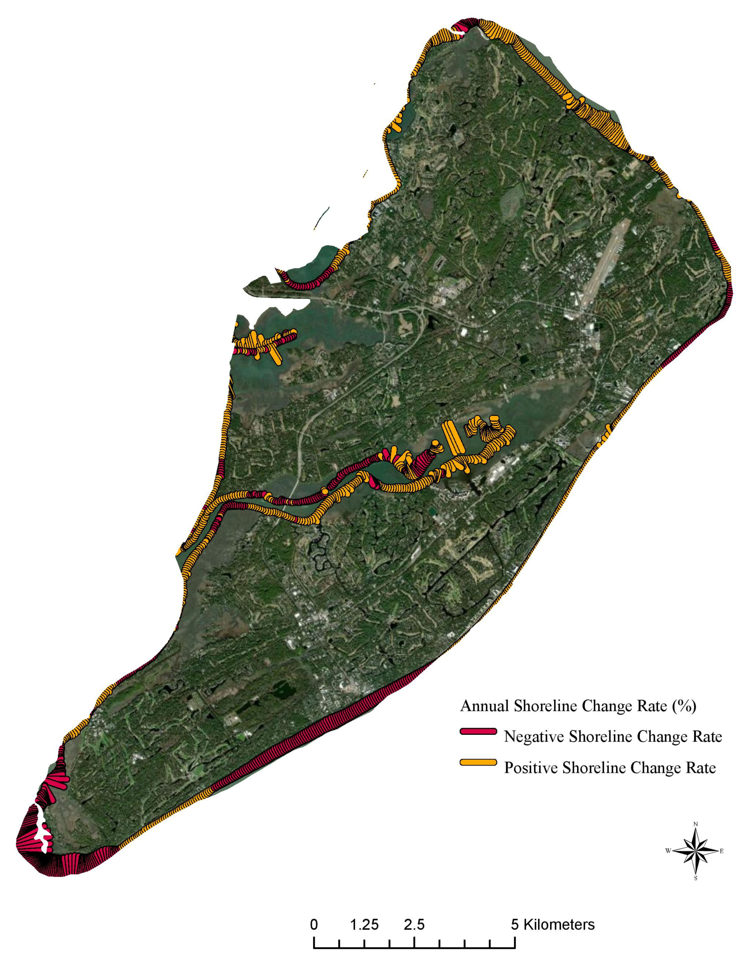
Figure 3.
Flood risk map.

Figure 4.
Spatial dependency ((A)—spatial lag dependency; (B)—spatial error dependency).


Table 1.
Variable descriptions and data sources.
| Variable | Description | Source |
|---|---|---|
| singfam | 1 if property is a single-family home; 0 otherwise | Beaufort County Assessor’s Office (BCAO) |
| pbaccess | Distance to nearest public beach access point (meters) | ArcGIS Pro |
| footage | Size of the living space in the property (square feet) | BCAO |
| numbed | Number of bedrooms | Zillow |
| numbath | Number of bathrooms | Zillow |
| garage | 1 if property has garage space; 0 otherwise | Zillow |
| mstory | 1 if property is single-storied; 0 otherwise | Zillow |
| gated | 1 if property is located in a gated community; 0 otherwise | Zillow |
| waterfr | 1 if property is oceanfront or marshfront; 0 otherwise | ArcGIS Pro |
| shrate | Change in shoreline position (in meters) per year. | USGS [12] |
| shdum | 1 if annual change in shoreline position is negative; 0 if positive. | USGS [12] |
| dbeach | Distance to the nearest beach (in meters) | ArcGIS Pro |
| disteros | shrate*dbeach (in square meter) | ArcGIS Pro |
| flrisk | 1 if the property is located where flood risk is high or very high; 0 if the flood risk is low or very low. | Federal Emergency Management Agency (FEMA) |
| year | Year of sale, 1 (2011) to 6 (2016) | BCAO |
Table 2.
Descriptive statistics of the sale prices of the homes sold in the study area and their structural, locational, and environmental attributes.
Table 2.
Descriptive statistics of the sale prices of the homes sold in the study area and their structural, locational, and environmental attributes.
| Variable | Mean | Std. Dev. | Minimum | Maximum |
|---|---|---|---|---|
| sale price (000s)($) | 1354 | 1141 | 69.5 | 7270 |
| Singfam | 0.92 | 0.27 | 0 | 1 |
| pbaccess (meters) | 749 | 402 | 12 | 1940 |
| footage (square feet) | 3562 | 1763 | 1118 | 13,060 |
| numbed | 4.23 | 1.30 | 1 | 8 |
| numbath | 4.34 | 1.70 | 1 | 9 |
| garage | 0.70 | 0.46 | 038 | 1 |
| mstory | 0.62 | 0.49 | 0 | 1 |
| gated | 0.73 | 0.45 | 0 | 1 |
| waterfr | 0.22 | 0.42 | 0 | 1 |
| shrate (meters per year) | 0.15 | 1.46 | −1.83 | 5.23 |
| shdum | 0.44 | 0.49 | 0 | 1 |
| dbeach (meters) | 211 | 125 | 5 | 456 |
| Disteros (square meters) | 228 | 344 | −327 | 3381 |
| flrisk | 0.48 | 0.50 | 0 | 1 |
| year | 3.39 | 1.59 | 1 | 6 |
Table 3.
Multicollinearity test results.
| Variable | Variance Inflation Factors (VIF) |
|---|---|
| singfam | 1.27 |
| pbaccess | 1.55 |
| footage | 1.56 |
| numbed | 2.40 |
| numbath | 3.02 |
| garage | 1.25 |
| mstory | 1.40 |
| gated | 1.78 |
| waterfr | 1.29 |
| shdum | 1.12 |
| disteros | 1.25 |
| flrisk | 1.12 |
Table 4.
Detection of spatial autocorrelation.
| Test | Value | Probability |
|---|---|---|
| Moran’s I (error) | 0.13 | 0.01263 |
| Lagrange Multiplier (lag) | 11.02 | 0.00090 |
| Robust LM (lag) | 7.47 | 0.00627 |
| Lagrange Multiplier (error) | 3.76 | 0.05200 |
| Robust LM (error) | 0.2237 | 0.00361 |
Table 5.
Regression results.
| OLS (Model 1) | Spatial Lag (Model 2) | |||
|---|---|---|---|---|
| Variable | Parameter | Standard Error | Parameter | Standard Error |
| spatial | - | - | 0.26642 *** | 0.07606 |
| singfam | 0.16516 ** (0.17958) | 0.08162 | 0.16180 ** (0.1756) | 0.07912 |
| Pbaccess (meters) | 0.00004 *** | 0.00001 | 0.00003 *** | 0.00001 |
| Footage (square feet) | 0.00004 *** | 0.00001 | 0.00004 *** | 0.00001 |
| numbed | 0.05296 ** (0.05438) | 0.02322 | 0.05448 ** (0.05599) | 0.02250 |
| numbath | 0.15054 *** (0.16246) | 0.01998 | 0.14595 *** (0.1571) | 0.01938 |
| garage | 0.07195 (0.0746) | 0.04751 | 0.07792 * (0.0810) | 0.04603 |
| mstory | −0.09457 ** (−0.09024) | 0.03777 | −0.09489 *** (−0.09053) | 0.0366 |
| gated | 0.20917 *** (0.23265) | 0.05844 | 0.16478 *** (0.17913) | 0.05731 |
| waterfr | 0.64862 *** (0.9128) | 0.67407 | 0.67407 *** (0.9622) | 0.05147 |
| shdum | −0.35015 *** (−0.2954) | 0.08787 | −0.30116 *** (−0.26004) | 0.08579 |
| Disteros (square meters) | −0.00027 *** | 0.00006 | −0.00025 *** | 0.00006 |
| flrisk | −0.15888 *** (−0.1469) | 0.04126 | −0.17007 *** (−0.1563) | 0.04015 |
| location effects | yes | yes | ||
| year fixed effects | yes | yes | ||
| In L | −280 | −274 | ||
| R2 | 0.605 | 0.628 | ||
| Observations | 495 | 495 | ||
*** p < 0.01, ** p < 0.05, * p < 0.10.
Publisher’s Note: MDPI stays neutral with regard to jurisdictional claims in published maps and institutional affiliations. |
© 2021 by the author. Licensee MDPI, Basel, Switzerland. This article is an open access article distributed under the terms and conditions of the Creative Commons Attribution (CC BY) license (http://creativecommons.org/licenses/by/4.0/).
Share and Cite
MDPI and ACS Style
Catma, S. The Price of Coastal Erosion and Flood Risk: A Hedonic Pricing Approach. Oceans 2021, 2, 149-161. https://0-doi-org.brum.beds.ac.uk/10.3390/oceans2010009
AMA Style
Catma S. The Price of Coastal Erosion and Flood Risk: A Hedonic Pricing Approach. Oceans. 2021; 2(1):149-161. https://0-doi-org.brum.beds.ac.uk/10.3390/oceans2010009
Chicago/Turabian StyleCatma, Serkan. 2021. "The Price of Coastal Erosion and Flood Risk: A Hedonic Pricing Approach" Oceans 2, no. 1: 149-161. https://0-doi-org.brum.beds.ac.uk/10.3390/oceans2010009