
Optimal Life Extension Management of Offshore Wind Farms Based on the Modern Portfolio Theory


Centre for Marine Technology and Ocean Engineering (CENTEC), Instituto Superior Técnico, University of Lisbon, 1049-001 Lisbon, Portugal
*
Author to whom correspondence should be addressed.
Oceans 2021, 2(3), 566-582; https://0-doi-org.brum.beds.ac.uk/10.3390/oceans2030032
Submission received: 26 May 2021
/
Revised: 13 August 2021
/
Accepted: 18 August 2021
/
Published: 24 August 2021
(This article belongs to the Special Issue Sustainable Marine Structures)
Abstract
:The present study aims to develop a risk-based approach to finding optimal solutions for life extension management for offshore wind farms based on Markowitz’s modern portfolio theory, adapted from finance. The developed risk-based approach assumes that the offshore wind turbines (OWT) can be considered as cash-producing tangible assets providing a positive return from the initial investment (capital) with a given risk attaining the targeted (expected) return. In this regard, the present study performs a techno-economic life extension analysis within the scope of the multi-objective optimisation problem. The first objective is to maximise the return from the overall wind assets and the second objective is to minimise the risk associated with obtaining the return. In formulating the multi-dimensional optimisation problem, the life extension assessment considers the results of a detailed structural integrity analysis, a free-cash-flow analysis, the probability of project failure, and local and global economic constraints. Further, the risk is identified as the variance from the expected mean of return on investment. The risk–return diagram is utilised to classify the OWTs of different classes using an unsupervised machine learning algorithm. The optimal portfolios for the various required rates of return are recommended for different stages of life extension.
1. Introduction
Offshore wind turbine (OWT) structures approaching the end of their service lives are in a structural condition for extended use, mainly due to the conservative design philosophies and operation policies adopted by the oil and gas offshore industry. In this regard, the offshore wind industry is searching for a reliable guideline for certification assuring a structural capacity above the permissible limit within the desired extended service life at minimal operational cost. Such policies can only be achieved by comprehensive life extension assessment that encapsulates both technical and economic analysis. The techno-economic analyses for life-cycle extension projects must incorporate structural health monitoring data, detailed structural integrity assessment, condition-based maintenance and detailed financial analysis. Furthermore, developing a guideline that helps the life extension certification requires a multi-disciplinary approach involving state-of-the-art modelling, analysis and prediction techniques using the experience gained from the research centred on design and life-cycle optimisation of OWTs.
To tackle the challenges mentioned above and which contribute to the current state of the art, the present work aims to develop a novel approach to finding optimal solutions for life extension management for a multi-unit offshore wind farm based on Markowitz’s modern portfolio theory, adapted from finance. This novel approach is developed based on the assumption that offshore wind turbines can be considered a cash-producing tangible asset that provides a positive return from the initial investment with a given risk attaining the targeted return. In this regard, the present study performs a techno-economic life extension analysis within the scope of the multi-objective optimisation problem. The first objective is to maximise the return from the overall wind assets, while the latter aims to minimise the risk associated with obtaining the return.
The modern portfolio theory, MPT, was created by Markowitz [1] based on the premise that investors are risk-averse. They aim to maximise the expected return from the selection of the possible investment options. MPT pioneered the quantitative financial analysis by suggesting the investment selection is a quadratic optimisation problem with linear constraints to maximise the overall return and minimise the risk [2].
This multi-objective optimisation problem resulted in the construction of an efficient frontier [3]. The MPT was later modified by Sharpe [4] and Treynor [5,6] to build a generalised theory for the capital asset pricing model to assist investment decision-making. The modern portfolio theory and capital asset pricing model provided a decent way of looking at the equilibrium between risky assets with a different expected return and a tool for measuring the performance of available investment strategies.
The modern portfolio theory is built on many assumptions. However, one assumption draws more reaction than the others is that risk can be measured as the dispersion of dataset of returns relative to its mean value, in other words, standard deviation. Maier-Paape and Zhu [7,8] reviewed the definition of the risk within the context of modern portfolio theory, its limitations, objections and some alternative risk measures.
The importance of risk in offshore wind projects and of risk mitigation by diversification has been addressed in earlier studies. In this regard, Green and Vasilakos [9] suggested that it might prove economic to build an international offshore grid connecting wind farms belonging to different countries situated close to each other. Levitt et al. [10] highlighted that these risk policies and finance structures also have a strong influence on wind power prices, and that wind prices are justifiably scattered depending on the riskiness of the project as they are categorised from high to low risk as first of a kind, global average, and best recent values. Further, Blanco [11] stated that de-regularisation of the power market would lead to risk exposure to the profitability of the investment. The studies mentioned above identified some critical elements for financing and managing the life cycle that need to be accounted for in the multi-disciplinary risk-based life extension analysis.
Although Markowitz’s modern portfolio theory was initially developed for financial assets, there has been quite an interest in applying the theory for non-financial assets because it allows for an overall assessment of portfolios consisting of asset groups of different risk levels instead of analysing each portfolio asset individually. Further, it allows for a minimisation of risk through diversification, which is one of the main premises of the MPT.
Chaves-Schwinteck [12] provided comprehensive research on the applicability of modern portfolio theory to wind farm investments. The study was based on a critical review of the already published works that mainly focused on risk mitigation through geographical diversification (different wind farm locations) [13,14] and renewable energy asset diversification (a portfolio of solar, wind and hydro) [15]. Chaves-Schwinteck [12] underlined the difference in the definition of risk between a long-term infrastructure project and a short-term financial investment. However, the research also acknowledged that using appropriate diversification MPT can be a good tool for risk mitigation strategy for wind farm investment by optimising the wind regime and technical risk details of the operation of a wind farm. Besides, a number of studies have attempted the application of the modern portfolio theory to take advantage of the power of diversification to mitigate the overall project risk and optimise the portfolio of energy production assets [15,16,17,18,19,20,21,22].
In terms of the offshore wind industry, Cunha and Ferreira [22] presented a study in which diversification can help reduce the variability in energy production, which aimed to assist the decision-making process related to the geographic location of offshore wind investments. Thomaidis et al. [23] also stated the advantages of power mixes compared to single-site installation. The result of the study highlighted the benefits of diversification by showing that the sites with high variability (risky assets) could add value to the portfolio. In addition, Schmidt et al. [24] contributed to arguments for diversification of offshore wind assets since a premium feed-in tariff scheme incentivised the spatial diversification. Delarue et al. [25] accounted for the variability of wind power in a portfolio theory model, aiming to distinguish between installed energy, electricity generation and actual instantaneous power. Further, deLlano-Paz et al. [26] gave an exhaustive review of the literature concerning the application of MPT to the field of energy planning and electricity production, explaining the limits to the MPT and to the concept of risk as well as adjustability to the reality of the electricity market alongside its contribution from the financial and energy standpoint.
The present study aimed to contribute to the literature by developing a risk-based approach to deal with the life extension management of offshore wind assets. Markowitz’s MPT obtains the optimal operational management strategy for targeted returns with minimal risk. To achieve this goal, firstly, a techno-economic life extension analysis was conducted to attain the mean value of return and variance from the mean value, which is denoted as risk. Afterwards, the resulting risk−return diagram was used to classify the offshore wind assets using unsupervised machine learning, k-means clustering algorithm. The appropriate weighting factor was estimated for a set of different offshore wind assets through an optimisation process that minimised the risk for a targeted mean of return. The study cases were generated for different stages of the life extension to give recommendations regarding how to navigate during a life extension with the efficient portfolios of offshore wind turbines.
2. Modern Portfolio Theory (MPT) and Portfolio Optimisation
Markowitz’s MPT acknowledges the trade-off between the expected return and corresponding risk. The theory argues that the expected return should be evaluated by an investor concerning the risk an investor is willing to take to earn the expected return. Within this context, MPT helps to build multiple assets that maximise the expected returns for a given level of risk or minimise the risk for a given level of return.
The modern portfolio theory heavily relies on statistical time-series measures (moments). These statistical measures are mean value, standard deviation, covariance, cross-correlation and auto-correlation. The mean value denotes the performance (arithmetic mean for expected, geometric mean for achieved performance) and the standard deviation denotes the riskiness of the asset. The covariance indicates the systematic risk, which cannot be removed by diversifying the overall risk in the portfolio of assets. The cross-correlation denotes how two given assets move together, and the auto-correlation represents the informational efficiency of the asset that shows how it moves in time. The present study performs portfolio optimisation for life extension management based on the first four measures, assuming that the autocorrelation of all assets is zero, meaning that return on investment would reflect all the information without any time lag.
The correlation between the assets is as significant as the mean value and standard deviation because it defines to what extend the risk can be minimised within a diversified portfolio. When the correlation between the two assets is −1, the total risk of the portfolio of those two assets becomes minimum, whereas when two assets are fully correlated, correlation is 1, the entire risk or standard deviation of the portfolio becomes the weighted sum of the standard deviations of those two assets.
The effect of the correlation on the success of the risk mitigation via diversification becomes more relevant for life extension of offshore wind turbines than the beginning of the life-cycle because the offshore wind assets are expected to be less correlated with each other over the service life.
Following the description given above, Markowitz’s portfolio theory can be expressed as follows:
where µp is the mean value of returns of the portfolio, wi is the weighting factor related to each asset and µi is the mean value of returns of each asset. The variance of returns is expressed as follows:
where σp is the standard deviation of return of the portfolio, which indicates the level of risk of the overall portfolio and σij is the covariance between two assets which is calculated as:
where ρij is the correlation between the two assets. For a large number of assets, the standard deviation of return of the portfolio is as follows:
As the correlation approximates 1, the portfolio’s standard deviation approximates the weighted product of the standard deviation of return of each asset, which means that the portfolio selection does not reduce the risk caused by individual assets.
In essence, the modern portfolio theory constitutes a multi-objective (maximum return, minimum risk) optimisation problem that leads to an efficient frontier. The efficient frontier is built similar to the Pareto optimality front (frontier), which accepts the riskier asset as long as the asset’s mean value is higher, or, accepts a lower return as long as the asset is less risky. It is worth mentioning that the efficient frontier tends to be nonlinear, showing behaviours such as diminishing marginal return to risk. This means that it requires more risk-taking to get a unit increment of the expected return.
Another underlying assumption of the modern portfolio theory is that the asset return follows a normal distribution, which might not represent the reality as the distribution of the asset returns can be fat-tailed distribution and might have a tail and asymmetric dependence and can show non-stationary (time-varying) time-series attributes. In failing to comply with these normality assumptions, the investor is subjected to heavy downside risk, and a risk-averse investor is intolerant to downside risk.
The critics of the modern portfolio theory suggest that there are significant flaws regarding the underlying assumptions, such as normality assumptions, returns reflecting complete information, and risk definition assumptions. To address these assumptions, post-modern portfolio theory was introduced, focusing on the downside risk of returns. The suspicious take on the modern portfolio theory and its place in the investment world has its merit; nevertheless, the application of the modern portfolio theory to offshore wind asset managements is still quite an interesting research topic as the underlying assumptions regarding the return, volatility and correlation can be obtained through a number of statistical analyses and confirmed before the use of the MPT, which is essentially the case for the present work.
The line drawn from the risk-free asset rf tangent to the efficient frontier is called the optimised risk/return relationship (Sharpe ratio) along the efficient frontier. The most efficient portfolio is identified as the highest Sharpe ratio. An investor who does not define a preference function (utility function), which is a function of risk-averseness, should accept the portfolio with the highest Sharpe ratio.
The optimised portfolio with the highest Sharpe ratio is a concept that can be utilised for the diversified offshore wind asset portfolio. Nevertheless, it is also possible to attain efficient portfolios as a function of the risk-averseness of the decision-makers. One can be advised to accept more risk-tolerant preference at the beginning of the life extension. The level of risk-averseness could be increased towards the end of the life extension, and this is precisely the research question that was undertaken in the present work.
3. Life Extension Assessment and Offshore Wind Asset Classification
The prerequisite of the modern portfolio selection is to have the first two moments of the sample offshore wind farm data, the mean value and standard deviation. The mean value denotes the expected return, and the standard deviation indicates the risk associated with the asset. To this end, a comprehensive life-cycle assessment covering both technical and economic aspects is conducted in a Monte Carlo simulation. The techno-economic life-cycle assessment results are used to classify different offshore wind assets based on a risk−return diagram.
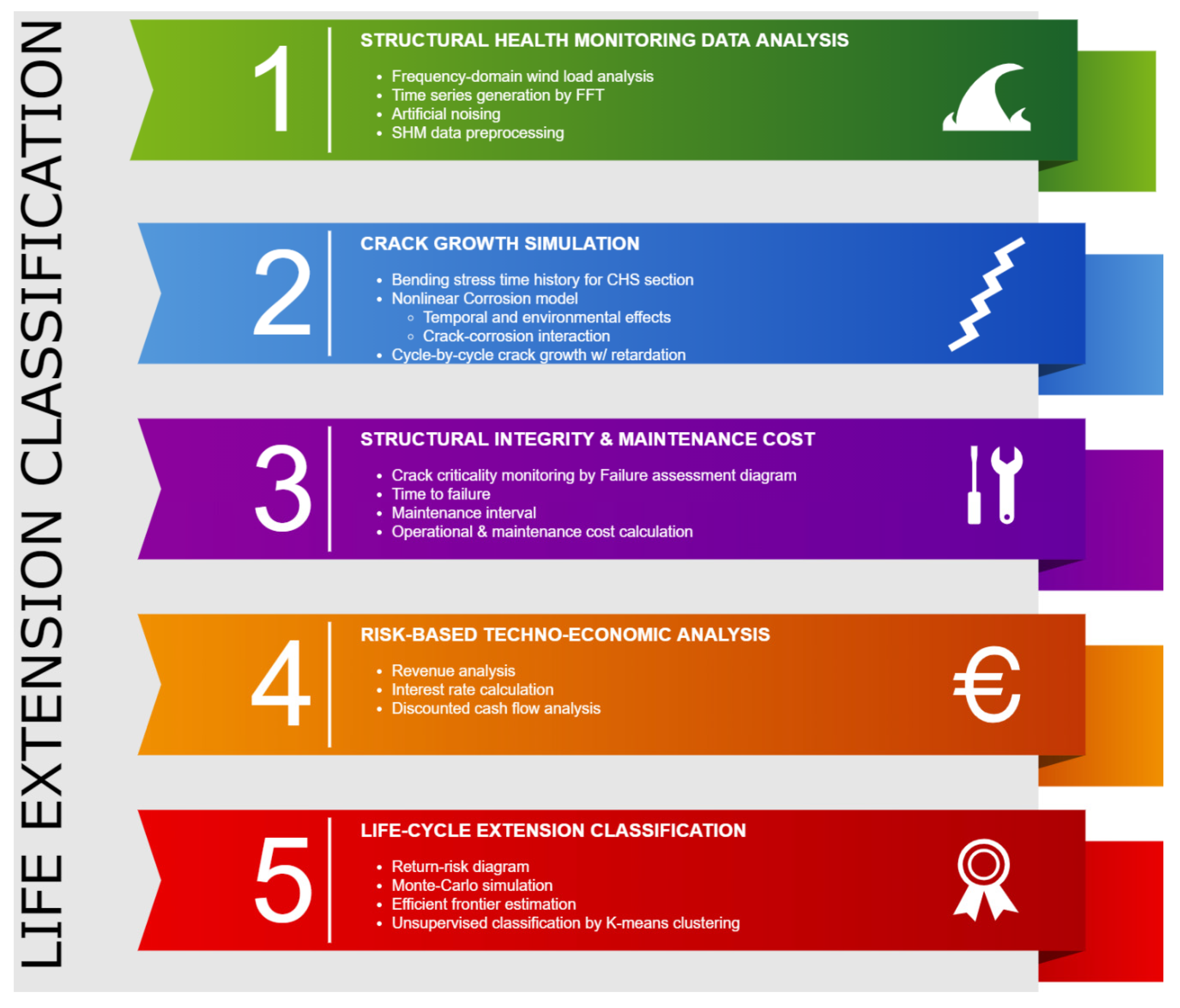
The methodology used for the classification consists of five stages, as seen in Figure 1. The procedure commences with preprocessing data collected by the structural health monitoring system, followed by a corrosion-induced crack growth simulation and structural integrity analysis to estimate the maintenance interval and overall operational costs.
The structural health monitoring system processes the SCADA system’s wind-induced load data. It removes the noise from the signal using the low-pass filter (frequency domain) or Gaussian running-mean filter (time domain). The preprocessed time signal is then analysed to obtain the wind-induced bending stress at the transition piece, where corrosion affects the support structure the most. The corrosion-induced crack growth simulation is conducted based on fracture mechanics in the time domain accounting for the nonlinear corrosion growth, crack-corrosion interaction and load sequence effect, resulting in remaining life. The next stage is to analyse and monitor the criticality of the crack growth based on the failure-assessment diagram, which defines the preventive maintenance decision. These decisions might alter depending on the confidence interval chosen for the limit state function for failure.
The life extension assessment considers both the risk and returns associated with the life extension decision. The return is evaluated based on the net present value using free cash flow discounted at the interest rate. The appropriate interest rate is defined as the likelihood of failing to obtain the predicted free cash flow along with the life extension.
The result of the life extension assessment of different offshore wind assets is presented in a risk−return diagram. Using unsupervised machine learning techniques, k-means clustering, offshore wind assets with different structural and economic characteristics are classified. The offshore wind farm projects are represented as asset classes with different expected returns and risk classes, which is the required input to apply modern portfolio theory providing recommendations for further risk or return expectations.
The net present value of a life extension project can be formulated as:
where NPV is the net present value (intrinsic value), nOWT is the number of offshore wind turbines in a wind farm, t is the duration of life extension, r is the discount rate and FCFi is the free cash flow for a given year. The free cash flow is calculated by subtracting the revenue from the operating income as:
where E[P] is the expected power of an offshore wind turbine, Cp is the capacity factor, XOI is the operational intensity factor, XME is the management efficiency factor, XWH is the working hours per year and FiT is the feed-in tariff. The annual maintenance cost is estimated together with the fixed operational cost CO, which is assumed to be 40 €/MWh for an expected wind speed of 8.5 m/s. The corrective maintenance cost CM of a fixed support structure is considered to be 50 K€/MW.
The free cash flow is discounted at the interest rate based on the capital asset pricing model as follows:
where rf is the risk-free interest rate, β is the volatility measure of the equity, rm is the mean value of the market return and α is the sector return relative to the market. The volatility measure, β, represents the likelihood that the offshore wind asset cannot produce the predicted free cash flow, covering the revenues from electricity sales and the operational costs to keep the offshore wind structure above the permissible safety limits.
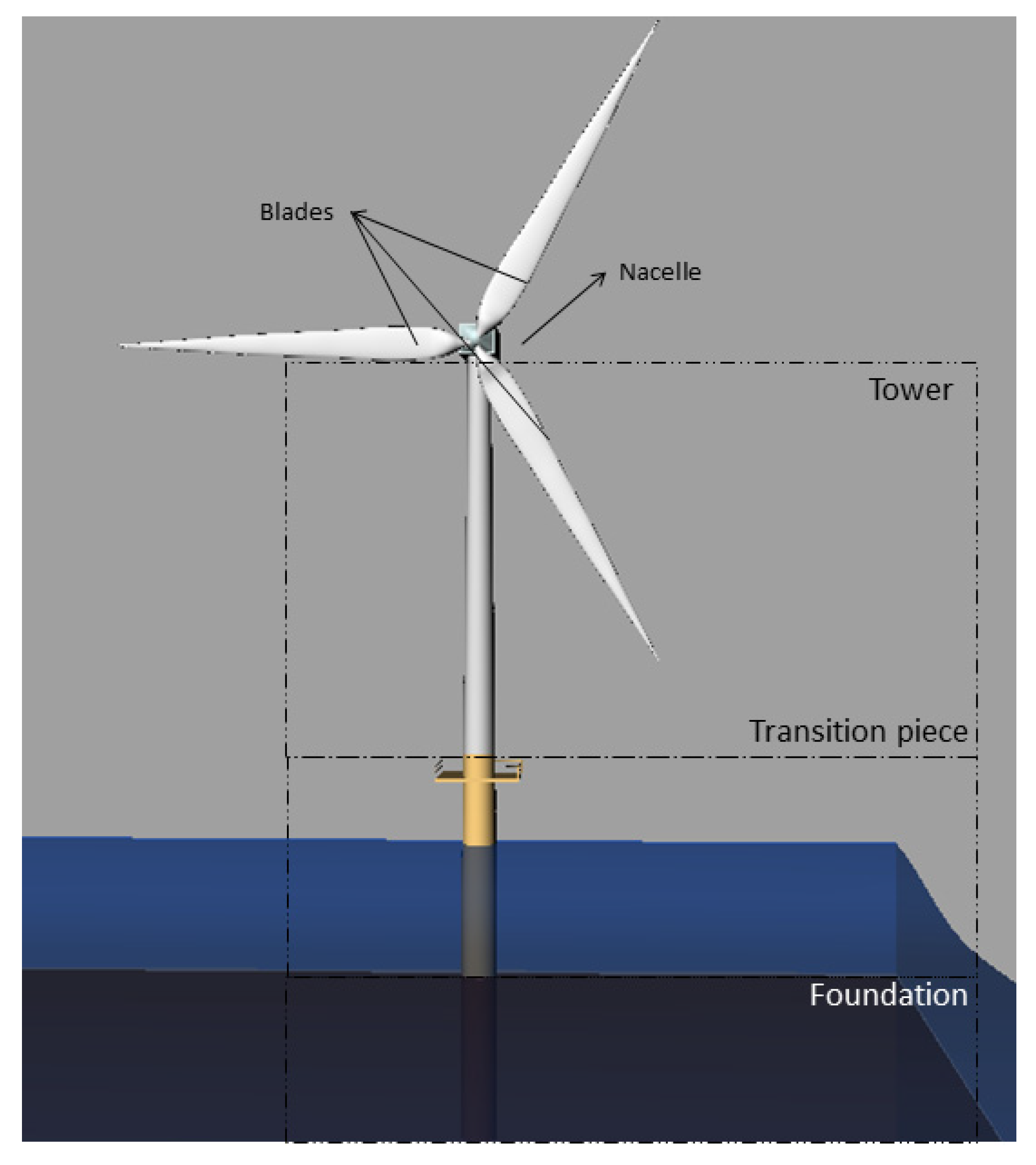
The monopile offshore wind turbines with a 5 MW power capacity are considered a reference ageing offshore wind structure because the monopile support structures are the most commonly used support structure type. A typical monopile OWT is illustrated in Figure 2, and Table 1 shows the characteristics of the monopile OWT.
The techno-economic life extension assessment for offshore wind assets calculates the mean return based on the assumption that the offshore wind asset is appreciated based on the return on asset obtained annually. Because it is assumed that the offshore wind asset does not require any debt to fund its investment, it is reasonable to take that the risk premium is directly proportional to the variance from the mean value of returns, which can be derived by reversing the capital asset pricing formula to estimate the standard beta and, in turn, the standard deviation.
The future earnings/cash flow of an offshore wind asset requires revenue and operational cost estimation. The revenue can be calculated by multiplying expected energy production by the feed-in tariff. The operating cost can be estimated using empirical formulae based on the operational intensity and wind turbine capacity. It is worth mentioning that the estimates made for future earnings rely heavily on the assumption and the success of empirical models used in the present study.
The present study considers the variables affecting the free cash flow within the scope of a semi-quantitative risk-based analysis based on the likelihood of failing to obtain the predicted future earnings.
These premiums are calibrated depending on the characteristics of the life extension project and the economic environment under which the project is consented. The spread/corporate premium consists of equally-weighted premium components covering possible risks concerning obtaining expected free cash flow such as life extension project, project owner, microeconomics, macroeconomics, energy sector and financial market.
In the present study, the risk-free rate is assumed to be 1.5%, the market return is 8.7%, and the volatility measure is 1.12. The variables considered in the free cash flow analysis and the extent to which these variables affect the interest rate are given in Table 2. The details of the techno-economic life extension assessment can be found in [30].
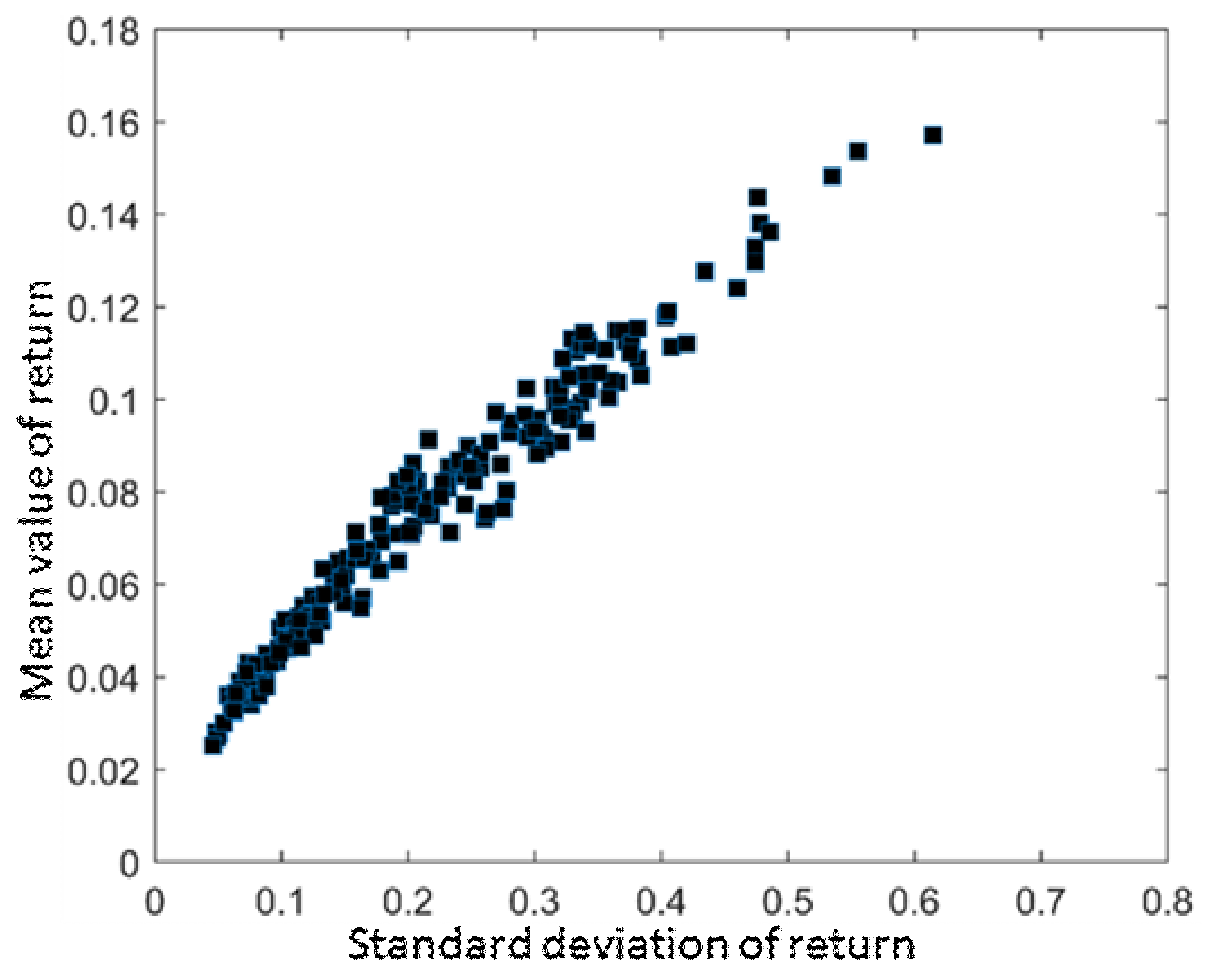
Figure 3 presents the results of the techno-economic analysis for different life extension projects over a risk (standard deviation of return on equity)—return (mean value of return on equity) diagram. The analysis is conducted for 200 life extension projects uniquely characterised based on the variables given in Table 2. The results show a pattern that complies with the expected high-risk high-return model to a certain point, and beyond that point, a higher risk cannot produce a higher return. This phenomenon is explained in economics as “the law of diminishing marginal returns”, which implies that after some certain level of capacity is reached, having an additional risk factor will indeed yield a minor change in return. On the other hand, being too risk-averse could cause the project to not produce any viable return. An efficient frontier is established for the life extension project to guide life extension management in light of these considerations.
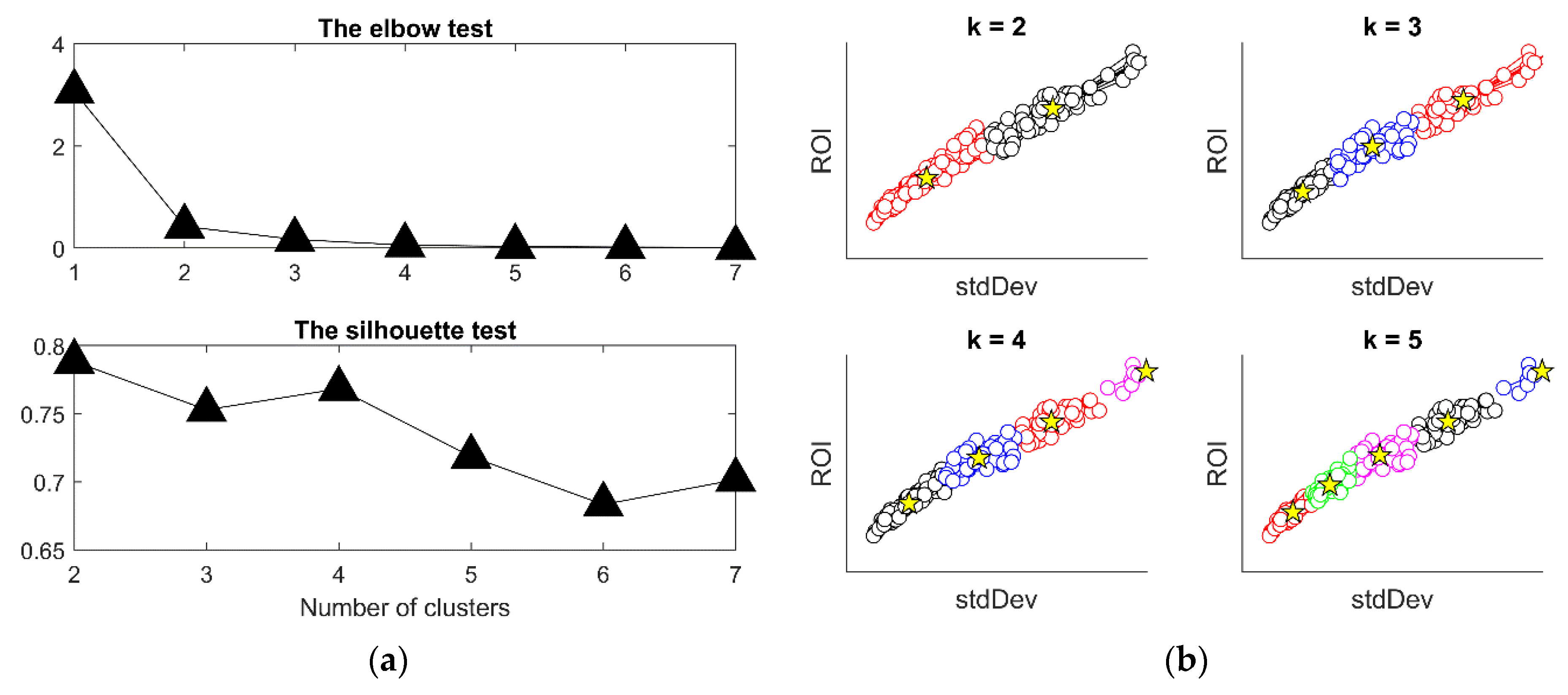
The results of the techno-economic analysis are used to classify the offshore wind turbine. To this end, the k-means unsupervised machine learning (ML) algorithm is employed. Unlike supervised machine learning, the success rate of the k-means algorithm cannot be evaluated by training and testing errors. Instead, the k-means ML algorithm employs quantitative and qualitative metrics to measure the performance of the ML algorithm. In this regard, the elbow test, silhouette test and visual inspection are used to measure the success of the classification concerning the number of clusters.
Figure 4a shows quantitative test results in which the minimum elbow test score and the maximum silhouette score are targeted. At times when the quantitative tests result in multiple candidates, a visual test might be helpful. It can be argued that k = 2 or k = 4 are a reasonable choice for the number of clusters; however, the visual test indicates a classification with four groups would make a better choice (see Figure 4b).
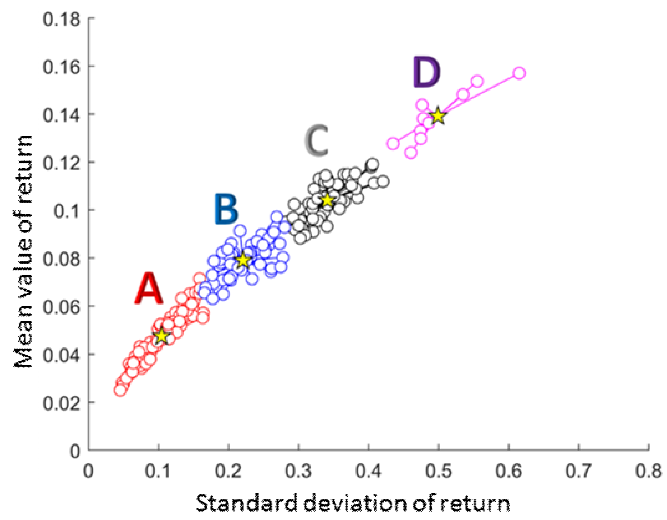
Figure 5 demonstrates the classified offshore wind assets on a risk−return diagram, where the mean value of return denotes return on investment, and the standard deviation indicates the risk. Four groups are identified as Group A, B, C and D. Asset class D is associated with the highest expected return and the highest risk. In contrast, asset class A is associated with the lowest risk and lowest expected return.
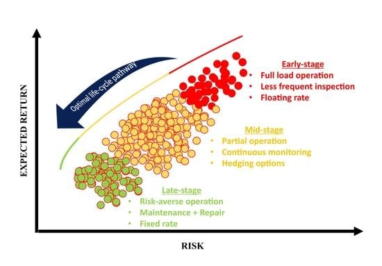
A reasonable scenario would be starting in the region of high risk and high return as Group D. Risk mitigation strategies can be applied to make the overall offshore wind farm less risky asset group zones towards the end of the life extension.
4. Case Studies and Discussion
As a result of the techno-economic analysis followed by the k-means unsupervised ML algorithm, the classified offshore wind assets on a risk−return diagram are obtained. The present section uses the provided data to conduct the mean-variance optimisation for offshore wind assets of different classes (classification). The modern portfolio theory requires the covariance matrix between the offshore wind assets besides the mean value and standard deviation. To this end, a time series of the mean value of returns is generated based on the monthly expected return and standard deviation of each offshore wind asset using sampling as white Gaussian noise. The generated time series are used to estimate the covariance and correlation matrix.
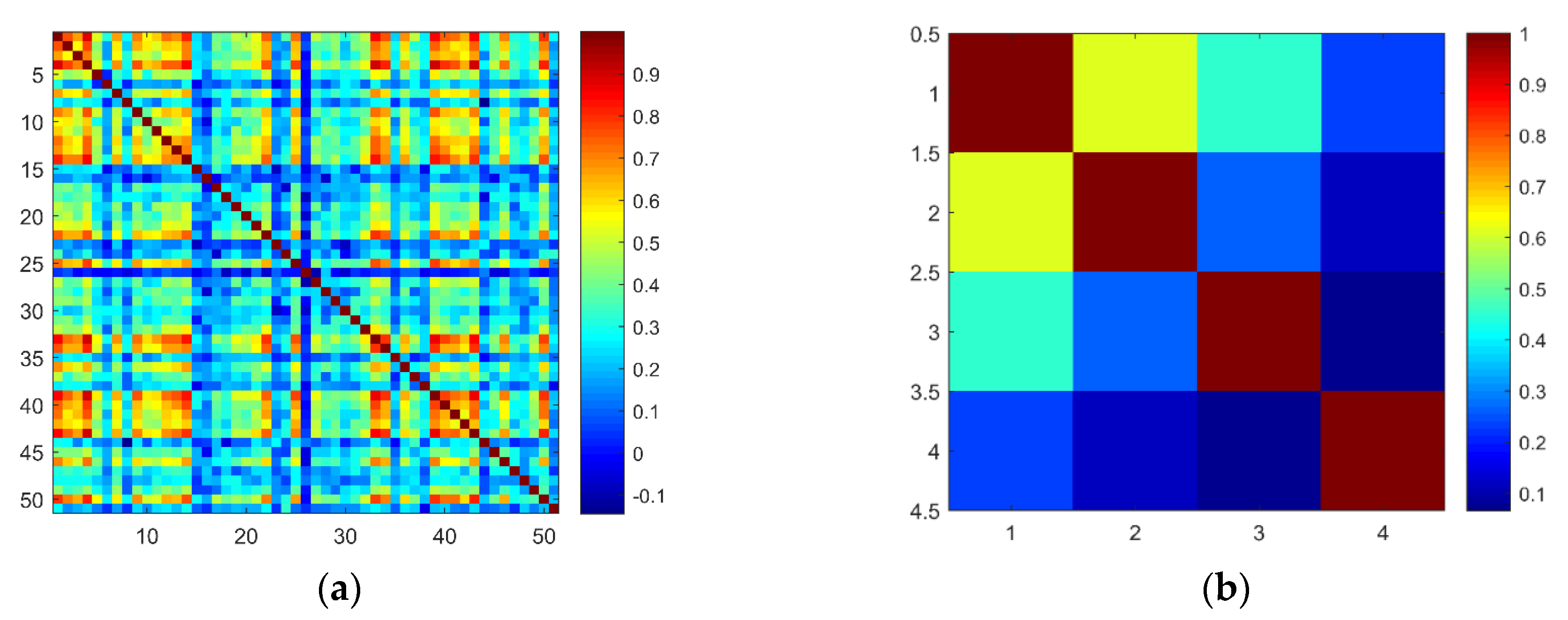
Although the techno-economic analysis resulted in 200 data points, the correlation matrix of 50 offshore wind assets is shown in Figure 6a for better visibility. Figure 6b demonstrates the correlation matrix of four offshore wind turbines deemed representative of four asset groups (A, B, C and D), as identified in the previous section. The correlation value of +1 refers to fully correlated offshore wind assets, and the correlation value of −1 refers to negatively correlated offshore wind assets.
In the choice of the representative offshore wind turbines, it is aimed to have assets with different correlations, assuming that the offshore wind turbines might differ considerably from the wind turbine efficiency and structural condition standpoint after 25 years of service life.
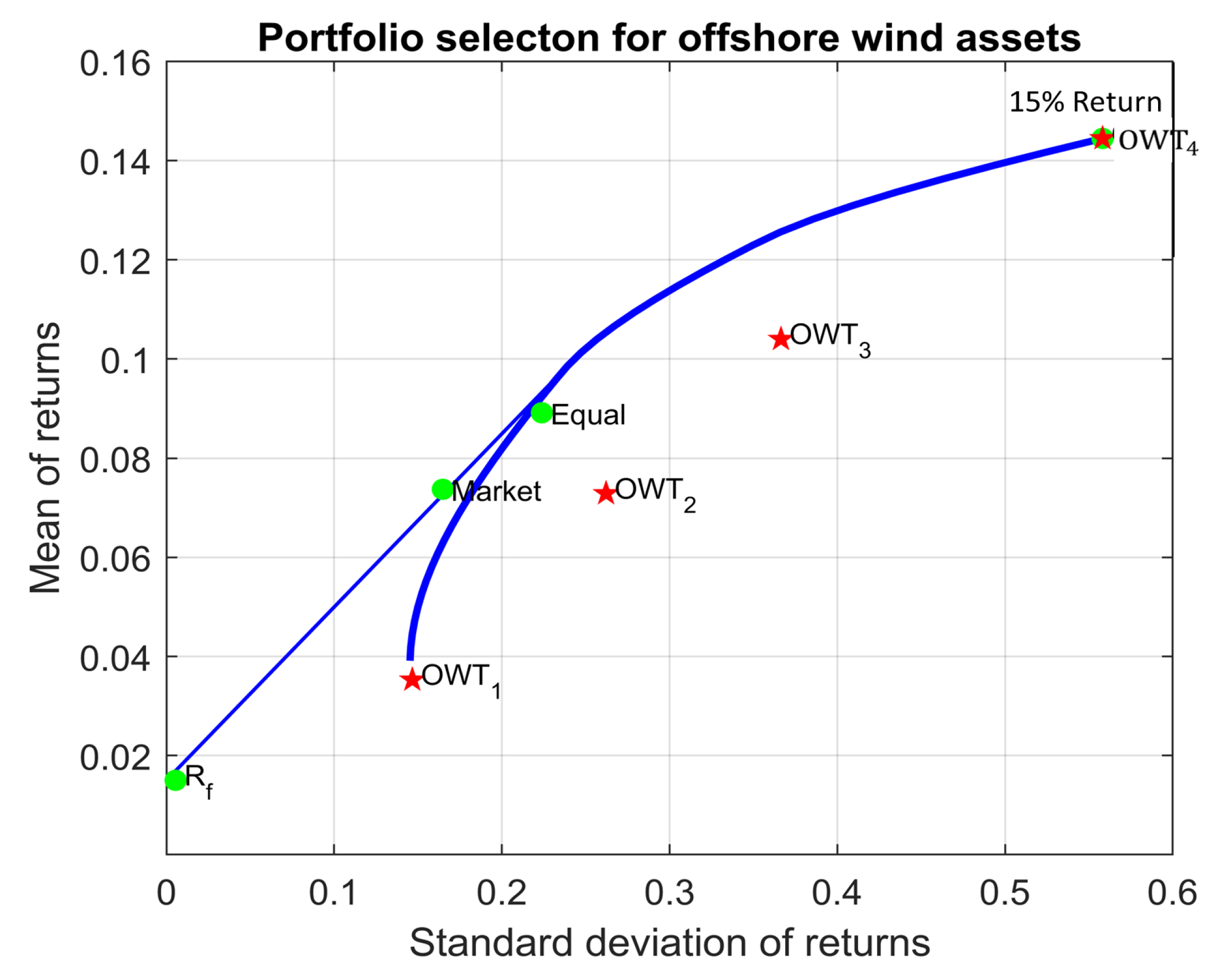
As far as the case studies are concerned, the life extension is considered to have three phases. The first phase is the beginning of the life extension, where the investor can be more risk-tolerant and prefer the portfolio that would bring higher returns.
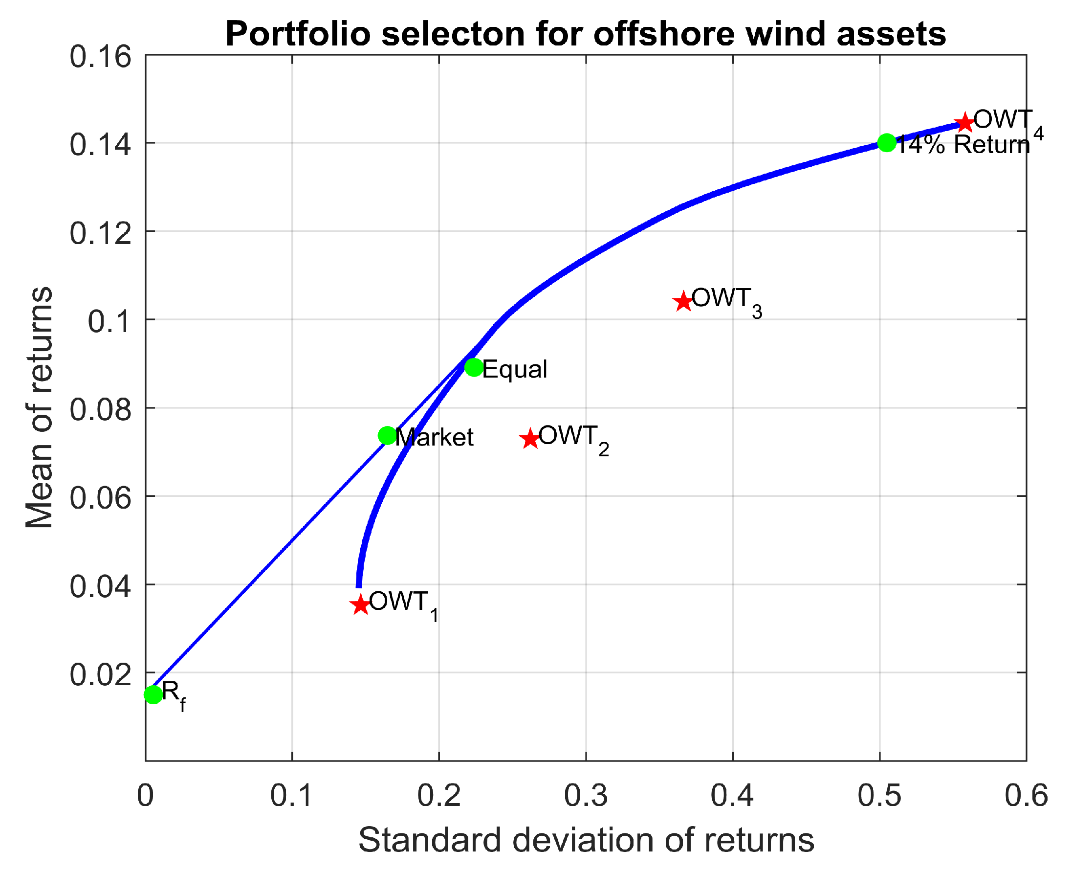
This phase can be investigated in two expected rates of return as 15% and 14%, as in Figure 7 and Figure 8, respectively. The resulting portfolios must be along the efficient frontier. The results indicate that the offshore wind farms must have a significant portion of their offshore wind turbines operating conditions at asset class D (OWT4) to achieve such expected returns.
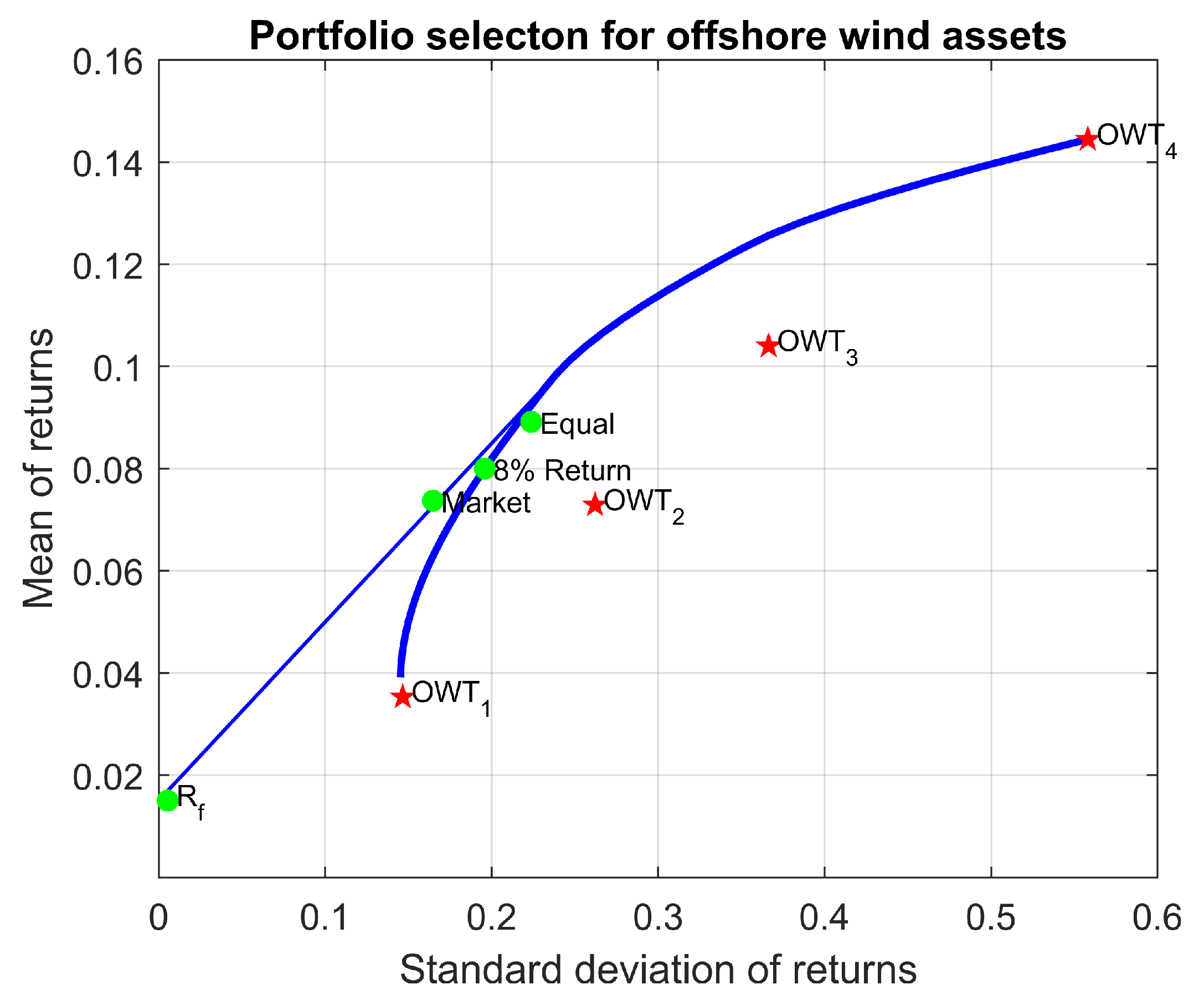
For the second phase, the offshore wind farm is considered to be halfway through the complete life extension. It is reasonable to argue that investors would prefer a less risky operation of the offshore wind farm as the structural conditions are worsening and the capacity factor of the offshore wind farm are decreased. The optimal portfolios on the efficient frontier are demonstrated for 12% and 10% mean value of the return on investment (ROI) in Figure 9 and Figure 10, respectively.
The results show that if the offshore wind turbines of different asset groups were equally weighted, the expected return would be lower than the mean-variance optimisation suggested. For this phase, asset classes B and C outweigh the other asset groups. Nevertheless, it is beneficial to have other asset groups with smaller portions to take advantage of the diversification effect on risk mitigation. It should also be expected that as the correlation between the asset groups increases, the efficient portfolio curve gets closer to the assets, meaning that the overall portfolio risk becomes higher than the portfolio with less correlated asset groups.
The investors’ expectations would be different towards the end of the life extension. As a result of an intensive operation, the offshore wind assets should expect to have more structural integrity issues that need to be attended to by maintenance or even repair. A proactive management approach would be reducing the targeted rate of return, thus the risk.
Figure 11 shows the portfolio on the efficient frontier, which happens to be somewhere between an equally weighted portfolio and the market return in terms of return. Figure 12 shows the portfolio selection that minimises the risk for the available asset groups. Although the low-risk asset class has the largest position in the optimal portfolio, the total risk of the offshore wind farm is less than the asset class A (OWT1), which demonstrates the power of diversification on the offshore wind farm consisting of multiple offshore wind turbines with varying features.
In addition to the portfolios optimised for the different phases of the life extension, decision-makers responsible for the life extension operational management might be interested in acquiring a portfolio of offshore wind assets that will maximise how much excess return is gained for having a risky asset, in other words, risk-adjusted return. The modern portfolio theory introduces this concept through the Sharpe [4] ratio.
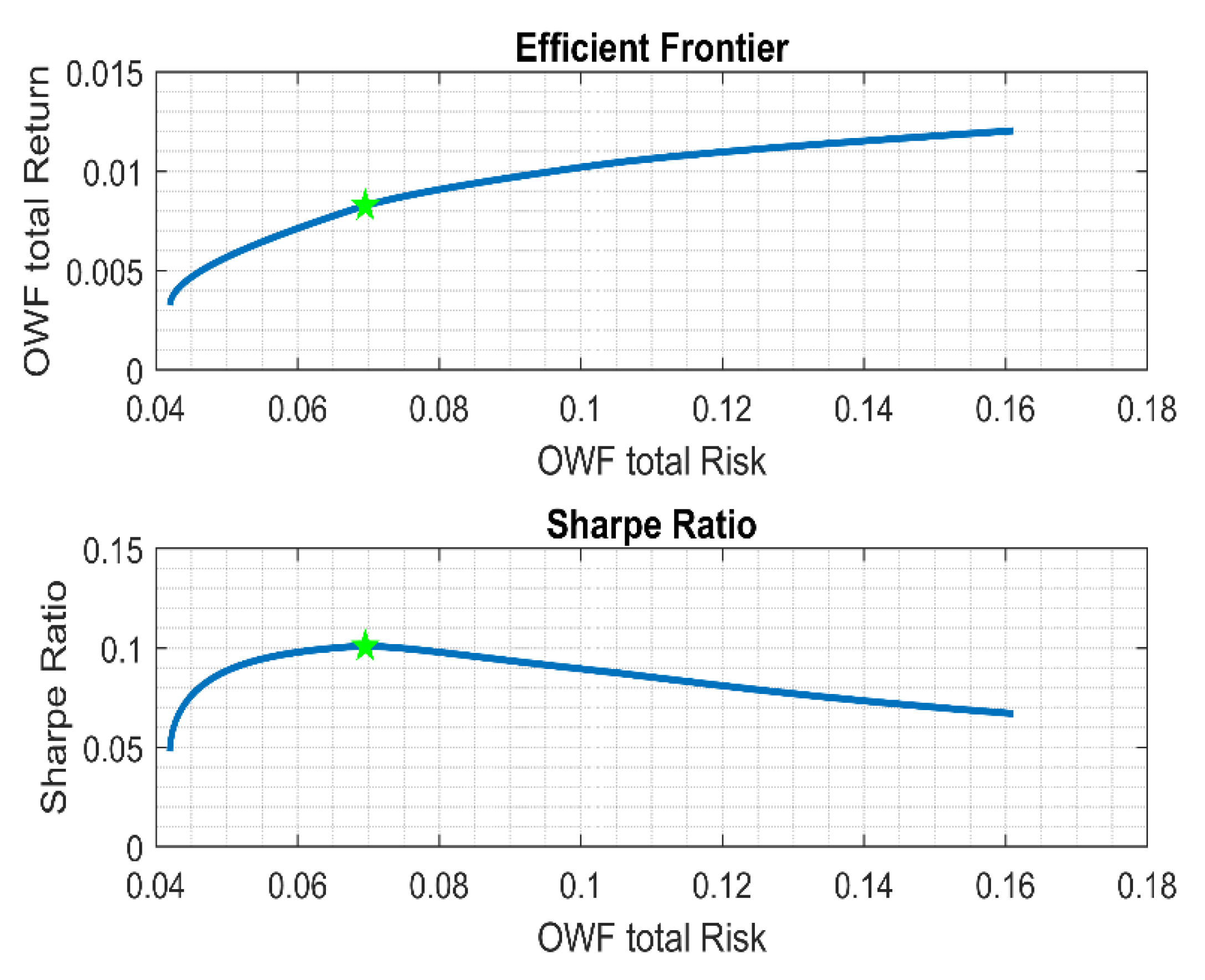
Figure 13 shows the portfolio that maximises the Sharpe ratio and the portfolios generated for the portfolio at the market risk, the equally weighted portfolio and the portfolio targeting 12% return. The Sharpe ratio on the efficient frontier is also the point that intersects with a tangential line connecting to the risk-free asset type. This line is called the capital allocation line for investors who allocate the capital between the Sharpe ratio and risk-free assets in finance, which does not have any place in the present study.
The Sharpe ratio is calculated based on the residual return (mean value of the rate of return—risk-free rate) divided by the standard deviation of the selected portfolio. This calculation is done for every portfolio on the efficient frontier and the portfolio that maximises the Sharpe ratio, therefore the most risk-adjusted return. The result of the optimisation that maximises the Sharpe ratio is presented in Figure 14. The Sharp ratio decreases as the standard deviation of the return or the mean value of return increases because of the marginal diminishing return concept. The marginal diminishing return concept suggests that an investor needs to take higher risks to obtain excess return after the Sharpe ratio.
From the corporate finance point of view, the project’s profitability measures such as the return on an asset, return on equity, return on investment (capital) and return on sales needs to be such a rate that compensates for the appropriate hurdle rate. The hurdle rate reflects the price for taking the risk to earn a given expected return. The generic investment concept is valid for financial, non-financial, corporate funding or project funding. The undeniable principle is to assess the added value (future earnings) brought to the investment (capital), accounting for the opportunity cost (weighted average cost of capital). Depending on the financial activities decided for the project, the performance measure can differ. However, ultimately the decision-makers seek projects/investments that will bring higher returns on the capital than the corresponding cost of capital.
Within the scope of the present work, the analysis is conducted based on the assumptions that the offshore wind farms analysed for the life extension have neither debt nor retained cash from the previous operating period. Based upon this assumption, the cost of capital associated with the offshore wind life extension is defined by the equity risk premium. The performance measure is considered a return on equity, even though equity, total asset, and initial capital would mean the same.
The equity risk premium is the price seen fit for taking the risk. The decision-makers’ view on the macroeconomics, microeconomics, long and short-term corporate strategy, energy market, and competitors inside and outside of the sector would determine the willingness to take the risk. The present study guides the decision-makers regarding the life extension of offshore wind farms. The asset type categorised as “high-risk high-return” is recommended for the beginning of the life extension; however, the decision-makers are urged to minimise the risk towards the end of the life extension to preserve its asset and avoid downside risk.
The present study analysed the riskiness of a life extension of an offshore wind farm via the perspective of two schools of thought. The first school of thought takes the risk as the variance of return around an expected return, which is caused by the variability of the factors affecting the operating income of the offshore wind farm. The latter denotes the risk as any action taken other than having the well-diversified portfolio that maximises the Sharpe ratio. The second definition of risk assumes that the operators would minimise the risk of return by being well-diversified between the offshore wind assets; the well-diversified portfolio of offshore wind turbines eliminates all the idiosyncratic risk associated with the individual asset and the systematic risk associated with the overall offshore wind farm and site remains. This means that for any chosen portfolio other than the well-diversified portfolio, there must be compensation.
The scope of the present study can be extended in the future by incorporating the capital asset pricing model, CAPM, within the modern portfolio theory to provide a relative measure of the risk premium for a different combination of asset groups accounting for macroeconomics, microeconomics, energy sector strength, and political and environmental sentiment. Such studies would allow for a more comprehensive look at the life-extension decisions related to operating, investing and financing and help to have better judgements on the appropriate equity premium, the weighted average cost of capital and the hurdle (discount) rate, which has utmost importance for project finance.
5. Conclusions
The present study developed a risk-based approach to finding optimal life extension management strategies for offshore wind farms based on Markowitz’s modern portfolio theory. The techno-economic life extension assessment was conducted considering the offshore wind turbines as cash-producing tangible assets; consequently, the mean value of return on investment and the deviation from the mean value were obtained to construct the risk−return diagram. The K-means unsupervised machine learning algorithm classified four different asset groups for which the mean-variance optimisation was conducted. Finally, the case studies were generated considering different stages of the extended service life and the investors’/decision-makers’ expectation.
The results of the mean-variance analysis indicated that a portfolio consisting of OWTs of different asset classes provides lower risk-taking for a required rate of return than an equally-weighted portfolio. This conclusion is valid for all the case studies except for the required return of 15% and above and supports the argument that the diversification between different offshore wind asset classes almost always helps with the risk mitigation during the life extension. However, the contribution of each asset group to the overall portfolio changes with the required return, which varies depending on the life extension phase of the offshore wind farm.
In addition to case studies created for different phases of life extension, the present study optimised a portfolio that maximises the ratio between the excess return gained for taking risk (Sharpe ratio). The portfolio with the maximum Sharpe ratio was estimated to be a 10% mean value of return on investment with a 24% standard deviation of return on investment. The decision-makers/investors must consider the portfolio return and risk and compare this with the defined hurdle rate before accepting the terms of the life extension project.
Furthermore, the outcome of this study enables the creation of a roadmap for sustainable and efficient life-cycle and extension management decisions by tuning the control parameters such as the operational intensity, the number of active offshore wind assets, risk hedging options, repowering or decommissioning.
Author Contributions
Conceptualisation, B.Y. and Y.G.; methodology, B.Y. and Y.G.; coding, B.Y.; validation, B.Y. and Y.G.; formal analysis, B.Y.; investigation, B.Y. and Y.G.; resources, B.Y.; data curation, B.Y.; writing—original draft preparation, B.Y. and Y.G.; writing—review and editing, Y.G.; visualisation, B.Y.; supervision, Y.G. All authors have read and agreed to the published version of the manuscript.
Funding
This research received no external funding.
Data Availability Statement
The data presented in this study are available within the article.
Acknowledgments
This work was performed within the Strategic Research Plan of the Centre for Marine Technology and Ocean Engineering (CENTEC), which is financed by the Portuguese Foundation for Science and Technology (Fundação para a Ciência e Tecnologia-FCT) under contract UIDB-UIDP/00134/2020.
Conflicts of Interest
The authors declare no conflict of interest.
References
- Markowitz, H.M. Portfolio selection. J. Financ. 1952, 7, 77–91. [Google Scholar]
- Markowitz, H.M. Markowitz revisited. Financ. Anal. J. 1976, 32, 47–52. [Google Scholar] [CrossRef]
- Tobin, J. Liquidity preference as behavior towards risk. Rev. Econ. Stud. 1958, 25, 65–86. [Google Scholar] [CrossRef]
- Sharpe, W.F. Mutual fund performance. J. Bus. 1966, 39, 119–138. [Google Scholar] [CrossRef]
- Treynor, J. The investment value of brand franchise. Financ. Anal. J. 1999, 55, 27–34. [Google Scholar] [CrossRef]
- Treynor, J. Zero-sum. Financ. Anal. J. 1999, 55, 8–12. [Google Scholar] [CrossRef]
- Maier-Paape, S.; Zhu, Q.J. A general framework for portfolio theory—Part II: Drawdown risk measures. Risks 2018, 6, 76. [Google Scholar] [CrossRef] [Green Version]
- Maier-Paape, S.; Zhu, Q.J. A general framework for portfolio theory—Part I: Theory and various models. Risks 2018, 6, 53. [Google Scholar] [CrossRef] [Green Version]
- Green, R.; Vasilakos, N. The economics of offshore wind. Energy Policy 2011, 39, 496–502. [Google Scholar] [CrossRef]
- Levitt, A.C.; Kempton, W.; Smith, A.P.; Musial, W.; Firestone, J. Pricing offshore wind power. Energy Policy 2011, 39, 6408–6421. [Google Scholar] [CrossRef]
- Blanco, M.I. The economics of wind energy. Renew. Sustain. Energy Rev. 2009, 13, 1372–1382. [Google Scholar] [CrossRef]
- Chaves-Schwinteck, P. The Modern Portfolio Theory Applied to Wind Farm Investments. Ph.D. Thesis, Universität Oldenburg, Oldenburg, Germany, 2013. [Google Scholar]
- Dunlop, J. Modern portfolio theory meets wind farms. J. Priv. Equity 2004, 7, 83–95. [Google Scholar] [CrossRef]
- Drake, B.; Hubacek, K. What to expect from a greater geographic dispersion of wind farms?—A risk portfolio approach. Energy Policy 2007, 35, 3999–4008. [Google Scholar] [CrossRef] [Green Version]
- Roques, F.; Hiroux, C.; Saguan, M. Optimal wind power deployment in Europe—A portfolio approach. Energy policy 2010, 38, 3245–3256. [Google Scholar] [CrossRef] [Green Version]
- Rombauts, Y.; Delarue, E.; D’haeseleer, W. Optimal portfolio-theory-based allocation of wind power: Taking into account cross-border transmission-capacity constraints. Renew. Energy 2011, 36, 2374–2387. [Google Scholar] [CrossRef]
- Chupp, B.A.; Hickey, E.; Loomis, D.G. Optimal wind portfolios in Illinois. Electr. J. 2012, 25, 46–56. [Google Scholar] [CrossRef]
- Costa-Silva, L.V.L.; Almeida, V.S.; Pimenta, F.M.; Segantini, G.T. Time span does matter for offshore wind plant allocation with modern portfolio theory. Int. J. Energy Econ. Policy 2017, 7, 188–193. [Google Scholar]
- Hu, J.; Harmsen, R.; Crijns-Graus, W.; Worrell, E. Geographical optimisation of variable renewable energy capacity in China using modern portfolio theory. Appl. Energy 2019, 253, 113614. [Google Scholar] [CrossRef]
- Marrero, G.A.; Puch, L.A.; Ramos-Real, F.J. Mean-variance portfolio methods for energy policy risk management. Int. Rev. Econ. Financ. 2015, 40, 246–264. [Google Scholar] [CrossRef]
- Arnesano, M.; Carlucci, A.P.; Laforgia, D. Extension of portfolio theory application to energy planning problem—The Italian case. Energy 2012, 39, 112–124. [Google Scholar] [CrossRef]
- Cunha, J.; Ferreira, P.V. Designing electricity generation portfolios using the mean-variance approach. Int. J. Sustain. Energy Plan. Manag. 2014, 4, 17–30. [Google Scholar]
- Thomaidis, N.S.; Santos-Alamillos, F.J.; Pozo-Vázquez, D.; Usaola-García, J. Optimal management of wind and solar energy resources. Comput. Oper. Res. 2016, 66, 284–291. [Google Scholar] [CrossRef] [Green Version]
- Schmidt, J.; Lehecka, G.; Gass, V.; Schmid, E. Where the wind blows: Assessing the effect of fixed and premium based feed-in tariffs on the spatial diversification of wind turbines. Energy Econ. 2013, 40, 269–276. [Google Scholar] [CrossRef]
- Delarue, E.; De Jonghe, C.; Bellman’s, R.; D’haeseleer, W. Applying portfolio theory to the electricity sector: Energy versus power. Energy Econ. 2011, 33, 2–23. [Google Scholar] [CrossRef]
- deLlano-Paz, F.; Calvo-Silvosa, A.; Antelo, S.I.; Soares, I. Energy planning and modern portfolio theory: A review. Renew. Sustain. Energy Rev. 2017, 77, 636–651. [Google Scholar] [CrossRef]
- Yeter, B.; Garbatov, Y.; Soares, C.G. Risk-based multi-objective optimisation of a monopile offshore wind turbine support structure, OMAE2017-61756. In Proceedings of the 36th International Conference on Ocean, Offshore and Arctic Engineering, OMAE17, Trondheim, Norway, 25–30 June 2017. [Google Scholar]
- Yeter, B.; Garbatov, Y.; Soares, C.G. Risk-based life-cycle assessment of offshore wind turbine support structures accounting for economic constraints. Struct. Saf. 2019, 81, 101867. [Google Scholar] [CrossRef]
- Yeter, B.; Garbatov, Y.; Soares, C.G. Risk-based maintenance planning of offshore wind farms. Reliab. Eng. Syst. Saf. 2020, 202, 107062. [Google Scholar] [CrossRef]
- Yeter, B.; Garbatov, Y.; Soares, C.G. Techno-economic analysis for life extension certification of offshore wind assets using unsupervised machine learning. 2021. submitted. [Google Scholar]
Figure 1.
Flow chart for the development of life extension classification.

Figure 2.
Typical monopile OWT structure.

Figure 3.
Risk−return diagram.

Figure 4.
Quantitative (a) and qualitative test (b) for the k-means clustering.

Figure 5.
Classification of life extension projects in four groups (A–D) with the centroids of the classified groups (Yellow star).
Figure 5.
Classification of life extension projects in four groups (A–D) with the centroids of the classified groups (Yellow star).

Figure 6.
Correlation matrix for 50 simulated offshore wind assets (a) and four representative assets (b).
Figure 6.
Correlation matrix for 50 simulated offshore wind assets (a) and four representative assets (b).

Figure 7.
Mean value of returns as a function of standard deviation, 15% return and equal weights.

Figure 8.
Mean value of returns as a function of standard deviation, 14% return and equal weights.

Figure 9.
Mean value of ROI as a function of standard deviation, 12% return and equal weights.

Figure 10.
Mean value of ROI as a function of standard deviation, 10% return and equal weights.

Figure 11.
Mean value of ROI as a function of standard deviation, 8% return and equal weights.

Figure 12.
Mean value of ROI as a function of standard deviation, minimum risk (14.55%).

Figure 13.
Optimal portfolio at the maximum Sharpe ratio.

Figure 14.
Sharpe ratio over different portfolios on efficient frontier.


| Wind turbine | 5 MW NREL |
| Rated wind speed | 11.8 m/s |
| The expected value of wind speed | 9 m/s |
| Hub height (from the MSL) | 86 m |
| Water depth (from the MSL) | 40 m |
| Turbulence intensity | 0.12 |
| Integral length scale | 340 m |
| Thrust coefficient (N/(m/s)) | 0.73 |
| Structural and aerodynamic damping | 4% and 1% |
| Natural frequency | 0.281 Hz |
| Diameter of support structure | 6 m |
| Thickness of support structure | 50 mm |
| Material constant | 5.21 × 10⁻¹³ |
| Material exponent | 3 |
| Threshold stress intensity factor | 2 MPa·ml/2 |
| Critical stress intensity factor | 69 MPa·ml/2 |
| Yield stress | 355 MPa |
| Plate breadth | 0.1 m |
| Sigmoid slope | 0.2 |
| Shift parameter | 0.01 |
Table 2.
Characteristic of variables involved in the intrinsic value analysis.
| Variables | E [] | COV (%) | Distribution |
| Expected wind speed (m/s) | 10 | 10 | Weibull |
| Operation intensity | 0.75 | 10 | Normal |
| Wind farm size (unit) | 30 | 20 | Uniform |
| Life extension (year) | 20 | 40 | Uniform |
| Management efficiency | 0.85 | 10 | Normal |
| Availability and capacity factor | 0.95 and 0.44 | 10 | Normal |
| Measured crack size (m) | 0.010 | 20 | Lognormal |
| Feed-in tariff (€/MWh) | 120 | 20 | Normal |
| Safety class | 5 | 50 | Uniform |
Publisher’s Note: MDPI stays neutral with regard to jurisdictional claims in published maps and institutional affiliations. |
© 2021 by the authors. Licensee MDPI, Basel, Switzerland. This article is an open access article distributed under the terms and conditions of the Creative Commons Attribution (CC BY) license (https://creativecommons.org/licenses/by/4.0/).
Share and Cite
MDPI and ACS Style
Yeter, B.; Garbatov, Y. Optimal Life Extension Management of Offshore Wind Farms Based on the Modern Portfolio Theory. Oceans 2021, 2, 566-582. https://0-doi-org.brum.beds.ac.uk/10.3390/oceans2030032
AMA Style
Yeter B, Garbatov Y. Optimal Life Extension Management of Offshore Wind Farms Based on the Modern Portfolio Theory. Oceans. 2021; 2(3):566-582. https://0-doi-org.brum.beds.ac.uk/10.3390/oceans2030032
Chicago/Turabian StyleYeter, Baran, and Yordan Garbatov. 2021. "Optimal Life Extension Management of Offshore Wind Farms Based on the Modern Portfolio Theory" Oceans 2, no. 3: 566-582. https://0-doi-org.brum.beds.ac.uk/10.3390/oceans2030032