Article

Cold-Water Coral Reefs in the Langenuen Fjord, Southwestern Norway—A Window into Future Environmental Change

1
GEOMAR Helmholtz Centre for Ocean Research Kiel, Wischhofstraße 1-3, 24148 Kiel, Germany
2
Institute of Marine Research in Norway (IMR), Nordnesgaten 50, 5005 Bergen, Norway
3
Institute of Marine Research in Norway, Fram Centre, 9007 Tromsø, Norway
*
Author to whom correspondence should be addressed.
Submission received: 30 October 2020 / Revised: 14 May 2021 / Accepted: 10 August 2021 / Published: 25 August 2021

Abstract

:
Ocean warming and acidification pose serious threats to cold-water corals (CWCs) and the surrounding habitat. Yet, little is known about the role of natural short-term and seasonal environmental variability, which could be pivotal to determine the resilience of CWCs in a changing environment. Here, we provide continuous observational data of the hydrodynamic regime (recorded using two benthic landers) and point measurements of the carbonate and nutrient systems from five Lophelia pertusa reefs in the Langenuen Fjord, southwestern Norway, from 2016 to 2017. In this fjord setting, we found that over a tidal (<24 h) cycle during winter storms, the variability of measured parameters at CWC depths was comparable to the intra-annual variability, demonstrating that single point measurements are not sufficient for documenting (and monitoring) the biogeochemical conditions at CWC sites. Due to seasonal and diurnal forcing, parts of the reefs experienced temperatures up to 4 °C warmer (i.e., >12 °C) than the mean conditions and high CT concentrations of 20 µmol kg−1 over the suggested threshold for healthy CWC reefs (i.e., >2170 µmol kg−1). Combined with hindcast measurements, our findings indicate that these shallow fjord reefs may act as an early hotspot for ocean warming and acidification. We predict that corals in Langenuen will face seasonally high temperatures (>18 °C) and hypoxic and corrosive conditions within this century. Therefore, these fjord coral communities could forewarn us of the coming consequences of climate change on CWC diversity and function.

1. Introduction

Cold-water coral (CWC) reefs form complex habitats in the deep sea, supporting rich associated fauna [1,2,3,4]. They play a major role in the circulation of organic carbon in the deep sea [5,6]. The reefs are recognized as vulnerable marine ecosystems (VMEs) by the United Nations [7] and as threatened and declining habitats by the OSPAR commission [8]. Warming and acidifying waters (i.e., decreasing pH and aragonite saturation state, ΩAr) are predicted to pose imminent and serious threats to CWC reefs within the next decades [9,10]. Hence, there has been an intensified focus to assess the range of biogeochemical and physical conditions tolerated by CWCs in situ [11,12,13,14,15,16] and in laboratory conditions [17,18,19,20,21]. Finally, a focus is on determining the baseline for optimal conditions for coral growth and reef development [22]. However, there is very little data on the small-scale temporal and spatial variability of biogeochemical and physical conditions in CWC settings, which could be pivotal in understanding their resilience to climate change, as observed for tropical coral reefs [23].
In the North Atlantic, CWC reefs are most commonly build by Lophelia pertusa (syn. Desmophyllum pertusum [24]), with around a third of all known L. pertusa occurrences being from Norwegian waters [25]. L. pertusa reefs are generally found on and around elevated bathymetric structures such as mounds, offshore banks, seamounts, and sills [26,27,28,29,30], where relatively strong bottom flow associated with those structures enhances the flux of food particles [22,31,32,33] and facilitates sediment removal from CWCs or the seafloor to provide suitable settlement substrates for coral larvae [25,34]. While local hydrodynamics are important in regulating the distribution of CWCs, water column characteristics such as temperature, nutrient availability, carbonate chemistry (mainly aragonite saturation, ΩAr), and oxygen levels [2,12,15,35] act as additional and strong drivers in regulating coral growth. The latter two are vital in maintaining calcification and aerobic metabolism in corals, while low-temperature regimes decelerate food decay (enhancing food availability) and reduce metabolic energy demands [36].
Rising global ocean temperatures have been observed throughout the water column since the 1960s [37]. In coastal Norway, rapid warming of the Norwegian coastal water (NCW) and the North Atlantic water (NAW, SA < 35 g kg−1) in mid-layer waters has been reported since the 1980s [38]. Ocean warming is expected to affect both the fitness and the geographical distribution of many marine species in the coming decades. CWCs are usually found in waters with temperatures <12 °C [13,29,39], but occasionally they thrive in warmer waters of ~15 °C [15,40]. Even though CWCs can tolerate substantial fluctuations in temperature [41,42], a rise of only 2 °C for a few hours will significantly increase its energy demands [36,41], which could deplete energy stores if they are not met by increased food availability and/or uptake rates [35]. Ocean warming can also indirectly affect CWCs by changing primary production patterns [43] and reducing oxygen availability [44]. In southwestern Norway, the reduction in oxygen concentration has been ~0.5 mL L−1 per decade over the past 40 years in the fjord basin waters [45].
Long-term decreasing trends of pH and aragonite saturation have been observed in the open ocean around the globe [46,47] as well as in coastal waters off Norway. Currently, the aragonite saturation horizon (ASH, ΩAr < 1) of the Norwegian Sea is at ~2000 m depth. At these depths, an annual decrease of 0.003 in ΩAr and 0.008 in pH has been observed between 2007 and 2017 [48]. The observed decrease inside the fjords, where ΩAr is currently >1 across the water column, is larger. A two-fold annual decrease of 0.007 in ΩAr and of 0.02 in pH compared to offshore and 2000 m depth has been observed at bottom water depths of ~670 m in Korsfjorden south of Bergen between 2007 and 2017 [48]. Calcifying marine organisms such as CWCs will be directly impacted by the shoaling of the ASH. Below the ASH depth, mineral dissolution occurs, dissolving the exposed dead coral framework that constitutes a major component of the reef, and waters are less favorable for skeletal growth [29,49,50]. The skeleton of L. pertusa is based on aragonite, the most labile form of calcium carbonate. Hence, the reefs are considered particularly susceptible to a decreasing ΩAr. If current trends continue at unchanged rates, the ASH is estimated to reach the surface by the year 2070 ± 10 in southwestern Norwegian fjords [51], while deeper waters (>600 m) off Norway will become corrosive already within the next 20 years [48]. Most of the Norwegian CWCs are observed in between these depths, so they are likely to experience corrosive conditions in the next 20–50 years.
The seasonal changes in carbonate chemistry in high latitude surface waters are driven by temperature, salinity, air-sea CO2 exchange, formation and decay of organic matter, and advection and vertical mixing with deeper, carbon-rich coastal water [51]. In western Norwegian fjords, the spring phytoplankton bloom yields maximum pH and reduced dissolved inorganic carbon (CT) values. Seasonal ΩAr variations align with those of surface temperature, both peaking in late summer. This seasonal forcing also affects the carbonate chemistry at the depths of living CWCs (i.e., 80–250 m). Generally, the CT and carbon dioxide (CO2) concentrations increase with depth. This is caused by enhanced respiration and remineralization of organic matter, which also yield to decreased pH [48,52,53,54,55]. Apart from Findlay et al. (2014) [53], who provided a high-resolution nutrient and carbonate chemistry data over a tidal cycle showing the influence of local upwelling for Scottish and Irish CWC reefs, very little data exist on diurnal variability and not least the seasonal dynamics of carbonate chemistry for deep waters. At present, carbonate chemistry and nutrient data are primarily available from global data sets [56,57]. These are useful for making large-scale habitat predictions [13,58], but they lack the fine-scale spatial and temporal coverage that is required to understand the baseline of physicochemical dynamics around CWC reefs that plays a key role in determining the resilience of CWC reefs to future climate change.
This study investigated the natural variability of biogeochemical and physical conditions at five CWC reefs located within a narrow fjord in western Norway. This was achieved by collating water column measurements of carbonate chemistry and inorganic nutrient parameters for multiple stations and timepoints over 1.5 years and combining those with high temporal resolution data from two benthic observatories deployed at one of the reefs. Comparisons of environmental data from reefs growing on vertical walls with those growing on the fjord floor were used to elucidate the relative importance of topography-flow interaction and biogeochemical conditions for CWC occurrences.

2. Materials and Methods
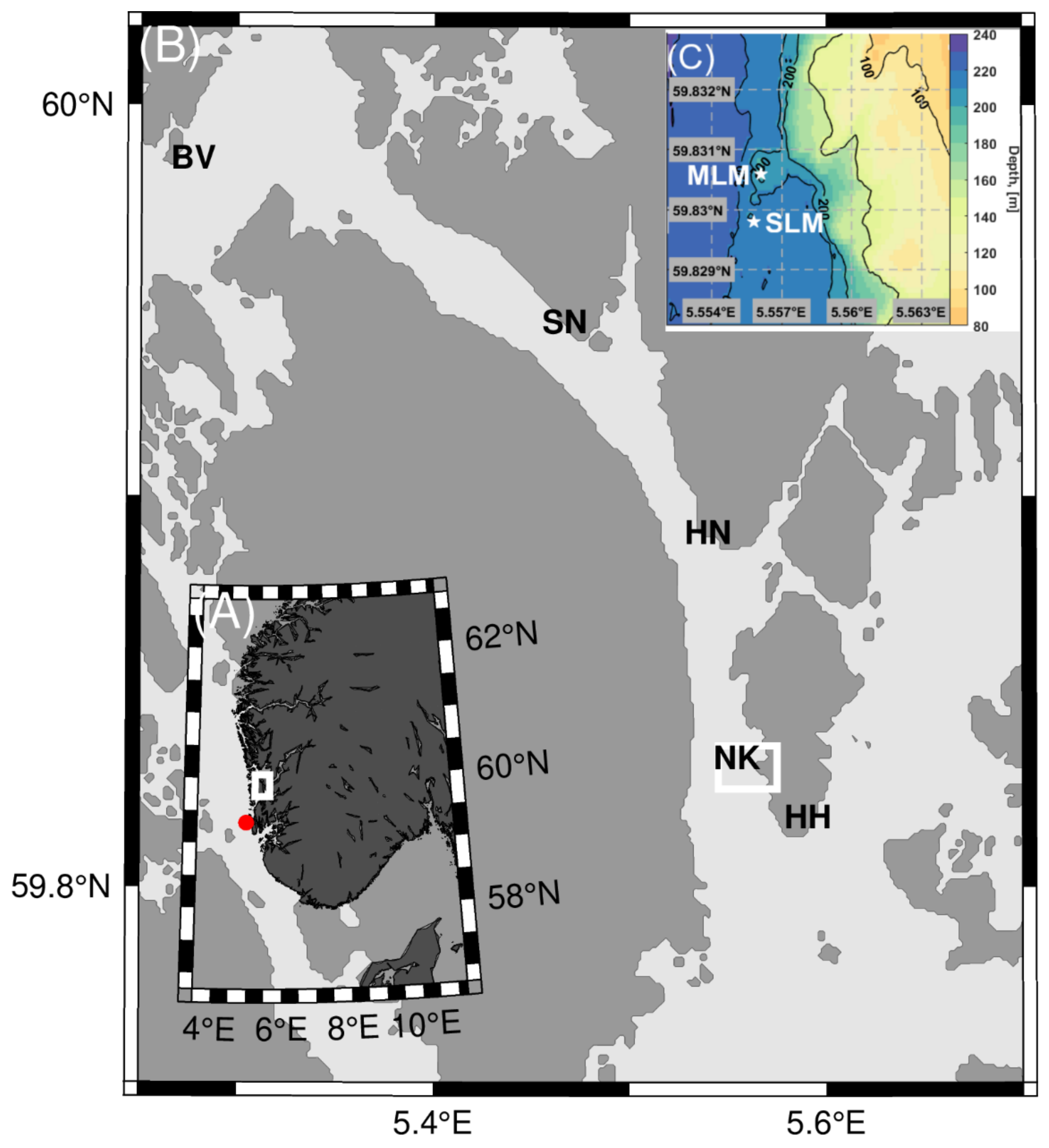
2.1. Study Site

The Langenuen Fjord in southwestern Norway, south of Bergen (Figure 1), is a 35 km long north-south trending water passage connecting the Korsfjorden with the Hardangerfjord. The system opens up to the Atlantic through Korsfjorden at its northern edge, through Selbjørnsfjorden in the central parts, and through Bømlafjorden at its southern end. Langenuen is ~300 m deep. The deepest point measures 568 m and is located in the northern portion between the islands of Huftarøy and Reksteren. The average width of the fjord is 2.9 km in the northern section and 1.7 km in the southern section. The fjord acts as an ocean water inlet to the Hardangerfjord [59]. It hosts several L. pertusa-dominated CWC reefs on the eastern side of the fjord, at depths between 80 and 240 m [60,61]. This study concentrates on five of them in two different settings: corals covering an elevated topographic feature on the fjord bottom here called “bank reef” and corals living on steep walls or cliffs, “wall reefs”. The two bank reefs are Nakken (NK, 59.830° N, 5.550° E) and the northernmost site Bekkjarvik (BV, 59.983° N, 5.276° E). The southernmost site Huglhammaren near the main sill of the Hardangerfjord (HH, 59.815° N, 5.590° E), Straumsneset (SN, 59.941° N, 5.467° E), and Hornaneset (HN, 59.890° N, 5.539° E) are wall reefs on the near-vertical fjord wall. Sites NK and SN are previously described by Fosså et al. (2015) [60].

2.2. Water Column Measurements

Water samples were taken at several depths using a 12-bottle Niskin rosette (Ro) system. For water column hydrography profiling, an instrument measuring in situ conductivity, temperature, and pressure (CTD) attached to the water sampling system was used. A total of 12 CTD and 52 CTD/Ro (CTD/rosette water sampling) casts were carried out across the CWC sites (HH, NK, HN, SN, BK). Measurements were taken during six cruises between February 2016 and August 2017, onboard RV Håkon Mosby, RV Kristine Bonnevie, RV H. Brattström, and MS Periphylla (Table 1). In October 2016 and January 2017, water sampling was performed over a tidal cycle at HH (26-h) and NK (16-h), respectively. On other sites and times, water sampling was performed a maximum of once per site (Table 1). Data collected in October 2016 and August 2017 have been reported earlier in Skjelvan et al. (2016) [62] and Jones et al. (2018) [48], respectively.
Processing of the raw CTD data was performed using the software package SBE Data Processing[63]. The wall reefs (HH, HN, and SN) were investigated above, below, and at the respective depths of living L. pertusa corals. At the bank reefs (NK and BV), samples were taken at the surface, at intermediate depths (at 80 or 100 m and at 150 m), and at ~5 m above the reef.

2.3. Benthic Landers

Two seafloor monitoring lander systems were deployed at NK bank reef to study the topographical effect of the bank on the flow between May 2016 and April 2017. One of the landers (SLM) was deployed south of the CWC bank at 63.608° N 9.383° E at 211 m water depth, while the other one (MLM) was deployed on the CWC bank at 63.609°N 9.382° E at 196 m water depth, ~125 m apart from each other (Figure 1C). Both landers were equipped with an Acoustic Doppler Current Profiler (ADCP, Teledyne RD Instruments) to measure water column flow speed and direction at 6-min intervals in between 3 to 30 m above the sea floor (with SLM) and from 5 m above the sea floor upward to the surface (with MLM). The landers were also equipped with a CTD system (SeaBird Electronics) combined with sensors to monitor dissolved oxygen, turbidity, fluorescence, and pH. Sampling intervals were set to 10 or 30 min. Processing of the raw CTD data was performed using the software package SBE Data Processing [63] and the raw ADCP data with the RDADCP Matlab package [64]. The accuracy and sensitivity of these instruments are shown in Table 2.
Unfortunately, the lander on the NK CWC bank (MLM) tilted due to high flow velocities in mid-August. This resulted in a separation of the bottom weight and the buoyancy compartment that includes all sensors. Thus, the sensor head was released and floated upwards to ~100 m water depth after 3.5 months deployment time in mid-August, where it continued to measure all parameters. The SLM remained at deployment depth until its recovery in April 2017. ADCP, CTD, oxygen, and SLM turbidity sensors provided reliable time-series data. pH and fluorescence sensors malfunctioned. The conductivity sensor had an instrumental drift that amounted to −0.5 g kg−1 over the deployment period. This drift has been taken into account when the hydrographic variables (Θ, SA, σΘ) were calculated.

2.4. Analysis of Carbonate Chemistry and Inorganic Nutrients

Seawater was collected from the CTD/Ro system for the determination of dissolved inorganic carbon (CT) and total alkalinity (AT) into borosilicate glass bottles (250 mL) with ground glass stoppers. The samples (n = 190) were preserved with 0.05 mL of saturated solution of mercuric chloride (HgCl2) and stored refrigerated and dark until post-cruise analysis. Samples (n = 93) for the determination of nutrients and ammonia were collected directly after the samples had been taken for the AT and CT. For nutrient analysis, 20 mL of water was collected in polyethylene scintillation vials, preserved with 0.2 mL chloroform, and kept refrigerated (4 °C) until analysis occurred within a few weeks after sample collection. For ammonium analysis, waters were collected in the same type of vials and kept frozen (−20 °C) without preservatives until analysis.
AT and CT were measured at the IMR’s CO2 Laboratory following standard procedures [48,62,65]. The remaining carbonate system parameters (pH in total scale pHT, partial CO2 pressure pCO2, aragonite saturation ΩAr and calcite saturation ΩCa) were calculated from AT and CT with the program CO2SYS [66] using the thermodynamic constants from Mehrbach et al. (1973) [67] and KSO4 from Dickson (1990) [68], and refitted by Dickson and Millero (1987) [69] on the total scale. The concentrations of silicate and phosphate were set to zero during the calculations, and the errors introduced by this simplification were negligible compared to uncertainties from other sources.
Inorganic nutrient analyses were carried out at IMR’s Chemical Laboratory using an Alpkem Flow Solution IV autoanalyzer (RFA methodology) for the colorimetric determination of inorganic nutrients: nitrite (NO2), nitrate (NO3) [70,71], phosphate (PO43−) [72] and silicate (SiO44) [72]. Nitrate concentrations were calculated by subtracting the nitrite from combined nitrate + nitrite concentration. Ammonium (NH4+) was measured fluorometrically using an excitation/emission filter combination with an Alpkem Flow Solution IV autoanalyzer [73,74].

2.5. Analysis of Stable Isotopes

For the carbon (δ13C) and oxygen (δ18O) stable isotope analysis, water samples (n = 37) were collected in 100 mL glass vials and treated with HgCl2 to prohibit biological activity. The samples were stored in a cool, dark place until measurements were carried out at the isotope laboratory at the Friedrich-Alexander University Erlangen-Nürnberg. Samples were analyzed through a standard procedure with an isotope-ratio-mass spectrometer (Gasbench 2; Thermo Fisher Scientific, Bremen, Germany), corrected to instrumental drift, and normalized to the VPDB (Vienna Pee Dee Belemnite) or to the VSMOW/SLAP (Vienna Standard Mean Ocean Water/Standard Light Antarctic Precipitation) scale, respectively [75]. An acid treatment on a Gasbench was used for carbonate stable isotope analyses. The precision of the control sample was better than 0.1‰ (1 sigma) for δ13C and better than 0.05‰ (±1 sigma) for δ18O. Oxygen samples were not corrected for the isotope salt effect as this effect has been reported to be neglectable for seawater consisting mainly of NaCl [76,77].

2.6. Data Analysis of Hydrography and Flow

Data visualization and CTD and ADCP data conversions were performed with Matlab R2018a. For subsequent data analysis, the raw CTD and ADCP data were converted. CTD variables were converted according to TEOS-10 standard with GSW Oceanographic Toolbox to absolute salinity (SA), conservative temperature (Θ), potential density (ρΘ) and potential density anomaly (σΘ), i.e., sigma-theta values [78,79]. The water column stratification was estimated from CTD casts with Brunt–Väisälä, or buoyancy, frequency N2 = g2ρΘ−1∆ρΘ∆z−1 [79], where g is the gravitational acceleration and z is the depth. The flow measurements were corrected for the local magnetic declination based on International Geomagnetic Reference Field, IGRF-11 model data [80]. To estimate the mean flow direction, the horizontal velocity components (eastward, ue, and northward, un) were rotated using variance ellipses from the jlab data analysis toolbox [81]. Accordingly, the mean direction velocity components (um) are in the direction of the most energetic fluctuations, while components perpendicular are interpreted as cross-flow (uc). The vertical velocity component, uw, was not altered. The tidal frequencies, ω, and their amplitudes, a, were analyzed with the harmonic analysis toolbox T_Tide [82]. The tidal signals were analyzed by using bottom pressure and horizontal velocity fields at 3 (SLM) and 5 (MLM) meters above the sea floor. Only signals with a signal-to-noise ratio >2 were considered to be significant.
The health statuses of the five included reefs were estimated using the known spatial extent of the reefs combined with data on density and vertical height of living coral colonies [15,22]. The flow state based on topography-flow interaction at the Nakken bank reef was determined following methods described in [22].

3. Results

3.1. Cold-Water Coral Occurrences

The shallowest reefs in the study area are HH and SN, where framework-building scleractinian corals L. pertusa and Madrepora oculata are observed at depths of 100–200 m and 80–220 m, respectively. At Straumsneset, the densest coral cover is recorded between 130 and 180 m depth. The maximum continuous L. pertusa cover (length < 6.5 m, width < 3.2 m, colony height < 1.2 m) is larger than maximum continuous M. oculata cover (length < 2.5 m, width < 0.2 m, colony height < 0.5 m, with 0.2–0.3 m dead coral skeleton). The deepest L. pertusa colonies are found at HN, where they live at depths between 220 and 240 m. At NK and BV bank reefs, scattered L. pertusa patches live at 190–220 m and 200–210 m depths, respectively. At Nakken, patches have heights of 1–2 m and diameters < 4 m. The bank is ~200 m wide. All sites have rich communities of associated megafauna, including the bivalve Acesta excavata, sponges Geodia sp. and Mycale lingua, and octocorals Paragorgea arborea, Primnoa resedaeformis, Paramuricea placomus, and Anthothela grandiflora. Based on coral coverage, spatial extent, and the proportion of living to dead corals, Langenuen CWC reefs are all in health category II [22], with deeper bank reefs NK and BV and wall reef HN having more coral rubble and dead coral framework than shallow wall reefs HH and SN.

3.2. Hydrography

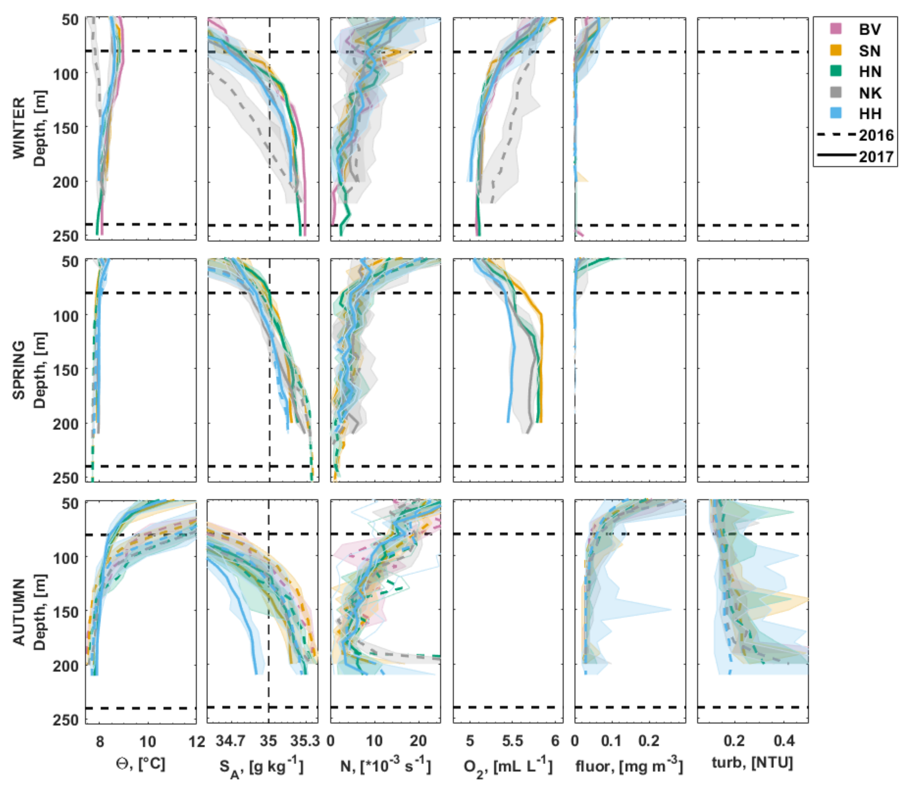
3.2.1. Water Column Hydrography

Waters in Langenuen consisted of seasonally forced surface waters down to ~100 m. The Norwegian coastal water (NCW) and the North Atlantic water (NAW, SA > 35 g kg−1) were present beneath the surface waters (Figure 2). The temperature at water depths above the CWC reefs (<80 m) ranged between 5.3 and 16.3 °C with the cool temperatures (<8 °C) recorded in winter (January 2017 and February 2016) and spring (April 2017 and May 2016) and the warm (>9 °C) temperatures observed in autumn (August 2017 and October 2016). Waters with temperatures >12 °C reached the depths of the uppermost corals (>80 m) at the three southernmost sites (HH, NK, and HN) in October 2016. The thermocline depth varied from 30 m in April 2017 to 100 m in October 2016. Beneath 80 m, the annual temperature range was between 7.5 and 12.2 °C, with a mean temperature of ~8 °C at CWCs living depths. Opposite to the surface waters, the cool bottom water temperatures (<7.8 °C, at depths >200 m) were measured in May 2016, August 2017, and October 2016, while the warm bottom temperatures (>8 °C, at depths >200 m) were recorded in January 2017, February 2016, and April 2017 (Figure 2, Table 3).
Above 80 m, salinity varied from <30 g kg−1 at the surface (<20 m) to close to 35 g kg−1 at depths ~80 m. The halocline depth varied from 20 to 60 m (not shown) except in February 2016, when the water column was well mixed (Figure 2). The 35 g kg−1 isohaline depth (indicating North Atlantic water) varied from 220 m at the HH reef located south of the Langenuen in August 2017 to 75 m at the SN in April 2017. At the depths where CWCs occur, the salinity varied from <34.5 g kg−1 at wall settings at depths 80–110 in February 2016 and in autumn to >35.3 g kg−1 at depths >180 m in May 2016 and at depths >140 m in August 2017 (Figure 2, Table 3). In general, the northern sites were saltier than the southern sites indicating the NAW route from Korsfjord and fresh water output from Hardangerfjord. The surface layer (<80 m) was well stratified (N > 7 × 10³ s−1) throughout the year. The strongest stratification occurred in May and August 2017 and in October 2016. Beneath 80 m, stratification varied from 0.2 to 20 × 103 s−1 (Figure 2) without a clear seasonal or latitudinal signal. The waters at the CWC living depths were less dense at shallower wall reefs (HH, SN) than deeper bank and wall settings (NK, BV, HN) (Table 3). Sigma-theta values >27.35 kg m−3 were measured at all sites in May 2016, August 2017, and October 2016 (Table 3). Across the water column and seasons, dissolved oxygen ranged from 4.96 to 7.11 mL L−1. In winter (January 2017 and February 2016), oxygen decreased with depth, and in April 2017, oxygen increased from 50 to 100 m and was well mixed beneath 100 m (Figure 2). At CWC living depths, oxygen ranged from 4.96 to 5.81 mL L−1. Fluorescence reached values >1 mg m−3 in the uppermost 20 m in April 2017 and in October 2016 (not shown). Beneath 50 m, the fluorescence values were <0.05 mg m−3 (Figure 2). In October 2016, turbidity reached values >1 NTU at the surface and at the bottom. The mean turbidity through the water column was ~0.2 NTU (Figure 2).

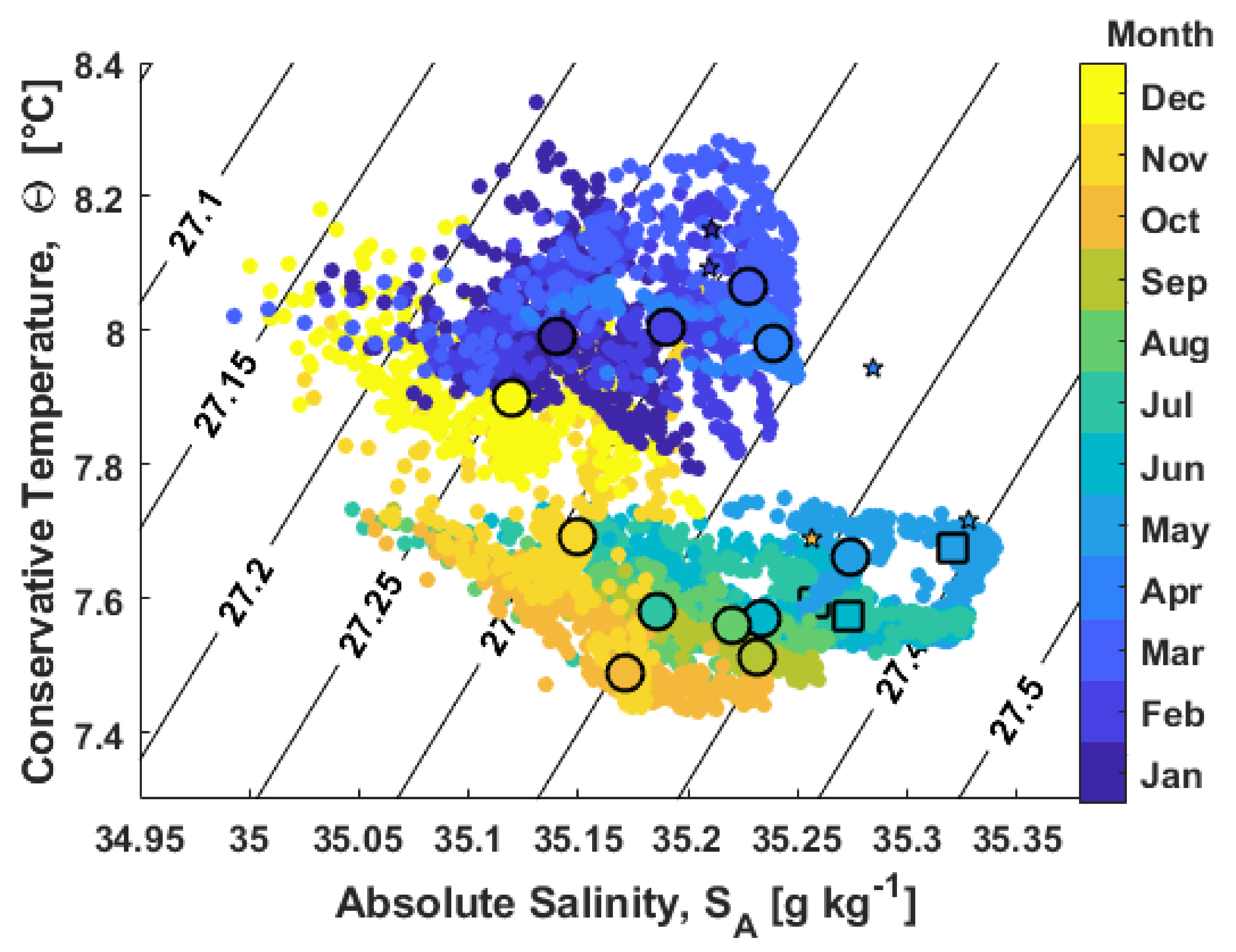
3.2.2. Bottom Water Hydrography

The annual bottom temperature at Nakken bank reef ranged from 7.4 to 8.3 °C, with a mean temperature of 7.8 °C. This included two distinct phases: cool temperatures (<7.8 °C) observed from May to mid-November and warm temperatures (>7.8 °C) measured from late November to April (Figure 3), indicating heat dissipation from the surface during autumn and water column mixing in spring. March was the warmest month. September and October were the coolest months (Figure 3 and Figure 4). Bottom water salinity varied between 35.00 and 35.34 g kg−1 with the lowest salinities (<35.2 g kg−1) observed in autumn and winter, and the highest salinities observed in late spring, indicating the water source variability between North Atlantic water (SA > 35 g kg−1)-dominated and Norwegian coastal water-dominated waters. The salinities measured by MLM were ~0.05 g kg−1 higher than those measured by SLM (Figure 3) during the time both landers were at the sea bed, whereas measured temperatures were similar. Relatively high sigma-theta (density) values of >27.35 kg m−3 were measured from May until October (Figure 3). Bottom water oxygen values varied from 6.58 to 6.68 mL L−1, with the highest values in October and lowest values in January (Figure 4) following temperature variations. Turbidity values reached up to 1.5 NTU between July and August. Turbidity values dropped in October to around 0.15 NTU. They remained low (<0.15 NTU) with few turbid events (>0.2 NTU) until the end of the deployment (Figure 4).

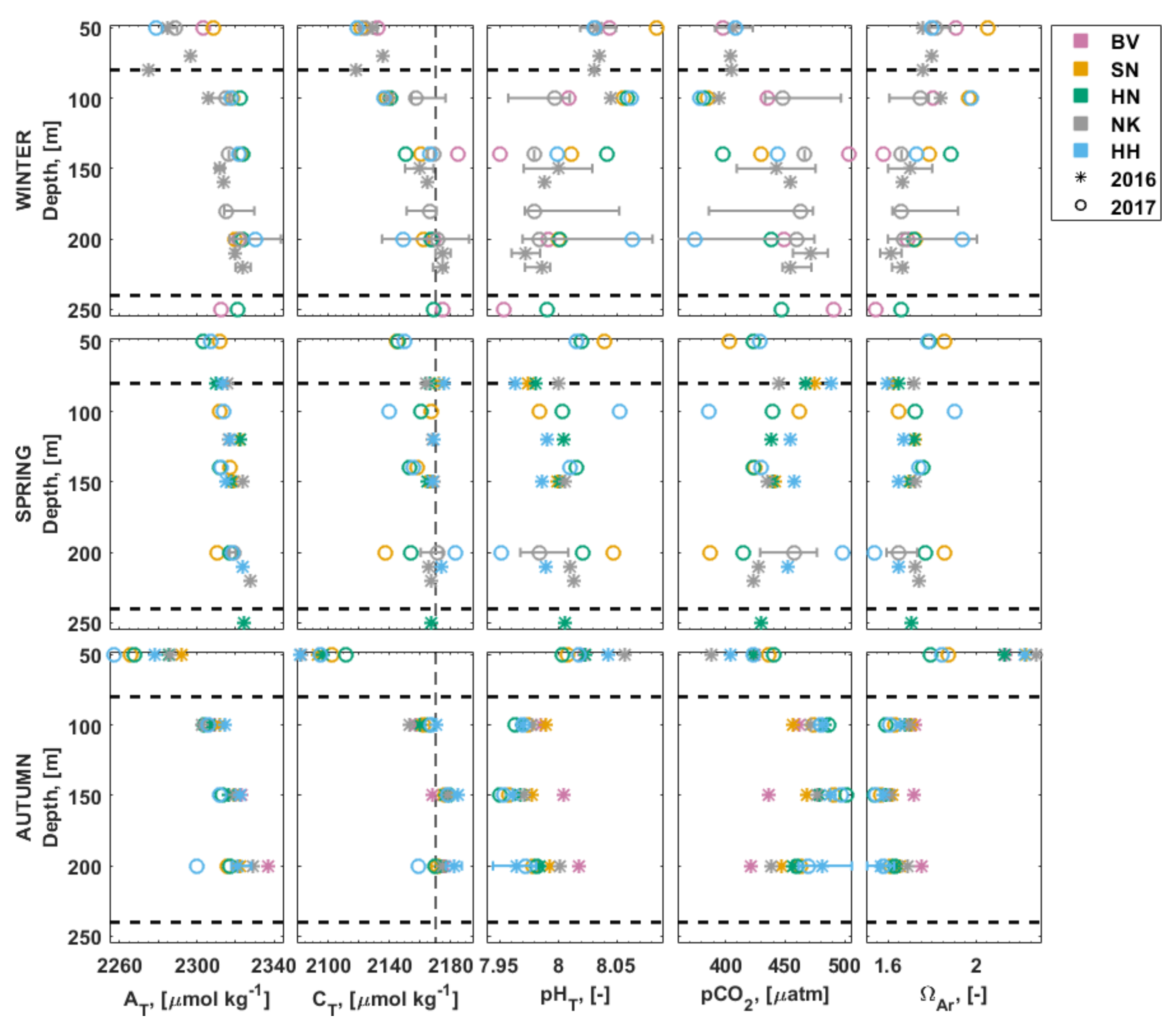
3.3. Carbonate Chemistry in the Water Column

Concentrations of dissolved inorganic carbon (CT) and total alkalinity (AT) increased with depth at all sites and times. Below 50 m (Figure 5), the variability between the sites was largest in winter (February 2016 and January 2017) and smallest in autumn (August 2016 and October 2017). Variability was higher at 200 m than at intermediate depths of 100–150 m. Relatively low surface values (AT < 2100 µmol kg−1 and CT < 2000 µmol kg−1) occurred in autumn (August 2017 and October 2016) (Table 3). Both the lowest (CT = 2135 µmol kg−1) and the highest (CT = 2192 µmol kg−1) CT values at CWC living depths were measured at the NK bank reef at 200 m depth during the 16 h sampling period in January 2017. The highest AT value (2343 µmol kg−1) was also measured during the same period and place. The lowest AT of 2300 µmol kg−1 was measured at HH wall reef at 200 m depth in August 2017. In general, the northernmost sites (BV and SN) had higher AT in autumn and higher CT in winter and autumn at 200 m depth than sites farther north, but short-term variability recorded over tidal cycle at a single location (HH or NK) was larger than this between sites difference.
pHT ranged from 7.94 to 8.08 throughout the water column over the study period (Figure 5, Table 3). Low values (<7.98) were measured at depths >140 m at BV bank reef and at depths >100 m at NK bank reef in winter (January 2017 and February 2016), at ~80 m depth at wall reefs HH and SN in May 2016, at ~200 m depth at HH and NK in April 2017 and at depths >100 m at all sites except BV in autumn with a minimum at 150 m depth. High values of >8.03 were measured at the surface (<40 m) at all sites and times (Table 3). Below 80 m, high values (>8.03) were measured at HH at ~100 m and at NK at ~ 200 m depth in winter (January 2017 and February 2016) and in April 2017. The pCO2 ranged from 293 to 452 µatm above 80 m. Beneath 80 m, it ranged from 356 µatm at ~200 m at NK in January 2017 to 506 µatm at ~200 m at HH in October 2016 (Figure 5, Table 3). Above 80 m, ΩAr ranged from 1.41 at NK in January 2017 to 2.28 at NK in August 2017, and below 80 m, it ranged from 1.50 at ~200 m at HH in October 2016 to 2.00 at ~200 m at NK in January 2017. ΩAr and ΩCa had maxima at the surface in autumn (August 2017 and October 2016) (ΩAr > 2.1 and ΩCa > 3.3). The low (ΩAr < 1.59) aragonite saturation levels were measured at 150–200 m depths at wall reefs (HH, SN, HN) in autumn (August 2017 and October 2016), at ~200 m at HH in April 2017, and at depths >140 m at BV in January 2017 (Figure 5, Table 3).
Carbonate chemistry sampling was performed over several hours at two stations at two different times: At wall reef HH (corals at depths 80–220) in October 2016 and at bank reef NK (corals at depths 190–220) in January 2017. During a 26 h sampling period at 200 m depth at the HH wall reef in October 2016, Θ and SA were relatively stable with ranges of ∆Θ = 0.14 °C and ∆SA = 0.11 g kg−1 (Figure 6). Over the sampling period, the carbonate system parameters changed by: ∆AT = 10 µmol kg−1, ∆CT = 10 µmol kg−1, ∆pHT = 0.032, ∆pCO2 = 45 µatm, ∆ΩAr = 0.12, and ∆ΩCa = 0.19. This is comparable to the seasonal variability between winter and summer from single measurements at HH at this depth ∆AT = 11 µmol kg−1, ∆CT = 34 µmol kg−1, ∆pHT = 0.112, ∆pCO2 = 123.6 µatm and ∆ΩAr = 0.4 (Figure 6). The flow direction at nearby Nakken reef was southward with speeds between 4 and 43 cm s−1.
Short-term temporal variability of carbonate parameters at Nakken bank reef in January 2017 was larger than the short-term variability at Huglhammaren in October 2016. During this sampling period of 16 h, Θ and SA at 200 m varied from warm (Θ >8 °C) and less saline (SA < 35.23 g kg−1) conditions to cool and saltier conditions and back. The overall ranges were ∆Θ = 0.32 °C and ∆SA = 0.05 g kg−1 (Figure 6). The carbonate chemistry followed the changes in flow direction with high CT and low AT values observed with northward flow (=warm and fresh phase). The highest AT value (2343 µmol kg−1) was also measured during northward flow conditions. Over the sampling period, the carbonate system parameters showed large ranges of: ∆AT = 26 µmol kg−1, ∆CT = 57 µmol kg−1, ∆pHT = 0.11, ∆pCO2 = 118 µatm, ∆ΩAr = 0.41, and ∆ΩCa = 0.64. This is larger than the seasonal variability between spring and summer from single measurements at NK at this depth ∆AT = 10 µmol kg−1, ∆CT = 41 µmol kg−1, ∆pHT = 0.04, ∆pCO2 = 47.6 µatm, and ∆ΩAr = 0.14 (Figure 6).

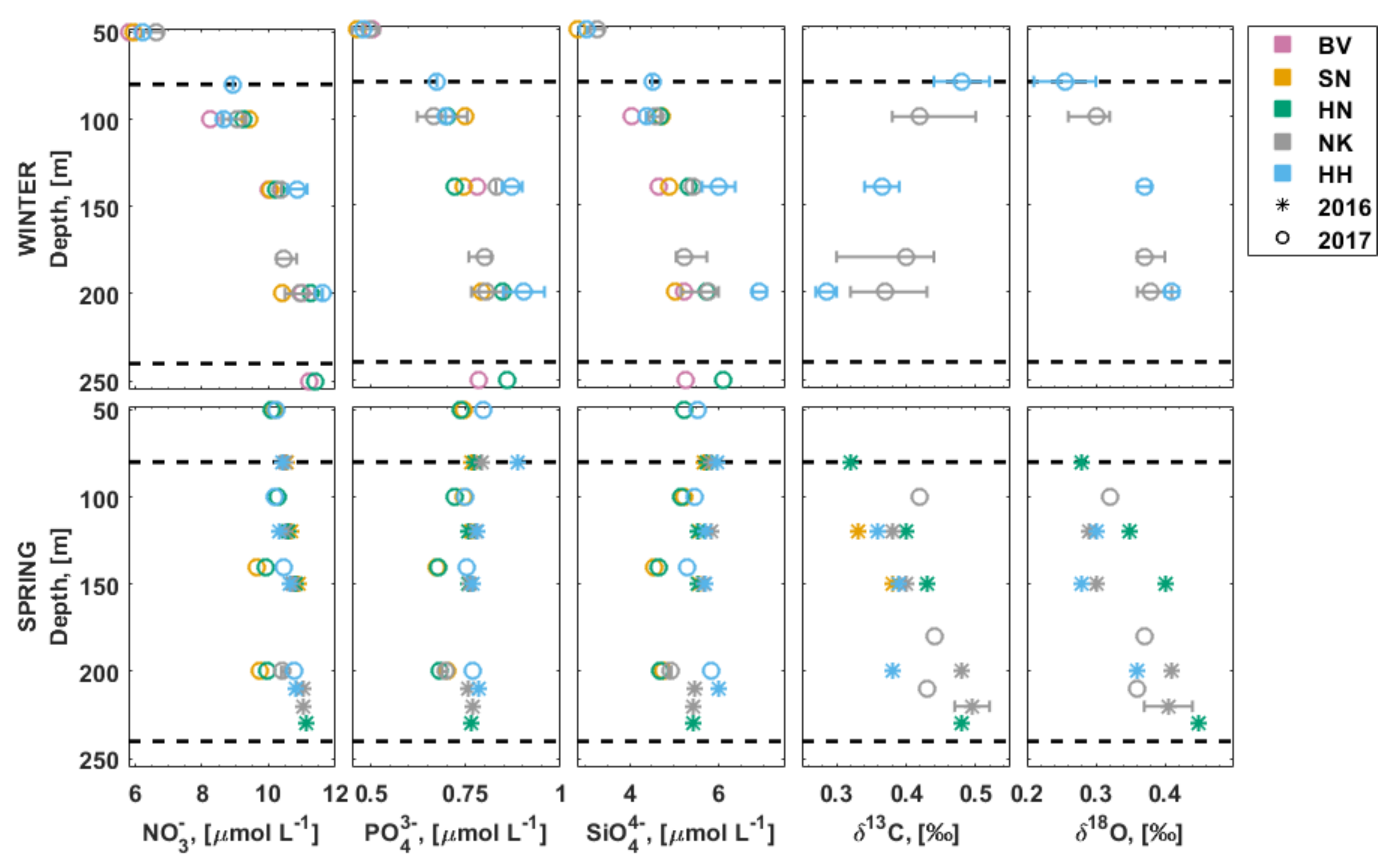
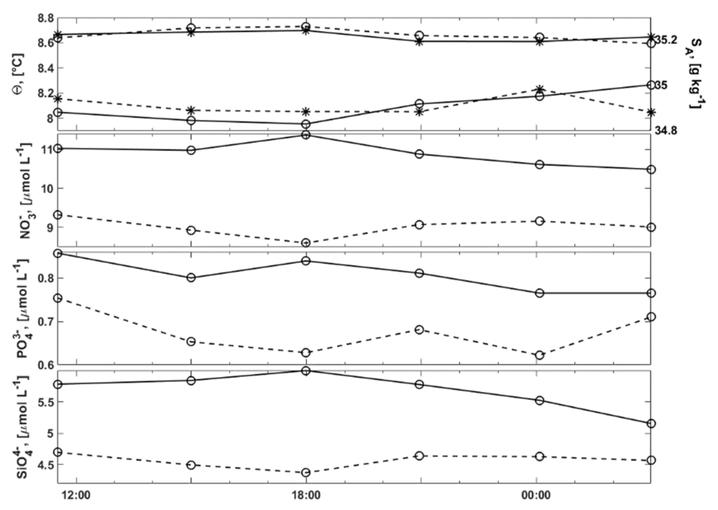
3.4. Inorganic Nutrients in the Water Column

Within the uppermost 80 m, nitrite (NO2) and ammonium (NH4+) concentrations ranged from 0.064 to 0.175 µmol L−1 and from 0.075 to 1.04 µmol L−1, respectively, with the highest concentrations measured in May 2016 (not shown). Below 80 m, their concentrations were too low (<0.06 µmol L−1) for reliable measurements.
Nitrate (NO3), phosphate (PO43−), and silicate (SiO44−) concentrations all increased with depth in January 2017. In spring (May 2016 and April 2017), the concentrations were mixed beneath 80 m (Table 3, Figure 7). In January 2017 and April 2017, nutrient concentrations were higher at the southernmost (HH and NK) sites at depths >100 m than at sites farther north. In January 2017, the surface (<40 m) nutrient concentrations (<6.65, <0.51, and <3.26 µmol L−1) were higher than during spring (May 2016 and April 2017) (<5.13, <0.4, and <2.68 µmol L−1) (Table 3). Beneath 80 m, both the highest and the lowest nutrient concentrations were measured in January 2017. The highest concentrations were measured at ~200 m depth at HH and the lowest at ~100 m depth at BV, HH, and NK. At CWC living depths, nutrient concentrations at the shallow wall (HH and SN) and deeper bank (NK and BV) reefs were on average for NO3 ~10.34 and ~10.80 µmol L−1, for PO43− ~0.78 and ~0.77 µmol L−1, and for SiO44− ~5.48 and ~5.41 µmol L−1, respectively (Table 3).
At Nakken, CTD data and nutrient samples were collected from 100 to 200 m depth every three hours for 16 h between January 3–4, 2017 (Figure 8). The hydrographic range at 200 m is presented in Section 3.3. At 100 m depth, the variation patterns in Θ and SA differed from 200 m. They varied from cool (Θ < 8.7 °C) and saltier (SA > 34.9 g kg−1) conditions to warm and less saline and back. The overall ranges were ∆Θ = 0.14 °C and ∆SA = 0.10 g kg−1 (Figure 8). The range of concentrations at 200 m and 100 m depth over the sampling period reached ∆NO3 0.88 and 0.73 µmol L−1, for ∆PO43− 0.09 and 0.13 µmol L−1, and for ∆SiO44− 0.84 and 0.32 µmol L−1, respectively. As for the carbonate system parameters, the change from low nutrient concentrations and low-temperature conditions to higher nutrient concentrations and warmer temperatures at 200 m depth coincided with flow velocity shift from strong southward velocity to low northward velocity (Figure 6 and Figure 8).

3.5. Stable Isotopes

The distribution of δ13C within the water column varied between the different sampling times (Figure 7). In January 2017, δ13C decreased with depth. In April 2017, the water column was well mixed with respect to δ13C, and in May 2016, δ13C increased with depth. The δ13C value was generally higher at bank reefs (0.41‰ ± 0.06‰, depths 190–220 m) than at shallower wall reefs (0.37‰ ± 0.07‰, depths 80–220 m) (Table 3). δ18O increased with depth and had similar ranges for all sampling times. Therefore, δ18O was higher at bank reefs (0.39‰ ± 0.03‰) than at shallower wall reefs (0.34‰ ± 0.06‰) (Table 3). In May 2016, when samples were taken from most of the sites, δ18O had the largest range at ~150 m depth of Δδ18O = 0.12 ‰ (Figure 7). With a relatively low sample size (n = 37), these results are preliminary and only provide us the first look at the distribution of stable isotopes in Langenuen. Thus, these results have to be confirmed by future research.

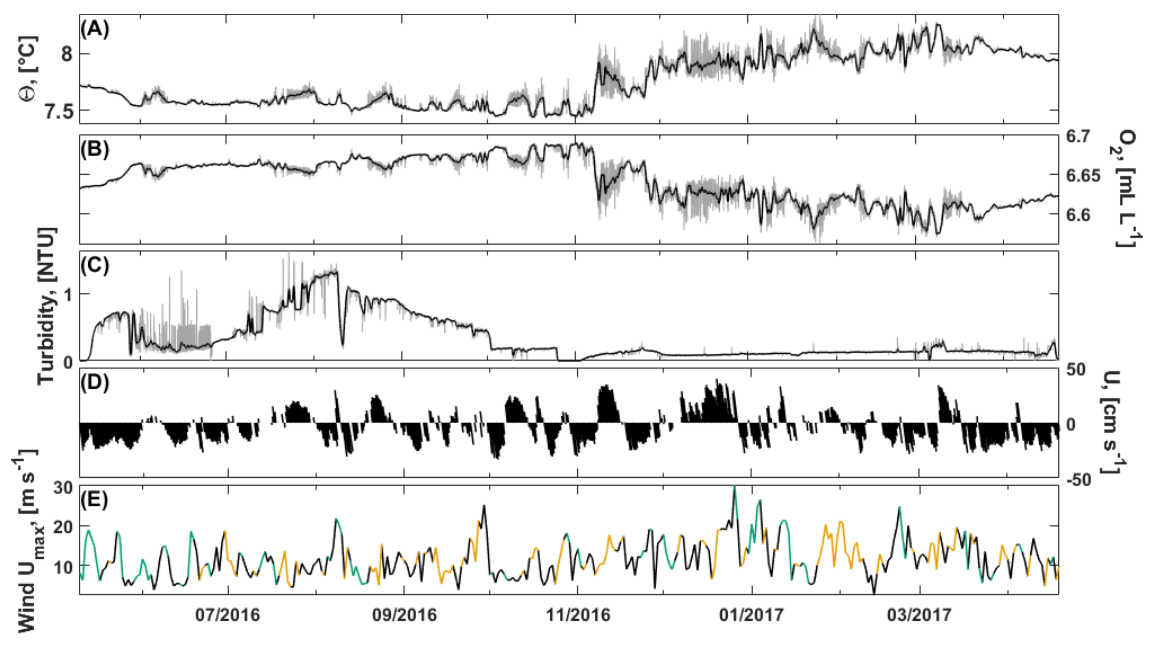
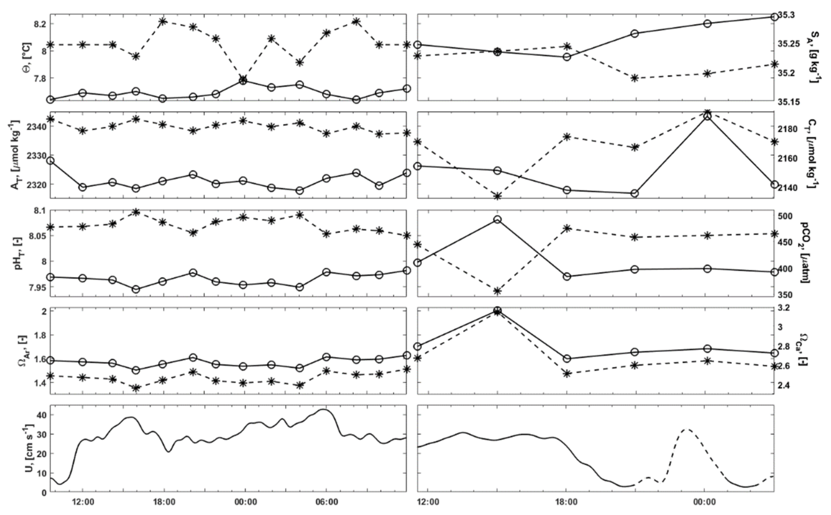
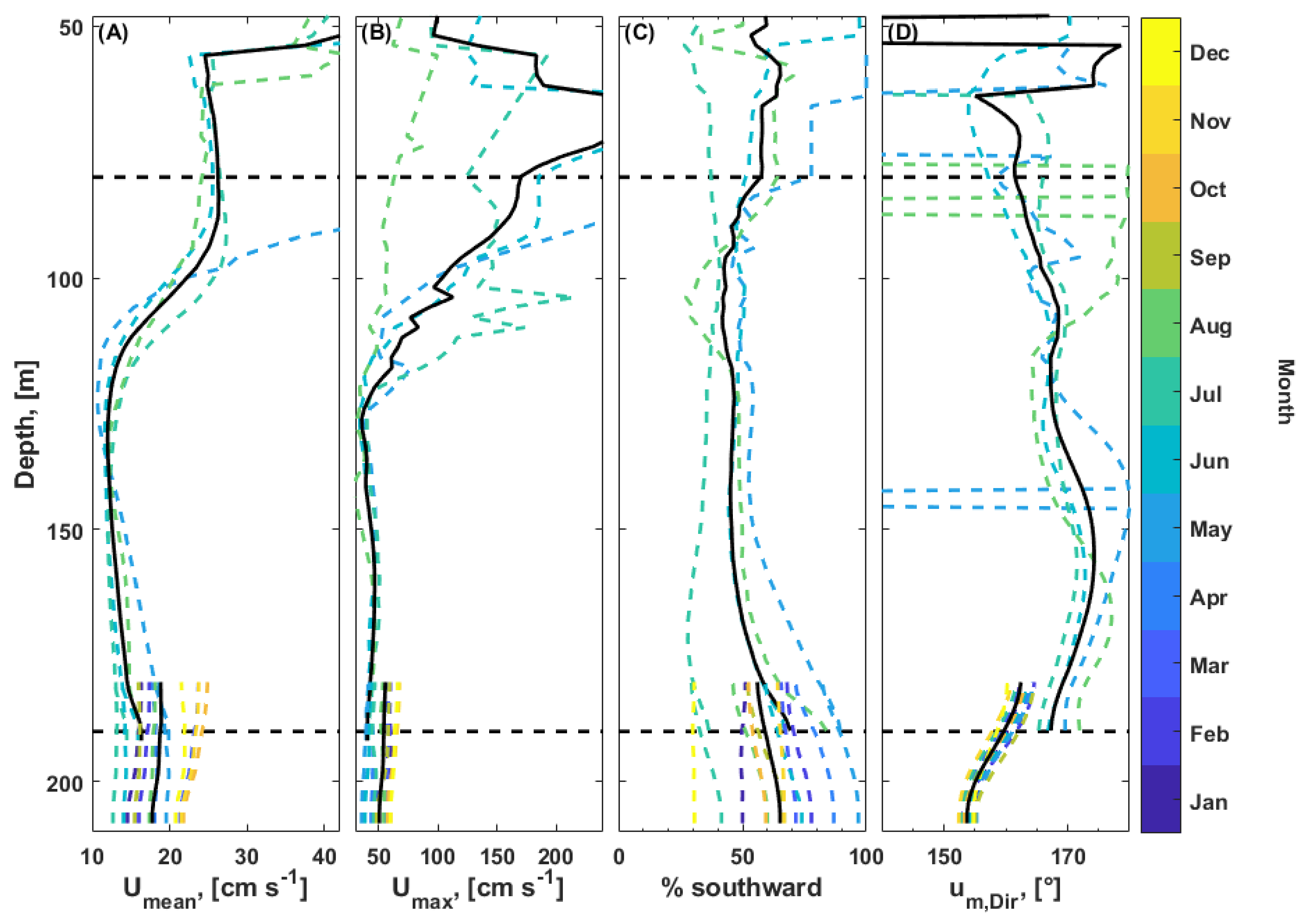
3.6. Current Measurements

3.6.1. Flow Regime

The flow below 180 m was strong (mean 18 cm s−1, max 60 cm s−1) with a semidiurnal tidal component (Figure 4 and Figure 9, Table 3). The monthly mean flow speed (Umean) varied between 12 and 25 cm s−1. Low mean flow speeds (Umean < 15 cm s−1) were measured in June and July, and high mean flow speeds (Umean > 20 cm s−1) were measured in March and in late autumn in between October and December. During the remaining months, Umean varied between 16 and 18 cm s−1. At depths above 180 m (recorded with MLM), flow speeds varied more. From May to August, Umean was < 15 cm s−1 in between 115 and 180 m depth. Umean reached maxima at 90 m and at <50 mm depth with 27 and >45 cm s−1, respectively (Figure 9A).
The maximum monthly flow speeds (Umax) below 180 m depth varied between 30 and 70 cm s−1. Umax was <45 cm s−1 in May and June and ~60 cm s−1 between October and December. During the other months, Umax varied between 50 and 55 cm s−1. Between 125 and 180 m water depth, Umax was <50 cm s−1. At depths of <117 m, Umax was >100 cm s−1 except in August, with peak speeds (>200 cm s−1) measured around 60 and 100 m depths (Figure 9B).
The current direction was determined by the orientation of the fjord and was dominantly southward (between 90° and 270°) beneath 180 m, varying in between 80 and 180 m, and southward (May and June) or northward (July and August) near the surface (Figure 9C, Table 3). In July and December, the flow direction was dominantly northward (Figure 9C). The direction of the most energetic flow, um, was dominantly southward across the water column (150°–163°, at depths >180–208 m and 160°–170° at depths <180 m). The northward flow was measured at ~150 m depth in May and depths <100 m in August (Figure 9D).
The flow regime at NK bank reef was mostly subcritical, but it supported hydraulic jumps with flow velocities >Umean. These are observed as rapid changes in hydrographic parameters. For example, in the winter months, temperature, salinity, and turbidity fluctuated within 12 h ∆Θ = 0.4 °C, ∆SA = 0.15 g kg−1, and ∆turbidity >0.2 NTU. Following the categorization of Juva et al. (2020) [22], the flow state is thus partially subcritical (PBsc).

3.6.2. Tides

Tidal analysis of the pressure data explained 87.2% and 95.6% of the pressure fluctuations with 28 and 22 significant constituents at SLM and MLM, respectively. At both lander sites, the semidiurnal (M2) signal generated the largest amplitude of 0.34 dbar. The other significant constituents were diurnal, semidiurnal, and higher frequency constituents (Table 4).
The analyses of the tidal constituents from the near bottom horizontal velocity records revealed a different picture with more significant higher frequency harmonics than in pressure. With 14 and 12 significant tidal constituents, tidal analysis explained 7.2% and 14.1% of the horizontal bottom velocity fluctuations at SLM and MLM, respectively. The M2 generated amplitudes of ~5 cm s−1 with flow direction to NNW (330°–341°), the opposite of the mean flow direction (Table 4).

4. Discussion

In this study, we investigated the dynamics of the flow and environmental (hydrography, carbonate chemistry, and inorganic nutrients) conditions around three L. pertusa-dominated wall reefs and two bank reefs in a narrow fjord on diurnal, seasonal, and annual time scales. Our results suggest that both hydrodynamics and hydro-biogeochemistry regulate the distribution and health of the reefs in Langenuen and that the fjord is likely to be in a state of change that has been ongoing since the 1980s.

4.1. Flow Dynamics

All five CWC reefs are healthy, but their limited spatial extent suggests that areas with suitable living conditions for CWCs are narrow both vertically and horizontally. CWC occurrences, both on the walls and banks coincide with the most dynamical parts of the fjord.
The flow regime in Langenuen is controlled by the Norwegian coastal current and modified by bathymetry, wind conditions, and tidal forcing [83,84,85,86]. In the upper 100 m, the flow is strong with peak speeds of >100 cm s−1. At L. pertusa living depths (100–220 m), water flow is predominantly southward with mean speeds of <20 cm s−1 and peak speeds of ~60 cm s−1 (Figure 9). This is comparable to other CWC sites in the NE Atlantic [27,31,87]. The flow down to ~120 m is driven by southerly winds and Norwegian coastal water entering the fjord above the sill depth from the south [88,89]. Flow in deeper water layers is driven by seasonal density differences outside the fjord system. For example, the flow is reversed to northward-dominated at 120–200 m depth in December and in January (Figure 9C), when prevailing northerly winds (Figure 4D) [90,91] create coastal upwelling that pushes warm and deep North Atlantic water over the sill and into the deep fjord basin [92]. Intrusions of high salinity and relatively warm North Atlantic water renew the basin water in the fjords [89,93] and maintain aerobic conditions at the bottom [94]. At Nakken, the tidal flow was small compared to the residual flow (~5 vs. ~20 cm s−1). This is common in these coastal waters [95,96]. Similar amplitudes have been recorded in Hardangerfjord, the main fjord to which Langenuen is a tributary [93].
In the Langenuen Fjord system, the distribution of CWC reefs, both on walls and banks, seems to be governed by small-scale hydrodynamics. At the wall reefs of HH and SN, L. pertusa corals live just beneath the seasonal thermocline and the fastest flow layer (>100 m). The upper vertical limit of the corals could be set by this fast flow layer as in strong currents, the polyps could bend backward, reducing the feeding surface [97], and prey could escape from the polyps [98], restricting energy uptake in the coral. The 100 m depth also coincides with the strongly stratified layer in late summer and autumn (N > 20 × 10−3 s−1, Figure 2), which could reduce the zooplankton migration to CWC living depths [99,100]. Below 100 m, flow is slower, and the framework of the CWCs further reduces flow speeds due to friction [28] toward the efficient prey capture speeds of the L. pertusa [34,98]. Moreover, the CWC framework acts as a natural sediment trap allowing the corals to capture and use the enhanced particle delivery. At these depths, thriving colonies of L. pertusa and M. oculata occur on the vertical walls. The lower vertical distribution limit of the CWC growth on vertical walls is created by the lack of hard bottom substrate when moving beneath 200 m depth at Straumsneset and Huglhammaren and below 240 m depth at Hornaneset.
At the bank reefs, the topography-flow interaction is suggested to directly influence the health and growth of CWCs [22]. At the Nakken bank reef, the flow supports periodic hydraulic jumps at high flow speeds. This will create a link between the surface and the deep reefs. During these turbulent events, resuspended organic particles that have settled to the sea bed would locally elevate food supply to the reefs compared to the surrounding deep sea-bed. These processes could be particularly important during periods of food limitation [101]. However, during the periods of periodic hydraulic jumps also mineral particles will be resuspended and settled. It is assumed that patchy reefs with similar flow regimes would have high vertical growth rates to prevent burial [22]. Maier et al. (2020) [101] estimated the linear growth at NK to be 13 mm year−1 for new polyps. This is 30% to 100% higher than the linear growth measured for other Norwegian reefs located farther north [102,103]. These areas occur likely in a more dynamic flow state preventing the settling of particles and keeping the reef clear from heavy sedimentation. This would reduce the need for large vertical growth while increasing the need for horizontal growth and bridging between polyps, enforcing the coral skeleton to withstand high physical forcing without breaking [22]. At the Nakken bank reef, turbulent conditions created by hydraulic jumps are only present in winter, i.e., from October to December (Umean >20 cm s−1, and Umax >50 cm s−1, Figure 9). It is plausible that the emergence and growth of new polyps, taking place at this particular reef from December to March [101], is initiated by the increased sedimentation caused by the periodic hydraulic jumps. Growth rates 60% higher than those measured at NK have been documented for L. pertusa in the Gulf of Mexico, where corals form similar patches as observed in NK [104].

4.2. Hydrographic and Biogeochemical Conditions

Seasonal signals in hydrography and biogeochemistry in the Langenuen Fjord are strong, similar to the general area [92]. All CWC reefs in Langenuen occur in well-oxygenated (O2 > 4.9 mL L−1) and inorganic carbon-rich (CT > 2135 µmol kg−1) waters. The hydrographic (Θ and SA), alkalinity (AT), and inorganic nutrient (NO3, PO43−, and SiO44−) ranges are within previously reported values from NE Atlantic CWC sites (Table 5) [11,13,29,39,53].
Due to surface warming in spring and summer, the seasonal isopycnal reaches ~100 m. The uppermost CWCs on the wall reef setting (at 80–100 m, HH) experience temperatures >12 °C in late summer before the water is mixed in late autumn. This is ~4 °C warmer than the mean temperature at these shallow reefs and likely enhances the metabolism of L. pertusa and increases their energetic demand [36,41]. Together with strong flow speeds (limiting prey capture rates in L. pertusa), seasonal high temperatures could restrict the upper limit of the CWCs on the fjord wall. Beneath the seasonal warming layer of 100 m, annual ranges of hydrographic variables were small (∆Θ = 1.92 °C, ∆SA = 0.96 g kg−1) particularly when compared to the largest measured temperature fluctuation at any CWC site, namely the ~9 °C (5.8–15.2 °C) temperature fluctuation within a day registered in the Cape Lookout area, NW Atlantic [105]. Bottom temperatures decrease in late winter due to dissipation from the surface and remain low throughout summer due to the pronounced water column stratification established by the spring freshwater flood [106]. Due to relatively warm winter temperatures in the deeper layer and the freshwater influence, reefs occur in less dense waters than suggested for healthy CWC sites in NE Atlantic (i.e., σΘ = 27.35–27.65 kg m−3, [12]).
At Langenuen, the dissolved inorganic carbon was at times high, and a maximum value of 2192 µmol kg−1 was observed. This is higher compared to what is previously linked to thriving NE Atlantic CWC occurrences (CT < 2170 µmol kg−1, [15]). On the other hand, total alkalinity (2300–2343 µmol kg−1) was similar to other NE Atlantic CWC sites (2287–2377 µmol kg−1, Table 5). For comparison, the typical carbonate chemistry properties in Atlantic core water in the Norwegian Sea is about 2160 µmol kg−1 and 2310 µmol kg−1 for CT and AT, respectively [107]. Regional studies of carbonate chemistry surrounding CWC ecosystems in the Gulf of Mexico [14], Gulf of Cadiz [15], Mauretania [15], Mediterranean [10,15], and Marmara Sea [10] have shown that CT > 2170 µmol kg−1 is common for CWC sites outside the NE Atlantic (Table 5) while significantly higher (AT > 2500 µmol kg−1) alkalinity levels are measured only at the Mediterranean and the Marmara Sea CWC sites. Together with regional hydrographic (Θ, SA) conditions, the relatively high AT result that the aragonite saturation is also relatively high (ΩAr > 2.5) in the Mediterranean CWC sites compared to other basins, where values <2.0 are common (Table 5). Consequently, this study emphasizes the importance of estimating both CT and AT since it is the relationship between them that determines the CaCO3 saturation. These regional ranges are obtained from single time point measurements that do not include the variability on the diurnal level.
Table 5. The range (published min–max) of environmental conditions at different regions, specifically at the depth and site of known Lophelia pertusa, Madreora oculata, or Desmophyllum dianthus occurrences, comparing data from this study with data available in the literature. Abbreviations: GoC: Gulf of Cadiz, Ma: Mauretania, Me: Mediterranean, GoM: Gulf of Mexico, CF: Chilean Fjords, MS: Marmara Sea, TS: Tassman Seamount, C-Refs.: References for carbon system data, N-Refs.: References for nutrient data, nd: no data reported, * Only mean salinity reported in [108].
LocationThis StudyNE AtlanticGoCMaMeGoMCFMSTS
Depth, (m)80–220100–1000606–1322451–568200–850307–62020–2009321050
Temperature, (°C)7.4–12.25.9–10.69.2–11.09.7–11.712.8–14.0nd10.6–12.514.54.59
Salinity, (-)33.93–35.3935.0–35.735.6–36.035.2–35.438.6–38.835.05 *31.7–33.038.834.4
AT,
(µmol kg−1)
2300–23432287–23772332–23422314–23752577–27422259–23912136–223526102315
CT,
(µmol kg−1)
2135–21922088–21862180–22002183–22402307–23332135–22312025–218824702218
ΩAr, (–)1.50–2.011.35–3.031.43–1.831.31–1.582.59–4.061.19–1.690.78–1.601.461.02
C-refs. [15,53][15][15][10,15,108][108][10,109][10][10]
PO43−,
(µmol L−1)
0.67–0.960.4–1.6 0.20–0.41
NO3,
(µmol L−1)
8.64–11.614.1–23.4 nd
NH4+,
(µmol L−1)
<0.60.5–1.6 0–0.29
SiO44−,
(µmol L−1)
4.37–6.922.1–46.6 nd
N.-Refs. [11,53] [108]
The short-term variability in carbonate chemistry in Langenuen is large, and the highest values are linked to the tidal cycle. Similarly, high CT concentrations have been observed in dynamical NE Atlantic CWC mounds in the southern Rockall Bank [53]. There, values up to 2186 µmol kg−1 were measured over a tidal cycle, indicating that L. pertusa is resilient to CT levels exceeding 2170 µmol kg−1, at least over short time scales. At Rockall Bank, the tidal range of CT was 58 µmol kg−1. This is similar to short-term (within 16-h) variability measured at NK reef (ΔCT ≈ 57 µmol kg−1) in January 2017 and to the annual ranges of CT at CWC living depths at other Langenuen reefs (ΔCT ≈ 51 µmol kg−1 at HH, and ΔCT ≈ 39 µmol kg−1 at SN). The short-term changes in carbonate chemistry at Langenuen reefs cannot be explained by salinity and temperature changes alone. For example, the pCO2 change is about 4.2% per 1 °C, implying that the temperature effect on pCO2 could explain ~5 µatm of the 124 µatm difference recorded at Nakken reef during 16 h in January 2017. This large variability is most likely caused by rapid change in the dominant water mass from Norwegian coastal water to North Atlantic water. NAW has high pCO2, thus large CT, but also relatively high AT. Therefore, pHT and ΩAr are generally higher in NAW than in waters containing freshwater (such as NCW), and large changes in the whole carbonate chemistry are possible during short time periods. It is also plausible that the presence of North Atlantic water with higher ΩAr compared to Norwegian coastal water is buffering ocean acidification in Langenuen, and strengthening of the coastal stratification outside the fjord system caused by warming could reduce its presence at the Langenuen coral reefs in the future.
Observed differences between the five reefs were not consistent between the different time periods or seasons sampled. This variability is at least partly a consequence of the short-term variability that is not captured with single time point measurements or replicates taken close to each other in time. The observed variability over the 16 h sampling period in January 2017 was larger both between the sites and at NK compared to other months. The high fluctuation in winter could be caused by a combination of the storm event and dynamical winter conditions (i.e., weaker stratification, stronger flow, water source variation between the north (Korsfjorden) and south (~Utsira) more than during other seasons), see Figure 2, Figure 4, Figure 6 and Figure 9. This kind of extreme event is likely to occur each year, and based on meteorological reports [90,91], it is likely that even more energetic events occurred in winter 2016–2017. Since the tidal component causes large variability in the carbonate chemistry, the full seasonal and diurnal variability of the carbonate and nutrient chemistry should be measured in further ocean acidification studies [48].

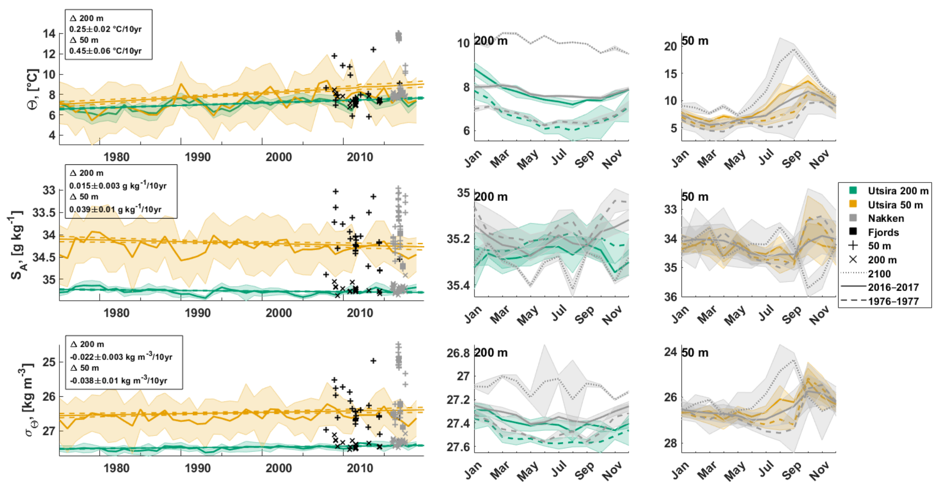
4.3. Long-Term Changes

The measured time period (from February 2016 to August 2017) is not long enough to fully capture the interannual variability nor the long-term trends of environmental conditions occurring in the Langenuen Fjord. However, because of the water exchange between Langenuen and the open ocean above sill depth, the mean hydrographic conditions at Langenuen CWC depths can be correlated to the fixed coastal station Utsira south of Langenuen (Figure 1A and Figure 10) [110]. Sætre et al. (2003) [38] reported that both temperature and salinity decreased between 1950 and 1989 along the Norwegian coast. At Utsira, the winter temperature (JFM) decreased from 7.6 to 7.0 °C and salinity from 35 to 34.8 [38] at 150 m depth during this period. These trends are affected by basin-wide phenomena such as “great salinity anomalies” (GSAs) [111,112,113] and the North Atlantic oscillation (NAO) [114]. GSAs are low-salinity/low-temperature events that are formed by cold winters, freshwater outflow, strong northerly winds, and a large sea ice extent in the northwestern Atlantic [112]. A positive NAO index is associated with mild winters, an increase in westerly winds, higher winter precipitation over Scandinavia, and a deeper Norwegian coastal current. GSA salinity minima are reported at Utsira coastal station in 1977–1978, 1987–1989, and 1994–1996 [38]. High temperatures and salinities in between these periods are caused by an increase in the Atlantic inflow combined with the atmospheric conditions associated with periods of positive NAO and a general rise in temperature over the past decades [115]. The decadal forcing acts together with climate change to determine the past, the present, and the future deep-water hydrography within the region and at Langenuen. The whole water column had warmed after the GSA in the 1980s when only salinity returned to previous levels (Figure 10), indicating ocean warming. At Utsira, the increase has been 0.45 and 0.25 °C per decade at 50 and 200 m depths, respectively, since 1975 (Figure 10). If we assume a similar warming trend in bottom temperature at Langenuen, the waters at CWC living depths were ~1 °C cooler in the 1970s compared to the study period 2016–2017. Furthermore, if these warming rates continue at Langenuen, temperatures could seasonally increase to >18 °C at 50 m depth and >10 °C at 200 m depth (Figure 10). The summer thermocline with temperatures >12 °C would reach depths >100 m by the year 2100. The warming within the past 40 years has likely already increased the energy demand of CWCs compared to that in the 1970s, with possible effects on coral energy reserves and reproductive output if these are not met by increased food uptake rates [41].
The warming of coastal waters caused by climate change has likely led to a decreased frequency of intrusions of dense, oxygen-rich North Atlantic water with relatively high ΩAr levels and has caused a general oxygen decline in the basin waters of some western Norwegian fjords with shallow sills (i.e., <100 m) [45,116]. Furthermore, warmer water contains less oxygen. In the Masfjorden, north of Bergen, this multidecadal decline corresponds to a loss of 2.0 mL L−1 over 42 years and an associated 1 °C rise in temperature [45]. A similar decline in oxygen has been reported in Byfjorden, off the city of Bergen, with an accompanying shift in benthic communities toward domination of opportunistic benthic species [116]. Given the observed warming in Utsira, oxygen concentrations have likely decreased in Langenuen as well and are likely to decrease even further in the future. Hebbeln et al. (2020) [35] suggested that L. pertusa populations are highly sensitive to low oxygen conditions of 40%–50% lower than the ambient oxygen values. From observed conditions, a decline of 40% from present values would set the lower oxygen limit in Langenuen to ~2.5 mL L−1 compared to the global limit of <1.5 mL L−1 [36,117,118]. If a decline of 0.5 mL L−1 per decade continued linearly in Langenuen, corals would be exposed to hypoxic conditions by the end of the century and to conditions <2.5 mL L−1 by the year 2070.
Besides warming waters and oxygen decline, salinity in the surface layer has been decreasing along the Norwegian coast [38]. At Utsira, the decline at 50 m depth has been up to −0.05 g kg−1 per decade between May and September since 1975 (Figure 10), but salinity has increased slightly during other months and at other depths. This long-term decrease in salinity at the surface is partly caused by increased precipitation and retreat/melting of glaciers, substantially increasing freshwater run-off. Førland and Hanssen-Bauer (2000) [119] demonstrated that precipitation in northern Norway has increased by 1.7% per decade during 1961–1990. Hanssen-Bauer et al. (2003) [120] projected an annual increase of 15% in precipitation from 1980–1999 to 2030–2049 in western Norway. During the last decade, the glaciers of Norway have continuously retreated ([121] and references therein). This could further increase the surface stratification and reduce the surface-bottom interaction during the melt water period.
Driven by warming, the water column has become less dense within the past 40 years in Utsira at a rate of 0.037 kg m−3 per decade at 50 m and ~0.02 kg m−3 per decade at 200 m depth. If density has changed similarly in Langenuen, waters at CWC living depths would have been within the suggested sigma-theta range for thriving CWC sites in the NE Atlantic (>27.35 kg m−3) [12] during the 1970s but are lower than that now. Such changes may be critical because the depth zonation of CWCs on the vertical walls may be related to physical boundary conditions at specific depths that act to concentrate food particles [122], and corals cannot physically move to adjust to that.
Freshwater from rivers, rain, and melting glaciers have been observed to decrease AT and ΩAr substantially and play a large role in increasing ocean acidification in surface waters [123,124]. These waters could reach the coral depths during autumn and winter mixing even though the summer stratification is likely getting stronger. Therefore, there is a weak positive indication that the influence of fresh coastal water into the deeper water masses of the fjord may locally accelerate ocean acidification at CWC living depths.
Our hindcast suggests that ocean warming and acidification may already today affect the functioning of Langenuen CWCs. As oceanic uptake of atmospheric CO2 continues [115], warming and ocean acidification continue in the western Norwegian fjords. We, therefore, stipulate that these shallow fjord reefs could serve as windows into the future and forewarn about the likely effects of ocean acidification and warming on CWC reef biodiversity and productivity. Studies from tropical coral sites suggest that the rate of calcification is lower under recent conditions (~400 ppm) compared to pre-industrial (280 ppm) times [125,126], and enhanced reef growth has been observed in situ in lagoons where pCO2 levels have been manipulated to pre-industrial levels. McGrath et al. (2012) [127] showed that CT has increased in subsurface waters in the NE Atlantic between 1991 and 2010. This was concomitant with a decrease in ΩAr and a shoaling of the ASH. Within this century, ~70% of the known CWC habitats are predicted to be in corrosive waters [49]. The ocean acidification monitoring program of Norwegian waters [48] has shown an annual decrease in ΩAr and pH of 0.007 and 0.02 in Korsfjorden at depths of ~670 m between 2007 and 2017, respectively. The decrease in ΩAr and pH has been reported to be greater in coastal areas than in deeper waters (~2000 m) offshore [48]. If the carbonate system changed at similar rates at ~200 m depth in Langenuen, CWCs would be exposed to corrosive conditions (ΩAr < 1) by 2090. Given their shallower location in a narrow fjord, it is likely that the rate of change is even larger, and ΩAr < 1 conditions would occur even sooner [51]. The living coral can withstand some corrosive conditions with pH up-regulation [10,128], and in the Mediterranean, ΩAr < 0.92 was found to be the calcifying limit for L. pertusa [129]. However, the exposed dead coral skeleton, which frequently forms the largest portion of the CWC reef, starts to dissolve in corrosive conditions [130].

5. Conclusions

The distribution of cold-water corals in the narrow Langenuen Fjord in southwestern Norway (health category II) is limited by physical environmental boundaries and the hydrodynamical setting driven by seasonal and short-term forcings. Summer thermocline with temperatures of over 12 °C reached the uppermost populations on the vertical wall reefs (~80 m). This is >4 °C warmer than the mean temperature (7.8 °C) at the coral living depths and may be over their tolerance limit, thus limiting the vertical extent of coral growth. Variability of chemical parameters during a recorded winter storm (ΔAT = 26 μmol kg−1, ΔCT = 57 μmol kg−1) was comparable to the measured annual variability (ΔAT = 42 μmol kg−1, ΔCT = 57 μmol kg−1). This short-term variability was driven by rapid changes in flow conditions and water masses. For all reef settings, but in particular the bank reefs, our findings highlight the importance of sampling at different phases within the tidal cycle when collecting samples for environmental monitoring programs.
Norwegian coastal waters outside Langenuen have warmed since the 1970s on average at a rate of 0.25 °C per decade at depths >100 m and up to 0.44 °C per decade at 50 m depth. Waters have warmed more during summer and autumn compared to the remaining seasons. This warming has reduced water mass density and its oxygen concentration and strengthened summer and autumn stratification, changing the physical boundaries toward “non-optimal” for coral growth in Langenuen. The depth zonation of CWCs on the vertical walls may be related to physical boundary conditions at specific depths that act to concentrate food particles, and corals cannot physically move to adjust to that. Clearly, this aspect needs more attention and should be tackled in future research.
If warming continues at a similar rate in the future, the summer thermocline with temperatures >12 °C would reach depths >100 m, and corals would be exposed to hypoxic and corrosive events by 2100. In conclusion, more frequent short-term stress events and the gradual change of mean conditions may restrict the depth zonation of corals and change the benthic species composition in Langenuen, as well as other CWC sites, dramatically.

Author Contributions

Conceptualization, S.F., T.K., M.C. and K.J.; software, K.J.; validation, K.J., T.K., M.C. and S.F.; formal analysis, K.J.; investigation, T.K., M.C., K.J. and S.F.; resources, T.K. and S.F.; data curation, K.J., T.K. and S.F.; writing—original draft preparation, K.J.; writing—review and editing, K.J., T.K., M.C., W.-C.D. and S.F.; visualization, K.J.; project administration, T.K. and S.F. All authors have read and agreed to the published version of the manuscript.

Funding

This research is part of FATE—Fate of cold-water coral reefs—identifying drivers of ecosystem change project funded by the Research Council of Norway (project no. 244604/E40). We are grateful for additional financial support from the Osk. Huttunen foundation doctorate research grant and the Norwegian Environment Agency—Ocean Acidification Monitoring Program.

Institutional Review Board Statement

Not applicable.

Informed Consent Statement

Not applicable.

Data Availability Statement

The data presented in this study are available on request from the corresponding author.

Acknowledgments

We would like to thank captains, crew, ROV pilots, chief scientists, and scientific teams during cruises on RV Håkon Mosby and on RV Kristine Bonnevie (2016–2017) as well as GEOMAR technicians Thorben Berghäuser and Asmus Petersen for their help with the benthic landers. We are also grateful for the valuable feedback provided by the three reviewers and final comments by the academic editors.

Conflicts of Interest

The authors declare no conflict of interest.

References

  1. Henry, L.-A.; Roberts, J.M. Biodiversity and ecological composition of macrobenthos on cold-water coral mounds and adjacent off-mound habitat in the bathyal Porcupine Seabight, NE Atlantic. Deep Sea Res. Part I Oceanogr. Res. Pap. 2007, 54, 654–672. [Google Scholar] [CrossRef]
  2. Roberts, J.M.; Henry, L.-A.; Long, D.; Hartley, J.P. Cold-water coral reef frameworks, megafaunal communities and evidence for coral carbonate mounds on the Hatton Bank, north east Atlantic. Facies 2008, 54, 297–316. [Google Scholar] [CrossRef] [Green Version]
  3. Freiwald, A.; Fosså, J.H.; Grehan, A.; Koslow, T.; Roberts, J.M. Cold-Water Coral Reefs. Environment 2004, 22, 615–625. [Google Scholar]
  4. Rueda, J.L.; Urra, J.; Aguilar, R.; Angeletti, L.; Bo, M.; García-Ruiz, C.; González-Duarte, M.M.; López, E.; Madurell, T.; Maldonado, M.; et al. Water Coral Associated Fauna in the Mediterranean Sea and Adjacent Areas. In Mediterranean Cold-Water Corals: Past, Present and Future; Orejas, C., Jiménez, C., Eds.; Springer: Cham, Switzerland, 2019; pp. 295–333. [Google Scholar] [CrossRef]
  5. Cathalot, C.; Van Oevelen, D.; Cox, T.J.S.; Kutti, T.; Lavaleye, M.; Duineveld, G.; Meysman, F.J.R. Cold-water coral reefs and adjacent sponge grounds: Hotspots of benthic respiration and organic carbon cycling in the deep sea. Front. Mar. Sci. 2015, 2, 37. [Google Scholar] [CrossRef] [Green Version]
  6. Rovelli, L.; Attard, K.M.; Bryant, L.D.; Flögel, S.; Stahl, H.; Roberts, J.M.; Linke, P.; Glud, R.N. Benthic O2 uptake of two cold-water coral communities estimated with the non-invasive eddy correlation technique. Mar. Ecol. Prog. Ser. 2015, 525, 97–104. [Google Scholar] [CrossRef] [Green Version]
  7. FAO. Report of the Technical Consultation on International Guidelines for the Management of Deep-Sea Fisheries in the High Seas; FAO: Rome, Italy, 2009. [Google Scholar]
  8. OSPAR Commission. Case Reports for the OSPAR List of Threatened and/or Declining Species and Habitats; Biodiversity Series; OSPAR Commission: London, UK, 2008. [Google Scholar]
  9. Hoegh-Guldberg, O.; Poloczanska, E.S.; Skirving, W.; Dove, S. Coral Reef Ecosystems under Climate Change and Ocean Acidification. Front. Mar. Sci. 2017, 4, 158. [Google Scholar] [CrossRef] [Green Version]
  10. McCulloch, M.; Trotter, J.; Montagna, P.; Falter, J.; Dunbar, R.; Freiwald, A.; Försterra, G.; López Correa, M.; Maier, C.; Rüggeberg, A.; et al. Resilience of cold-water scleractinian corals to ocean acidification: Boron isotopic systematics of pH and saturation state up-regulation. Geochim. Cosmochim. Acta 2012, 87, 21–34. [Google Scholar] [CrossRef]
  11. Davies, A.J.; Wisshak, M.; Orr, J.C.; Murray Roberts, J. Predicting suitable habitat for the cold-water coral Lophelia pertusa (Scleractinia). Deep Sea Res. Part I Oceanogr. Res. Pap. 2008, 55, 1048–1062. [Google Scholar] [CrossRef]
  12. Dullo, W.C.; Flögel, S.; Rüggeberg, A. Cold-water coral growth in relation to the hydrography of the Celtic and Nordic European continental margin. Mar. Ecol. Prog. Ser. 2008, 371, 165–176. [Google Scholar] [CrossRef]
  13. Davies, A.J.; Guinotte, J.M. Global Habitat Suitability for Framework-Forming Cold-Water Corals. PLoS ONE 2011, 6, e18483. [Google Scholar] [CrossRef]
  14. Lunden, J.J.; Georgian, S.E.; Cordes, E.E. Aragonite saturation states at cold-water coral reefs structured by Lophelia pertusa in the northern Gulf of Mexico. Limnol. Oceanogr. 2013, 58, 354–362. [Google Scholar] [CrossRef]
  15. Flögel, S.; Dullo, W.-C.; Pfannkuche, O.; Kiriakoulakis, K.; Rüggeberg, A. Geochemical and physical constraints for the occurrence of living cold-water corals. Deep Sea Res. Part II Top. Stud. Oceanogr. 2014, 99, 19–26. [Google Scholar] [CrossRef]
  16. Castellan, G.; Angeletti, L.; Taviani, M.; Montagna, P. The Yellow Coral Dendrophyllia cornigera in a Warming Ocean. Front. Mar. Sci. 2019, 6, 692. [Google Scholar] [CrossRef] [Green Version]
  17. Form, A.U.; Riebesell, U. Acclimation to ocean acidification during long-term CO2 exposure in the cold-water coral Lophelia pertusa. Glob. Chang. Biol. 2012, 18, 843–853. [Google Scholar] [CrossRef]
  18. Maier, C.; Schubert, A.; Berzunza Sànchez, M.M.; Weinbauer, M.G.; Watremez, P.; Gattuso, J.-P. End of the Century p CO2 Levels Do Not Impact Calcification in Mediterranean Cold-Water Corals. PLoS ONE 2013, 8, e62655. [Google Scholar] [CrossRef] [PubMed] [Green Version]
  19. Hennige, S.J.; Wicks, L.C.; Kamenos, N.A.; Bakker, D.C.E.; Findlay, H.S.; Dumousseaud, C.; Roberts, J.M. Short-term metabolic and growth responses of the cold-water coral Lophelia pertusa to ocean acidification. Deep Sea Res. Part II Top. Stud. Oceanogr. 2014, 99, 27–35. [Google Scholar] [CrossRef]
  20. Büscher, J.V.; Form, A.U.; Riebesell, U. Interactive Effects of Ocean Acidification and Warming on Growth, Fitness and Survival of the Cold-Water Coral Lophelia pertusa under Different Food Availabilities. Front. Mar. Sci. 2017, 4, 101. [Google Scholar] [CrossRef]
  21. Maier, C.; Weinbauer, M.G.; Gattuso, J.-P. Fate of Mediterranean Scleractinian Cold-Water Corals as a Result of Global Climate Change. A Synthesis. In Mediterranean Cold-Water Corals: Past, Present and Future; Orejas, C., Jiménez, C., Eds.; Springer: Cham, Switzerland, 2019; pp. 517–529. [Google Scholar] [CrossRef]
  22. Juva, K.; Flögel, S.; Karstensen, J.; Linke, P.; Dullo, W.-C. Tidal Dynamics Control on Cold-Water Coral Growth: A High-Resolution Multivariable Study on Eastern Atlantic Cold-Water Coral Sites. Front. Mar. Sci. 2020, 7, 132. [Google Scholar] [CrossRef]
  23. Carilli, J.; Donner, S.D.; Hartmann, A.C. Historical Temperature Variability Affects Coral Response to Heat Stress. PLoS ONE 2012, 7, e34418. [Google Scholar] [CrossRef] [PubMed] [Green Version]
  24. Addamo, A.M.; Vertino, A.; Stolarski, J.; García-Jiménez, R.; Taviani, M.; Machordom, A. Merging scleractinian genera: The overwhelming genetic similarity between solitary Desmophyllum and colonial Lophelia. BMC Evol. Biol. 2016, 16, 108. [Google Scholar] [CrossRef] [Green Version]
  25. Järnegren, J.; Kutti, T. Lophelia pertusa in Norwegian Waters. What Have We Learned since 2008? NINA Report 1028; Norwegian Institute for Nature Research: Trondheim, Norway, 2014. [Google Scholar]
  26. Wilson, J.B. ‘Patch’ development of the deep-water coral Lophelia Pertusa (L.) on Rockall Bank. J. Mar. Biol. Assoc. U. K. 1979, 59, 165–177. [Google Scholar] [CrossRef]
  27. Mortensen, P.B.; Hovland, T.; Fosså, J.H.; Furevik, D.M. Distribution, abundance and size of Lophelia pertusa coral reefs in mid-Norway in relation to seabed characteristics. J. Mar. Biol. Assoc. U. K. 2001, 81, 581–597. [Google Scholar] [CrossRef]
  28. Roberts, J.M.; Wheeler, A.J.; Freiwald, A.; Cairns, S.D. Cold-Water Corals: The Biology and Geology of Deep-Sea Coral Habitats; Cambridge University Press: Cambridge, UK, 2009. [Google Scholar] [CrossRef]
  29. Roberts, J.M.; Wheeler, A.J.; Freiwald, A. Reefs of the Deep: The Biology and Geology of Cold-Water Coral Ecosystems. Science 2006, 312, 543–547. [Google Scholar] [CrossRef] [Green Version]
  30. Rüggeberg, A.; Flögel, S.; Dullo, W.-C.; Hissmann, K.; Freiwald, A. Water mass characteristics and sill dynamics in a subpolar cold-water coral reef setting at Stjernsund, northern Norway. Mar. Geol. 2011, 282, 5–12. [Google Scholar] [CrossRef]
  31. Thiem, Ø.; Ravagnan, E.; Fosså, J.H.; Berntsen, J. Food supply mechanisms for cold-water corals along a continental shelf edge. J. Mar. Syst. 2006, 60, 207–219. [Google Scholar] [CrossRef]
  32. Davies, A.J.; Duineveld, G.C.A.; Lavaleye, M.S.S.; Bergman, M.J.N.; Van Haren, H. Downwelling and deep-water bottom currents as food supply mechanisms to the cold-water coral Lophelia pertusa (Scleractinia) at the Mingulay Reef Complex. Limnol. Oceanogr. 2009, 54, 620–629. [Google Scholar] [CrossRef] [Green Version]
  33. Cyr, F.; Van Haren, H.; Mienis, F.; Duineveld, G.; Bourgault, D. On the influence of cold-water coral mound size on flow hydrodynamics, and vice versa. Geophys. Res. Lett. 2016, 43, 775–783. [Google Scholar] [CrossRef] [Green Version]
  34. Orejas, C.; Gori, A.; Rad-Menéndez, C.; Last, K.S.; Davies, A.J.; Beveridge, C.M.; Sadd, D.; Kiriakoulakis, K.; Witte, U.; Roberts, J.M. The effect of flow speed and food size on the capture efficiency and feeding behaviour of the cold-water coral Lophelia pertusa. J. Exp. Mar. Biol. Ecol. 2016, 481, 34–40. [Google Scholar] [CrossRef] [Green Version]
  35. Hebbeln, D.; Wienberg, C.; Dullo, W.-C.; Freiwald, A.; Mienis, F.; Orejas, C.; Titschack, J. Cold-water coral reefs thriving under hypoxia. Coral Reefs 2020, 39, 853–859. [Google Scholar] [CrossRef] [Green Version]
  36. Dodds, L.A.; Roberts, J.M.; Taylor, A.C.; Marubini, F. Metabolic tolerance of the cold-water coral Lophelia pertusa (Scleractinia) to temperature and dissolved oxygen change. J. Exp. Mar. Biol. Ecol. 2007, 349, 205–214. [Google Scholar] [CrossRef]
  37. Domingues, C.M.; Church, J.A.; White, N.J.; Gleckler, P.J.; Wijffels, S.E.; Barker, P.M.; Dunn, J.R. Improved estimates of upper-ocean warming and multi-decadal sea-level rise. Nature 2008, 453, 1090–1093. [Google Scholar] [CrossRef]
  38. Sætre, R.; Aure, J.; Danielssen, D.S. Long-Term Hydrographic Variability Patterns off the Norwegian Coast and in the Skagerrak. ICES Mar. Sci. Symp. 2003, 219, 150–159. [Google Scholar]
  39. Roberts, S.; Hirshfield, M. Cold-Water Corals: Out of Sight—No Longer Out of Mind. Front. Ecol. Environ. 2004, 2, 123–130. [Google Scholar] [CrossRef]
  40. Roder, C.; Berumen, M.L.; Bouwmeester, J.; Papathanassiou, E.; Al-Suwailem, A.; Voolstra, C.R. First biological measurements of deep-sea corals from the Red Sea. Sci. Rep. 2013, 3, 2802. [Google Scholar] [CrossRef] [Green Version]
  41. Dorey, N.; Gjelsvik, Ø.; Kutti, T.; Büscher, J.V. Broad Thermal Tolerance in the Cold-Water Coral Lophelia pertusa From Arctic and Boreal Reefs. Front. Physiol. 2020, 10, 1636. [Google Scholar] [CrossRef] [PubMed] [Green Version]
  42. Mienis, F.; Duineveld, G.C.A.; Davies, A.J.; Ross, S.W.; Seim, H.; Bane, J.; van Weering, T.C.E. The influence of near-bed hydrodynamic conditions on cold-water corals in the Viosca Knoll area, Gulf of Mexico. Deep Sea Res. Part I Oceanogr. Res. Pap. 2012, 60, 32–45. [Google Scholar] [CrossRef]
  43. Henson, S.; Cole, H.; Beaulieu, C.; Yool, A. The impact of global warming on seasonality of ocean primary production. Biogeosciences 2013, 10, 4357–4369. [Google Scholar] [CrossRef] [Green Version]
  44. Breitburg, D.; Levin, L.A.; Oschlies, A.; Grégoire, M.; Chavez, F.P.; Conley, D.J.; Garçon, V.; Gilbert, D.; Gutiérrez, D.; Isensee, K.; et al. Declining oxygen in the global ocean and coastal waters. Science 2018, 359, eaam7240. [Google Scholar] [CrossRef] [PubMed] [Green Version]
  45. Aksnes, D.L.; Aure, J.; Johansen, P.-O.; Johnsen, G.H.; Vea Salvanes, A.G. Multi-decadal warming of Atlantic water and associated decline of dissolved oxygen in a deep fjord. Estuar. Coast. Shelf Sci. 2019, 228, 106392. [Google Scholar] [CrossRef]
  46. Lauvset, S.K.; Gruber, N.; Landschützer, P.; Olsen, A.; Tjiputra, J. Trends and drivers in global surface ocean pH over the past 3 decades. Biogeosciences 2015, 12, 1285–1298. [Google Scholar] [CrossRef] [Green Version]
  47. Bates, N.R.; Astor, Y.M.; Church, M.J.; Currie, K.; Dore, J.E.; González-Dávila, M.; Lorenzoni, L.; Muller-Karger, F.; Olafsson, J.; Santana-Casiano, J.M. A Time-Series View of Changing Ocean Chemistry Due to Ocean Uptake of Anthropogenic CO2 and Ocean Acidification. Oceanography 2014, 27, 126–141. [Google Scholar] [CrossRef] [Green Version]
  48. Jones, E.; Chierici, M.; Skjelvan, I.; Norli, M.; Børsheim, K.Y.; Lødemel, H.H.; Kutti, T.; Sørensen, K.; King, A.L.; Jackson, K.; et al. Monitoring Ocean Acidification in Norwegian Seas in 2017; Rapport, Miljødirektoratet, M-XXX|2018; Norwegian Environment Agency: Trondheim, Norway, 2018.
  49. Guinotte, J.M.; Orr, J.; Cairns, S.; Freiwald, A.; Morgan, L.; George, R. Will Human-Induced Changes in Seawater Chemistry Alter the Distribution of Deep-Sea Scleractinian Corals? Front. Ecol. Environ. 2006, 4, 141–146. [Google Scholar] [CrossRef] [Green Version]
  50. Turley, C.M.; Roberts, J.M.; Guinotte, J.M. Corals in deep-water: Will the unseen hand of ocean acidification destroy cold-water ecosystems? Coral Reefs 2007, 26, 445–448. [Google Scholar] [CrossRef]
  51. Omar, A.M.; Skjelvan, I.; Erga, S.R.; Olsen, A. Aragonite saturation states and pH in western Norwegian fjords: Seasonal cycles and controlling factors, 2005–2009. Ocean Sci. 2016, 12, 937–951. [Google Scholar] [CrossRef] [Green Version]
  52. Findlay, H.S.; Artioli, Y.; Moreno Navas, J.; Hennige, S.J.; Wicks, L.C.; Huvenne, V.A.I.; Woodward, E.M.S.; Roberts, J.M. Tidal downwelling and implications for the carbon biogeochemistry of cold-water corals in relation to future ocean acidification and warming. Glob. Chang. Biol. 2013, 19, 2708–2719. [Google Scholar] [CrossRef]
  53. Findlay, H.S.; Hennige, S.J.; Wicks, L.C.; Navas, J.M.; Woodward, E.M.S.; Roberts, J.M. Fine-scale nutrient and carbonate system dynamics around cold-water coral reefs in the northeast Atlantic. Sci. Rep. 2014, 4, 3671. [Google Scholar] [CrossRef] [PubMed] [Green Version]
  54. Findlay, H.S.; Tyrrell, T.; Bellerby, R.G.J.; Merico, A.; Skjelvan, I. Carbon and nutrient mixed layer dynamics in the Norwegian Sea. Biogeosciences 2008, 5, 1395–1410. [Google Scholar] [CrossRef] [Green Version]
  55. Kitidis, V.; Hardman-Mountford, N.J.; Litt, E.; Brown, I.; Cummings, D.; Hartman, S.; Hydes, D.; Fishwick, J.R.; Harris, C.; Martinez-Vicente, V.; et al. Seasonal dynamics of the carbonate system in the Western English Channel. Cont. Shelf Res. 2012, 42, 30–40. [Google Scholar] [CrossRef]
  56. Garcia, H.E.; Locarnini, R.A.; Boyer, T.P.; Antonov, J.I.; Baranova, O.K.; Zweng, M.M.; Reagan, J.R.; Johnson, D.R. World Ocean Atlas 2013, Volume 4 : Dissolved Inorganic Nutrients (Phosphate, Nitrate, Silicate); National Centers for Environmental Information: Silver Spring, MD, USA, 2013; Volume 4.
  57. Lauvset, S.K.; Key, R.M.; Olsen, A.; van Heuven, S.; Velo, A.; Lin, X.; Schirnick, C.; Kozyr, A.; Tanhua, T.; Hoppema, M.; et al. A new global interior ocean mapped climatology: The 1° × 1° GLODAP version. Earth Syst. Sci. Data 2016, 8, 325–340. [Google Scholar] [CrossRef] [Green Version]
  58. Burgos, J.M.; Buhl-Mortensen, L.; Buhl-Mortensen, P.; Ólafsdóttir, S.H.; Steingrund, P.; Ragnarsson, S.; Skagseth, Ø. Predicting the Distribution of Indicator Taxa of Vulnerable Marine Ecosystems in the Arctic and Sub-arctic Waters of the Nordic Seas. Front. Mar. Sci. 2020, 7, 131. [Google Scholar] [CrossRef] [Green Version]
  59. Ervik, A.; Agnalt, A.-L.; Asplin, L.; Aure, J.; Bekkvik, C.; Døskeland, I.; Hageberg, A.A.; Hansen, T.; Karlsen, Ø.; Oppedal, F.; et al. AkvaVis-Dynamisk GIS-Verktøy for Lokalisering Av Oppdrettsanlegg for Nye Oppdrettsarter Miljøkrav for Nye Oppdrettsarter Og Laks; Havforskningsinstituttet: Bergen, Norway, 2008. [Google Scholar]
  60. Fosså, J.H.; Kutti, T.; Buhl-Mortensen, P.; Skjoldal, R.H. Rapport Fra Havforskningen: Vurdering Av Norske Korallrev; Rapport fra Havforskningen, Nr-8-2015; Institute of Marine Research: Bergen, Norway, 2015. [Google Scholar]
  61. Tambs-Lyche, H. Zoogeographical and Faunistic Studies on West Norwegian Marine Animals. In Årbok for Universitetet i Bergen; Matematisk-Naturvitenskaplig Serie 7:3-241958; University of Bergen: Bergen, Norway, 2019. [Google Scholar]
  62. Skjelvan, I.; Chierici, M.; Sørensen, K.; Jackson, K.; Kutti, T.; Lødemel, H.; King, A.; Reggiani, E.; Norli, M.; Bellerby, R.; et al. Havforsuring i Vestlandsfjorder Og CO2—Variabilitet i Lofoten; Miljødirektoratet-642; Norwegian Environment Agency: Trondheim, Norway, 2016.
  63. Sae-Bird Scientific. Software Manual Seasoft V2: SBE Data Processing; Sea-Bird Scientific: Bellevue, WA, USA, 2017; p. 177. [Google Scholar]
  64. Pawlowicz, R. RDADCP, mar10 v. 0. Available online: https://www.eoas.ubc.ca/~rich/#RDADCP (accessed on 23 February 2017).
  65. Dickson, A.G.; Sabine, C.L.; Christian, J.R. Guide to Best Practices for Ocean CO2 Measurements; PICES Spec.; North Pacific Marine Science Organization: Patricia Bay, BC, Canada, 2007. [Google Scholar] [CrossRef]
  66. Pierrot, D.; Lewis, E.; Wallace, D.W.R. MS Excel Program Developed for CO2 System Calculations; ORNL Environmental Sciences Division: Oak Ridge, TN, USA, 2011. [CrossRef]
  67. Mehrbach, C.; Culberson, C.H.; Hawley, J.E.; Pytkowicx, R.M. Measurement of the apparent dissociation constants of carbonic acid in seawater at atmospheric pressure. Limnol. Oceanogr. 1973, 18, 897–907. [Google Scholar] [CrossRef]
  68. Dickson, A.G. Standard Potential of the Reaction: AgCl(s) + 1/2H2(g) = Ag(s) + HCl(Aq), and the Standard Acidity Constant of the Ion HSO4− in Synthetic Sea Water from 273.15 to 318.15 K. J. Chem. Thermodyn. 1990, 22, 113–127. [Google Scholar] [CrossRef]
  69. Dickson, A.G.; Millero, F.J. A comparison of the equilibrium constants for the dissociation of carbonic acid in seawater media. Deep Sea Res. Part A Oceanogr. Res. Pap. 1987, 34, 1733–1743. [Google Scholar] [CrossRef]
  70. Bendschneider, K.; Robinson, R.J. A New Spectrophotometric Method for the Determination of Nitrite in Sea Water. J. Mar. Res. 1952. Available online: https://digital.lib.washington.edu/researchworks/bitstream/handle/1773/15938/52-1.pdf?sequence=1&isAllowed=y (accessed on 1 August 2021).
  71. RFA Methodology. Nitrate + Nitrite Nitrogen. A303-S170 Revision 6–89; Alpkem: College Station, TX, USA, 1986. [Google Scholar]
  72. Grasshoff, K. On the Automatic Determination of Phosphate, Silicate and Fluorine in Sea Water; ICES Hydrogr. Comm. Rep. 129; International Council for the Exploration of the Sea: Copenhagen, Denmark, 1965. [Google Scholar]
  73. Kérouel, R.; Aminot, A. Fluorometric determination of ammonia in sea and estuarine waters by direct segmented flow analysis. Mar. Chem. 1997, 57, 265–275. [Google Scholar] [CrossRef]
  74. Holmes, R.M.; Aminot, A.; Kérouel, R.; Hooker, B.A.; Peterson, B.J. A simple and precise method for measuring ammonium in marine and freshwater ecosystems. Can. J. Fish. Aquat. Sci. 1999, 56, 1801–1808. [Google Scholar] [CrossRef]
  75. Brand, W.A.; Coplen, T.B.; Vogl, J.; Rosner, M.; Prohaska, T. Assessment of international reference materials for isotope-ratio analysis (IUPAC Technical Report). Pure Appl. Chem. 2014, 86, 425–467. [Google Scholar] [CrossRef]
  76. Horita, J.; Wesolowski, D.J.; Cole, D.R.; Wesolowski, D.J. The Activity-Composition Relationship of Oxygen and Hydrogen Isotopes in Aqueous Salt Solutions: II. Vapor-Liquid Water Equilibration of Mixed Salt Solutions from 50 to 100 °C and Geochemical Implications. Geochim. Cosmochim. Acta 1993, 57, 4703–4711. [Google Scholar] [CrossRef]
  77. Bourg, C.; Stievenard, M.; Jouzel, J. Hydrogen and oxygen isotopic composition of aqueous salt solutions by gas–water equilibration method. Chem. Geol. 2001, 173, 331–337. [Google Scholar] [CrossRef]
  78. McDougall, T.J.; Barker, P.M. Getting Started with TEOS-10 and the Gibbs Seawater (GSW) Oceanographic Toolbox; WG127; SCOR: Paris, France; IAPSO: Copenhagen, Denmark, 2011; 28p. [Google Scholar]
  79. IOC; SCOR; IAPSO. The International Thermodynamic Equation of Seawater—2010: Calculation and Use of Thermodynamic Properties; Manuals and Guides No. 56; UNESCO: Paris, France, 2010. [Google Scholar]
  80. Finlay, C.C.; Maus, S.; Beggan, C.D.; Bondar, T.N.; Chambodut, A.; Chernova, T.A.; Chulliat, A.; Golovkov, V.P.; Hamilton, B.; Hamoudi, M.; et al. International Geomagnetic Reference Field: The eleventh generation. Geophys. J. Int. 2010, 183, 1216–1230. [Google Scholar] [CrossRef] [Green Version]
  81. Lilly, J.M. jLab: A Data Analysis Package for Matlab, v. 1.6.5. Available online: http://www.jmlilly.net/jmlsoft.html (accessed on 20 December 2017).
  82. Pawlowicz, R.; Beardsley, B.; Lentz, S. Classical tidal harmonic analysis including error estimates in MATLAB using TDE. Comput. Geosci. 2002, 28, 929–937. [Google Scholar] [CrossRef]
  83. Stigebrandt, A. Hydrodynamics and Circulation of Fjords. In Encyclopedia of Earth Sciences Series; Springer Nature: Cham, Switzerland, 2012; p. 344. [Google Scholar] [CrossRef]
  84. Brattegard, T.; Høisaster, T.; Sjetun, K.; Fenchel, T.; Uiblein, F. Norwegian fjords: From natural history to ecosystem ecology and beyond. Mar. Biol. Res. 2011, 7, 421–424. [Google Scholar] [CrossRef]
  85. Klinck, J.M.; O’Brien, J.J.; Svendsen, H. A Simple Model of Fjord and Coastal Circulation Interaction. J. Phys. Oceanogr. 1981, 11, 1612–1626. [Google Scholar] [CrossRef] [Green Version]
  86. Asplin, L.; Salvanes, A.G.V.; Kristoffersen, J.B. Nonlocal wind-driven fjord-coast advection and its potential effect on plankton and fish recruitment. Fish. Oceanogr. 1999, 8, 255–263. [Google Scholar] [CrossRef]
  87. White, M.; Dorschel, B. The importance of the permanent thermocline to the cold water coral carbonate mound distribution in the NE Atlantic. Earth Planet. Sci. Lett. 2010, 296, 395–402. [Google Scholar] [CrossRef]
  88. Sætre, R.; Aure, J.; Ljøen, R. Wind effects on the lateral extension of the Norwegian Coastal Water. Cont. Shelf Res. 1988, 8, 239–253. [Google Scholar] [CrossRef]
  89. Erga, S.R. Ecological studies on the phytoplankton of Boknafjorden, western Norway. The effect of water exchange processes and environmental factors on temporal and vertical variability of biomass. Sarsia 1989, 74, 161–176. [Google Scholar] [CrossRef]
  90. Olsen, A.; Graner, M.; Hygen, H.O.; Mamen, J. MET-Info; Ekstremværrapport: Hendelse: Urd 26. Desember 2016: Nr. 18/2017; Meteorologisk Institutt: Bergen, Norway, 2017; 19p. [Google Scholar]
  91. MET-Info; Ekstremværrapport: Hendelse: Vidar 12. Januar 2017: Nr. 14/2017; Meteorologisk Institutt: Bergen, Norway, 2017; 12p.
  92. Bakke, J.L.W.; Sands, N.J. Hydrographical studies of Korsfjorden, western Norway, in the period 1972–1977. Sarsia 1977, 63, 7–16. [Google Scholar] [CrossRef]
  93. Asplin, L.; Johnsen, I.A.; Sandvik, A.D.; Albretsen, J.; Sundfjord, V.; Aure, J.; Boxaspen, K.K. Dispersion of salmon lice in the Hardangerfjord. Mar. Biol. Res. 2014, 10, 216–225. [Google Scholar] [CrossRef]
  94. Matthews, J.B.L.; Sands, N.J. Ecological studies on the deep-water pelagic community of Korsfjorden, western Norway. The topography of the area and its hydrography in 1968–1972, with a summary of the sampling programmes. Sarsia 1973, 52, 29–52. [Google Scholar] [CrossRef]
  95. Gjevik, B.; Straume, T. Model simulations of the M2and the K1tide in the Nordic Seas and the Arctic Ocean. Tellus A 1989, 41A, 73–96. [Google Scholar] [CrossRef]
  96. Haugan, P.M.; Evensen, G.; Johannessen, J.A.; Johannessen, O.M.; Pettersson, L.H. Modeled and observed mesoscale circulation and wave-current refraction during the 1988 Norwegian Continental Shelf Experiment. J. Geophys. Res. 1991, 96, 10487–10506. [Google Scholar] [CrossRef]
  97. Fabricius, K.E.; Genin, A.; Benayahu, Y. Flow-dependent herbivory and growth in zooxanthellae-free soft corals. Limnol. Oceanogr. 1995, 40, 1290–1301. [Google Scholar] [CrossRef]
  98. Purser, A.; Larsson, A.I.; Thomsen, L.; van Oevelen, D. The influence of flow velocity and food concentration on Lophelia pertusa (Scleractinia) zooplankton capture rates. J. Exp. Mar. Biol. Ecol. 2010, 395, 55–62. [Google Scholar] [CrossRef]
  99. Van Engeland, T.; Godø, O.R.; Johnsen, E.; Duineveld, G.C.A.; van Oevelen, D. Cabled ocean observatory data reveal food supply mechanisms to a cold-water coral reef. Prog. Oceanogr. 2019, 172, 51–64. [Google Scholar] [CrossRef] [Green Version]
  100. Jónasdóttir, S.H.; Visser, A.W.; Richardson, K.; Heath, M.R. Seasonal copepod lipid pump promotes carbon sequestration in the deep North Atlantic. Proc. Natl. Acad. Sci. USA 2015, 112, 12122–12126. [Google Scholar] [CrossRef] [Green Version]
  101. Maier, S.R.; Bannister, R.J.; van Oevelen, D.; Kutti, T. Seasonal Controls on the Diet, Metabolic Activity, Tissue Reserves and Growth of the Cold-Water Coral Lophelia pertusa. Coral Reefs 2020, 39, 173–187. [Google Scholar] [CrossRef]
  102. Mortensen, P.B.; Rapp, H.T. Oxygen and Carbon Isotope Ratios Related to Growth Line Patterns in Skeletons of Lophelia pertusa (L.) (Anthozoa, Scleractinia): Implications for Determination of Linear Extension Rates. Sarsia 1998, 83, 433–446. [Google Scholar] [CrossRef]
  103. Büscher, J.V.; Wisshak, M.; Form, A.U.; Titschack, J.; Nachtigall, K.; Riebesell, U. In Situ Growth and Bioerosion Rates of Lophelia pertusa in a Norwegian Fjord and Open Shelf Cold-Water Coral Habitat. PeerJ 2019, 2019, e7586. [Google Scholar] [CrossRef] [PubMed] [Green Version]
  104. Brooke, S.; Young, C.M. In Situ Measurement of Survival and Growth of Lophelia pertusa in the Northern Gulf of Mexico. Mar. Ecol. Prog. Ser. 2009, 397, 153–161. [Google Scholar] [CrossRef]
  105. Mienis, F.; Duineveld, G.C.A.; Davies, A.J.; Lavaleye, M.M.S.; Ross, S.W.; Seim, H.; Bane, J.; Van Haren, H.; Bergman, M.J.N.; De Haas, H.; et al. Cold-Water Coral Growth under Extreme Environmental Conditions, the Cape Lookout Area, NW Atlantic. Biogeosciences 2014, 11, 2543–2560. [Google Scholar] [CrossRef] [Green Version]
  106. Husa, V.; Steen, H.; Sjøtun, K. Historical Changes in Macroalgal Communities in Hardangerfjord (Norway). Mar. Biol. Res. 2014, 10, 226–240. [Google Scholar] [CrossRef]
  107. Jones, E.; Chierici, M.; Skjelvan, I.; Norli, M.; Frigstad, H.; Børsheim, K.Y.; Lødemel, H.H.; Kutti, T.; King, A.L.; Sørensen, K.; et al. Monitoring Ocean Acidification in Norwegian Seas in 2019; Norwegian Environment Agency: Begen, Norway, 2020.
  108. Maier, C.; Watremez, P.; Taviani, M.; Weinbauer, M.G.; Gattuso, J.P. Calcification Rates and the Effect of Ocean Acidification on Mediterranean Cold-Water Corals. Proc. R. Soc. B Biol. Sci. 2012, 279, 1716–1723. [Google Scholar] [CrossRef] [Green Version]
  109. Jantzen, C.; Häussermann, V.; Försterra, G.; Laudien, J.; Ardelan, M.; Maier, S.; Richter, C. Occurrence of a Cold-Water Coral along Natural pH Gradients (Patagonia, Chile). Mar. Biol. 2013, 160, 2597–2607. [Google Scholar] [CrossRef]
  110. Aure, J.; Østensen, Ø. Hydrografiske Normaler Og Langtidsvariasjoner i Norske Kystfarvann. Fisk. Og Havet 1993, 6, 1–75. [Google Scholar]
  111. Belkin, I.M. Propagation of the “Great Salinity Anomaly” of the 1990s around the Northern North Atlantic. Geophys. Res. Lett. 2004, 31, L08306. [Google Scholar] [CrossRef]
  112. Belkin, I.M.; Levitus, S.; Antonov, J.; Malmberg, S.A. “Great Salinity Anomalies” in the North Atlantic. Prog. Oceanogr. 1998, 41, 1–68. [Google Scholar] [CrossRef]
  113. Dickson, R.R.; Meincke, J.; Malmberg, S.A.; Lee, A.J. The “Great Salinity Anomaly” in the Northern North Atlantic 1968. Prog. Oceanogr. 1988, 20, 103–151. [Google Scholar] [CrossRef]
  114. Hurrell, J.W. Decadal Trends in the North Atlantic Oscillation: Regional Temperatures and Precipitation. Science 1995, 269, 676–679. [Google Scholar] [CrossRef] [Green Version]
  115. IPCC. IPCC Special Report on the Ocean and Cryosphere in a Changing Climate; PoOrtner, H.-O., Roberts, D.C., Masson-Delmotte, V., Zhai, P., Tignor, M., Poloczanska, E., Mintenbeck, K., Alegría, A., Nicolai, M., Okem, A., et al., Eds.; Intergovernmental Panel on Climate Change: Geneva, Switzerland, 2019. [Google Scholar]
  116. Johansen, P.O.; Isaksen, T.E.; Bye-Ingebrigtsen, E.; Haave, M.; Dahlgren, T.G.; Kvalø, S.E.; Greenacre, M.; Durand, D.; Rapp, H.T. Temporal Changes in Benthic Macrofauna on the West Coast of Norway Resulting from Human Activities. Mar. Pollut. Bull. 2018, 128, 483–495. [Google Scholar] [CrossRef]
  117. Lunden, J.J.; McNicholl, C.G.; Sears, C.R.; Morrison, C.L.; Cordes, E.E. Acute Survivorship of the Deep-Sea Coral Lophelia Pertusa from the Gulf of Mexico under Acidification, Warming, and Deoxygenation. Front. Mar. Sci. 2014, 1, 78. [Google Scholar] [CrossRef] [Green Version]
  118. Hanz, U.; Wienberg, C.; Hebbeln, D.; Duineveld, G.; Lavaleye, M.; Juva, K.; Dullo, W.C.; Freiwald, A.; Tamborrino, L.; Reichart, G.J.; et al. Environmental Factors Influencing Benthic Communities in the Oxygen Minimum Zones on the Angolan and Namibian Margins. Biogeosciences 2019, 16, 4337–4356. [Google Scholar] [CrossRef] [Green Version]
  119. Førland, E.J.; Hanssen-Bauer, I. Increased Precipitation in the Norwegian Arctic: True or False? Clim. Chang. 2000, 46, 485–509. [Google Scholar] [CrossRef]
  120. Hanssen-Bauer, I.; Förland, E.J.; Haugen, J.E.; Tveito, O.E. Temperature and Precipitation Scenarios for Norway: Comparison of Results from Dynamical and Empirical Downscaling. Clim. Res. 2003, 25, 15–27. [Google Scholar] [CrossRef]
  121. Paul, F.; Bolch, T. Glacier Changes Since the Little Ice Age. In Geomorphology of Proglacial Systems; Heckmann, T., Morche, D., Eds.; Springer: Cham, Switzerland, 2019; pp. 23–42. [Google Scholar] [CrossRef]
  122. Huvenne, V.A.I.; Tyler, P.A.; Masson, D.G.; Fisher, E.H.; Hauton, C.; Hühnerbach, V.; Bas, T.P.; Wolff, G.A. A Picture on the Wall: Innovative Mapping Reveals Cold-Water Coral Refuge in Submarine Canyon. PLoS ONE 2011, 6, e28755. [Google Scholar] [CrossRef] [Green Version]
  123. Fransson, A.; Chierici, M.; Nomura, D.; Granskog, M.A.; Kristiansen, S.; Martma, T.; Nehrke, G. Effect of Glacial Drainage Water on the CO2 System and Ocean Acidification State in an Arctic Tidewater-Glacier Fjord during Two Contrasting Years. J. Geophys. Res. Ocean. 2015, 120, 2413–2429. [Google Scholar] [CrossRef] [Green Version]
  124. Chierici, M.; Fransson, A. Calcium Carbonate Saturation in the Surface Water of the Arctic Ocean: Undersaturation in Freshwater Influenced Shelves. Biogeosciences 2009, 6, 2421–2431. [Google Scholar] [CrossRef] [Green Version]
  125. Albright, R.; Caldeira, L.; Hosfelt, J.; Kwiatkowski, L.; Maclaren, J.K.; Mason, B.M.; Nebuchina, Y.; Ninokawa, A.; Pongratz, J.; Ricke, K.L.; et al. Reversal of Ocean Acidification Enhances Net Coral Reef Calcification. Nature 2016, 531, 362–365. [Google Scholar] [CrossRef]
  126. Leclercq, N.; Gattuso, J.P.; Jaubert, J. CO2 Partial Pressure Controls the Calcification Rate of a Coral Community. Glob. Chang. Biol. 2000, 6, 329–334. [Google Scholar] [CrossRef]
  127. McGrath, T.; Kivimäe, C.; Tanhua, T.; Cave, R.R.; McGovern, E. Inorganic Carbon and pH Levels in the Rockall Trough 1991–2010. Deep Res. Part I Oceanogr. Res. Pap. 2012, 68, 79–91. [Google Scholar] [CrossRef]
  128. Wall, M.; Ragazzola, F.; Foster, L.C.; Form, A.; Schmidt, D.N. pH Up-Regulation as a Potential Mechanism for the Cold-Water Coral Lophelia Pertusa to Sustain Growth in Aragonite Undersaturated Conditions. Biogeosciences 2015, 12, 6869–6880. [Google Scholar] [CrossRef] [Green Version]
  129. Maier, C.; Popp, P.; Sollfrank, N.; Weinbauer, M.G.; Wild, C.; Gattuso, J.P. Effects of Elevated p CO2 and Feeding on Net Calcification and Energy Budget of the Mediterranean Cold-Water Coral Madrepora Oculata. J. Exp. Biol. 2016, 219, 3208–3217. [Google Scholar] [CrossRef] [PubMed] [Green Version]
  130. Hennige, S.J.; Wicks, L.C.; Kamenos, N.A.; Perna, G.; Findlay, H.S.; Roberts, J.M. Hidden Impacts of Ocean Acidification to Live and Dead Coral Framework. Proc. R. Soc. B Biol. Sci. 2015, 282, 20150990. [Google Scholar] [CrossRef] [PubMed] [Green Version]
Figure 1. The map of (A) Langenuen on coastal Norway (white polygon) and Utsira coastal station (red dot), (B) CWC sites in Langenuen Fjord: bank reef Bekkjarvik (BV), live corals at depths 200–210, wall reef Straumsneset (SN), live corals at depths 80–220 m, wall reef Hornaneset (HN), live corals at depths 220–240 m, bank reef Nakken (NK), live corals at depths 190–220 m (white polygon) and wall reef Huglhammaren (HH), live corals at depths 80–220 m and (C) the Nakken reef area with lander deployment locations ~125 m apart from each other shown with stars. MLM = lander deployed on the CWC bank, SLM = lander deployed south of the CWC bank.
Oceans 02 00033 g001
Figure 2. Depth profiles (y-axes) of hydrographic water properties at depths 50–250 m of the Langenuen Fjord: (first row) winter (February 2016 and January 2017), (second row) spring (April 2017 and May 2016), and (third row) autumn (August 2017 and October 2016), for (first column) temperature, (second column) salinity with 35 g kg−1 marked, (third column) stratification, (fourth column) oxygen, (fifth column) fluorescence, and (sixth column) turbidity. The shaded area covers the range (min, max) of the variable for the station (HH—blue, NK—gray, HN—green, SN—orange, BV—purple) over the cruises and the solid (for year 2017 cruises) or the dashed (for year 2016 cruises) line shows the median value. The dashed horizontal lines represent the definition for CWC living depths (80–240 m).
Oceans 02 00033 g002
Figure 3. Bottom water Θ, SA-values at Nakken bank reef. Months are color coded. The larger circles (SLM) and squares (MLM) mark the monthly median values, and stars show the cruise CTD cast median values for 205–215 m depth.
Oceans 02 00033 g003
Figure 4. Nakken bottom water (~210 m) characteristics for (A) temperature, (B) oxygen, (C) turbidity, (D) daily mean horizontal flow velocity (up northward and down southward flow) at Nakken, and (E) daily maximum wind speed from Utsira coastal station based on data from MET Norway. The prevailing wind directions are marked with green (northerly from NW (315°) to NE (45°)) and yellow (southerly from SE (135°) to SW (225°)). The thicker line (in three first rows) shows the 1-d running mean.
Oceans 02 00033 g004
Figure 5. Depth profiles (y-axes) of carbonate chemistry at depths 50–250 m of the Langenuen Fjord: (first row) winter (February 2016 and January 2017), (second row) spring (April 2017 and May 2016), and (third row) autumn (August 2017 and October 2016), for (first column) total alkalinity, AT, (second column) total inorganic carbon, CT, with 2070 µmol kg−1 marked, (third column) pHT, (fourth column) partial CO2 pressure, pCO2, and (fifth column) aragonite saturation, ΩAr. The errorbars show the range of the variable (min, max) for cruises with multiple CTD cast samples at one station, and the marker shows the median for the station (HH—blue, NK—gray, HN—green, SN—orange, BV—purple) over the cruises. The 2016 measured values are shown with asterisks (*) and 2017 with circles (o). The dashed line represents the definition for depths of the living CWCs (80–240 m).
Oceans 02 00033 g005
Figure 6. Short time series (x-axes) of carbonate system fluctuations on 20–21 October 2016 at Huglhammaren wall reef (left panels) and on 3–4 January 2017 at Nakken bank reef (right panels) at 200 m depth for (first row) temperature, Θ (o) and salinity, SA (*), (second row) total alkalinity, AT (o) and total inorganic carbon, CT (*), (third row) pHT (o) and partial CO2 pressure, pCO2 (*), (fourth row) aragonite saturation, ΩAr (o) and calcite saturation, ΩCa (*), and (fifth row) 1 h running mean of the horizontal flow at 200 m depth from SLM lander at NK bank reef, U with southward (solid line), and northward (dashed line) flow.
Oceans 02 00033 g006
Figure 7. Depth profiles (y-axes) of biogeochemical water properties at depths 50–250 m of the Langenuen Fjord: (first row) January 2017, (second row) April 2017 and May 2016, for (first column) nitrate, NO3, (second column) phosphate, PO43−, (third column) silicate, SiO44−, (fourth column) carbon isotope, δ13C, (fifth column) oxygen isotope, δ18O. The errorbars show the range of the variable (min, max) for cruises with multiple CTD cast samples from one site, and the marker shows the median for the site (HH—blue, NK—gray, HN—green, SN—orange, BV—purple) over the cruises. The 2016 measured values are shown with asterisks (*) and 2017 with circles (o). The dashed horizontal lines represent the definition for depths of the living CWCs (80–240 m).
Oceans 02 00033 g007
Figure 8. Short time series (x-axes) of inorganic nutrient fluctuations on 3–4 January 2017 at Nakken bank reef at 200 m (solid line) and 100 m (dashed line) depth for (first row) temperature, Θ (o) and salinity, SA (*), (second row) nitrate, NO3, (third row) phosphate, PO43−, and (fourth row) silicate, SiO44−.
Oceans 02 00033 g008
Figure 9. Monthly water column values for (A) mean flow speed, (B) maximum flow speed, (C) percentage of southward flow (90–270°), and (D) direction of most energetic fluctuations at SLM (depths 180–210 m) and MLM (depths 50–190 m) lander positions. The thick black line marks the mean of the recorded period. The dashed horizontal lines represent the definition for surface waters (<80 m) and the depths of the living CWCs at Nakken (>190 m). The values were calculated from a 1 h running median to avoid outliers.
Oceans 02 00033 g009
Figure 10. Temperature (first row), salinity (second row) and density (third row) at Utsira coastal station (color) ©Havforskningsinstituttet, Korsfjorden-Langenuen-Bømlafjorden area (black) ©Havforskningsinstituttet, and at Langenuen/Nakken (gray). The first column shows Utsira annual mean ± 1σ and linear fit with 95% confidence for 1975–2020 at 50 m (orange line) and at 200 m (green line) depths and individual measurements inside the fjord system at 50 m (plus signs) and 200 m (cross signs) depths. The second column shows the annual cycle at 200 m depth, and the third column the annual cycle at 50 m depth. In the second and third columns, the dashed line shows the average year ± 1σ for Utsira for years 1976–1977, the solid line shows the average year ± 1σ for Utsira 2016–2017, and measurements from Nakken and dotted gray line is the linear estimation at Nakken for the year 2100.
Oceans 02 00033 g010
Table 1. Summary of cruises, visited locations, and measurements between February 2016 and August 2017. Abbreviations; HM = Håkon Mosby, KB = Kristine Bonnevie, NK = Nakken, HH = Huglhammaren, HN = Hornaneset, SN = Straumsneset, BK = Bekkjarvik. C = carbonate chemistry (AT and CT) samples, N = nutrient samples, I = isotope samples.
CruiseNum of StationsDateSites and Taken Water SamplesRemark
HM2016603916–17 February2016NKCCTD with oxygen
HM201662599–13 May 2016NKC,N,I, HHC,N,I, HNC,N,I, SNC,N,ILander deployments
20169821820–21 October 2016NKC, HHC, HNC, SNC, BKCCTD with fluorescence and turbidity
KB2017601142–4 January 2017NKC,N,I, HHC,N,I,
HNC,N, SNC,N, BKC,N
CTD with oxygen and fluorescence
KB20176091117–24 April 2017NKC,N,I, HHC,N, HNC,N, SNC,NLander recoveries, CTD with oxygen and fluorescence
2017955315–17 August 2017HHC, HNC, SNC
Table 2. Instrumentation details and metadata for landers deployed at Nakken bank reef area. Abbreviations: WD: water depth.
SLMMLM
Deployment information
Deployment locationOff CWC bank
63.608° N 9.383° E
On CWC bank
63.609° N 9.382° E
Deployment depth (m)211196
Instrumentation
(sampling frequency)
ADCP (6 min)RDI Workhorse sentinel 600 kHzRDI Workhorse sentinel 300 kHz
velocity accuracy and resolution0.30%0.50%
CTD (30 min)SBE16+SBE16+
accuracy/resolution±0.005/0.0001 °C, ±0.5/0.05 mS m−1, ± 0.1/0.002% WD−1
Fluorometer and
turbidity (30 min)
FLNTU(RT)DFLNTU(RT)D
range/sensitivity0.1–50 µg L−1/0.01 µg L−1, 0.01–25 NTU/0.01 NTU
Oxygen (10 min)OptodeOptode
accuracy/resolution<2 µM/<0.1 µM<2 µM/<0.1 µM
Additional sensorsSBE 27 pHSBE 27 pH, OIS-camera
pH accuracy/range±0.1 pH/0–14 pH±0.1 pH/0–14 pH
Table 3. The range (min–max) of environmental conditions at the surface (10–80 m), at CWC walls at 80–220 m (sites HH and SN), and at CWC banks at 190–220 m (sites NK and BV) for winter (January 2017 and February 2016), spring (April 2017 and May 2016) and late summer and autumn (August 2017 and October 2016). Measured values include temperature, salinity, sigma-theta, buoyancy, oxygen, total alkalinity, dissolved organic carbon, nitrate, phosphate, silicate, stable isotopes, monthly mean speed, monthly maximum speed, southward direction, and monthly mean flow direction. Also shown are calculated values for in situ pHT (total scale), pCO2, and saturation states of aragonite and calcite. These parameters were calculated using CO2SYS [66]. For flow measurements, columns show periods of December 2016–February 2017, March 2017–April 2017 and May 2016, June 2016–August 2016/September 2016–November 2016. * Flow data only from 180 to 200 m depth.
Surface (10–80 m)WallBank
WinterSpringAutumnWinterSpringAutumnWinterSpringAutumn
Temperature, Θ (°C)5.31–8.966.66–10.638.30–16.27.92–8.827.72–8.087.51–12.27.88–8.357.72–8.017.53–7.74
Salinity,
SA (g kg−1)
29.33–34.8929.69–35.0026.58–34.7834.45–35.2334.86–35.3333.93–35.3935.03–35.2835.19–35.3435.2–35.34
Sigma-theta, σΘ (kg m−3)23.81–26.8822.69–27.1519.33–26.4726.62–27.327.03–27.4425.66–27.4827.17–27.3527.29–27.4527.35–27.5
Buoyancy,
N (10−3 s−1)
<54.1<55.5<79.2<12.76<9.83<32.18<9.24<8.17<35.55
Oxygen,
O2 (mL L−1)
5.3–6.435.04–7.11 4.96–5.775.41–5.81 5.07–5.565.51–5.75
AT,
(µmol kg−1)
2127–23082201–23121948–22862318–23302310–23242300–23282317–23432319–23282329–2337
CT,
(µmol kg−1)
1992–21322016–21491795–22862136–21672140–21832159–21872135–21922160–21752175–2176
pHT, (–)7.979–8.0847.989–8.158.003–8.0787.999–8.0637.951–8.0537.944–7.9857.96–8.0817.968–8.0148.001–8.018
pCO2, (µatm)359.7–443.6293.2–452.4346.3–440.1374.1–438.7386.5–497.7456.2–500.8356.4–485.6423.6–476.6421.5–505.8
ΩAr, (–)1.41–2.061.56–2.031.74–2.281.71–1.981.53–1.911.50–1.681.56–2.011.59–1.741.68–1.76
ΩCa, (–)2.24–3.242.48–3.232.75–3.562.70–3.122.41–3.002.36–2.642.46–3.162.50–2.742.65–2.76
Nitrate, NO3
(µmol L−1)
5.75–6.821.54–10.08 8.64–11.619.92–10.83 10.49–11.3710.4–11.03
Phosphate, PO43−
(µmol L−1)
0.33–0.520.22–0.80 0.67–0.960.68–0.89 0.76–0.890.69–0.77
Silicate, SiO44−
(µmol L−1)
2.02–3.421.60–5.52 4.37–6.924.64–6.00 5.15–6.004.86–5.46
δ13C, (‰) 0.27–0.520.32–0.48 0.32–0.430.43–0.52
δ18O, (‰) 0.21–0.420.28–0.45 0.36–0.410.36–0.44
Flow mean
(cm s−1)
77.8–205.022.5–63.0/–16.0–21.9 *10.7–79.811.6–27.2/16.0–24.9 *14.6–21.918.2–23.112.7–17.8/15.5–24.1
Flow max
(cm s−1)
247–52961.9–316/–58.1–66.0*36.1–30928.7–215/57.8–67.1 *47.8–63.135.4–57.638.2–54.6/47.9–65.0
Flow southward (%) 78–1000–10030–71 *46–8927–84/
52–65*
30–7768–9733–74/
54–67
Flow dir (°) 6–1760–174159–165 *158–180158–180/158–165 *153–162153–161153–160/152–162
Table 4. Tidal analysis for bottom pressure and flow record based on the harmonic analysis toolbox T_Tide [82]. Shown are the harmonics with amplitudes >0.02 dbar and >1.5 cm s−1 for pressure and flow, respectively, in three categories: diurnal, semidiurnal, and short period constituents. Explained variance through the tidal model in percent is given next to the parameter. Abbreviations: p: pressure, ue un: bottom horizontal flow.
Most Significant Tidal Constituents (and Their Amplitudes)
Site (Record
in Days)
%DiurnalSemidiurnalHigher
NKSLM
(345 days)
p (dbar)87.2O1 (0.02), K1 (0.03)N2 (0.06), M2 (0.34),
S2 (0.13), K2 (0.04)
M6 (0.02)
ue un (cm s−1)7.2N2 (1.7), M2 (5.4), MKS2 (2.0)M6 (2.2), 2MS6 (1.6)
NKMLM
(87 days)
p (dbar)95.6O1 (0.02), K1 (0.03)N2 (0.06), M2 (0.34),
S2 (0.10)
M6 (0.03)
ue un (cm s−1)14.1O1 (1.8)N2 (2.1), M2 (5.7),
S2 (1.8)
2MN6 (1.7), M6 (3.0),
2MS6 (2.0)
Publisher’s Note: MDPI stays neutral with regard to jurisdictional claims in published maps and institutional affiliations.

