
Response of Tropical Cyclone Frequency to Sea Surface Temperatures Using Aqua-Planet Simulations

1
School of Earth Sciences, University of Melbourne, Parkville, VIC 3010, Australia
2
ARC Centre of Excellence for Climate Extremes, University of New South Wales, Sydney, NSW 2052, Australia
*
Author to whom correspondence should be addressed.
†
Current address: Center for Climate Physics, Institute for Basic Science (IBS), Pusan National University, Busan 46241, Korea.
Oceans 2021, 2(4), 785-810; https://0-doi-org.brum.beds.ac.uk/10.3390/oceans2040045
Submission received: 14 April 2021
/
Revised: 8 November 2021
/
Accepted: 10 November 2021
/
Published: 1 December 2021
(This article belongs to the Special Issue Tropical Cyclone Future Projections)
Abstract
:The present study investigates the effect of increasing sea surface temperatures (SSTs) on tropical cyclone (TC) frequency using the high-resolution Australian Community Climate and Earth-System Simulator (ACCESS) model. We examine environmental conditions leading to changes in TC frequency in aqua-planet global climate model simulations with globally uniform sea surface temperatures (SSTs). Two different TC tracking schemes are used. The Commonwealth Scientific and Industrial Research Organization (CSIRO) scheme (a resolution-dependent scheme) detects TCs that resemble observed storms, while the Okubo–Weiss zeta parameter (OWZP) tracking scheme (a resolution-independent scheme) detects the locations within “marsupial pouches” that are favorable for TC formation. Both schemes indicate a decrease in the global mean TC frequency with increased saturation deficit and static stability of the atmosphere. The OWZP scheme shows a poleward shift in the genesis locations with rising temperatures, due to lower vertical wind shear. We also observe an overall decrease in the formation of tropical depressions (TDs) with increased temperatures, both for those that develop into TCs and non-developing cases. The environmental variations at the time of TD genesis between the developing and the non-developing tropical depressions identify the Okubo–Weiss (OW) parameter and omega (vertical mass flux) as significant influencing variables. Initial vortices with lower vorticity or with weaker upward mass flux do not develop into TCs due to environments with higher saturation deficit and stronger static stability of the atmosphere. The latitudinal variations in the large-scale environmental conditions account for the latitudinal differences in the TC frequency in the OWZP scheme.
1. Introduction
Tropical cyclones (TCs) cause severe socio-economic losses, mainly in coastal communities. TCs are largely controlled by the surrounding environmental conditions and the large-scale dynamical features of the tropics. Both observational and modeling studies have been used to understand the relevant environmental influences and formation mechanisms. A recent generation of climate models has produced simulations with a reasonable geographical distribution and seasonal variability of TCs but have uncertainties in the simulated intensity due to its sensitivity to the representation of sub-grid scale processes and horizontal resolution [1,2,3,4,5,6,7,8,9,10,11]. From these studies, it can be noted that there are differences in the processes governing TC formation versus intensification. For climate change predictions, there is an agreement between the theory and modeling of TC intensity, both predicting an increase with increasing temperatures ([12,13]; see [14], 2020 for a recent review). In contrast, although most modeling studies show a decrease in TC frequency, the precise mechanism leading to these changes is not known. Statistically derived TC genesis potential indices, based on the best statistical fit of TC genesis and climate variables in the current climate, perform well in the current climate, but they do not consistently show a decrease in TC frequency with increasing temperatures [15]. Thus, these indices are not necessarily a representation of changes in TC formation in the future climate. Additionally, there is no generally accepted climate theory for TC formation that quantifies their frequency based on the background climate conditions (e.g., [16]), despite recent progress on this issue [17,18]. These uncertainties in TC frequency projections require us to better understand the quantitative values of prominent environmental variables leading to changes in the TC frequency.
One method for addressing this issue is to use idealized numerical model experiments that remove some of the confounding influences of different variables. Many idealized studies on the environmental conditions leading to the changes in TC characteristics such as formation, size, and intensity due to changing climate conditions have been carried out using high-resolution cloud-resolving models (at a horizontal resolution of ~1 km), with a simpler TC-permitting framework than would generally be included in a typical climate model. For example, the radiative–convective equilibrium (RCE) model framework has been employed in such studies, and those models use idealized boundary conditions that have a range of uniform sea surface temperatures (SSTs), either in an f-plane or non-rotating geometry, with domains of various sizes [19,20,21,22,23,24,25,26]. These studies highlight the use of simplified boundary conditions to understand the role of the planetary vorticity, surface fluxes, radiative feedbacks, and mean thermodynamic environmental controls on different TC characteristics. Studies using large-domain RCE experiments indicate that TC size increases with increasing temperature, while with an increase in Coriolis parameter f, there is a decrease in size and an increase in the intensity. Some studies note that TC size scales with the ratio of the potential intensity [13] to the Coriolis parameter and with the radius of deformation [20,27]. Using idealized RCE experiments, Chavas and Emanuel (2014) [28] altered radiative cooling to determine the TC size variations with scaled potential intensity and radius of deformation, showing more consistent results with the scaled potential intensity than with radius of deformation. Chavas and Emanuel (2014) [28] used specified SSTs in their simulations, and this simplification of the bottom boundary conditions has been implemented in general circulation models (GCMs) to study the changes in TC characteristics and the circulation changes induced by the numerous vortices generated in such idealized simulations. These types of simulations are known as aqua-planet simulations [29,30]. Often, such experiments have no zonal SST asymmetries, with the surface covered with water, employing either a slab ocean or constant specified SSTs.
Merlis et al. (2013) [31] use an aqua-planet GCM simulation with a slab ocean, noting that TC frequency increases with increasing radiative forcing with no change in the cross-equatorial ocean heat flux, due to a shift in the Inter-Tropical Convergence Zone (ITCZ) in the poleward direction. Ballinger et al. (2015) [32] use a GCM with zonally symmetric and inter-hemispherically asymmetric surface forcing with fixed SSTs and slab ocean boundary conditions. They note that the TC frequency response is sensitive to the meridional SST gradients and is directly proportional to the distance of the ITCZ from the equator. These two studies focus on the ITCZ position and its relationship to the genesis frequency, associated with the changes in the atmospheric circulation driven by the underlying asymmetric thermal forcing. Using constant SSTs as lower boundary conditions, Merlis et al. (2016) [33] compare the TC frequency response to SST in GCM simulations both with spherical geometry that includes variation of the Coriolis parameter and with f-plane RCE simulations. They note an inhomogeneous distribution of TCs with an increasing trend from low to high latitudes, with the subtropics as the preferred region. Moreover, in both RCE and GCM simulations, there is a decrease in TC frequency and a poleward shift in the genesis with increasing temperatures. A study by Shi and Bretherton (2014) [34] using a GCM with spherical geometry, constant SST and no insolation shows the formation of multiple TC-like vortices poleward of 10 degrees latitude, with durations longer than two months, considerably longer than those observed in the current terrestrial climate. In addition to the above studies, Reed and Chavas (2015) [35] use aqua-planet experiments with spatially uniform forcing to show that TCs fill the global domain, so that TC numbers and storm size become closely related.
Recently, Chavas and Reed (2019) [17] provide a new theory which bridges the gap between the f-plane RCE simulations and the rotating sphere GCM simulations, and then tests it using uniform aqua-planet experiments with varying planetary rotation rate and size. They note that on the f-plane there is only one relevant length scale for TC formation, which scales with 1/f. On the sphere, there is a second relevant length scale associated with called the Rhines scale. At high latitudes, the Rhines scale becomes very large, so only the 1/f scale remains relevant, and hence this region is dynamically equivalent to an f-plane, supporting many TCs. A recent review by Merlis and Held (2019) [30] on the various aqua-planet studies of TCs, from single TC-permitting models to GCMs, highlights the importance of the idealized model configurations in understanding the mechanisms that control TC activity due to changes in climate conditions. More recently, Walsh et al. (2020) [10] employ different aqua-planet simulations with both constant and meridionally varying SSTs to study the quantitative influence of large-scale climate on the TC frequency changes. They note that the vertical static stability parameter has a significant influence on the TC frequency and acts as a likely important parameter for any climate theory of TC formation.
A recent TC formation theory, the “marsupial pouch” theory, states that a semi-enclosed recirculating region exists within the trough region of tropical waves that protects the vortex from external disruptive influences [36]. Wang et al. (2012) [37] hypothesize that a deep pouch spanning from the lower to the middle troposphere could be sufficient for TC formation. The above studies using idealized model simulations motivate us to analyze the changes in the frequency of the TC-favorable marsupial pouch formation environments and the associated large-scale environmental influences on their formation. The Okubo–Weiss Zeta Parameter (OWZP) TC detection scheme [8,38] detects the locations within marsupial pouches favorable for TC formation. This OWZP detection scheme uses a diagnostic parameter, the OWZ, and other large-scale environmental variables to identify stronger vorticity regions with weaker deformation forces favorable for TC formation (see the Methods section for further information). This detection scheme is a “phenomenon-based” scheme rather than the more traditional tracking schemes that use specified thresholds of wind speed and vorticity. The OWZP tracking scheme has been further developed to detect TC precursor disturbances, namely tropical depressions (TDs; Tory et al., 2018 [39]). This method is employed here to detect both TDs and TCs. Here, we define “TC” as a vortex equivalent to an observed tropical low with a minimum low-level wind speed of 17.5 m s−1 (the U.S. definition of a tropical storm). Previous aqua-planet studies using GCMs have employed resolution-dependent TC tracking schemes that detect the features resembling the observed TCs using windspeed-vorticity thresholds [10,31,32,33,34,40]. In contrast to these traditional tracking schemes, the TempestExtremes scheme (Ullrich & Zarzycki, 2017, [41]) uses thresholds of surface pressure and warm core strength to detect TCs. The OWZP scheme is more resolution-independent than traditional tracking schemes, as both reanalyses and model outputs are interpolated to a common resolution (1°) before analysis.
A better theoretical understanding of TC formation is important for projections of the effects of a future, warmer climate. Although most studies project a decrease in TC frequency in a future climate (e.g., [14]), a few studies predict an increase in the formation rate (Emanuel, 2013 [42]; Bhatia et al., 2018 [43]). Additionally, there is inconsistency in future projections of whether there is a decrease in the frequency of low-intensity TCs (Emanuel, 2013 [42]). Recent studies focus on the projected changes in the incipient vortices of TC formation known as TC seeds (i.e., weaker vortices) to better understand the differences in the future projections of the frequency of such storms. Vecchi et al. (2019) [44] examine future changes in numbers of the TC seeds in a high-resolution coupled ocean–atmosphere general circulation model, finding an increase in the frequency of TC seeds but with a reduction in the likelihood of development of these seeds to developed storms. In contrast, Sugi et al. (2020) [45], using two different high-resolution atmospheric GCMs, show a decrease in the future TC seed frequency, as do Yamada et al. (2021) [46]. A recent study by Hsieh et al., (2020) [47] notes a varied response in the frequency of TCs and seeds in idealized AGCM experiments using different SST gradients. These differences in the simulations are explained by the changes in the ventilation index (Tang and Emanuel 2012 [48]), suggesting that this index plays a role in explaining the varied responses of TC frequency projections across the models. These discrepancies in the TC seed frequency changes motivate us to use a phenomenon-based TC tracking scheme to observe the changes in TD frequency in different idealized simulations. Observing the response of incipient vortices to increased SSTs using idealized simulations aims to improve our understanding of the relationships between climate and initial seed vortices.
In the current study, we employ the OWZP scheme to detect locations within marsupial pouches that have the potential for TC formation using appropriate thresholds of the large-scale environmental conditions. For this, we analyze aqua-planet simulations using a high-resolution atmospheric climate model with three different values of globally uniform SSTs. We aim to see whether there is a similar response to increased SSTs of TCs detected within pouch locations using a resolution-independent scheme to that of the TCs identified using the resolution-dependent detection schemes in these idealized simulations. We also examine whether TCs detected within marsupial pouches using the phenomenon-based scheme have better relationships to large-scale environmental conditions than the TCs detected using the traditional TC tracking scheme. The comparison of the OWZP scheme with the CSIRO TC detection scheme (Horn et al., 2014) [49] in identifying the TCs in idealized simulations also helps us to identify a more generalized TC detection and tracking scheme that could apply to different climates for different model resolutions.
2. Materials and Methods
In the current study, we use the Australian Community Climate and Earth-System Simulator GCM (ACCESS 1.3, Bi et al., 2013 [50]). The description of the model and the simulations here mostly follow those of Sharmila et al. (2020) [5] and Walsh et al. (2020) [10]. The ACCESS model uses the UK Met Office Unified Model (UM v8.5) atmospheric part that includes the upgraded parametrization schemes of the Global Atmosphere (GA 6.0) configuration. The model has a horizontal resolution of about 40 km. It also includes the JULES (Joint UK Land Environment Simulator) land surface model (Best et al., 2011 [51]; Walters et al., 2017 [52]). The atmospheric dynamical core uses the semi-implicit, semi-Lagrangian approach in a longitude–latitude grid, solving both the large-scale processes (solar and terrestrial radiation and precipitation) and sub-grid scale processes (boundary layer processes and convection). A prognostic cloud fraction and prognostic condensate (PC2) scheme is employed (Wilson et al., 2008, [53]). The model also uses the radiation scheme of Edwards and Slingo (1996) [54] for representing the cloud droplets and the boundary layer scheme of Lock et al. (2000) [55] with additional modifications for representing the boundary layer, as described in Lock (2001) [56] and Brown et al. (2008) [57]. The model is initialized with the atmospheric conditions of 1st September 1988 which are produced from the spin-up of 63 years from 1st September 1950 with the Atmospheric Modelling Inter-comparison Project (AMIP-II) SSTs (Kanamitsu et al., 2002, [58]).
The ACCESS model idealized simulations of the current study include spatially homogenous SSTs as the lower-boundary conditions with seasonally varying radiative forcing, which creates moderate meridional temperature gradients in the middle and upper troposphere. The chosen constant SST values are 25 °C, 27.5 °C and 30 °C. Additionally, these simulations have the same varying Coriolis parameters with latitude as in a current climate simulation of Earth. We initialize the atmosphere with values of 1 September 1988, discarding the first four months of the simulation as a run-in period and subsequently perform the idealized simulations for five years.
Two TC tracking schemes are employed. We use a traditional TC tracking scheme, the Commonwealth Scientific and Industrial Research Organization (CSIRO) scheme (Horn et al., 2014, [49]), which detects the circulations that resemble the observed TCs. In addition, a phenomenon-based TC detection and tracking scheme is employed using the Okubo–Weiss zeta parameter (OWZP; [8,38]), which detects the circulations that have the potential for TC formation within a marsupial pouch region using threshold conditions of large-scale environmental variables.
The CSIRO scheme detects TCs using the following criteria (Horn et al., 2014 [49], Walsh et al., 2020 [10]):
- absolute vorticity at 850 hPa higher than a threshold of 1 × 10⁻⁵ s−1;
- mean wind speed at 850 hPa within a 700 km box region around the detected center of the storm should be higher than at 300 hPa by at least 3 m s−1;
- 10 m wind speed should be greater than the resolution-dependent threshold of 16.5 m s−1 [59] for the 40 km resolution model used here. For a storm to be declared a TC, the minimum duration of satisfying the above thresholds is 48 h.
- identification of the grid points that satisfy the initial thresholds (Table S1 of the supporting information) and merging nearby grid points into a single clump; and
- tracking these clumps forward in time until there exists no circulation by using the storm position determined by the 700 hPa steering wind. These clump positions along the track are verified by specified core thresholds (Table S1) and are indicated by True (satisfies the thresholds) and False (does not satisfy the thresholds). A particular track is considered as a TC if it satisfies the conditions for a period of 48 h, that is five consecutive True positions (Figure S1). The fifth True position is considered as the TC genesis location (Bell et al., 2018 [61]). The time interval of the data is 12 h.
Tory et al. (2013d) [8] shows only minor changes in the global TC detection numbers in the current climate by keeping the specific humidity threshold to a value of 0 g/kg instead of 14 g/kg. Therefore, the specific humidity threshold of the OWZP scheme here is taken as zero since for increasing values of the SST as in the experiments analyzed here, we observe a significant change in the specific humidity, which leads to differences in the TC detection numbers. We further employ the OWZP scheme to detect the TDs in all three aqua-planet simulations by using similar thresholds of the large-scale variables but with a reduction in the duration threshold to 24 h (Tory et al., 2018) [39]. Tory et al. (2018) [39] tune the OWZP scheme with a tropical disturbance dataset across the Australian region to identify the initial TDs. As all TCs were once TDs, we obtain the non-developing depressions by subtracting the TCs from the total number of TDs. Raavi and Walsh (2020a) [3] give a more detailed description of the tracking schemes.
Here, we consider different environmental variables that were found to act as influencing variables for TC formation in a previous study with a reanalysis dataset [62] and the same set of aqua-planet simulations (Walsh et al., 2020 [10]). We also consider the saturation deficit, one of the components of the ventilation index (Tang & Emanuel, 2012 [48]), an important predictor for TC formation which scales with the changing climatic conditions. Variables examined include the (i) 700 hPa relative humidity (RH; %), (ii) the difference in the potential temperature between the 925 and 200 hPa levels (an indicator of vertical static stability), (iii) 700 hPa saturation deficit, that is the difference between saturation-specific humidity and specific humidity, (iv) the magnitude of vector wind difference between the 850 and 200 hPa levels, the vertical wind shear (VWS; m/s), (v) 500 hPa omega (Pa/s), (vi) 10 m wind speed (denoted “WIND”), and (vii) the 850 and 500 hPa Okubo–Weiss (OW) parameter. We take 12-degree box averages for RH, static stability, saturation deficit, and VWS and 4-degree box averages for omega, WIND, and the OW parameter around the circulation center at the time of the TD genesis for both developing and non-developing cases. Figure S1 shows that TD genesis occurs after three “True” detections, defined as Day 0. This time is 24 h before TC genesis and is chosen to determine whether there are any differences in environmental variables that determine whether a TD goes on to become a TC or not. We use the box-averaged instantaneous values of the environmental variables on Day 0 to plot the histograms. Additionally, we perform a binary classification for the TCs in the SST25 and SST30 experiments to identify the major contributing variables to TC formation under increasing SSTs. Here, we use a C4.5 algorithm for the binary classification, which uses a specified metric called “information gain” that divides the TCs of the SST25 and TCs of SST30 experiments into either of the two classes, with the background environmental conditions as the predictors (Quinlan, 1987 [63]). We remove one of the highly collinear variables (i.e., having correlation greater than 0.5) before performing the classification. For instance, as the omega and OW variables correlate, we retain OW and remove omega for building the decision trees. Additionally, the OW parameter at 850 hPa correlates with the OW at 500 hPa level, so we retain OW at 850 for the classification analysis. The information gain is a probabilistic measure of the decrease in the uncertainty in the dataset for developing cases in both “TCs (SST25)” and “TCs (SST30)” experiments using large-scale environmental variables as predictors. Here, the variable that has the maximum information gain most effectively partitions the data into TCs in SST25 and TCs in SST30 at each node of the decision tree. The construction of the decision tree involves the selection of an environmental variable that has maximum information gain as the “root node.” The subsequent splitting of the decision tree stops when it reaches the specified minimum leaf size threshold. The minimum leaf size represents the size of the decision tree; a smaller tree better generalizes the data. Further details of the decision trees using the C4.5 algorithm are given in the Appendix A.
3. Results
3.1. Mean Annual Frequency
Figure 1 shows that the OWZP scheme detects more storms with lower box-averaged maximum 10 m wind speeds (i.e., lower than 10 m/s) compared to the CSIRO scheme (note that 10 m wind speed is not used as a detection criterion in the OWZP scheme and the OWZP values in Figure 1 are calculated after detection is performed). Since the resolution-dependent 10 m wind-speed criteria in the CSIRO scheme eliminates the TC detections below a threshold of 16.5 m s−1 instantaneous maximum wind speed at a grid point, we observe fewer storms with box-averaged wind speeds less than 10 m/s. In contrast, the OWZP scheme uses the thresholds of large-scale environmental conditions and does not use any thresholds of the wind speeds. Additionally, since the OWZP scheme is tuned using low-resolution reanalysis datasets, we speculate that modified thresholds obtained after tuning using high-resolution reanalysis could remove some of these detections with weaker intensities. In this study, we remove the OWZP storms below a limit of box-averaged lifetime maximum 10 m/s wind speed for further analysis of TCs (i.e., we used the numbers in data column three of Table 1) to remove the secondary peak in the bi-modal distribution of intensities shown in Figure 1a and focus on the arguably more realistic, more intense storms. In addition, Figure 1 shows an increase in the number of intense storms with increasing SSTs using both the OWZP and CSIRO schemes. We further estimate the mean annual number of OWZP detected storms for each of the constant SST experiments (Table 1). The SST25 experiment is considered as the control experiment, for which we found a global mean number of 3218 TCs. By increasing the temperatures for the SST27.5 and SST30 experiments, we observe a decrease in the global mean annual TC detections, with 2929 and 2923, respectively. Similarly, using the CSIRO scheme, we found 2277 TCs for the SST25 experiment and decreasing numbers for the SST27.5 and SST30 runs, with 1808 and 1586, respectively. The increased detections in all the three constant SST experiments using the OWZP scheme compared to the CSIRO scheme are like those found in a current climate simulation using the ACCESS 1.3 model, which also gives higher detections using the OWZP scheme (Raavi and Walsh 2020a [3]). Using the OWZP scheme (column 3 of Table 1), we observe a decrease in the frequency of TCs by 12% when increasing the SST from 25 to 27.5 °C and a 15% reduction when increasing the SST from 25 to 30 °C. In contrast, the CSIRO scheme has a more significant decrease of 21% and 30% by increasing the SSTs from 25 to 27.5 and 30 °C, respectively. Overall, we observe a reduction in the genesis frequency with increasing SSTs using both tracking schemes.
The OWZP scheme appears to be better at detecting weaker systems at formation than the CSIRO scheme. Thus, storms in the OWZP scheme generally appear to have longer lifetimes (see also Figure 6). As a result, there is an increased number of TC detections (Figure 1) in all three constant SST experiments compared to the CSIRO scheme.
3.2. Geographical Distribution of TC Genesis Frequency
Figure 2 shows the geographical distribution of TC genesis per 2-degree latitude box across the globe using both the CSIRO and OWZP schemes in the three different SST experiments. This is calculated using a multiplicative factor to convert the TC genesis originally detected in 2-degree latitude by 2-degree longitude boxes into 2-degree latitude boxes, which have equal areas over the entire globe. The aqua-planet geographical distribution of TC genesis differs compared to the current terrestrial climate simulation (Figure 1 of Raavi and Walsh, 2020a [3]) due to the absence of land with favorable SSTs everywhere and weaker vertical wind shear regions due to the lack of strong meridional temperature gradients. In the OWZP detection scheme, we observe fewer detections between 0 to 15° latitudes with increased detections poleward of 15° in each of the three experiments. In contrast, the CSIRO detection scheme has fewer detections between and 0 to 25° latitudes and increased detections poleward of 25°. The decrease in TC genesis density with increasing SSTs is apparent in both the schemes. Additionally, the symmetric SST specification in both hemispheres produced a similar number of detections in both hemispheres.
From the spatial distribution of TC formation, we observe individual differences between the two schemes in specific latitude bands. Figure 3 shows the latitudinal distribution of the TC genesis frequency using both the schemes, showing differences between them in the latitudes 10 to 45°. Using the OWZP scheme, there is a gradually increasing TC frequency with latitude between 10 to 25° and a decrease with latitude in the 30 to 45° band, whereas using the CSIRO scheme, detections generally increase poleward of 20° in all three experiments. The difference between the CSIRO and the OWZP scheme is mainly due to the peak at latitude 30° in the OWZP scheme. When examining the 10 m wind speeds for different latitude bands, we notice that the OWZP-detected storms in the 0–30° latitude band have a lower 10 m wind speed magnitude compared to the CSIRO storms (not shown), which are detected using a resolution-dependent wind speed threshold of 16.5 m/s. Figure 4 shows the mean annual TC frequency across different latitude bands for all three experiments using both schemes. Note that Figure 4 shows a different metric to Figure 3, as Figure 4 gives absolute numbers of formation, while Figure 3 gives values per 2-degree latitude box. Figure 4 shows that while TC formation decreases with increased SST at all latitudes in the CSIRO tracking scheme, in the OWZP scheme, formation decreases a little in the 0–25° latitude band, increases from 30–40°, and then decreases further poleward. A likely explanation is due to the differences in the tracking schemes: the OWZP scheme detects TCs earlier in their lifecycle, thus giving maximum formation in the subtropics, and it is clear from Figure 4 and Figure S5 that there is a poleward movement of this maximum with increased SST, as while the typical latitude of maximum formation is between 25 and 30 degrees for the SST25 experiment, it is between 30 and 35 degrees for the higher SST experiments. One possible explanation for this result is given by Sharmila and Walsh (2018) [64], who observe that a poleward shift in the TC genesis locations is due to the changes in the Hadley circulation. Examination of the mass stream function in these experiments (Figure S2) shows a clear three-cell circulation, like the terrestrial climate but considerably weaker (see, for instance, Peixoto and Oort, 1992 [65]; their Figure 7.19). Further documentation of the mean state of the simulations is contained in the supplementary material (Figures S3 and S4 and accompanying text). We speculate that this simulated Hadley circulation is driven by the meridional gradient of radiation that is included in these experiments, but without a surface meridional gradient of temperature, the resulting Hadley circulation is much weaker than observed. Alternatively, this poleward movement of TC formation is also consistent with the theory of Chavas and Reed (2019) [17], as in the current experiments there is a slight poleward movement in the latitude of maximum potential intensity with increased SST (not shown). These differences in the detections between latitude bands with OWZP and CSIRO schemes are perhaps due to fundamental differences in the tracking schemes (see the Discussion section for more on this point). Note that baroclinic disturbances in these simulations are almost non-existent due to the absence of substantial meridional temperature gradients.
Figure 5 shows the latitudinal variation of mean environmental parameters for comparison with Figure 3 and Figure 4. The comparison here focuses on the OWZP detection scheme (Figure 4a). In general, like formation, the distributions of the environmental parameters appear to be moving poleward with increased SST. The static stability (Figure 5a) is greater at all latitudes in the SST30 and SST27.5 experiment than in the SST25 experiment. This would explain the lower formation in the SST30 experiment poleward of about 45° but would not explain the increased genesis in the subtropical region. Relative humidity (Figure 5b) is lower for higher SST at all latitudes but particularly between 0 and 30°. Similar results can be seen for saturation deficit (not shown). Vertical wind shear (Figure 5c) shows somewhat lower values in the SST30 experiment between about 5° and 35°, in agreement with the increase in formation in this region. Conversely, higher wind shear with increased SST is seen poleward of 35° to about 60°, in agreement with lower formation in this latitude band. Poleward of 60°, lower formation rates are not explained by wind shear changes. No clear latitudinal patterns were seen for differences in the omega or Okubo–Weiss parameter (not shown).
3.3. TC Lifetime and Tracks
The OWZP scheme has a higher number of storms with a more prolonged duration, whereas the CSIRO scheme gives shorter-duration storms. This can be seen in Figure 6 and Figure S5. The lifetime of TCs in the same model forced with interannually varying AMIPII SSTs (Kanamitsu et al., 2002 [58]) for the period 1990–2009 shows that the CSIRO scheme-detected storms have a shorter duration compared to the OWZP detected storms (Raavi and Walsh, 2020a [3]). Raavi and Walsh (2020a, [3]) note that the CSIRO scheme-detected TC tracks are a subset of the OWZP scheme-detected tracks. To identify whether the CSIRO tracks are a subset of the OWZP tracks in these aqua-planet simulations, we have considered a particular month (August) in the year 1990 for the SST25 experiment and plotted individual tracks of TCs detected by both the schemes. Figure 6 shows that CSIRO tracks are a subset of OWZP tracks for the SST25 simulation with shorter tracks. Similar results are observed in the other two constant SST experiments (not shown). The TC tracks in these simulations show that genesis from the OWZP scheme occurs mostly in the subtropics, and in both tracking schemes, the TCs move poleward and westward. The poleward movement of the TCs is mainly due to the beta-drift mechanism caused by the presence of the latitudinally varying Coriolis force in these simulations [66,67,68].
3.4. Changes in the Large-Scale Environmental Conditions for the Constant SST Experiments
To understand the differences in the genesis frequency between different latitude bands, we have calculated the large-scale environmental conditions at the time of the TD genesis in developing cases (Day 0, as shown in Figure S1) for the OWZP storms for each of the latitude bands. Figure 7 and Figure 8 show the mean environmental conditions around the TD center for all three SST experiments. These plots give insight into the typical environment near the center of developing TDs for varying latitudes and SST values. Of all the variables, we observe that the saturation deficit and stability parameters show the most significant differences (greater than 95% significance level using two sample Student’s t-tests) between the three simulations. That is, with an increase in SST, we observe an increase in the stability of the atmosphere (Figure 7). The stability values also show an increasing trend with latitude, with the polar regions having higher values compared to the other latitude bands in all the three experiments. This rising trend of stability with latitude is accompanied by increasing precipitation towards poles in these sets of simulations, as also shown in Figure 3 of Walsh et al. (2020) [10]. We speculate that higher values of precipitation lead to the release of the latent heat flux during the condensation process that increases the temperatures of the upper atmosphere, thereby stabilizing the atmospheric column. This increased stability with increased upper tropospheric temperature leads to a decrease in the frequency of storms at higher latitudes. Similarly, the saturation deficit increases with increasing temperatures across all the latitude bands. In contrast, Figure 7 only shows prominent differences in RH between about 0° and 40° latitude, with the SST25 experiment having higher relative humidity compared to the SST27.5 and SST30 experiments. Therefore, with increasing temperature, there is a global increase in the stability and saturation deficit of the atmosphere, both of which are more unfavorable for TC formation.
Nevertheless, other variables appear to show more agreement with the latitudinal variation in TC formation shown in Figure 4. For instance, Figure 8 shows that for developing TDs poleward of 55°, omega values are generally more negative (higher upward mass flux) for increased SSTs, Okubo–Weiss parameter values are generally more positive, and there is greater wind shear, while Figure 4 shows that at these latitudes, there is lower TC formation for higher SSTs. The 850 hPa OW parameter shows a similar latitudinal distribution with increased SST to that of omega. There is also a gradually increasing trend in its magnitude with increasing latitude. This implies that TDs at genesis in the low latitudes have lower values of the OW parameter compared to the storms in higher latitudes. The higher values of the OW at the higher latitudes (defined here as poleward of 40 degrees latitude) have enhanced vertical stability of the atmosphere compared to the lower latitudes, indicating that as stability increases, the vortices need to have stronger vorticity for genesis to occur. This also means that the vortices that have weaker strength, indicated by weaker values of the low-deformation vorticity, do not develop into TCs, and may become non-developing cases. Therefore, there may be a reduction in the formation of the weaker strength vortices in the more stable atmospheric conditions.
The other variables considered are the VWS and wind speed (Figure 8); we notice in the latitude band 25–40°, SST30 and SST27.5 have slightly lower values of shear compared to SST25. These lower values of vertical wind shear led to increased detections in the SST27.5 and SST30 experiments compared to the SST25 (see Figure 4). Similarly to the results of Walsh et al. (2020) [10], we observe that the VWS at lower latitudes increases with a decrease in the SSTs. This is due to the presence of meridional temperature gradients aloft generated by retaining Earth-like radiative forcing in the current simulations, rather than imposing globally constant insolation (for more explanation of this point, see Walsh et al., 2020 [10]).
3.5. Classification of the TCs in the SST25 and SST30 Experiments
Although the distributions indicate that as the stability and the saturation deficit increase, the TC frequency decreases, it is still not clear what other environmental conditions lead to TC formation under increased SSTs in different latitude bands. Therefore, we have performed a binary classification analysis for the TCs in the SST25 and SST30 experiments using a C4.5 algorithm to find out the combination of the environmental conditions favoring TC formation under changing environmental conditions due to increased SSTs. This algorithm identifies the most prominent parameters needed to classify the SST25 and SST30 TCs given different background environmental parameters as the predictors. Table 2 shows the different decision rules obtained from the classification algorithm. To improve the statistical power of the method, we have grouped the data into larger latitude bands. For example, in the latitude band of 0–25 degrees, the most statistically important rule (rule 1) is physically related to higher relative humidity in the SST25 experiment. Thus, in this latitude band, relative humidity is a better discriminator of TC formation in the SST25 experiment than in the SST30 experiment. These data are then excluded from subsequent analysis, so rule 2 analyses lower relative humidity values, finding that for those data the most important physical variable for TC formation is wind shear less than 5.7 m s−1 in the SST30 experiment. This rule favors the SST30 data because relative humidity is lower in that experiment. Thus, rule 2 does not mean that lower relative humidity promotes TC formation. In the latitude band 25–40°, rule 1 also indicates that higher values of relative humidity led to TC formation in the SST25 experiment. Rule 2 shows that favorable values of the OW parameter are required for TC formation in the SST30 experiment, while rule 4 adds lower values of vertical wind shear. Rule 3 indicates that in the SST25 experiment, favorable values of OW and moderate values of relative humidity are required for formation. It is important to note that these rules also imply that higher values of OW and lower values of vertical wind shear are required for a TC to form in the SST30 experiment than in the SST25 experiment. In the latitude band 40–60°, rule 1 shows that higher values of the OW parameter are required in the SST30 experiment, and our analysis also showed that higher OW is correlated with higher upward mass flux (more negative values of omega). Rules 2 and 3 favor SST25 because OW values are typically lower in that experiment. For these lower values, higher mid-level relative humidity and lower vertical wind shear are required for formation. Rule 4 indicates that for lower relative humidity values, higher OW is required for formation in the SST30 experiment than in the SST25 experiment. Finally, in the latitude band 60–90°, rule 1 indicates that higher wind speeds are required for TC formation in the SST30 experiment, since in that experiment, there are generally less-favorable thermodynamical conditions, such as a higher stability and saturation deficit of the atmosphere. Rules 2 and 3 show that for weaker vortices, more favorable values of wind shear are required. Rule 4 shows that when wind speeds are lower, there needs to be favorable shear for the TC formation in the SST30 experiment. Overall, this analysis indicates that under more stable atmospheric conditions, incipient vortices with higher low-deformation vorticity (OW), higher surface wind speeds, and higher values of upward mass flux led to TC formation in the higher latitudes. In the lower latitudes where the atmosphere is stable but to a lesser extent compared to the higher latitudes, lower values of vertical wind shear favor TC formation in the SST30 experiment.
3.6. Developing Versus Non-Developing Tropical Depressions
To understand whether there is an overall decrease in formation activity or whether there is an increase in the non-developing cases compared to the developing cases with increasing global temperatures, we use the OWZP scheme to detect both developing and non-developing TDs (Tory et al., 2018) [39]. Table 1 shows the global annual frequency of the total TDs, including developing and non-developing depressions. We note that there is a decrease in the global mean annual frequency of TDs and non-developing TDs with increasing SST, like the trend for developing cases, although this is latitude-dependent (see Figure 9). This reduction in the initial TDs may imply that there will be a reduction in the number of weaker storms in a future climate. Although the intensity of the storms (as measured by their 10 m wind speeds) is weaker in the ACCESS model compared to the observations (Figure 1), there is an increase in the frequency of intense storms with increasing temperatures, for both OWZP and CSIRO storms. Using two high-resolution atmospheric models, Sugi et al. (2020) [45] noted that the frequency of TC seeds (i.e., weaker pre-storm vortices) decreases with increasing temperatures, with the seeds detected based on the 850 hPa vorticity and a warm core criterion (the geopotential height difference between 200–500 hPa). Figure 9 shows that in the latitude bands 0–25° and 25–50°, there is an increase in the mean number of non-developing cases with increasing temperatures. In contrast, at latitudes poleward of 50°, we observe a decrease in the non-developing cases with an increase in the SSTs. To further understand the reasons for the changes in the TC frequency, for both developing and non-developing cases in all three experiments across different latitude bands, we evaluate the changes in large-scale variables due to different underlying SSTs.
3.7. Changes in the Large-Scale Environmental Conditions for Both Developing and Non-Developing Circulations
To show more clearly the spread of values of the various environmental variables at the time of TD genesis, we plot the histograms of these variables. Figure 10 shows the variations in the stability of the atmosphere for the SST25 and SST30 experiments for both developing and non-developing cases (for clarity, the intermediate SST27.5 experiment is omitted). A similar pattern exists for both developing and non-developing cases: there is increasing stability with increasing SSTs. The increasing stability leads to a net decrease in the formation of the TDs with increasing SSTs for both developing and non-developing cases. The saturation deficit parameter also shows similar differences between developing and non-developing cases in that there is an increase in the saturation deficit with increasing temperature. The other thermodynamical variable is RH, which shows that there is a decrease in the RH with increasing temperatures in both developing and non-developing cases. The non-developing cases have lower mid-level relative humidity compared to the developing cases in all three constant SST experiments. The increasing number of non-developing cases with increasing temperatures in the latitudes 0–45° (Figure 9) is perhaps due to reduced mid-level relative humidity, increased saturation deficit and increased stability of the atmosphere with rising temperatures.
Previous works have shown that increased values of omega (i.e., reduced upward mass flux) lead to decreased TC frequency in future projections using GCMs due to weaker atmospheric vertical circulation caused by a decreasing lapse rate with increasing temperatures (Sugi et al., 2002 [69], 2012 [70]). To show the differences in circulation between developing and non-developing storms, we group the circulation variables at TD genesis for both developing and non-developing TDs. The differences in the circulation variables between developing and non-developing disturbances are considerably more pronounced than shown in Figure 10. Here, Figure 11 shows that developing cases have more negative values of omega (higher upward mass flux), favoring formation compared to the non-developing cases. The distributions of OW and 10 m wind speed variables have a similar distribution to omega, with developing cases having more favorable values with stronger circulation compared to the non-developing cases. These results suggest that initial vortices with stronger low-deformation vorticity and higher upward mass flux and 10 m wind speeds lead to the formation of a TC. The non-developing cases have narrower distributions that are typically clustered closer to zero than the developing cases, indicating a considerably weaker circulation in the ND cases. The distributions of the vertical wind shear indicate roughly similar distributions for developing and non-developing disturbances.
This analysis of the environmental differences between developing and non-developing tropical depressions shows that the RH, OW, and omega explain the differences in the developing and non-developing cases, given the increased saturation deficit and stability of the atmosphere with increasing SSTs. These results agree with both Sugi et al. (2002) [69] and Emanuel (2013) [42], showing that the decrease in TC frequency is due to the decrease in the upward mass flux and reduced mid-level relative humidity content. Therefore, unfavorable environmental conditions such as lower RH content, lower values of upward mass flux, and weaker circulation (indicated by lower OW values) lead to the non-development of the circulation.
4. Discussion
To understand the environmental conditions and the associated mechanisms leading to the changes in TC genesis frequency within marsupial pouches, we analyze idealized climate model simulations with different values of globally uniform SSTs in a high-resolution atmospheric model (ACCESS). Here, we compare the TC frequency changes within the model obtained from two fundamentally different TC tracking schemes. Both schemes show a decrease in the global TC genesis frequency with increasing temperatures, albeit with a difference in the magnitude of the decrease. The OWZP scheme shows a mix of increases and decreases with latitude and SST. While the simulated climate in these experiments has several differences from the observed terrestrial climate, the general result of a global decrease in TC numbers with increased temperature is consistent with the predicted response of the terrestrial climate to global warming simulated by most climate models (Walsh et al., 2016 [16]; Knutson et al., 2020 [14]). Most of this decrease in the simulations appears to occur at higher latitudes, however, where the TC climatology is very non-terrestrial. Additionally, Figure 1 shows that there is a modest increase in numbers of more intense TCs with SST, accompanied by a decrease in the overall genesis frequency. Knutson et al. (2015) [71] showed similar results, although with a much finer resolution model and a better simulation of intensity.
The TC frequency per 2-degree latitude box gradually increases from the subtropics to the poles using both tracking schemes, with some differences at specific latitudes. Merlis et al. (2016) [33] also noted that there is an increase in the TC frequency towards the poles in a constant SST GCM simulation. When comparing the overall TC detections in different latitude bands, the OWZP scheme has a higher number of TCs in the tropics (Figure 4) compared to the CSIRO scheme. As the resolution-dependent CSIRO scheme uses a threshold of 16.5 m s−1 instantaneous grid point wind speed to remove TCs below this threshold, we observe fewer TCs using this scheme compared to the OWZP scheme. The reduced number of TCs using the CSIRO scheme across this 0–25° latitude band is due to the higher 10 m wind speed threshold, whose value in the CSIRO scheme is set to be consistent with the resolution of the model. There are a higher number of detections in mid-latitudes and poles compared to the terrestrial climate simulations using both the detection schemes, perhaps due to more favorable conditions for TC formation within the aqua-planet simulations. On examining the changes in the genesis frequency between different SST experiments, both the OWZP and the CSIRO show a decrease in genesis at 0–25° latitudes with increasing SSTs. In addition, the OWZP scheme detects an increase in genesis at 25–40° degrees of latitude, showing a shift in the genesis towards the poles with increasing temperatures (Figure 4). These results agree with the earlier study by Merlis et al. (2016) [33], using uniform SSTs, who showed a decrease in frequency and a shift in the genesis locations towards the poles with increasing SSTs. At higher latitude bands (40–60° and 60–90°), both tracking schemes show a decrease in the TC frequency with increasing temperature (Figure 4).
Figure 3 shows that there is a high density of TCs at polar latitudes. Similar results were found by Chavas and Reed (2019) [17]. In explaining this result, Chavas and Reed (2019) [17] hypothesized that the polar cap region was analogous to an f-plane region, where cyclones dominate. Previous work (e.g., Emanuel 1986 [12]; Chavas and Emanuel 2014 [28]) found that tropical cyclone size scaled approximately with the ratio of potential intensity to the Coriolis parameter. The simulations show higher values of potential intensity for higher SSTs, so in a polar region densely packed with TCs, larger storms might also be fewer, which could be a potential explanation for the results in Figure 3 and Figure 4. Chavas and Reed (2019) [17] found a maximum formation rate at about 30 degrees latitude for their aqua-planet, uniform insolation experiments. We also find a local maximum at 30 degrees of latitude using the OWZP detection scheme (Figure 3), but poleward of this, the genesis density increases. One significant difference in our simulations from those of Chavas and Reed (2019) [17] is that we do not have uniform insolation but keep insolation at terrestrial values. This may be assisting formation at higher latitudes in our results compared with those of Chavas and Reed (2019) [17].
The OWZP and CSIRO scheme-detected TCs have similar maximum lifetimes with a higher number of more prolonged duration storms in the OWZP scheme. The CSIRO TC tracks are a subset of the OWZP tracks in all the three constant SST aqua-planet simulations, similar to the results of the current terrestrial climate simulation (Raavi and Walsh, 2020a) [3].
The fact that they largely share part of their tracks suggests that the response of TC numbers to climate forcing should be similar in the two schemes. A possible exception is at latitudes 30–35°: while both schemes show a local maximum of formation at these latitudes (Figure 3 and Figure 4), formation is considerably higher in the OWZP scheme. Examination of Figure S5 suggests that the OWZP scheme, being a more sensitive detector of weak systems that the CSIRO scheme, detects a substantial number of short-lived disturbances at these latitudes. This may account for the different response to increased SST of TC formation at these latitudes in the OWZP scheme (Figure 4). The TC tracks move poleward due to the beta-drift mechanism. The TCs in the higher latitudes are noted to have longer lifetimes compared to those in the lower latitudes, perhaps due to stronger vorticity and higher upward mass flux, enabling the TCs to survive longer. In general, long-lived TCs appear to be a feature of tropical SST aqua-planet experiments (e.g., Chavas and Reed 2019) [17].
We use storm-centered instantaneous values of large-scale environmental variables to understand the changes in the TC frequency across different latitudes. Of all the variables, we observe that the saturation deficit and stability parameters have the most significant differences between different SST simulations. There is an increase in the saturation deficit and stability of the atmosphere with increasing temperatures. A consistent result was seen in the recent study of Walsh et al. (2020) [10] using the climatological averages of the large-scale variables in similar model experiments. Additionally, there is an increase in stability with latitude in all three constant SST simulations. One possible reason is that increasing precipitation towards the poles heats the upper troposphere at a higher rate, making the atmosphere more stable. Therefore, the atmospheric column is more strongly convectively heated at the poles, thereby increasing the stability compared to the tropics.
One of the hypotheses that explains the reduced TC frequency is the upward mass flux hypothesis [69,70,72]. The reduction in the upward mass flux with increasing surface temperature is found to be a robust result in climate models (Vecchi and Soden, 2007 [73]; Held and Soden, 2006 [74]). The decrease in upward mass flux in the mid-troposphere of the tropics with increasing temperatures is due to the increased stability of the atmosphere (Sugi et al., 2002, 2012 [70]). In the current study, in the lower latitude bands 0–25° and 25–40°, we observe the detected individual storms in the SST25 experiment have more upward mass flux compared to the SST30 experiment. That means there is a reduced upward mass flux with increasing temperatures in the lower latitudes in the aqua-planet simulations. In contrast, at higher latitudes, the storms in the SST30 experiment have higher upward mass flux. Similar trends are observed for the OW parameter and the 10 m wind speed variable, with higher values for SST25 storms at lower latitudes and enhanced values for SST30 at higher latitudes.
Another hypothesis explaining the reduction in the TC frequency is the saturation deficit hypothesis [75,76]. These studies note that increased values of low-level saturation deficit led to reduced TC formations. An idealized study by Rappin et al. (2010) [77] noted that larger values of saturation deficit led to the development of a weaker vortex at a slower rate, thereby leading to reduced cyclone genesis. In the current study, we observe for increasing temperatures that there is an increase in the saturation deficit across all the latitude bands. In contrast, the RH shows prominent differences between different experiments at the lower latitudes, in that there is a decrease in the humidity with increasing temperature. Additionally, Sugi et al. (2015) [78] noted that both these hypotheses explaining the reduction in the TC frequency may be not independent, as with increased saturation deficit the atmosphere is drier and leads to reduced upward mass flux and thereby reduces the potential for TC formation from an initial vortex. In the current study, for all the latitude bands across the globe, we observe a stronger relationship to the stability and the saturation deficit of the atmosphere compared to the reduction in the low-level relative humidity or the reduced upward mass flux. This weaker relationship with omega may be perhaps due to complex interactions between different variables, but we have not examined this issue here.
To further understand the co-influences of the different environmental variables on TC formation with increasing temperatures, we have performed a binary classification for the storms in the SST25 and SST30 experiments. The decision rules obtained from the C4.5 decision tree classification algorithm for the SST25 and SST30 storms (Table 2) show that 700 hPa relative humidity acts as a vital discriminator for the storms at the lower latitudes (0–25° and 25–40°), whereas the OW (which correlates with omega) and WIND variables act as the most significant influencing variables at higher latitudes. Therefore, RH, WIND, and omega or the OW parameter act as the most significant influencing variables for TC formation in the SST25 and SST30 experiments. Moreover, TC formation at the higher latitudes, where there is stronger stability and increased saturation deficits of the atmosphere, requires higher values of the OW or higher values of upward mass flux at the time of genesis. Vortices with lower values of OW or lower values of upward mass flux, thus with a weaker circulation, do not develop under strong, stable conditions. These unfavorable environmental conditions may therefore lead to a reduction in the frequency at those latitudes as not all initial vortices may have the required higher values of the upward mass flux or OW.
With increasing SSTs, we observe a decrease in the number of non-developing tropical depressions, similar to the decrease in developing cases. With increasing temperatures, the reduction in the overall formation rate may be due to a higher saturation deficit and reduced upward mass flux or the non-development of the weaker vortices under more stable atmospheric conditions. From the environmental differences, we observe that the OW parameter and omega act as the most significant discriminating variables for developing versus non-developing depressions under strongly stable and increased saturation deficit atmospheric conditions.
5. Conclusions
In this study, we have shown the response of the global tropical cyclone (TC) and tropical depression (TD) frequency to increased sea surface temperatures (SST) and the associated environmental conditions. For this, we use aqua-planet simulations using a global high-resolution climate model (ACCESS) with three different values of uniform SSTs and two fundamentally different TC detection and tracking schemes. A new pathway for TC formation, the ‘marsupial pouch theory’, explains the formation of an initial vortex in a closed pouch region within large-scale disturbances. We use the OWZP scheme (a phenomenon-based, resolution-independent method) to detect the locations within the pouches favorable for TC formation. Another TC detection scheme, the CSIRO scheme (a traditional, resolution-dependent method), detects the vortices that resemble observed TCs using wind speed and vorticity thresholds. In the current study, we have found the following results:
- (i)
- (ii)
- Although the TCs within the ACCESS model have weaker intensity than in observations, we observe an increase in the frequency of the intense storms with increasing SSTs using both tracking schemes (Figure 1).
In subsequent analysis with the phenomenon-based OWZP scheme, we find the following:
- (iii)
- We observe a reduction in the global mean detections of both developing (TCs) and non-developing tropical depressions with increasing SSTs (Table 1), suggesting that there may be a reduction in the frequency of the weaker storms in a future climate.
- (iv)
- At higher latitudes, which have higher stability compared to the lower latitudes in the SST30 experiment (Figure 7), we notice that the individual TC circulations have higher values of OW and lower values of omega (Figure 8). This result suggests that under more stable atmospheric conditions with increased values of saturation deficit, those initial vortices that have higher strength are more likely to develop into TCs compared to low-strength vortices.
- (v)
- In the OWZP scheme, the TC formation decreases a little in the 0–25º latitude band (Figure 4a), accompanied by lower values of low-level RH, higher omega (i.e., lower values of upward mass flux), higher saturation deficit, and higher atmospheric stability with increasing temperatures (Figure 7 and Figure 8). This result is consistent with earlier hypotheses relating TC formation to reduced upward mass flux and increased saturation deficit. This indicates that in the lower latitudes under increased SSTs, the increased stability of the atmosphere with increasing saturation deficit and reduced upward mass flux led to a decrease in the TC frequency.
- (vi)
- (vii)
- The low-level OW parameter and 500 hPa omega act as significant influencing variables leading to the development of an initial vortex to a TC. The non-developing cases have significantly lower values of OW and upward mass flux (increased omega) compared to the developing cases (Figure 11).
- (viii)
- Overall, the latitudinal variations in the large-scale environmental conditions account for the latitudinal differences in the TC frequency in the OWZP scheme.
From this study, we observe a reduction in tropical depressions (i.e., weaker vortices) and an increase in the number of intense storms with increasing temperatures. Under highly stable atmospheric conditions with higher saturation deficits, only sufficiently strong vortices at the time of genesis develop into TCs. At lower latitudes (0–45°), we observe differences in the TC frequency between the phenomenon-based (OWZP) and traditional (CSIRO) TC tracking schemes, indicating the sensitivity of TC frequency to the formulation of tracking schemes. It is also important to know the influence of vertical wind shear on TC formation and its development with varying meridional SST gradients due to the expansion of the tropics in future climates (Held & Hou, 1980 [79]; Lu et al., 2007 [80]; Staten et al., 2018 [81]). Future studies will focus on other aqua-planet experiments with different meridional SST gradients that lead to specific changes in TC frequency due to the changes in the Hadley circulation and the development of vertical wind shear due to an altered thermal wind balance. Another possible mechanism is that increased values of shear may influence the formation of the shear sheath, a protective layer surrounding a vortex that restricts the inflow of dry air or anticyclonic vorticity supporting the vortex for formation and development (Rutherford et al., 2015 [82], 2018 [83]). In addition, it is essential to compare the current results with simulations that have constant insolation and constant radiative forcing (Shi & Bretherton, 2014 [34]; Merlis et al., 2016 [33]; Chavas & Reed, 2019 [17]), instead of seasonally varying values, in similar uniform SST experiments.
Supplementary Materials
The following are available online at https://0-www-mdpi-com.brum.beds.ac.uk/article/10.3390/oceans2040045/s1, Figure S1: Diagram showing the tracks of developing and non-developing tropical depressions with F(False) indicating that the core thresholds are not satisfied and T(True) where the thresholds are satisfied. The 3rd consecutive true is the TD decla-ration time for both developing and non-developing TDs. Path A shows that all TSs were once TDs, and path B is a TD that did not develop into TS. Figure S2: Annual mean mass streamfunction (kg s−1) for all experiments, along with differences in values. Figure S3: Mean temperature and zonal wind variation with height, June to August average, for all three experiments. Figure S4: The same as Fig. S3 but for December to February. Figure S5: Tracks of the 280 storms detected using the OWZP scheme (red lines; genesis locations at the green dots) and 214 storms detected by the CSIRO scheme (blue lines; genesis locations given by magenta dots), for August 1990 of the SST25 experiment. Table S1: The initial and core thresholds for tracking TCs using OWZP detection scheme.
Author Contributions
K.J.E.W. supervised the research and provided editorial assistance (20%). P.H.R. carried out the rest of the work (80%). All authors have read and agreed to the published version of the manuscript.
Funding
The authors would like to acknowledge funding from the Australian Research Council under Discovery Project DP15012272. Author Raavi acknowledges the Melbourne India Postgraduate Program for providing her with funding to carry out her PhD at the University of Melbourne. She also thanks the University of Melbourne, Faculty of Science for providing support through the Postgraduate Writing-up Award. We also thank the Australian Research Council Centre of Excellence for Climate Extremes (grant CE170100023) for providing partial funding. We want to thank the ACCESS modeling group and the National Computational Infrastructure system, supported by the Australian government, for providing the model and computing resources on the NCI supercomputer.
Data Availability Statement
The data presented in this study are openly available in University of Melbourne FigShare at doi: 10.26188/c.5721125.
Conflicts of Interest
There are no known conflicts of interest.
Appendix A
C4.5 Classification Algorithm
A classification method is a supervised learning algorithm to separate binary class data into respective classes from the existing datasets based on the background environmental conditions as predictors (Quinlan, 1987 [63], 1993 [84]). Here, we use the C4.5 algorithm to classify the data into the developing and non-developing cases by building a tree-like structure based on thresholds of important environmental variables using a specific measure called “information gain”. The information gain is a probabilistic measure that decreases the uncertainty in the dataset after it splits into either a developing or a non-developing class using environmental variables as predictors. This algorithm performs a test at every step and selects an environmental variable that produces an effective separation between both the classes. The environmental variable that has maximum information gain (i.e., best at separating the two classes) is selected as the root of the decision tree. The subsequent splitting of a decision tree stops when a specified minimum leaf size threshold is reached. The minimum leaf size represents the size of the decision tree; a smaller tree is desirable, as it better generalizes the data. A decision tree with overfitting does not perform better for a new test dataset, as it is not generalized well for the overall training dataset. A proper strategy to avoid the overfitting of training samples is to use “pruning”, which reduces the complexity of the tree structure by cutting the branches that poorly perform classification. This provides better predictability (Quinlan, 1987 [63]; Hastie et al., 2001 [85]). The current study uses “reduced error pruning” to avoid overfitting and provide a robust classification model. The Weka 3.6.2 open-source software package is used to perform the C4.5 algorithm (https://www.cs.waikato.ac.nz/ml/weka/, accessed on 15 March 2020). We also perform a 10-fold cross-validation to validate the learned decision tree model from training samples to a new test dataset. An optimum value for the “minimum leaf size”, the one that gives the highest classification accuracy, is obtained through cross-validation with the reduced error pruning option.
References
- Bell, R.; Strachan, J.; Vidale, P.L.; Hodges, K.; Roberts, M. Response of Tropical Cyclones to Idealized Climate Change Experiments in a Global High-Resolution Coupled General Circulation Model. J. Clim. 2013, 26, 7966–7980. [Google Scholar] [CrossRef]
- Camargo, S.J.; Wing, A.A. Tropical cyclones in climate models. Wiley Interdiscip. Rev. Clim. Chang. 2016, 7, 211–237. [Google Scholar] [CrossRef]
- Raavi, P.H.; Walsh, K. Sensitivity of Tropical Cyclone Formation to Resolution-Dependent and Independent Tracking Schemes in High-Resolution Climate Model Simulations. Earth Space Sci. 2020, 7, e2019EA000906. [Google Scholar] [CrossRef] [Green Version]
- Shaevitz, D.A.; Camargo, S.J.; Sobel, A.H.; Jonas, J.A.; Kim, D.; Kumar, A.; LaRow, T.E.; Lim, Y.K.; Murakami, H.; Reed, K.A.; et al. Characteristics of tropical cyclones in high-resolution models in the present climate. J. Adv. Model. Earth Syst. 2014, 6, 1154–1172. [Google Scholar] [CrossRef]
- Sharmila, S.; Walsh, K.J.E.; Thatcher, M.; Wales, S.; Utembe, S. Real world and tropical cyclone world. Part I: High-resolution climate model verification. J. Clim. 2020, 33, 1455–1472. [Google Scholar] [CrossRef]
- Strachan, J.; Vidale, P.L.; Hodges, K.I.; Roberts, M.; Demory, M.-E. Investigating Global Tropical Cyclone Activity with a Hierarchy of AGCMs: The Role of Model Resolution. J. Clim. 2013, 26, 133–152. [Google Scholar] [CrossRef] [Green Version]
- Tory, K.J.; Chand, S.S.; Dare, R.A.; McBride, J.L. An Assessment of a Model-, Grid-, and Basin-Independent Tropical Cyclone Detection Scheme in Selected CMIP3 Global Climate Models. J. Clim. 2013, 26, 5508–5522. [Google Scholar] [CrossRef]
- Tory, K.J.; Chand, S.S.; McBride, J.L.; Ye, H.; Dare, R.A. Projected changes in late-twenty-first-century tropical cyclone frequency in 13 coupled climate models from phase 5 of the Coupled Model Intercomparison Project. J. Clim. 2013, 26, 9946–9959. [Google Scholar] [CrossRef]
- Walsh, K.J.; Camargo, S.J.; Vecchi, G.A.; Daloz, A.S.; Elsner, J.; Emanuel, K.; Horn, M.; Lim, Y.K.; Roberts, M.; Patricola, C.; et al. Hurricanes and climate: The US CLIVAR working group on hurricanes. Bull. Am. Meteorol. Soc. 2015, 96, 997–1017. [Google Scholar] [CrossRef]
- Walsh, K.J.E.; Sharmila, S.; Thatcher, M.; Wales, S.; Utembe, S.; Vaughan, A. Real World and Tropical Cyclone World. Part II: Sensitivity of Tropical Cyclone Formation to Uniform and Meridionally Varying Sea Surface Temperatures under Aquaplanet Conditions. J. Clim. 2020, 33, 1473–1486. [Google Scholar] [CrossRef]
- Zhao, M.; Held, I.M.; Lin, S.-J.; Vecchi, G. Simulations of Global Hurricane Climatology, Interannual Variability, and Response to Global Warming Using a 50-km Resolution GCM. J. Clim. 2009, 22, 6653–6678. [Google Scholar] [CrossRef]
- Emanuel, K.A. An air-sea interaction theory for tropical cyclones. Part I: Steady-state maintenance. J. Atmos. Sci. 1986, 43, 585–605. [Google Scholar] [CrossRef]
- Emanuel, K.A. The Maximum Intensity of Hurricanes. J. Atmos. Sci. 1988, 45, 1143–1155. [Google Scholar] [CrossRef]
- Knutson, T.; Camargo, S.; Chan, J.C.L.; Emanuel, K.; Ho, C.-H.; Kossin, J.; Mohapatra, M.; Satoh, M.; Sugi, M.; Walsh, K.; et al. Tropical Cyclones and Climate Change Assessment: Part II: Projected Response to Anthropogenic Warming. Bull. Am. Meteorol. Soc. 2020, 101, E303–E322. [Google Scholar] [CrossRef]
- Camargo, S.J.; Tippett, M.K.; Sobel, A.H.; Vecchi, G.A.; Zhao, M. Testing the performance of tropical cyclone genesis indices in future climates using the HiRAM model. J. Clim. 2014, 27, 9171–9196. [Google Scholar] [CrossRef]
- Walsh, K.J.; McBride, J.L.; Klotzbach, P.J.; Balachandran, S.; Camargo, S.J.; Holland, G.; Knutson, T.R.; Kossin, J.P.; Lee, T.C.; Sobel, A.; et al. Tropical cyclones and climate change. Wiley Interdiscip. Rev. Clim. Chang. 2016, 7, 65–89. [Google Scholar] [CrossRef]
- Chavas, D.R.; Reed, K.A. Dynamical Aquaplanet Experiments with Uniform Thermal Forcing: System Dynamics and Implications for Tropical Cyclone Genesis and Size. J. Atmos. Sci. 2019, 76, 2257–2274. [Google Scholar] [CrossRef]
- Vu, T.; Kieu, C.; Chavas, D.; Wang, Q. A Numerical Study of the Global Formation of Tropical Cyclones. J. Adv. Model. Earth Syst. 2021, 13, e2020MS002207. [Google Scholar] [CrossRef]
- Davis, C.A. The formation of moist vortices and tropical cyclones in idealized simulations. J. Atmos. Sci. 2015, 72, 3499–3516. [Google Scholar] [CrossRef]
- Held, I.M.; Zhao, M. Horizontally Homogeneous Rotating Radiative–Convective Equilibria at GCM Resolution. J. Atmos. Sci. 2008, 65, 2003–2013. [Google Scholar] [CrossRef]
- Khairoutdinov, M.; Emanuel, K. Rotating radiative-convective equilibrium simulated by a cloud-resolving model. J. Adv. Model. Earth Syst. 2013, 5, 816–825. [Google Scholar] [CrossRef] [Green Version]
- Knutson, T.R.; Tuleya, R.E. Impact of CO2-induced warming on simulated hurricane intensity and precipitation: Sensitivity to the choice of climate model and convective parameterization. J. Clim. 2004, 17, 3477–3495. [Google Scholar] [CrossRef] [Green Version]
- Murthy, V.S.; Boos, W.R. Role of Surface Enthalpy Fluxes in Idealized Simulations of Tropical Depression Spinup. J. Atmos. Sci. 2018, 75, 1811–1831. [Google Scholar] [CrossRef]
- Nolan, D.S.; Rappin, E.D.; Emanuel, K.A. Tropical cyclogenesis sensitivity to environmental parameters in radiative-convective equilibrium. Q. J. R. Meteorol. Soc. 2007, 133, 2085–2107. [Google Scholar] [CrossRef] [Green Version]
- Nolan, D.S.; Rappin, E.D. Increased sensitivity of tropical cyclogenesis to wind shear in higher SST environments. Geophys. Res. Lett. 2008, 35, 1–7. [Google Scholar] [CrossRef] [Green Version]
- Wing, A.A.; Camargo, S.; Sobel, A. Role of Radiative–Convective Feedbacks in Spontaneous Tropical Cyclogenesis in Idealized Numerical Simulations. J. Atmos. Sci. 2016, 73, 2633–2642. [Google Scholar] [CrossRef]
- Zhou, W.; Held, I.M.; Garner, S.T. Parameter Study of Tropical Cyclones in Rotating Radiative—Convective Equilibrium with Column Physics and Resolution of a 25-km GCM. J. Atmos. Sci. 2014, 71, 1058–1069. [Google Scholar] [CrossRef]
- Chavas, D.R.; Emanuel, K. Equilibrium Tropical Cyclone Size in an Idealized State of Axisymmetric Radiative–Convective Equilibrium. J. Atmos. Sci. 2014, 71, 1663–1680. [Google Scholar] [CrossRef]
- Hayashi, Y.-Y.; Sumi, A. The 30–40 day oscillations simulated in an “aqua planet” model. J. Meteorol. Soc. Jpn. 1986, 64, 451–467. [Google Scholar] [CrossRef] [Green Version]
- Merlis, T.M.; Held, I.M. Aquaplanet Simulations of Tropical Cyclones. Curr. Clim. Chang. Rep. 2019, 5, 185–195. [Google Scholar] [CrossRef] [Green Version]
- Merlis, T.M.; Zhao, M.; Held, I.M. The sensitivity of hurricane frequency to ITCZ changes and radiatively forced warming in aquaplanet simulations. Geophys. Res. Lett. 2013, 40, 4109–4114. [Google Scholar] [CrossRef] [Green Version]
- Ballinger, A.; Merlis, T.M.; Held, I.M.; Zhao, M. The Sensitivity of Tropical Cyclone Activity to Off-Equatorial Thermal Forcing in Aquaplanet Simulations. J. Atmos. Sci. 2015, 72, 2286–2302. [Google Scholar] [CrossRef]
- Merlis, T.M.; Zhou, W.; Held, I.M.; Zhao, M. Surface temperature dependence of tropical cyclone-permitting simulations in a spherical model with uniform thermal forcing. Geophys. Res. Lett. 2016, 43, 2859–2865. [Google Scholar] [CrossRef] [Green Version]
- Shi, X.; Bretherton, C.S. Large-scale character of an atmosphere in rotating radiative-convective equilibrium. J. Adv. Model. Earth Syst. 2014, 6, 616–629. [Google Scholar] [CrossRef] [Green Version]
- Reed, K.A.; Chavas, D.R. Uniformly rotating global radiative-convective equilibrium in the Community Atmosphere Model, version 5. J. Adv. Model. Earth Syst. 2015, 7, 1938–1955. [Google Scholar] [CrossRef]
- Dunkerton, T.J.; Montgomery, M.T.; Wang, Z. Tropical cyclogenesis in a tropical wave critical layer: Easterly waves. Atmos. Chem. Phys. 2009, 9, 5587–5646. [Google Scholar] [CrossRef] [Green Version]
- Wang, Z.; Montgomery, M.T.; Fritz, C. A First Look at the Structure of the Wave Pouch during the 2009 PREDICT–GRIP Dry Runs over the Atlantic. Mon. Weather. Rev. 2012, 140, 1144–1163. [Google Scholar] [CrossRef] [Green Version]
- Tory, K.J.; Dare, R.A.; Davidson, N.E.; McBride, J.L.; Chand, S.S. The importance of low-deformation vorticity in tropical cyclone formation. Atmos. Chem. Phys. 2013, 13, 2115–2132. [Google Scholar] [CrossRef] [Green Version]
- Tory, K.J.; Ye, H.; Dare, R.A. Understanding the geographic distribution of tropical cyclone formation for applications in climate models. Clim. Dyn. 2018, 50, 2489–2512. [Google Scholar] [CrossRef]
- Kirtman, B.P.; Schneider, E.K. A spontaneously generated tropical atmospheric general circulation. J. Atmos. Sci. 2000, 57, 2080–2093. [Google Scholar] [CrossRef]
- Ullrich, P.A.; Zarzycki, C.M. TempestExtremes: A framework for scale-insensitive pointwise feature tracking on unstructured grids. Geosci. Model Dev. 2017, 10, 1069–1090. [Google Scholar] [CrossRef] [Green Version]
- Emanuel, K.A. Downscaling CMIP5 climate models shows increased tropical cyclone activity over the 21st century. Proc. Natl. Acad. Sci. USA 2013, 110, 12219–12224. [Google Scholar] [CrossRef] [Green Version]
- Bhatia, K.; Vecchi, G.; Murakami, H.; Underwood, S.; Kossin, J. Projected Response of Tropical Cyclone Intensity and Intensification in a Global Climate Model. J. Clim. 2018, 31, 8281–8303. [Google Scholar] [CrossRef]
- Vecchi, G.A.; Delworth, T.L.; Murakami, H.; Underwood, S.D.; Wittenberg, A.T.; Zeng, F.; Zhang, W.; Baldwin, J.W.; Bhatia, K.T.; Cooke, W.; et al. Tropical cyclone sensitivities to CO2 doubling: Roles of atmospheric resolution, synoptic variability and background climate changes. Clim. Dyn. 2019, 53, 5999–6033. [Google Scholar] [CrossRef] [Green Version]
- Sugi, M.; Yamada, Y.; Yoshida, K.; Mizuta, R.; Nakano, M.; Kodama, C.; Satoh, M. Future Changes in the Global Frequency of Tropical Cyclone Seeds. SOLA 2020, 16, 70–74. [Google Scholar] [CrossRef] [Green Version]
- Yamada, Y.; Kodama, C.; Satoh, M.; Sugi, M.; Roberts, M.J.; Mizuta, R.; Noda, A.T.; Nasuno, T.; Nakano, M.; Vidale, P.L. Evaluation of the contribution of tropical cyclone seeds to changes in tropical cyclone frequency due to global warming in high-resolution multi-model ensemble simulations. Prog. Earth Planet. Sci. 2021, 8, 11. [Google Scholar] [CrossRef]
- Hsieh, T.-L.; Vecchi, G.A.; Yang, W.; Held, I.M.; Garner, S.T. Large-scale control on the frequency of tropical cyclones and seeds: A consistent relationship across a hierarchy of global atmospheric models. Clim. Dyn. 2020, 55, 3177–3196. [Google Scholar] [CrossRef]
- Tang, B.; Emanuel, K. A Ventilation Index for Tropical Cyclones. Bull. Am. Meteorol. Soc. 2012, 93, 1901–1912. [Google Scholar] [CrossRef]
- Horn, M.; Walsh, K.; Zhao, M.; Camargo, S.J.; Scoccimarro, E.; Murakami, H.; Wang, H.; Ballinger, A.; Kumar, A.; Shaevitz, D.A.; et al. Tracking scheme dependence of simulated tropical cyclone response to idealized climate simulations. J. Clim. 2014, 27, 9197–9213. [Google Scholar] [CrossRef]
- Bi, D.; Dix, M.; Marsland, S.; O’Farrell, S.; Rashid, H.; Uotila, P.; Hirst, A.; Kowalczyk, E.; Golebiewski, M.; Sullivan, A.; et al. The ACCESS coupled model: Description, control climate and evaluation. Aust. Meteorol. Oceanogr. J. 2013, 63, 41–64. [Google Scholar] [CrossRef]
- Best, M.J.; Pryor, M.; Clark, D.B.; Rooney, G.G.; Essery, R.; Ménard, C.B.; Edwards, J.M.; Hendry, M.A.; Porson, A.; Gedney, N.; et al. The Joint UK Land Environment Simulator (JULES), model description—Part 1: Energy and water fluxes. Geosci. Model Dev. 2011, 4, 677–699. [Google Scholar] [CrossRef] [Green Version]
- Walters, D.; Brooks, M.; Boutle, I.; Melvin, T.; Stratton, R.; Vosper, S.; Wells, H.; Williams, K.; Wood, N.; Allen, T.; et al. The Met Office unified model global atmosphere 6.0/6.1 and JULES global land 6.0/6.1 configurations. Geosci. Model Dev. 2017, 10, 1487–1520. [Google Scholar] [CrossRef] [Green Version]
- Wilson, D.R.; Bushell, A.C.; Kerr-Munslow, A.M.; Price, J.D.; Morcrette, C.J. PC2: A prognostic cloud fraction and condensation scheme. I: Scheme description. Q. J. R. Meteorol. Soc. 2008, 134, 2093–2107. [Google Scholar] [CrossRef]
- Edwards, J.M.; Slingo, A. Studies with a flexible new radiation code. I: Choosing a configuration for a large-scale model. Q. J. R. Meteorol. Soc. 1996, 122, 689–719. [Google Scholar] [CrossRef]
- Lock, A.P.; Brown, A.R.; Bush, M.R.; Martin, G.M.; Smith, R.N.B. A new boundary layer mixing scheme. Part I: Scheme description and single-column model tests. Mon. Weather Rev. 2000, 128, 3187–3199. [Google Scholar] [CrossRef]
- Lock, A.P. The Numerical Representation of Entrainment in Parameterizations of Boundary Layer Turbulent Mixing. Mon. Weather Rev. 2001, 129, 1148–1163. [Google Scholar] [CrossRef]
- Brown, A.R.; Beare, R.J.; Edwards, J.M.; Lock, A.P.; Keogh, S.J.; Milton, S.F.; Walters, D. Upgrades to the Boundary-Layer Scheme in the Met Office Numerical Weather Prediction Model. Bound.-Layer Meteorol. 2008, 128, 117–132. [Google Scholar] [CrossRef]
- Kanamitsu, M.; Ebisuzaki, W.; Woollen, J.; Yang, S.-K.; Hnilo, J.J.; Fiorino, M.; Potter, G.L. NCEP–DOE AMIP-II Reanalysis (R-2). Bull. Am. Meteorol. Soc. 2002, 83, 1631–1643. [Google Scholar] [CrossRef]
- Walsh, K.J.E.; Fiorino, M.; Landsea, C.W.; McInnes, K.L. Objectively Determined Resolution-Dependent Threshold Criteria for the Detection of Tropical Cyclones in Climate Models and Reanalyses. J. Clim. 2007, 20, 2307–2314. [Google Scholar] [CrossRef]
- Tory, K.J.; Chand, S.S.; Dare, R.A.; McBride, J.L. The Development and Assessment of a Model-, Grid-, and Basin-Independent Tropical Cyclone Detection Scheme. J. Clim. 2013, 26, 5493–5507. [Google Scholar] [CrossRef]
- Bell, S.S.; Chand, S.S.; Tory, K.J.; Turville, C. Statistical Assessment of the OWZ Tropical Cyclone Tracking Scheme in ERA-Interim. J. Clim. 2018, 31, 2217–2232. [Google Scholar] [CrossRef]
- Raavi, P.H.; Walsh, K.J.E. Basinwise statistical analysis of factors limiting tropical storm formation from an initial tropical circulation. J. Geophys. Res. Atmos. 2020, 125, e2019JD032006. [Google Scholar] [CrossRef]
- Quinlan, J. Decision trees as probabilistic classifiers. In Proceedings of the Fourth International Workshop on Machine Learning, Irvine, CA, USA, 22–25 June 1987; pp. 31–37. [Google Scholar]
- Sharmila, S.; Walsh, K.J.E. Recent poleward shift of tropical cyclone formation and its link to tropical expansion. Nat. Clim. Chang. 2018, 8, 730–736. [Google Scholar] [CrossRef]
- Peixoto, J.P.; Oort, A.H. Physics of Climate; American Institute of Physics: College Park, MD, USA, 1992; 520p. [Google Scholar]
- Holland, G.J. Tropical Cyclone Motion: Environmental Interaction Plus a Beta Effect. J. Atmos. Sci. 1983, 40, 328–342. [Google Scholar] [CrossRef]
- Smith, R.K. An analytic theory of tropical-cyclone motion in a barotropic shear flow. Q. J. R. Meteorol. Soc. 1991, 117, 685–714. [Google Scholar] [CrossRef]
- Wang, Y.; Holland, G.J. The Beta Drift of Baroclinic Vortices. Part I: Adiabatic Vortices. J. Atmos. Sci. 1996, 53, 411–427. [Google Scholar] [CrossRef] [Green Version]
- Sugi, M.; Noda, A.; Sato, N. Influence of the Global Warming on Tropical Cyclone Climatology: An Experiment with the JMA Global Model. J. Meteorol. Soc. Jpn. 2002, 80, 249–272. [Google Scholar] [CrossRef] [Green Version]
- Sugi, M.; Murakami, H.; Yoshimura, J. On the Mechanism of Tropical Cyclone Frequency Changes Due to Global Warming. J. Meteorol. Soc. Jpn. 2012, 90A, 397–408. [Google Scholar] [CrossRef] [Green Version]
- Knutson, T.R.; Sirutis, J.J.; Zhao, M.; Tuleya, R.E.; Bender, M.; Vecchi, G.A.; Villarini, G.; Chavas, D. Global projections of intense tropical cyclone activity for the late twenty-first century from dynamical downscaling of CMIP5/RCP4. 5 scenarios. J. Clim. 2015, 28, 7203–7224. [Google Scholar] [CrossRef] [Green Version]
- Held, I.M.; Zhao, M. The Response of Tropical Cyclone Statistics to an Increase in CO2 with Fixed Sea Surface Temperatures. J. Clim. 2011, 24, 5353–5364. [Google Scholar] [CrossRef]
- Vecchi, G.A.; Soden, B. Global Warming and the Weakening of the Tropical Circulation. J. Clim. 2007, 20, 4316–4340. [Google Scholar] [CrossRef] [Green Version]
- Held, I.M.; Soden, B.J. Robust Responses of the Hydrological Cycle to Global Warming. J. Clim. 2006, 19, 5686–5699. [Google Scholar] [CrossRef]
- Emanuel, K.; Sundararajan, R.; Williams, J. Hurricanes and Global Warming: Results from Downscaling IPCC AR4 Simulations. Bull. Am. Meteorol. Soc. 2008, 89, 347–368. [Google Scholar] [CrossRef]
- Emanuel, K. Tropical cyclone activity downscaled from NOAA-CIRES Reanalysis, 1908–1958. J. Adv. Model. Earth Syst. 2010, 2, 1–12. [Google Scholar] [CrossRef]
- Rappin, E.D.; Nolan, D.S.; Emanuel, K.A. Thermodynamic control of tropical cyclogenesis in environments of radiative-convective equilibrium with shear. Q. J. R. Meteorol. Soc. 2010, 136, 1954–1971. [Google Scholar] [CrossRef]
- Sugi, M.; Yoshida, K.; Murakami, H. More tropical cyclones in a cooler climate? Geophys. Res. Lett. 2015, 42, 6780–6784. [Google Scholar] [CrossRef] [Green Version]
- Held, I.M.; Hou, A.Y. Nonlinear axially symmetric circulations in a nearly inviscid atmosphere. J. Atmos. Sci. 1980, 37, 515–533. [Google Scholar] [CrossRef] [Green Version]
- Lu, J.; Vecchi, G.; Reichler, T. Expansion of the Hadley cell under global warming. Geophys. Res. Lett. 2007, 34, 1–5. [Google Scholar] [CrossRef] [Green Version]
- Staten, P.; Lu, J.; Grise, K.M.; Davis, S.M.; Birner, T. Re-examining tropical expansion. Nat. Clim. Chang. 2018, 8, 768–775. [Google Scholar] [CrossRef]
- Rutherford, B.; Dunkerton, T.J.; Montgomery, M.T. Lagrangian vortices in developing tropical cyclones. Q. J. R. Meteorol. Soc. 2015, 141, 3344–3354. [Google Scholar] [CrossRef] [Green Version]
- Rutherford, B.; Boothe, M.A.; Dunkerton, T.J.; Montgomery, M.T. Dynamical properties of developing tropical cyclones using Lagrangian flow topology. Q. J. R. Meteorol. Soc. 2018, 144, 218–230. [Google Scholar] [CrossRef]
- Quinlan, J. C4.5: Programs for Machine Learning; Morgan Kaufmann: Burlington, MA, USA, 1993. [Google Scholar]
- Hastie, T.; Tibshirani, R.; Friedman, J.J.H. The Elements of Statistical Learning: Data Mining, Inference, and Prediction; Springer Series in Statistics; Springer: Berlin/Heidelberg, Germany, 2001; p. 552. [Google Scholar]
Figure 1.
The distribution numbers of cyclones with maximum 10 m wind speed (x axis) attained during the lifetime of each of the storms detected by both OWZP and CSIRO tracking schemes for the three aqua-planet experiments for five years of simulation. Wind speed is averaged over a box 2° on a side, centered around the TC.

Figure 2.
Spatial distribution of number of TCs forming per 2-degree latitude box per year for the three constant SST experiments using both OWZP and CSIRO schemes. The color bar indicates the number of genesis events per ° 2-degree latitude box region.
Figure 2.
Spatial distribution of number of TCs forming per 2-degree latitude box per year for the three constant SST experiments using both OWZP and CSIRO schemes. The color bar indicates the number of genesis events per ° 2-degree latitude box region.

Figure 3.
Latitudinal distribution of genesis frequency per 2-degree latitude box for the three constant SST experiments using (a) the OWZP and (b) CSIRO detection schemes.
Figure 3.
Latitudinal distribution of genesis frequency per 2-degree latitude box for the three constant SST experiments using (a) the OWZP and (b) CSIRO detection schemes.

Figure 4.
Mean annual frequency of detected genesis of storms using (a) the OWZP detection scheme and (b) the CSIRO scheme for each 5° latitude band.
Figure 4.
Mean annual frequency of detected genesis of storms using (a) the OWZP detection scheme and (b) the CSIRO scheme for each 5° latitude band.

Figure 5.
Mean values of differences in environmental parameters between experiments, for comparison with Figure 3 and Figure 4, for (a) static stability (K km−1); (b) relative humidity (%); (c) vertical wind shear (ms−1) for each of the SST experiments.

Figure 6.
Tracks of the storms detected using the OWZP scheme (red lines) and CSIRO scheme (blue lines) for August 1990 of the SST 25 experiment.
Figure 6.
Tracks of the storms detected using the OWZP scheme (red lines) and CSIRO scheme (blue lines) for August 1990 of the SST 25 experiment.

Figure 7.
Histograms of mean values of stability parameter (a–d; K/km); RH (e–h; %) and saturation deficit (i–l; kg/kg) for OWZP-detected developing TCs at Day 0 (TD genesis in developing cases) within a 12-degree box region around the circulation center in all three constant SST experiments.
Figure 7.
Histograms of mean values of stability parameter (a–d; K/km); RH (e–h; %) and saturation deficit (i–l; kg/kg) for OWZP-detected developing TCs at Day 0 (TD genesis in developing cases) within a 12-degree box region around the circulation center in all three constant SST experiments.

Figure 8.
The same as Figure 7 for omega (a–d; Pa/s) and 850 hPa OW parameter (e–h; s−2 × 10⁻¹°) within a 4-degree box region around the circulation center at Day 0; vertical wind shear (i–l; m/s) and wind speed for OWZP detected storms (m–p; m/s) within a 12-degree and 4-degree box average, respectively at Day 0 across latitude bands in all three constant SST experiments.

Figure 9.
Latitudinal distribution of genesis frequency of non-developing depressions at Day 0, detected using the OWZP detection scheme for the three constant SST experiments: (a) distribution per 2-degree latitude box; and (b) in 5° latitude bands.
Figure 9.
Latitudinal distribution of genesis frequency of non-developing depressions at Day 0, detected using the OWZP detection scheme for the three constant SST experiments: (a) distribution per 2-degree latitude box; and (b) in 5° latitude bands.

Figure 10.
Histograms of stability parameter (a–d; K/km); RH (e–h; %) and saturation deficit (i–l; g/kg) for both developing (TC) and non-developing (ND) tropical depressions at Day 0 (TD genesis) within a 12-degree box region around the circulation center across different latitude bands in the SST25 and SST30 experiments.

Figure 11.
Histograms of omega (a–d; Pa/s) and OW parameters (e–h; s−2 × 10⁻¹°) within a 4-degree box region around the circulation center at Day 0; vertical wind shear (i–l; m/s) and wind speed (m–p; m/s) for 12-degree and 4-degree box averages, respectively around the circulation center at Day 0 for both developing and non-developing tropical depressions across different latitude bands in the SST25 and SST30 experiments.


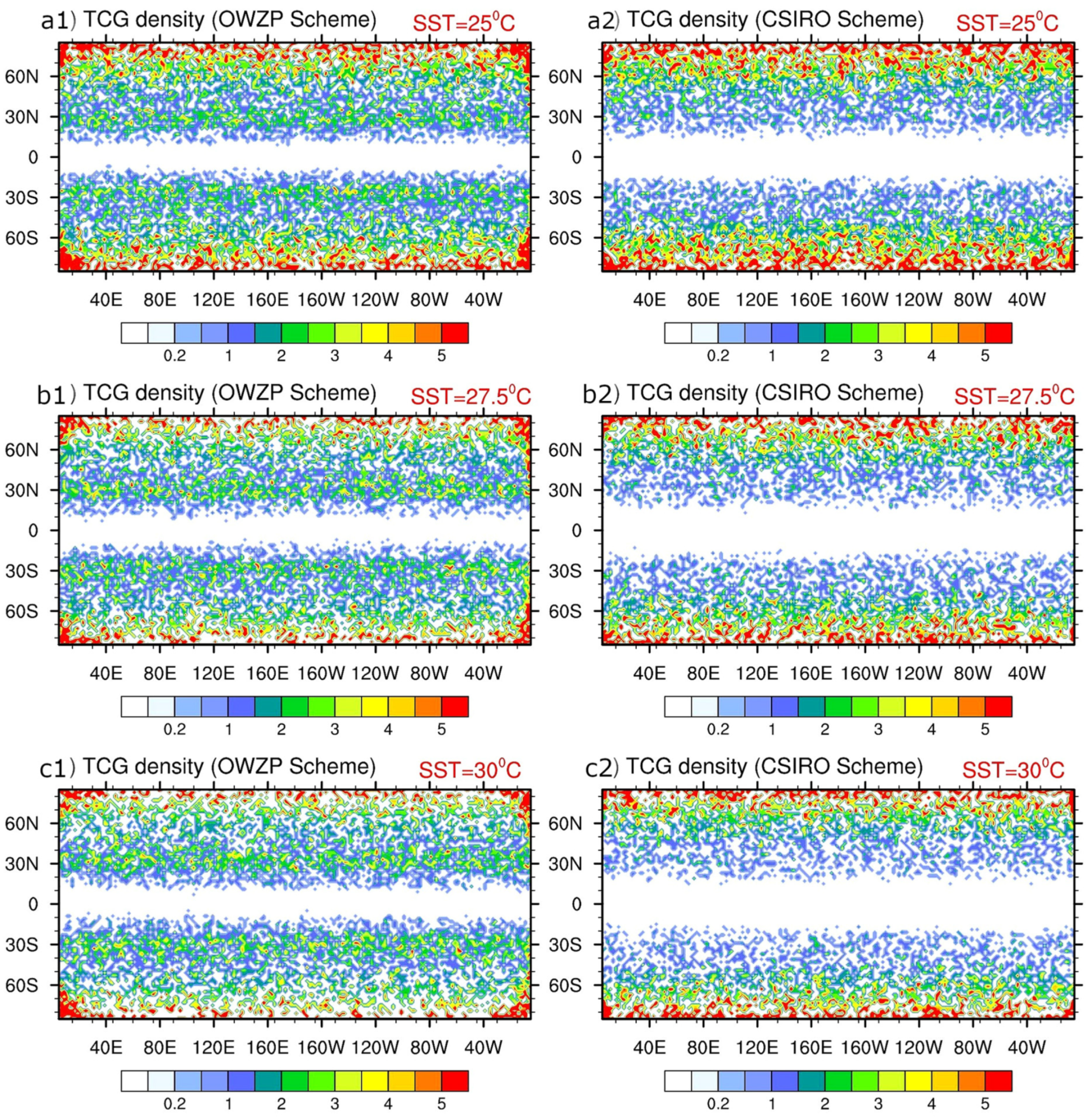
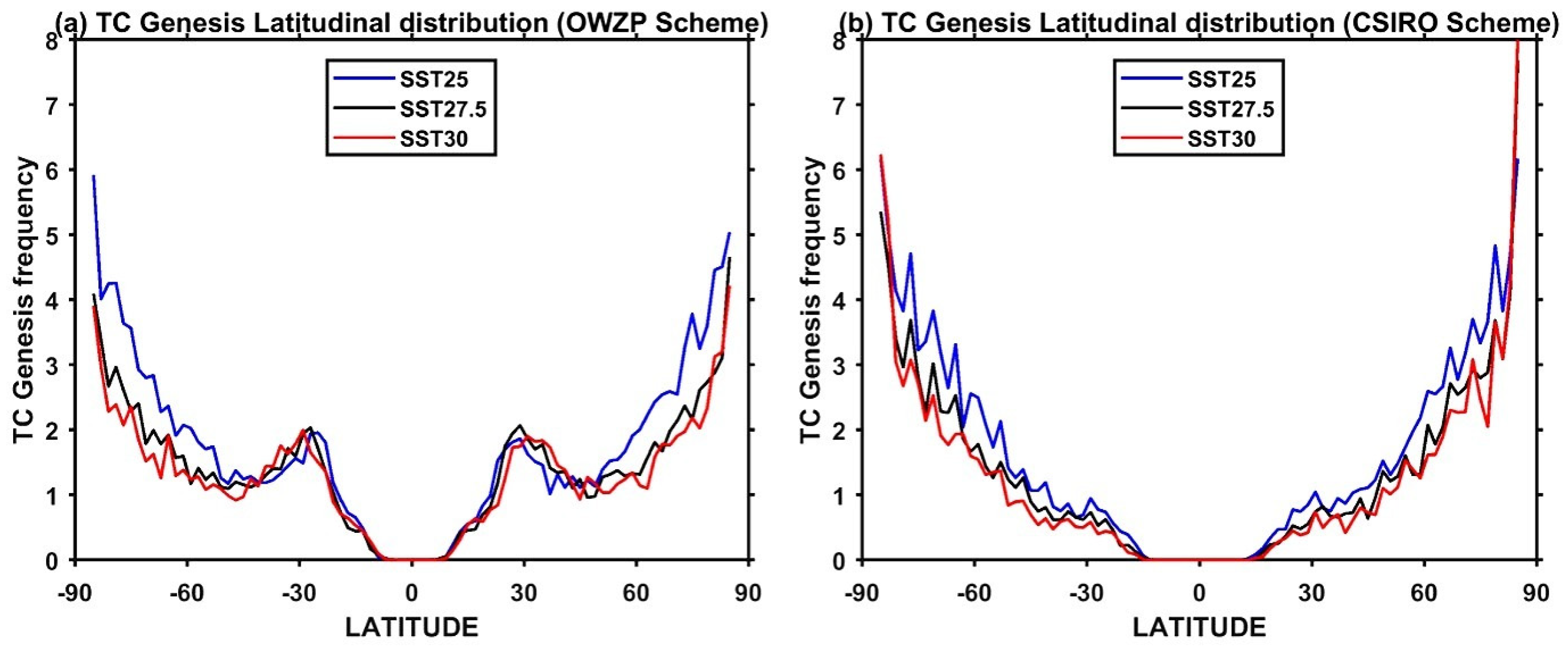
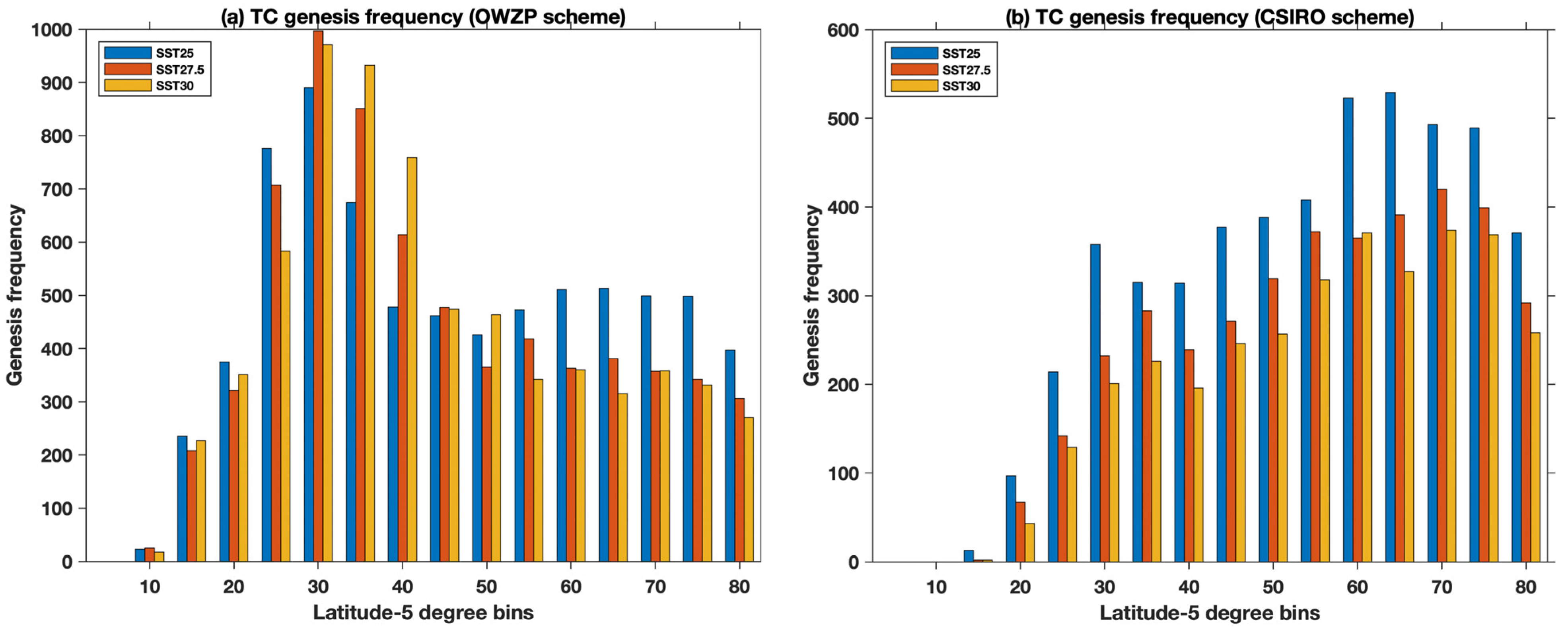
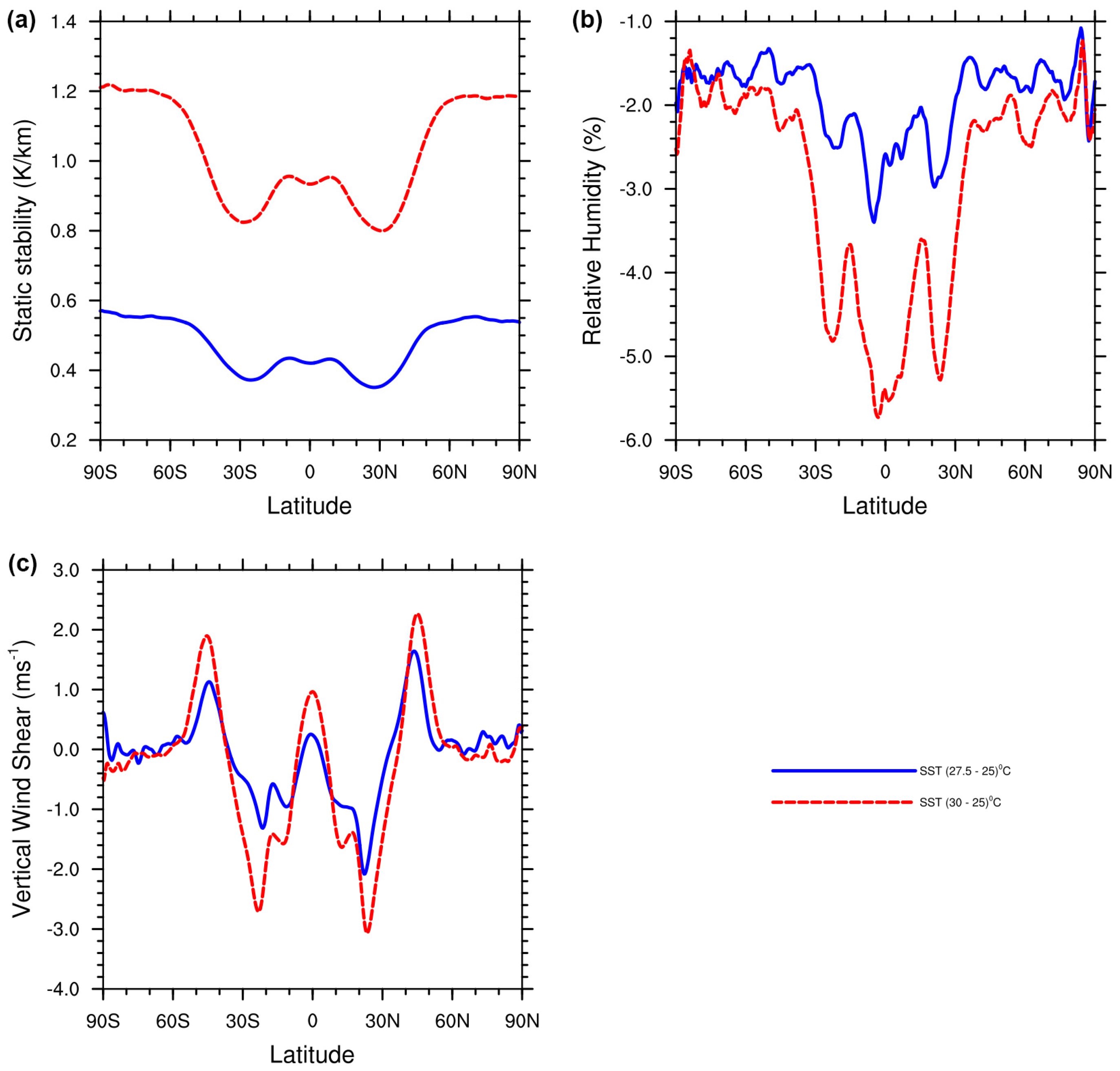
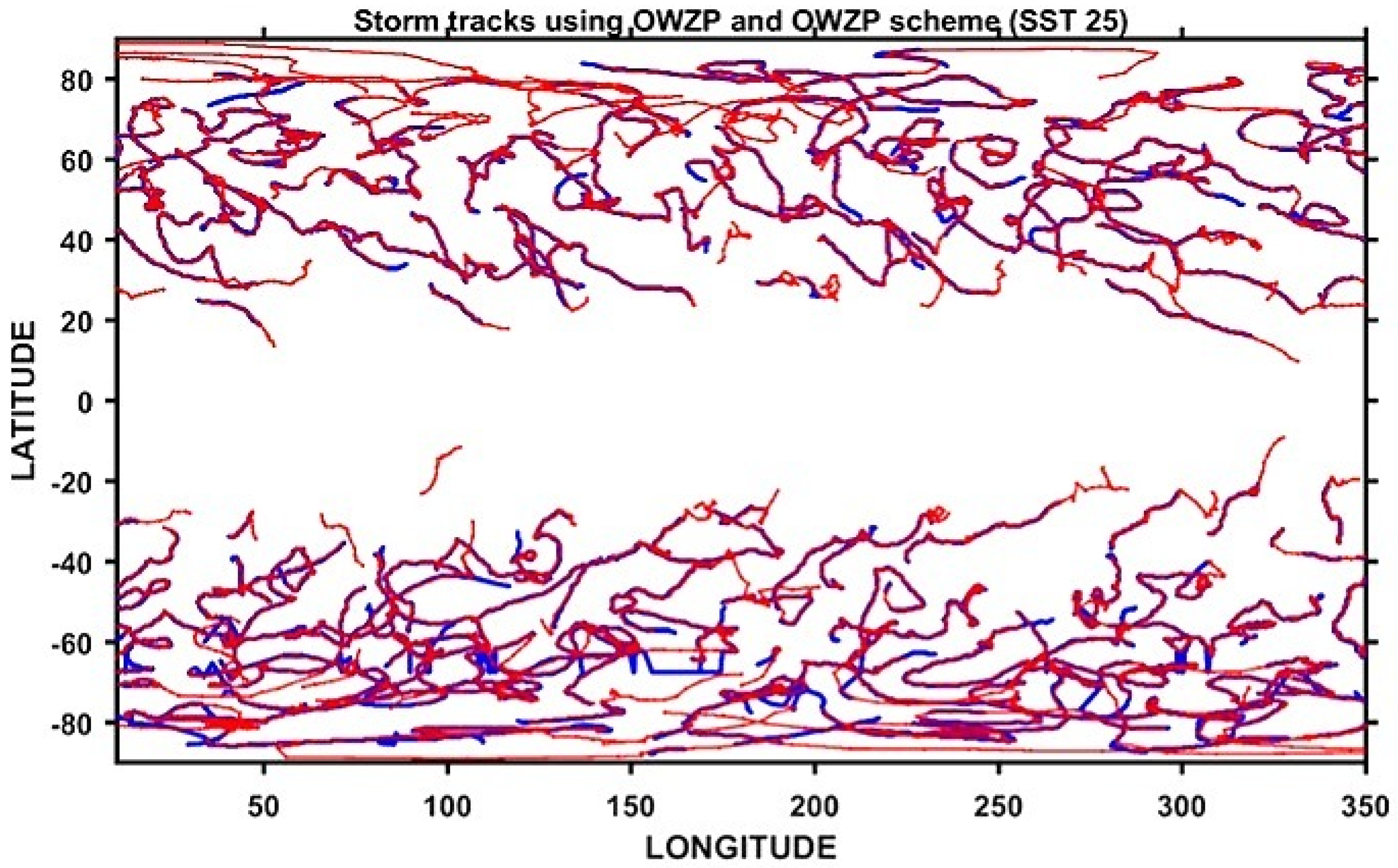
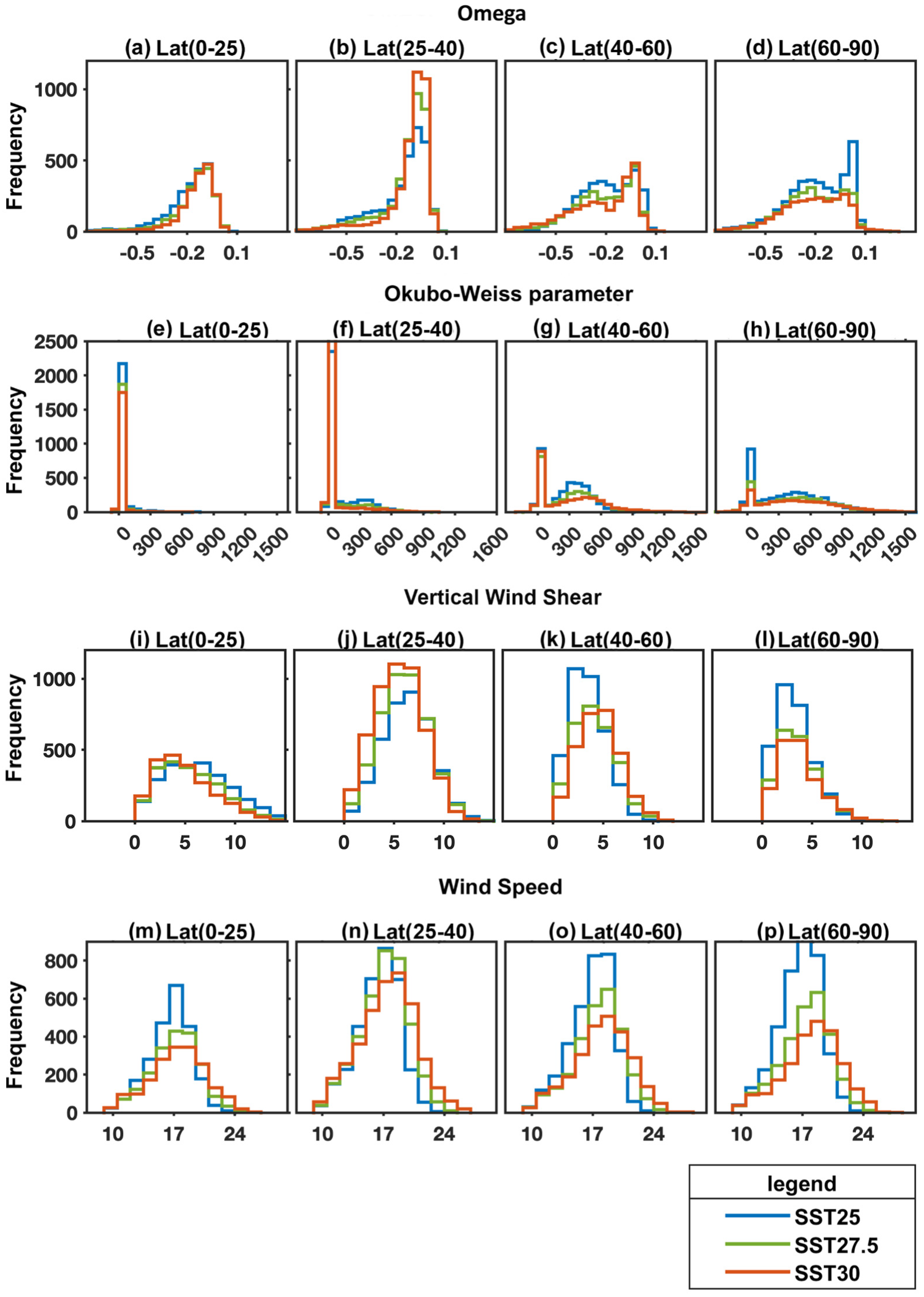
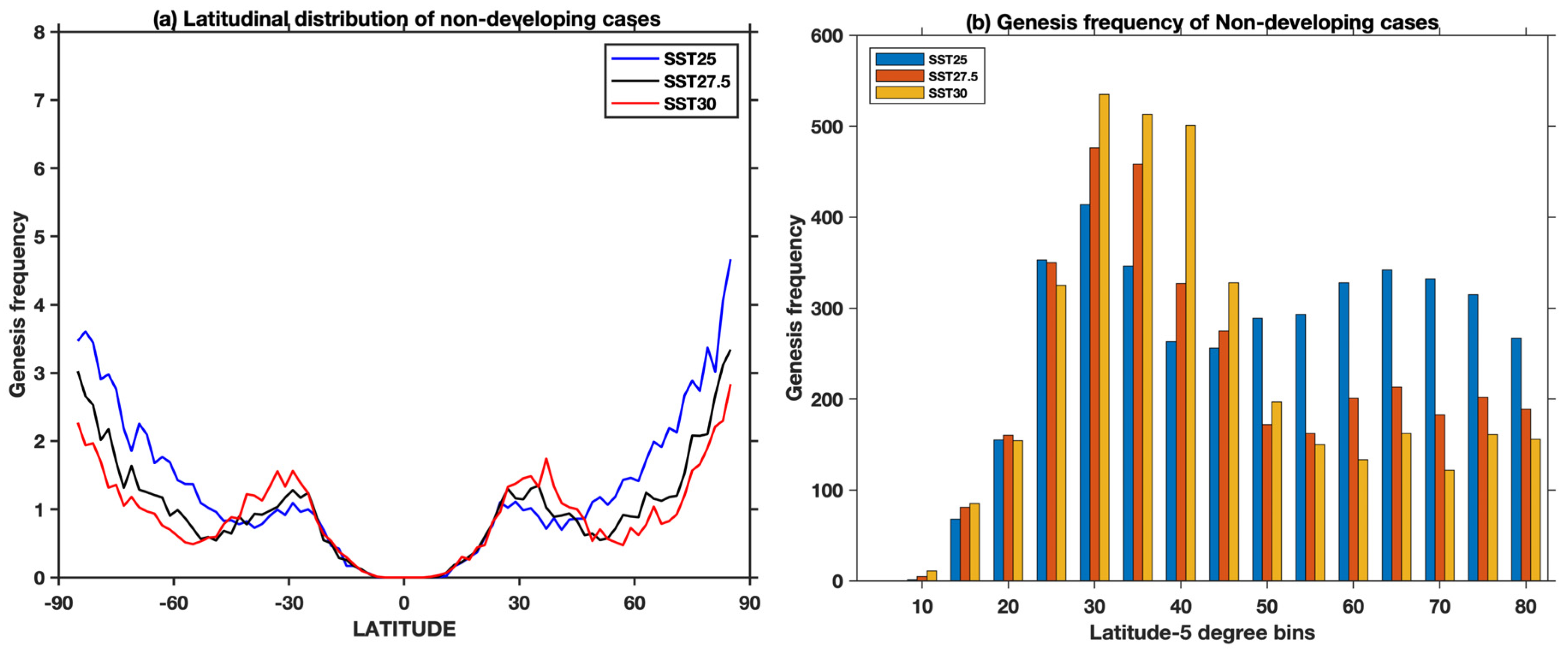
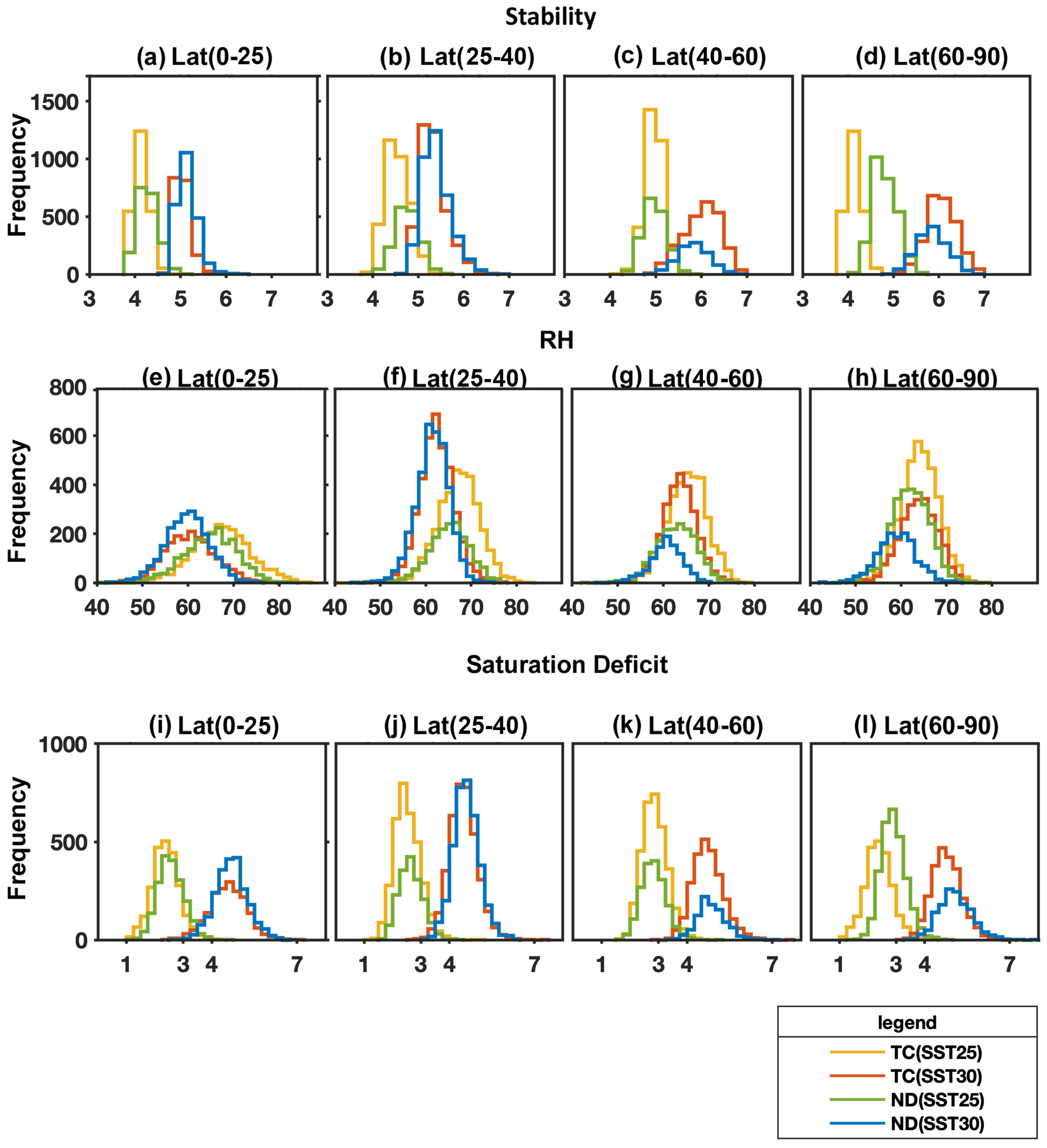
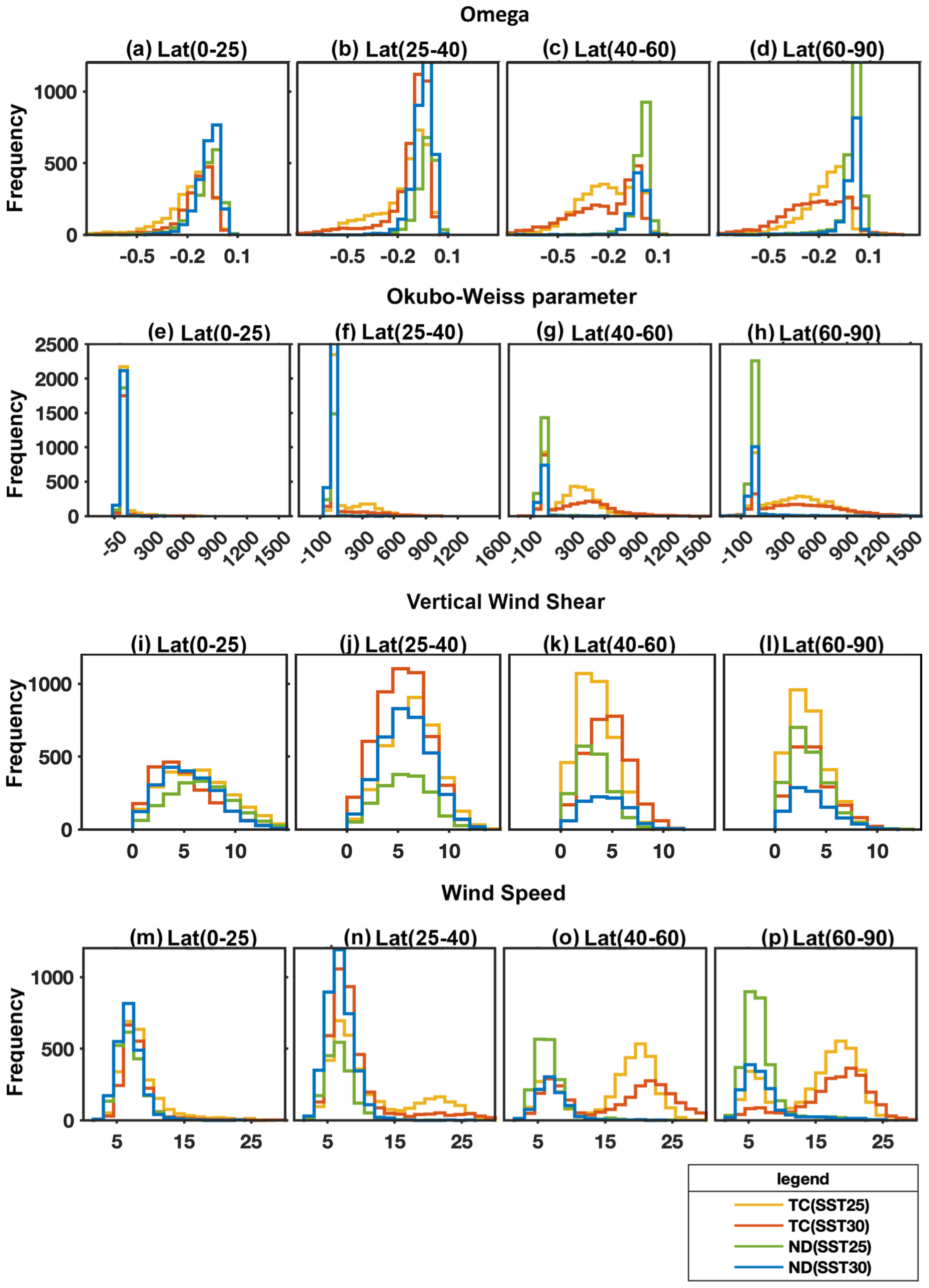
Table 1.
The global mean annual number of TCs and TDs for each of the aqua-planet simulations using the OWZP and CSIRO detection schemes.
Table 1.
The global mean annual number of TCs and TDs for each of the aqua-planet simulations using the OWZP and CSIRO detection schemes.
| Experiment | OWZP Scheme (TC) | CSIRO Scheme (TC) | OWZP (Greater than 10 m/s) | OWZP Scheme (TDs) | Non-Developing Cases (ND) |
|---|---|---|---|---|---|
| SST25 | 3218 | 2277 | 2583 | 5007 | 1789 |
| SST27.5 | 2929 | 1808 | 2286 | 4449 | 1520 |
| SST30 | 2923 | 1586 | 2197 | 4463 | 1540 |
Table 2.
Decision tree rules obtained after applying the C4.5 classification algorithm to the SST25 and SST30 experiments for different latitude bands.
Table 2.
Decision tree rules obtained after applying the C4.5 classification algorithm to the SST25 and SST30 experiments for different latitude bands.
| SST25 and SST30 (0–25) |
| 1. if RH > 65.43 then TC forms in SST25 2. if RH ≤ 65.43 and VWS ≤ 5.7 then TC forms in SST30 |
| SST25 and SST30 (25–40) |
| 1. if RH > 67 then TC forms in SST25 2. RH ≤ 67 and 10 < OW ≤ 70 then TC forms in SST30 3. if RH ≤ 67, OW > 70, and RH > 63 then TC forms in SST25 4. RH ≤ 67, OW > 70, RH < 63, and VWS < 6 then TC forms in SST30 |
| SST25 and SST30 (40–60) |
| 1. if OW > 568 then TC forms in SST30 2. if OW < 568, VWS < 4.3 then TC forms in SST25 3. if OW < 568, VWS >4.3, and RH > 66 then TC forms in SST25 4. if OW < 568, VWS >4.3, RH < 66, and OW > 353 then TC forms in SST30 |
| SST25 and SST30 (60–90) |
| 1. if WIND > 18 then TC forms in SST30 2. if WIND ≤ 18 then VWS ≤ 2.1 then TC forms in SST25 3. if WIND ≤ 18, VWS > 2.1, and VWS ≤ 6.5 then TC forms in SST25 4. if WIND ≤ 18, 6.5 < VWS ≤ 12 then TC forms in SST30 |
Publisher’s Note: MDPI stays neutral with regard to jurisdictional claims in published maps and institutional affiliations. |
© 2021 by the authors. Licensee MDPI, Basel, Switzerland. This article is an open access article distributed under the terms and conditions of the Creative Commons Attribution (CC BY) license (https://creativecommons.org/licenses/by/4.0/).
Share and Cite
MDPI and ACS Style
Raavi, P.H.; Walsh, K.J.E. Response of Tropical Cyclone Frequency to Sea Surface Temperatures Using Aqua-Planet Simulations. Oceans 2021, 2, 785-810. https://0-doi-org.brum.beds.ac.uk/10.3390/oceans2040045
AMA Style
Raavi PH, Walsh KJE. Response of Tropical Cyclone Frequency to Sea Surface Temperatures Using Aqua-Planet Simulations. Oceans. 2021; 2(4):785-810. https://0-doi-org.brum.beds.ac.uk/10.3390/oceans2040045
Chicago/Turabian StyleRaavi, Pavan Harika, and Kevin J. E. Walsh. 2021. "Response of Tropical Cyclone Frequency to Sea Surface Temperatures Using Aqua-Planet Simulations" Oceans 2, no. 4: 785-810. https://0-doi-org.brum.beds.ac.uk/10.3390/oceans2040045