Article

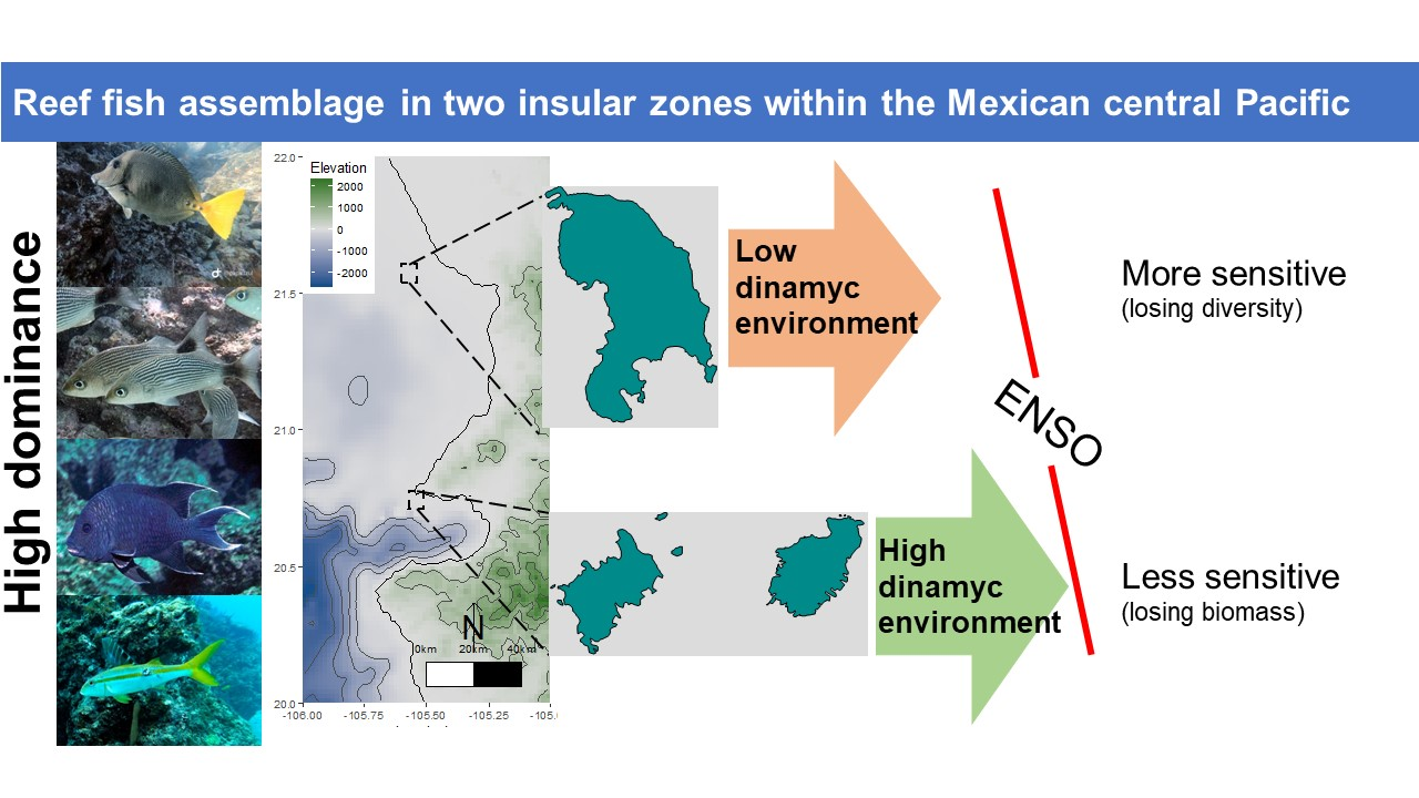
Reef Fish Assemblage in Two Insular Zones within the Mexican Central Pacific

by
Carlos Vladimir Pérez de-Silva
1,
Amílcar Leví Cupul-Magaña
1,*,
Alma Paola Rodríguez-Troncoso
1 and
Fabián Alejandro Rodríguez-Zaragoza
2
1
Laboratorio de Ecología Marina, Centro Universitario de la Costa, Universidad de Guadalajara, Av. Universidad de Guadalajara No. 203, Puerto Vallarta 48280, Jalisco, Mexico
2
Laboratorio de Ecología Molecular, Microbiología y Taxonomía (LEMITAX), Departamento de Ecología, Centro Universitario de Ciencias Biológicas y Agropecuarias, Universidad de Guadalajara, Camino Ramón Padilla Sánchez No. 2100 Nextipac, Zapopan 45110, Jalisco, Mexico
*
Author to whom correspondence should be addressed.
Submission received: 25 December 2021 / Revised: 4 May 2022 / Accepted: 17 May 2022 / Published: 23 May 2022

Abstract

:
Reefs fishes are sensitive to environmental changes, particularly in areas such as the Mexican Central Pacific (MCP), which has a high environmental variability favored by currents. This study assesses the temporal variation in ecological indicators of fishes in Marietas (MI) and Isabel islands (II) in the MCP during 2010–2017. Overall, 118 species were recorded at MI and 95 in II. The highest abundance was recorded in 2013 at MI, and in 2015 at II, with an observed sample coverage > 0.79 for all years. MI showed higher annual taxonomic distinctness and richness than II. Annual biomass and assemblages were different between years and islands. The changes in both islands’ community structure were influenced by ENSO events. A high proportion of the dissimilarity among years is represented in 10 species, and the difference among years for each island is given by rare species. Annually, community indicators (Δ+, q = 1, and q = 2) and physicochemical factors were not related except for q = 0 and the chlorophyll concentration; this is due to the inter-annual variation within the area. The variation in fish communities on both islands results from mesoscale phenomena that have a different effect on each island due to the characteristics of their shelf and oceanography.

Graphical Abstract

1. Introduction

Coral reefs are considered ecosystems with the highest primary productivity and biological diversity in the oceans [1]. In these areas, hermatypic coral species generate a complex topography that harbors associated species such as fish and invertebrates. This ecosystem and its associated organisms provide environmental services to human communities [2,3], contributing to their well-being and life quality [4]. Fish are considered a key taxonomic group in this ecosystem, as they fulfill diverse roles [5]. Changes in the richness and abundance of this group will affect relations within the ecosystem and its residents [6]. Among the factors that can modify reef fish populations are drastic changes in marine physicochemical factors [7,8,9,10,11] and the lack of regulation of fishing activities [12,13,14,15,16]; hence, the combination of these factors can trigger a decline in the number of species, abundance, and size of the individuals from resident fish populations. Tropical reef communities are threatened by poorly regulated human activities such as tourism and fishing, and natural mesoscale phenomena like El Niño Southern Oscillation events (ENSO) [3,17,18]. The reefs along the Mexican Central Pacific (MCP) are considered more sensitive to ENSO effects due to their isolation [19], making them more susceptible to changes in their ecological dynamics and diversity [20]. In transitional areas like the MCP and the entrance of the Gulf of California, natural populations have a tolerance to cyclical changes within an annual period [21,22], which is reflected in the reef communities including coral, invertebrates, and the seasonal abundance of reef fishes. However, the increase on both periodicity and intensity of mesoscale phenomena, combined with the pressure of extractive activities in this area, may compromise the functionality of the ecosystems and the well-being of coastal human populations. The implementation of global actions to prevent long-term changes in climate patterns is a priority for biodiversity conservation [23]; these actions do not aim to stop climate change, but to mitigate its effects on natural populations. The protection of specific areas and the promotion of a change in the legal status of natural protected areas, including their marine regions (e.g., Marine Protected Areas, MPAs) are tools that allow the establishment of zones and concrete actions that favor the conservation of ecosystems and the species that reside in them.
The benefits of an MPA can be quantified in both the short- and long-term after implementation [24]. Among the indicators for assessing the efficiency of MPAs are species richness, the abundance of individuals [25,26], and taxonomic complexity [6,27]. Nevertheless, comparing efficiency among MPAs can be complex because each one has different management objectives and strategies as well as monitoring techniques relevant for assessing the effectiveness of protection afforded by the MPA. These limitations have resulted in new comparative techniques to evaluate changes in the community [28,29], based on the magnitudes and proportion of richness and abundance expressed in the number of species. The variability of these indicators in the fish community over time reflects changes in the reef community; in addition, a comparison between natural areas creates a baseline for future management actions. Therefore, the objective of this study is to evaluate changes in the reef fish diversity in two MCP insular fish communities during eight years (from 2010 to 2017) as well as the changes that occur in the reef fish community structure and to relate these with local environmental conditions in each island.

2. Materials and Methods
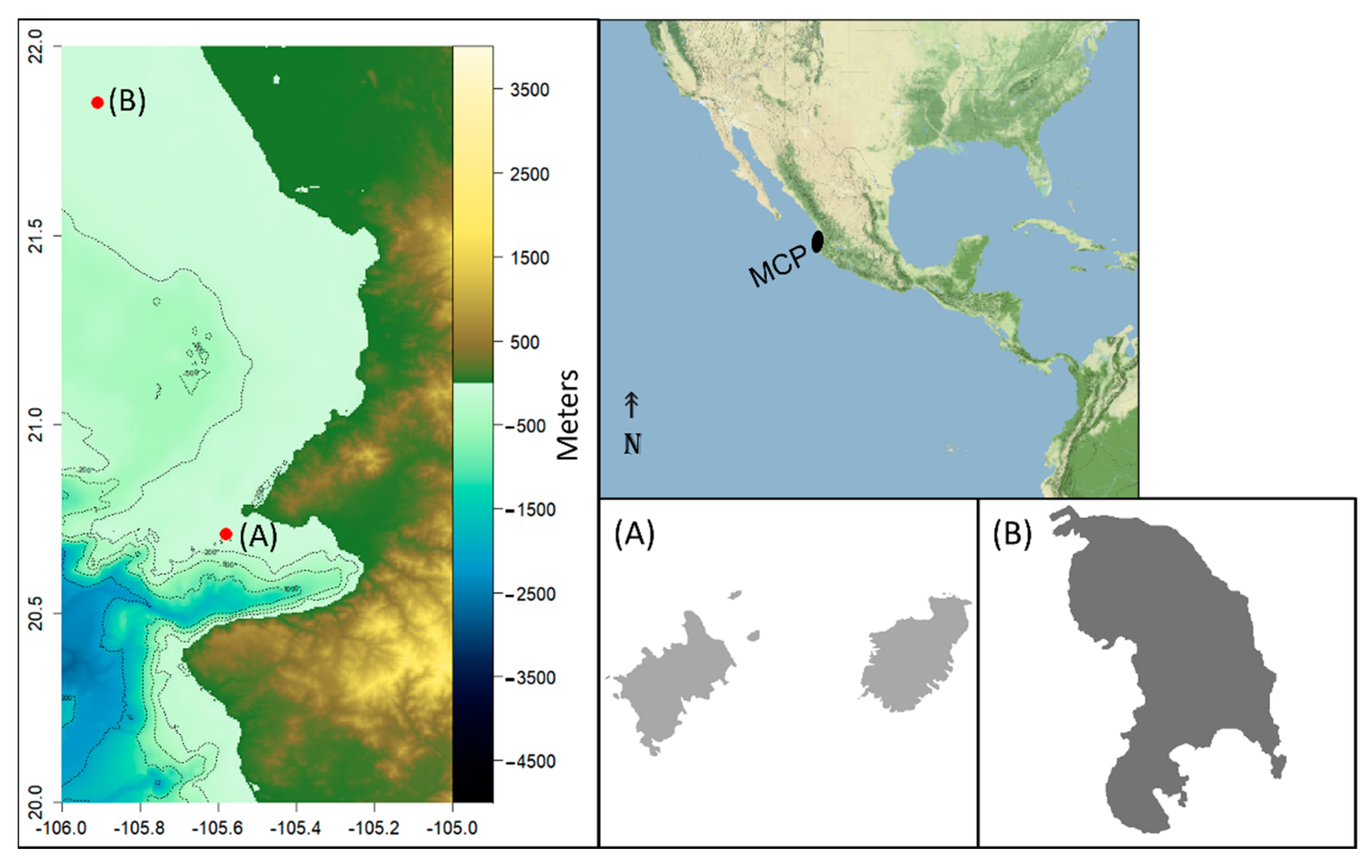
2.1. Study Area

The MCP has several island complexes, among which the Isabel Island and Marietas Islands stand out due to their location within an oceanographic transition zone, and their use in non-extractive activities. Both islands are included in the list of the Comisión Nacional de Areas Naturales Protegidas (CONANP) under the category of national park, although they have different conservation objectives and contrasting geographic and geologic characteristics.
Isla Isabel National Park (II; 25°52′ N, 105°54′ W) is located 28 km off the coast of the state of Nayarit, within the MCP (Figure 1). This area only protects terrestrial territory, as it is mainly focused on the protection of sea bird species [30]. The island is surrounded by a shallow continental platform and extends to the Marietas islands archipelago, and harbors important coral reef patches. Temporary fishing camps are the only human population on this island.
Marietas islands (MI; 20°42′47″ N, 105°33′18″ W) is an archipelago consisting of two main islands (Isla Larga and Isla Redonda) with a series of small islets located 6 km from the coast of Nayarit and 130 km south of Isabel Island. This area has a special protection status as a national park [31] (Figure 1), which includes the marine zone that surrounds them. The continental shelf on these islands is short and near to the Bahia de Banderas deep zone [32].
Both sites are influenced by the Costa Rica Coastal Current, the California Current, and the Gulf of California water mass [33]. One of the main differences between these islands is the absence of protection in the marine portion of II. The differences in management activities between the islands provide an appropriate scenario for a comparison between these zones.

2.2. Fieldwork

From 2010 to 2017, underwater surveys were performed using scuba diving in MI and II; these were focused mainly on fish species found in the water column and the most conspicuous cryptic species. Reef fish species’ abundance and size were recorded using 25 m × 4 m (100 m2) belt-transects. During the surveys performed in 2010 and 2011 in both islands, the observation area was only 40 m2 (20 m × 2 m). The sampling effort was different for each island; therefore, community indicators were analyzed independently for each insular system.

2.3. Species-Abundance Analysis

The representativeness of the reef fish assemblage and its diversity were evaluated through sample completeness (SC) and asymptotic profile using the number of individuals as an observation, calculating the Hill numbers with 1000 permutations [34]. Based on this methodology, for each island and each year, the sample coverage (SC), number of species (q = 0: S, number of species), the effective number of common species (q = 1: exponential of Shannon entropy), the effective number of dominant species (q = 2: Gini–Simpson index), and the rare species indicator, given by the difference between q = 0 and q = 1, were measured. The results were contrasted using the Four-Step methodology [29]. The extrapolations of these indicators were calculated to double the abundance of each year (number of individuals) for each island [34] and a cut-off SC value was considered for comparisons between islands by a permutational univariate analysis of variance to establish differences among q = 0, 1, and 2 indicators between islands. The interpolation and extrapolation analyses were performed on the R-project platform with the “iNext” package [35].

2.4. Taxonomic Distinctness

Taxonomic distinctness (Δ+) and its variation (Λ+) [27] were calculated with the annual species composition for each island (presence–absence) and their taxonomic classification according to FishBase. The taxonomic distinctness between islands was compared using a global model built with the taxonomic list of both insular systems. The taxonomic distinctness models were visualized with a funnel and ellipsoid graphs showing the Δ+, Λ+, and species richness (S) relationships. These models were performed using 1000 permutations. Statistics were performed in the Primer-6 [36] and the R-project software using the Vegan package for ecological analysis [37] and the rFishbase [38] package for the taxonomic classification.

2.5. Biomass Data Analysis

Fish species biomass was calculated using the Von-Bertalanffy allometric weight equation (W = aLb, where W: individual weight; L: observed length; a: scaling constant; b: allometric growth parameter), using a and b parameters obtained from FishBase [39]. Overall biomass per individual and per species was taken as a measure of abundance to perform the multivariate analyses that describe the inter-annual changes in the fish assemblage composition in each site.
The annual variation in biomass per square meter was evaluated independently on each of the islands using a univariate permutational analysis of variance generated from an Euclidean distance matrix. Differences between years were highlighted using pairwise comparisons. To establish significant differences in the reef fish assemblage structure over the years in each island (Y = µ + Yi + Ɛi), a one-way permutational multivariate analysis of variance (PERMANOVA) was performed using the Bray–Curtis resemblance matrix and each transect as a sample for each year. Pairwise comparisons between group levels with corrections for multiple testing [40] were performed to identify the years that were different. Both analyses were performed using 1000 permutations. With a Bray–Curtis similarity matrix obtained from each specie’s annual average biomass, a principal coordinate analysis (PCoA) was carried out to visualize the interannual changes of the assemblage of reef fishes as an ecological successional model. The species with the highest contribution to dissimilarity among the annual assemblages were obtained from a percentage similarity analysis (SIMPER). Based on the paired comparisons, the contribution per species was averaged, and those species that overall accounted for more than 50% of the dissimilarity in each year for each island were displayed in a box-plot graph. All the analyses were performed using the R-project and the packages “Vegan” [37] and “RVAideMemoire” [40].

2.6. Influence of Environmental Variables

The influence of environmental variables was evaluated with a multiple linear model in which the ecological indicators of a total number of species (q = 0), high abundance species (q = 1), dominant species (q = 2), and the value of taxonomic distinctiveness (Δ+) were used as the dependent variables. The predictive variables were the annual average sea surface temperature (SST), chlorophyll (Chl), and primary productivity (Pp) obtained from the online NOAA ERDDAP database [41]. To avoid multicollinearity, a covariance test between the dependent and predictive variables was used to reduce covariance, and ecological indicators and environmental variables with correlation values greater than 90% were discarded.

3. Results

3.1. Species-Abundance Data Analysis

The total abundance recorded for MI was 295,290 individuals, corresponding to 118 species, 87 genera, 46 families, and 14 orders. For II, the total number of reef fish individuals was 51,341, belonging to 95 species, 90 genera, 38 families, and 10 orders. The Four-Step evaluation showed the following:
(1)
The pattern of the sample coverage with respect to the q = 0, 1, and two indicators show an increasing tendency (Figure S1a) for the order of total species indicator (q < 0.5); i.e., the sample coverage was lower for MI, meaning that in this island there are more unrecorded species. At MI, the lowest SC value was recorded for the year 2010 (79%, Table 1, Figure S1a), which implies that the remaining 21% accounts for a total of 17 species that were not detected according to the asymptotic model; in contrast, 2015 presented the highest SC (95%), representing an absence of three species accounting for 5% of the SC. Meanwhile, II showed the highest annual SC value corresponding to 2014 (97%), reflecting a difference from the asymptotic model of fewer than one species. However, 2011 and 2017 presented the lowest SC values (86%) for this island, representing a total of 10 and seven species not observed, respectively, according to the asymptotic model (Table 1).
(2)
The comparison of each order of q = 1 and 2 showed that the numbers of both abundant and dominant species were the same as those from the asymptotic model in both islands (Table 1, Figure S1a,b). At MI, the year 2011 had the highest value of abundant species (17.4) and the year 2010 showed the highest value of dominant species (10.2). In contrast, the lowest values of both indicators of abundant and dominant species were recorded in 2015 with 13.2 and 6.9 species, respectively; these values suggest that for this year there was a total of 68 rare species (q = 0 − q = 1). At II, the same indicators showed that the year 2011 had the highest number of abundant (19.6) and dominant (14) species, while 2012 resulted in the lowest value of these indicators with 9.8 abundant and 4.4 dominant species, and a total of 50.2 rare species.
(3)
The non-asymptotic coverage-based rarefaction and extrapolation analysis (Table 1, Figure S1a,b) shows that although our data are insufficient to infer the true richness of the whole set, inference and significance testing can be extended to an SC cut-off value for both islands of SCmax ≥ 99%. At this confidence level, at MI the year 2011 reached the highest richness (86.27 species), followed by 2016 (77.05), and the lowest was found in 2015 (69). In contrast, at II the highest richness value was obtained in the year 2013 (69.54), followed by 2011 (66.95) and the lowest values were observed in 2014 (40.06).
(4)
Under the coverage value of 99%, the evenness profile and Pielou’s measure (Table 1, Figure S1a,b) were similar in the three q = 1, 2, 3 levels (p-value = 0.05); nevertheless, at II, the confidence intervals of the evenness profile show a wider range among the years, which implies more year-on-year variation at this island (Figure S1b).

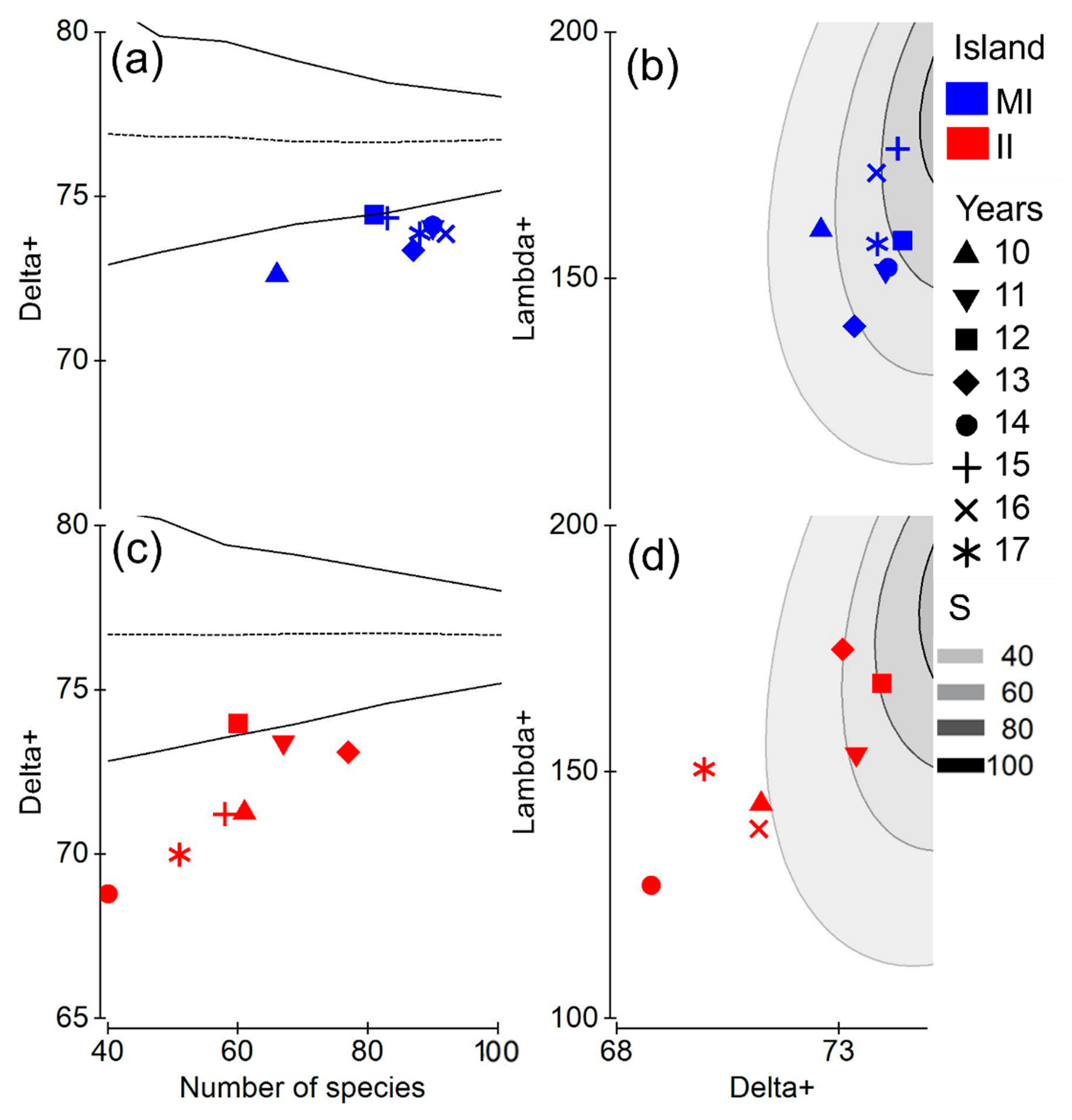
3.2. Taxonomic Distinctness

The combined taxonomic model of both sites resulted in an average Δ+ = 76. Only in 2012 did both islands show values within those expected by the global model. Only the year 2012 obtained expected proportions of Δ+ and S shown in the funnel plot for both islands (Figure 2a,c). At MI, all the years evaluated were within the values expected by the ellipsoid model, whereas at II, years 2010, 2014, 2016, and 2017 were outside the expected values (Figure 2b,d). From species recorded at MI, the values of the indicators are within those expected by the model (ellipsoid). On the other hand, at II, the values of S and Δ+ are lower than expected (both in the funnel and in the ellipsoid). The above shows that II has a lower taxonomic diversity.
At II, the average Δ+ was 71.66, with the years 2013 and 2011 showing the highest values of observed species with 77 and 67, respectively, and 2012 with the highest value of Δ+ (Figure 2c). In addition, only these years were within the expected number of species suggested by the global model (Figure 2d). The years 2014, 2017, 2015, and 2010 presented the lowest values of these indicators (Figure 2c). Among the years with the lowest Δ+ values, 2010 stands out because it has a similar richness to 2012; however, in this year, the relation between species is in the lower taxonomic levels.

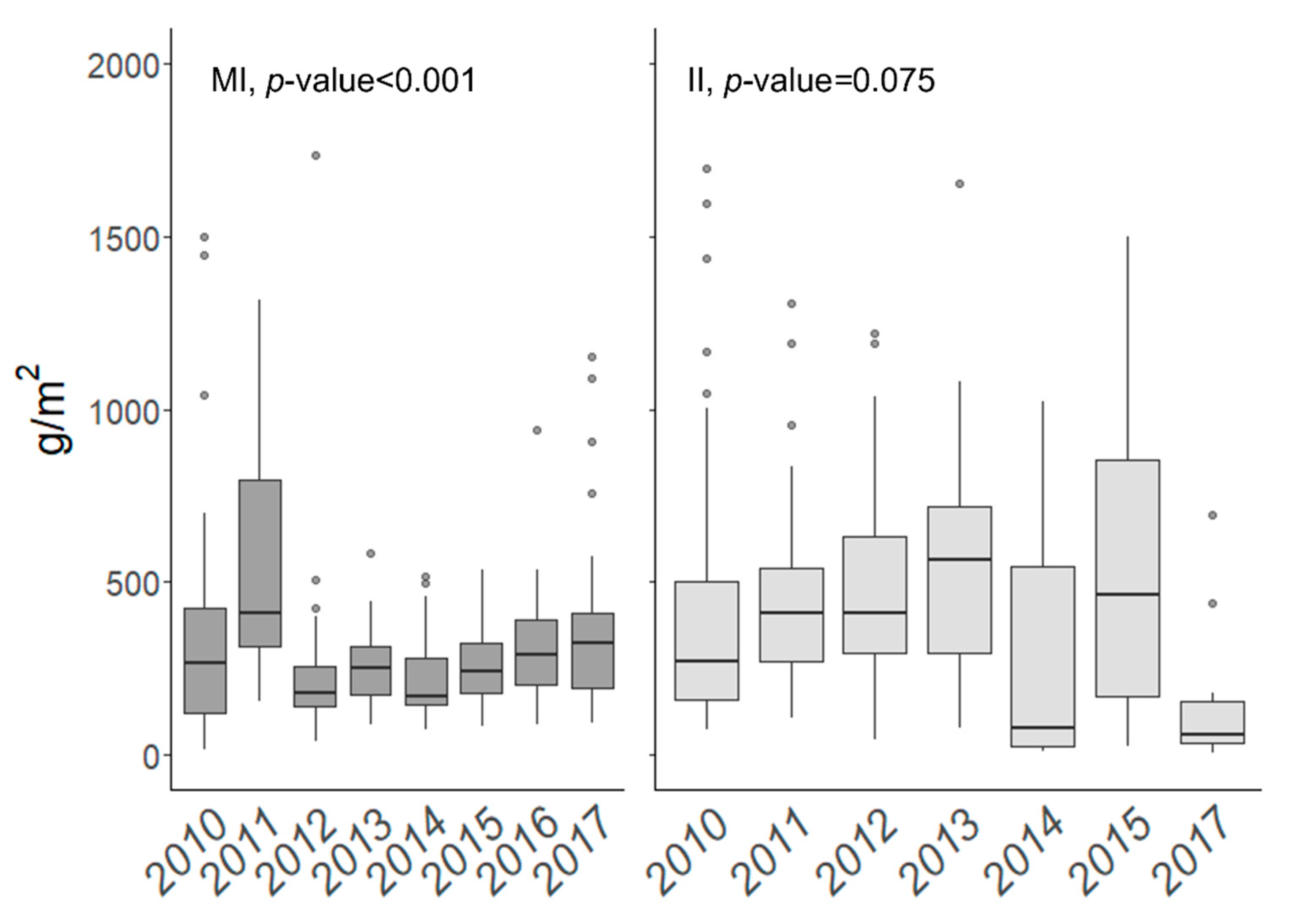
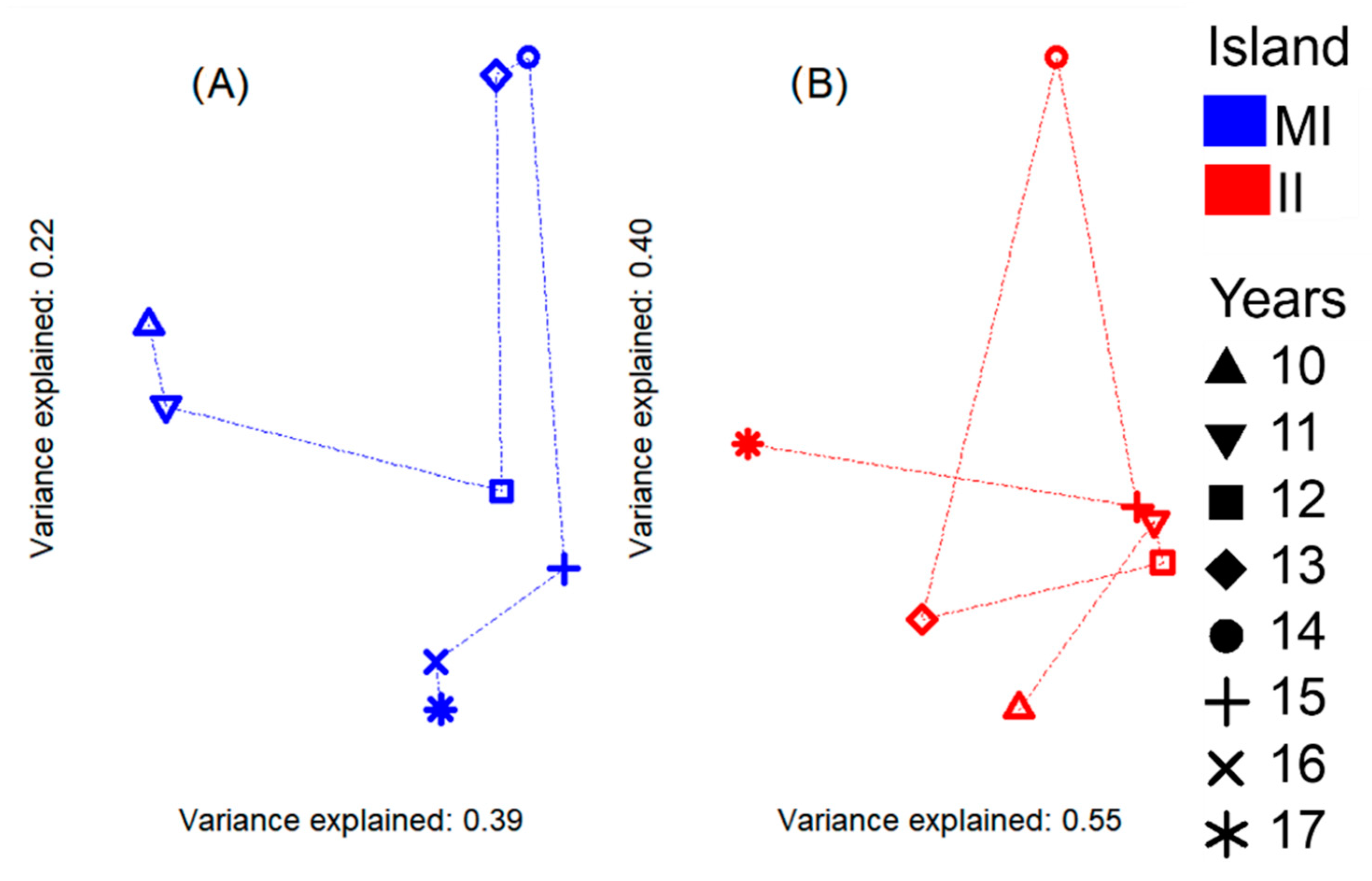
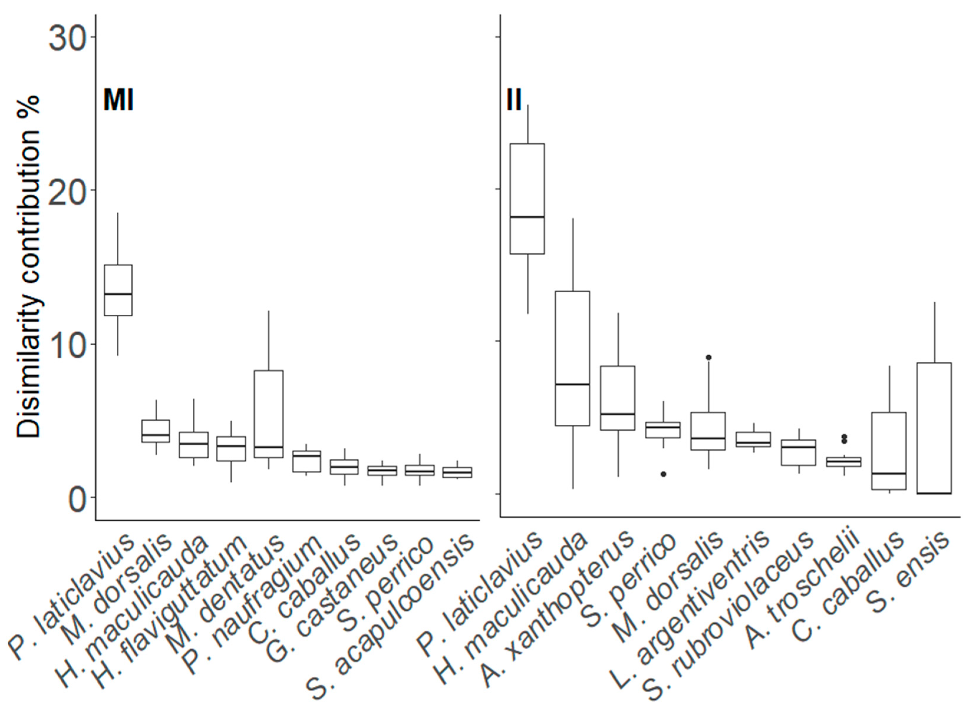
3.3. Year-to-Year Biomass Variation

3.3.1. Marietas Islands

The MI average biomass was lower among both islands (345 ± 329 g m−2). The biomass comparisons at MI showed annual differences (pseudo-F = 5.22, p-value < 0.001, Figure 3); these were significantly different between 2011 and all other years except 2017 and between 2014 and 2017 and 2010 and 2014 (p-values < 0.05, Table S1a). The comparison of the assemblage of the reef fish showed that there were significant differences in the annual composition (pseudo-F = 4.53, p-value < 0.001), while the a posteriori tests showed that 2017 was different in comparison with the years 2011, 2013, 2015, and 2016 (Table S1b).
The ecological succession model built for this island, which explains 61% of the variation, shows that the year 2017 was farther away from the center of the ordination than the rest of the years (Figure 4a), representing that the species composition in this year was more different than the other years. The consecutive years that were farthest apart were 2014–2015, where the distance between these entities was the largest. Finally, 2016 and 2017 are relatively close to each other in the ordination (Figure 4a). The SIMPER analysis for MI showed that the average between-group dissimilarity in the paired comparison was 68 ± 0.72%. The main species that contributed to dissimilarity were: Prionurus laticlavius, Microspathodon dorsalis, Haemulon maculicauda, Haemulon flaviguttatum, Mulloidichthys dentatus, Pseudobalistes naufragium, Caranx caballus, Gymnothorax castaneus, Scarus perrico, and Stegastes acapulcoensis. These species represent a total average dissimilarity of 39 ± 27% (Figure 5). The most important changes in assemblages occurred between 2010 and 2015, with a dissimilarity value of 80% (Table S2a).

3.3.2. Isabel Island

Isabel Island showed higher average fish biomass for all years (567.4 ± 729.6 g m−2). The annual biomass comparison showed no significant differences (pseudo-F = 1.96, p-value = 0.075). Despite this, one-way PERMANOVA analysis using transects as annual samples found significant differences between years (pseudo-F = 4.11, p-value = 0.001), and an a posteriori test shows that the differences were between 2011 and 2012; 2013 with 2010, 2011, and 2012; 2015 with 2010 and 2011, and 2017 with 2011, 2012, and 2015 (Table S1b). The ecological succession model, which builds from the annual biomass average per species, explains 95% of the variation within assemblages, where the years 2011, 2012, and 2015 are closer to each other. In contrast, 2014, which showed no similarity with any of the years, as well as 2010, which showed similarity with only two years, and 2017, which showed similarity with only three years, were found to be far from the rest of the years (Table S1b, Figure 4b). There is a disparity between the comparison tests and the ecological succession model, because the permutational tests used the transects as samples, whereas the PCoA only reflected the annual changes. On this island, more years were different from each other. Neither the a posteriori tests nor the pattern between the years suggested by the model show an evident succession between the community changes at II. This suggests that the assemblage on this island is not homogeneous and that there are important annual changes. This is also corroborated in the SIMPER analysis, where the average dissimilarity was 84 ± 5% between paired comparisons. The species that contributed most to the dissimilarity between years were: P. laticlavius, H. maculicauda, Acanthurus xantopterus, S. perrico, M. dorsalis, Lutjanus argentiventris, Scarus rubroviolaceus, Abudefduf troschelli, C. caballus, and Sphyraena ensis. These species represent a combined dissimilarity percentage of 48 ± 27% between the years (Figure 5). The paired comparisons of 2011–2014 and 2012–2014, showed a dissimilarity value of 91%, suggesting that it is during these transition periods that the greatest changes in the assemblage occur (Table S2b).

3.4. Influence of Environmental Variables on the Community Indicators

The evaluation of the influence of environmental variables on the ecological indicators showed that on an annual basis, only chlorophyll displayed a significant relationship with the observed richness (q = 0, p-value = 0.049), while the rest of the comparisons with the ecological indicators and the same oceanographic variables were not significant (Tables S3 and S4).

4. Discussion

The evaluation of the diversity of the reef fish assemblage of both islands carried out over the years represents > 79% of the total diversity in certain years, particularly in 2010 for MI, where the lowest SC was observed (Table 1). The Hill number permutation methodology suggested by Chao, the conclusions and statistical assumptions are based on the lowest value of the diversity captured, in this case the sample coverage was 79% of what was expected for the poorest year of 2010, possibly due to the sample effort; however, the rest of the indicators recorded and calculated were within the general trend for this island.
The asymptotical model for the year 2010 showed the difference between the observed and the expected values (q = 0, Table 1), but not for the abundant and rare species (q = 1, 2); hence, it is assumed that even though the diversity was poorly represented in one year, the assumptions made for this year are over the 79% of the total species diversity [29]. Despite 2010, we can observe that in MI, most years have higher diversity than II in the three “q” orders, and when the islands are compared to the same SC cut-off level the same tendency occurs, showing that for 99% of the diversity (interpolated/extrapolated) MI has a higher diversity of species than II.
Differences between the variation of the number of species was likely caused by MI having a wider range of environmental variation (i.e., SST: 25.94–28.67 °C; PP: 1011–11982 mgC m−2 day−1; Table S4) [42,43,44], due to the proximity to the submarine canyon of Bahia de Banderas. This promotes a greater flow of water that, together with upwellings, generates higher dynamics between the surface and deep nutrient-rich waters with lower temperatures [45], increasing the diversity measured in the number of species at the three levels of q.
However, all indicators did not show differences among islands. Pielou’s evenness reflected the dominance of one or several species in the assemblage; in the case of MI and II, the low values of evenness are because for all species, dominance is held by no more than 12 species (<15% of the total richness) [36]. Similar values have been observed in other works where geographic characteristics are used as a source of variation for reef fish assemblages [46,47]; those find evenness values similar to this work despite variation among the other ecological indicators. The lack of variation in evenness indicators can be interpreted as a replacement in the proportion of rare species and compensation for species substitution between years. These changes may have maintained the stability of the assemblage in the face of certain perturbations so that such substitutions (if they exist) may have taken place between taxonomic groups that are close to each other and, obviously, these substitutions will affect the rest of the ecological indicators differently on each island.
The annual assemblage analyses of the Δ+ differ from the global models in both island systems despite their protection status, particularly at II, which implies that there is a level of degradation on both islands [48]. MI is in a dynamic coastal zone [49]; thus, the annual stability of the fish community reflects that resident species are acclimated to inter-annual environmental variation. Therefore, in the presence of mesoscale events (e.g., ENSO), it is more likely that their population numbers and, hence, the proportion of fish on these reefs will not be severely affected.
On the contrary, II, a place with lower Δ+ values, is prone to a loss of taxonomic distinctiveness, which has been observed in other Mexican reefs and is attributed to increasing predators caused by disturbances [6]. In 2011, the MCP was affected by an intense ENSO cold phase, which increased the availability of food for fish larvae. The effects can be observed the next year (2012) in the higher richness and biomass of fish (Table 1) and prey availability for organisms with higher trophic levels. However, in subsequent years, the lack of food supply and increase in the number of predators generated a reduction in biomass and taxonomic distinctness, which is evident in 2014 when the lowest values of taxonomic distinctness for both sites were observed. By generating a taxonomic model that considers the species presence or absence in both sites (Figure 2a,c), it is possible to make an adequate comparison between the two study areas. However, it is important to include abundance.
The successive annual trajectories shown in the PCoA (Figure 4a,b) highlight a change in the species composition of both reef fish assemblages. At both islands, differences observed in 2011, 2012, and 2015 can be attributed to ENSO events. II exhibits an erratic pattern in the assemblage, whereas MI’s changing pattern is consecutive. The trajectories generated in this study show that the most evident changes that occurred in the assemblages coincide in both islands, one during 2011–2012 and another during 2014–2015 (Figure 4), and are related to mesoscale events (2011–2012 La Niña and 2014–2015 a strong El Niño; Figure S2), which are particular to tropical and sub-tropical zones [50]. Notably, other studies have also demonstrated that environmental variation resulting from mesoscale phenomena impacts the years after such phenomena have occurred in a particular area [51].
In both islands over the years, abundance (q = 0, 1, and 2) and biomass (SIMPER) representations showed that ~12 species (<15% of the total recorded species) dominated the reef fish assemblage. These dominant species coincide with the characteristic fishes of the MCP [39,52], while the rest are considered rare species due to their proportion of representativeness (SIMPER values < 3%). Given the high number of rare species observed, changes in the fish assemblage on both islands depend on the ratio of the abundance and biomass of rare species, which are more than 60 in all years (Table S1a,b). Therefore, areas with a low number of dominant species (q = 2) are more vulnerable to environmental changes [53]. Between islands, chlorophyll and temperature influenced most of the ecological indicators (Table S3). These variables are not correlated to each other and differ in the islands due to the seabed and microscale events such as upwellings and algae blooms. First, MI is located in the edge of the continental platform at the entrance of Bahia de Banderas, which is characterized by a deep canyon (>1000 m) that brings cold and nutrient-rich waters to the surface, and is also influenced by internal waves [42] that generate a dynamic environment with upwellings in the area [54].
Despite the lack of correlation between the annual environmental measurements and the ecological indicators, events like El Niño influence both the richness (q = 0) and taxonomic distinctiveness (Δ+) of reef fishes on a yearly basis in both islands. The annual number of species per island is related to Chl, an environmental variable related to the availability of food for fish populations [55,56]. On an annual basis, the oceanographic variation in the MCP is cyclical, with a warm nutrient-poor phase with a deep thermocline and a cold nutrient-rich phase with intense upwelling processes along the coast [43,57], the combination of both seasons in one single annual value causes that between year-to-year comparisons have less variance and, therefore, statistically presents no differences for those oceanographic measurements.
Geographically in the northern area of the MCP, Isabel Island was characterized by a lower Chl concentration and higher SST (Table S4). These environmental characteristics are the result of the morphologies of the seabed in each of the islands; II is centered on a wide continental shelf, which decreases the dynamics and exchange with deeper waters (>100 km wide, Figure 1); these shallow waters suppress upwelling events, resulting in a deeper thermocline, nutricline [57], and longer-duration thermal anomalies. Particularly, the increase in the ENSO warm phase (2015, Figure S2) had a noticeable effect on the decrease of Chl and was also related to the total richness (q = 0) and the increase in species dominance for the island (q = 2). Over the years, tropical areas have shown relative thermal stability, benefiting fishes in these areas. However, changes in the frequency and intensity of mesoscale events compromise the environmental stability of these ecosystems [58,59]. The decrease in temperature in 2011 and the increased temperature in 2015 influenced other environmental conditions (Chl, PP, Table S4) and, consequently, the fish assemblages that are not acclimatized to such short-term variations. Indeed, II exhibited a lower number of species (q = 0), a higher proportion of dominant species (q = 2), and low taxonomic distinctness (Δ+). Therefore, mesoscale events affect II more than MI, contributing to the degradation of the fish assemblage that is already sensitive to environmental changes.
Both islands are located within a transition zone where three ecoregions [60], and two major ocean currents influence the area [21,22,44]. This environmental dynamism makes this area an important zone for reef fish. Constant monitoring of this taxonomic group could provide a baseline to establish the magnitude of change in the face of mesoscale phenomena such as ENSO, which is already increasing in magnitude and periodicity [61]. This work has shown that during a cyclical period of ENSO (cold and warm phases), the ecological indicators of the fish community are indirectly influenced in the years when this phenomenon occurs.
On one hand, during the La Niña phase (2010–2011), the lowest annual temperatures were recorded and, consequently, a primary productivity increase in this year was observed together with the effects of upwelling in the coastal area, which generated waters with a high concentration of available nutrients. In turn, the increase in biomass availability for the lower trophic levels, implies a bottom-up effect to the higher trophic levels and, consequently, in fish biomass. This can be clearly seen in the average annual biomass at MI, wherein 2010, there was an increase in this indicator (Figure 3). Due to the high dynamics of the waters surrounding MI, the effect described above is only observable for one year. In contrast, at II, the lack of dynamics over the continental shelf allows fish populations to increase their biomass in the years following the intense La Niña event.
During El Niño events, the increase in temperature suppresses upwelling events and generates a decrease in primary productivity. As a consequence, in both islands during 2014, a decrease in biomass was observed; however, species richness trended the same as in previous years. The changes evaluated in this island throughout these years and with the influence of both phases of ENSO will be a benchmark for comparing the changes that occur in the fish assemblage for the region on a year-on-year basis.
Lastly, the information provided in this paper demonstrates that the environmental features around MI exhibit a wide variation within this area in comparison to II; therefore, the resident fish populations will generate a capacity to cope with the extreme changes that occur during mesoscale events. In contrast, the relative environmental stability at II promotes a lower tolerance range for reef fish populations. During both phases of the ENSO events, II presented abrupt changes in comparison with MI and the indicators of number of species and taxonomic distinctness were influenced by this phenomenon on a monthly basis. The annual variation in the area is proportional to the phases of ENSO events, which indirectly influences the populations that comprise the reef fish assemblage of the MCP.

Supplementary Materials

The following are available online at https://0-www-mdpi-com.brum.beds.ac.uk/article/10.3390/oceans3020015/s1, Figure S1a: Four-Step sample completeness evaluation in Marietas Islands, Figure S1b: Four-Step sample completeness evaluation in Isabel Island, Figure S2: Multivariate ENSO Index for the years 2010–2017, Table S1a. Pairwise comparisons using permutational ANOVAs on a Bray–Curtis matrix. Significative p-values highlighted in red, Table S1b. Pairwise comparisons using permutational MANOVAs on a Bray–Curtis matrix. p-values for Isabel Island (upper-right half), and Marietas Islands (lower-left half); significative p-values highlighted in red, Table S2a: Individual contribution of each species to the paired comparisons of dissimilarity between the composition of the Marietas Island assemblage, Table S2b: Individual contribution of each species to the paired comparisons of dissimilarity between the composition of the Isabel Island assemblage, Table S3. Results of the multiple linear regression of community indicators and the environmental variables, Table S4: Average annual values of the environmental variables.

Author Contributions

Conceptualization, C.V.P.d.-S. and A.L.C.-M.; methodology, C.V.P.d.-S., A.L.C.-M., A.P.R.-T. and F.A.R.-Z.; formal analysis, C.V.P.d.-S. and F.A.R.-Z.; resources, A.P.R.-T. and A.L.C.-M.; writing—original draft preparation, C.V.P.d.-S. and A.L.C.-M.; writing—review and editing, C.V.P.d.-S., A.P.R.-T., F.A.R.-Z. and A.L.C.-M.; funding acquisition, A.P.R.-T. and A.L.C.-M. All authors have read and agreed to the published version of the manuscript.

Funding

C.V.P.-S was funded by a doctoral fellowship from the Consejo Nacional de Ciencia y Tecnología (CONACYT-No. 388102/252832). The present work was supported by the Comisión Nacional de Áreas Naturales Protegidas (CONANP, CCER/DROPC/09/2016, PROMANP/MB/24/2017, and the project “Programa Integral de Fortalecimiento Institucional” of the Universidad de Guadalajara P/PIFI-2010-14MSU0010Z-10 to A.L.C.-M), and National Geographic Society (NGS-55349R-19 to A.P.R.-T).

Data Availability Statement

The data presented in this study are available on request from the corresponding author.

Acknowledgments

We thank the authorities of the Islas Marietas National Park and Isla Isabel National Park (CONANP) for their support and assistance with field operations.

Conflicts of Interest

The authors declare no conflict of interest.

References

  1. Connell, J.H. Diversity in Tropical Rain Forests and Coral Reefs High diversity of trees and corals is maintained. Science 1978, 199, 1302–1310. [Google Scholar] [CrossRef] [PubMed] [Green Version]
  2. Moberg, F.; Folke, C. Ecological goods and services of coral reef ecosystems. Ecol. Econ. 1999, 29, 215–233. [Google Scholar] [CrossRef]
  3. Wild, C.; Hoegh-Guldberg, O.; Naumann, M.S.; Colombo-Pallota, M.F.; Ateweberham, M.; Fitt, W.K.; Iglesias-Prieto, R.; Palmer, C.; Bythel, J.C.; Ortiz, J.-C.; et al. Climate change impedes scleractinian corals as primary reef ecosystem engineers. Mar. Freshw. Res. 2011, 62, 205–215. [Google Scholar] [CrossRef] [Green Version]
  4. Germain, N.; Hartmann, H.J.; Fernández-Rivera Melo, F.J.; Reyes-Bonilla, H. Ornamental reef fish fisheries: New indicators of sustainability and human development at a coastal community level. Ocean Coast. Manag. 2015, 104, 136–149. [Google Scholar] [CrossRef]
  5. Bruno, J.F.; Côté, I.M.; Toth, L.T. Climate Change, coral loss, and the curious case of the parrotfish paradigm: Why don’t marine protected areas improve reef resilience? Ann. Rev. Mar. Sci. 2019, 11, 307–334. [Google Scholar] [CrossRef] [Green Version]
  6. Reyes-Bonilla, H.; Alvarez-Filip, L. Long-term changes in taxonomic distinctness and trophic structure of reef fishes at Cabo Pulmo reef, Gulf of California. In Proceedings of the 11th International Coral Reef Symposium, Fort Lauderdale, FL, USA, 7–11 July 2008; pp. 790–794. [Google Scholar]
  7. Fulton, C.J.; Bellwood, D.R.; Wainwright, P.C. Wave energy and swimming performance shape coral reef fish assemblages. Proc. R. Soc. B Biol. Sci. 2005, 272, 827–832. [Google Scholar] [CrossRef] [Green Version]
  8. Dominici-Arosemena, A.; Wolff, M. Reef fish community structure in the Tropical Eastern Pacific (Panamá): Living on a relatively stable rocky reef environment. Helgol. Mar. Res. 2006, 60, 287–305. [Google Scholar] [CrossRef]
  9. Robertson, D.R.; Cramer, K.L. Shore fishes and biogeographic subdivisions of the Tropical Eastern Pacific. Mar. Ecol. Prog. Ser. 2009, 380, 1–17. [Google Scholar] [CrossRef]
  10. Salomón-Aguilar, C.A.; Villavicencio-Garayzar, C.J.; Reyes-Bonilla, H. Zonas y temporadas de reproducción y crianza de tiburones en el Golfo de California: Estrategia para su conservación y manejo pesquero. Cien. Mar. 2009, 35, 369–388. [Google Scholar] [CrossRef] [Green Version]
  11. Villegas-Sánchez, C.A.; Abitia-Cárdenas, L.A.; Gutiérrez-Sánchez, F.J.; Galván-Magaña, F. Rocky-reef fish assemblages at San José Island, Mexico. Rev. Mex. Biodivers. 2009, 80, 169–179. [Google Scholar]
  12. Alvarado, J.J.; Beita-Jiménez, A.; Mena, S.; Fernández, J.; Cortés, J.; Sánchez-Noguera, C.; Jiménez, C.; Guzmán-Mora, A.G. Cuando la conservación no puede seguir el ritmo del desarrollo: Estado de salud de los ecosistemas coralinos del Pacífico Norte de Costa Rica. Rev. Biol. Trop. 2018, 66, S280–S308. [Google Scholar] [CrossRef] [Green Version]
  13. Crowder, L.B.; Lyman, S.J.; Figueira, W.F.; Priddy, J. Source-sink population dynamics and the problems of siting marine reserves. Bull. Mar. Sci. 2000, 66, 799–820. [Google Scholar]
  14. Jackson, J.B.C.; Kirby, M.X.; Berger, W.H.; Bjorndal, K.A.; Bostford, L.W.; Bourque, B.J.; Bradbury, R.H.; Cooke, R.; Erlandson, J.; Estes, J.A.; et al. Historical overfishing and the recent collapse of coastal ecosystems. Science 2001, 293, 629–637. [Google Scholar] [CrossRef] [PubMed] [Green Version]
  15. Jones, J.S. Marine protected area strategies: Issues, divergence and the search for middle ground. Rev. Fish Biol. Fish. 2002, 11, 197–216. [Google Scholar] [CrossRef]
  16. Martínez-Árroyo, A.; Manzanilla-Naim, S.; Zavala Hidalgo, J. Vulnerability to climate change of marine and coastal fisheries in México. Atmósfera 2011, 24, 103–123. [Google Scholar]
  17. Roberts, C.M.; McClean, C.J.; Veron, J.E.; Hawkins, J.P.; Allen, G.R.; McAllister, D.E.; Mittermeier, C.G.; Schueler, F.W.; Spalding, M.; Wells, F.; et al. Marine biodiversity hotspots and conservation priorities for tropical reefs. Science 2002, 295, 1280–1284. [Google Scholar] [CrossRef] [Green Version]
  18. Rodríguez-Troncoso, A.P.; Carpizo-Ituarte, E.; Pettay, D.T.; Warner, M.E.; Cupul-Magaña, A.L. The effects of an abnormal decrease in temperature on the Eastern Pacific reef-building coral Pocillopora verrucosa. Mar. Biol. 2014, 161, 131–139. [Google Scholar] [CrossRef]
  19. Reyes-Bonilla, H. Coral reefs of the Pacific coast of México. In Latin American Coral Reefs; Cortés, J., Ed.; Elsevier: Amsterdam, The Netherlands, 2003; pp. 331–349. [Google Scholar] [CrossRef]
  20. Kramer, P.; Kramer, P.; Arias-Gonzalez, E.; McField, M. Status of coral reefs of northern Central America: Mexico, Belize, Guatemala, Honduras, Nicaragua and El Salvador. In Status of Coral Reefs of the World: 2000; Wilkinson, C., Ed.; Australian Institute of Marine Science: Townsville, Australia, 2000; pp. 287–313. [Google Scholar]
  21. Collins, C.A.; Garfield, N.; Mascarenhas, A.S.; Spearman, M.G.; Rago, T.A. Ocean Current Measurements Across the Entrance to the Gulf of California. J. Geophys. Res. 1997, 102, 20927–20936. [Google Scholar] [CrossRef]
  22. Escalante, F.; Valdez-Holguín, J.E.; Álvarez-Borrego, S.; Lara-Lara, J.R. Temporal and spatial variation of sea surface temperature, chlorophyll a, and primary productivity in the Gulf of California. Cienc. Mar. 2013, 39, 203–215. [Google Scholar] [CrossRef] [Green Version]
  23. Welch, D. What should protected areas managers do in the face of climate change? In The George Wright Forum; George Wright Society: Michigan, MI, USA, 2005; Volume 22, pp. 75–93. [Google Scholar]
  24. Aburto-Oropeza, O.; Erisman, B.; Galland, G.R.; Mascareñas-Osorio, I.; Sala, E.; Ezcurra, E. Large recovery of fish biomass in a no-take marine reserve. PLoS ONE 2011, 6, e23601. [Google Scholar] [CrossRef] [Green Version]
  25. Villalobos, F.; Lira-Noriega, A.; Soberón, J.; Arita, H.T. Range-diversity plots for conservation assessments: Using richness and rarity in priority setting. Biol. Conserv. 2013, 158, 313–320. [Google Scholar] [CrossRef]
  26. Barneche, D.R.; Rezende, E.L.; Parravicini, V.; Maire, E.; Edgar, G.J.; Stuart-Smith, R.D.; Arias-González, J.E.; Ferreira, C.E.L.; Friedlander, A.M.; Green, A.L.; et al. Body size, reef area and temperature predict global reef-fish species richness across spatial scales. Glob. Ecol. Biogeogr. 2018, 28, 315–327. [Google Scholar] [CrossRef]
  27. Clarke, K.R.; Warwick, R.M. A taxonomic distinctness index and its statistical properties. J. Appl. Ecol. 1998, 35, 523–531. [Google Scholar] [CrossRef]
  28. Ellison, A.M. Partitioning diversity. Ecology 2010, 91, 1962–1963. [Google Scholar] [CrossRef]
  29. Chao, A.; Kubota, Y.; Zelený, D.; Chiu, C.; Li, C.; Kusumoto, B.; Yasuhara, M.; Thorn, S.; Wei, C.; Costello, M.J.; et al. Quantifying sample completeness and comparing diversities among assemblages. Ecol. Res. 2020, 35, 292–314. [Google Scholar] [CrossRef]
  30. DOF. Decreto Por el Que se Declara Parque Nacional a la Isla Isabel, Ubicada Frente a las Costas del Estado de Nayarit, Declarándose de Interés Público la Conservación y Aprovechamiento de sus Valores Naturales, Para Fines Recreativos, Culturales y de Investigacion. Diario Oficial de la Federación, Mexico. 8 December 1980. Available online: http://dof.gob.mx/nota_detalle.php?codigo=4862220&fecha=08/12/80#gsc.tab=0 (accessed on 4 June 2020).
  31. DOF. Decreto Por el Que se Declara área Natural Protegida, con la Categoría de Parque Nacional, la Región Conocida como Islas Marietas, de Jurisdicción Federal, Incluyendo la Zona Marina Que la Circunda, Localizada en la Bahía de Banderas, Frente a las Costas. Diario Oficial de la Federación, Mexico. 25 April 2005. Available online: http://dof.gob.mx/nota_detalle.php?codigo=2034060&fecha=25/04/2005#gsc.tab=0 (accessed on 4 June 2020).
  32. Ulloa, R.; Torre, J.; Bourillón, L.; Gondor, A.; Alcantar, N. Planeación Ecorregional para la Conservación Marina: Golfo de California y Costa Occidental de Baja California Sur; Final Report to the Nature Conservancy; Comunidad y Biodiversidad A.C.: Guaymas, México, 2006; p. 153. [Google Scholar]
  33. Lavín, M.F.; Marinone, S.G. An overview of the physical oceanography of the Gulf of California. In Nonlinear Processes in Geophysical Fluid Dynamics; Velasco Fuentes, O.U., Sheinbaum, J., Ochoa, J., Eds.; Springer: Dordrecht, The Netherlands, 2003; pp. 173–204. [Google Scholar] [CrossRef] [Green Version]
  34. Chao, A.; Colwell, R.K.; Gotelli, N.J.; Hsieh, T.C.; Sander, E.L.; Ma, K.H.; Colwell, R.K.; Ellison, A.M. Rarefaction and extrapolation with Hill numbers: A framework for sampling and estimation in species diversity studies. Ecol. Monogr. 2014, 84, 45–67. [Google Scholar] [CrossRef] [Green Version]
  35. Hsieh, T.C.; Ma, K.H.; Chao, A. iNEXT: An R package for rarefaction and extrapolation of species diversity (Hill numbers). Methods. Ecol. Evol. 2016, 7, 1451–1456. [Google Scholar] [CrossRef]
  36. Clarke, K.R.; Gorley, R.N. PRIMER: Getting Started with V6; Prim-E Ltd.: Plymouth, UK, 2005. [Google Scholar]
  37. vegan: Community Ecology Package. Available online: http://CRAN.R-project.org/package=vegan (accessed on 28 November 2020).
  38. Boettiger, C.; Lang, D.T.; Wainwright, P.C. rfishbase: Exploring, manipulating and visualizing FishBase data from R. J. Fish. Biol. 2012, 81, 2030–2039. [Google Scholar] [CrossRef]
  39. Froese, R.; Pauly, D. FishBase, Version (06/2021). Available online: www.fishbase.org (accessed on 15 June 2020).
  40. Hervé, M. Package ‘RVAideMemoire’. Testing and Plotting Procedures for Biostatistics; The R Project for Statistical Computing: Vienna, Austria, 2020; Available online: https://CRAN.R-project.org/package=RVAideMemoire (accessed on 28 June 2021).
  41. Simons, R.A.; Mendelssohn, R. ERDDAP-A Brokering Data Server for Gridded and Tabular Datasets. In AGU Fall Meeting Abstracts; American Geophysical Union: San Francisco, CA, USA, 2012; p. IN21B-1473. [Google Scholar]
  42. Plata, L.; Filonov, A. Marea interna en la parte noroeste de la Bahía de Banderas, México. Cienc. Mar. 2007, 33, 197–215. [Google Scholar]
  43. Godínez, V.M.; Beier, E.; Lavín, M.F.; Kurczyn, J.A. Circulation at the entrance of the Gulf of California from satellite altimeter and hydrographic observations. JGR Ocean. 2010, 115, C4. [Google Scholar] [CrossRef]
  44. Pantoja, D.A.; Marinone, S.G.; Parés-Sierra, A.; Gómez-Valdivia, F. Modelación numérica de la hidrografía y circulación estacional y de mesoescala en el Pacífico Central Mexicano. Cienc. Mar. 2012, 38, 363–379. [Google Scholar] [CrossRef]
  45. Alvarez-Borrego, S.; Lara-Lara, J.R. The Physical Environment and Primary Productivity of the Gulf of California. In The Gulf and Peninsular Province of the Californias; Dauphin, J.P., Simoneit, B.R.T., Eds.; American Association of Petroleum Geologists: Tulsa, OK, USA, 1991; pp. 555–567. [Google Scholar] [CrossRef]
  46. Alvarez-Filip, L.; Reyes-Bonilla, H.; Calderon-Aguilera, L.E. Community structure of fishes in Cabo Pulmo reef, Gulf of California. Mar. Ecol. 2006, 27, 253–262. [Google Scholar] [CrossRef]
  47. Fourriére, M.; Reyes-Bonilla, H.; Galván-Villa, C.M.; Ayala Bocos, A.; Rodríguez-Zaragoza, F.A. Reef fish structure assemblages in oceanic islands of the eastern tropical Pacific: Revillagigedo Archipelago and Clipperton atoll. Mar. Ecol. 2019, 40, 12539. [Google Scholar] [CrossRef]
  48. Clarke, K.R.; Warwick, R.M. A further biodiversity index applicable to species lists: Variation in taxonomic distinctness. Mar. Ecol. Prog. Ser. 2001, 216, 265–278. [Google Scholar] [CrossRef]
  49. CONANP. Programa de Conservación y Manejo Parque Nacional Islas Marietas; Semarnat, D.F., Ed.; Comisión Nacional de Áreas Naturales Protegidas: Mexico City, Mexico, 2007.
  50. Munday, P.L.; Donelson, J.M.; Domingos, J.A. Potential for adaptation to climate change in a coral reef fish. Glob. Chang. Biol. 2017, 23, 307–317. [Google Scholar] [CrossRef]
  51. Attrill, M.J.; Power, M. Climatic influence on a marine fish assemblage. Nature 2002, 417, 275–278. [Google Scholar] [CrossRef]
  52. Robertson, D.R.; Allen, G.R. Fishes of the Tropical Eastern Pacific; University of Hawaii Press: Honolulu, HI, USA, 2002. [Google Scholar]
  53. Virgili, A.; Racine, M.; Authier, M.; Monestiez, P.; Ridoux, V. Comparison of habitat models for scarcely detected species. Ecol. Model. 2017, 346, 88–98. [Google Scholar] [CrossRef]
  54. López-Sandoval, D.C.; Lara-Lara, J.R.; Álvarez-Borrego, S. Phytoplankton production by remote sensing in the region off Cabo Corrientes, Mexico. Hidrobiologica 2009, 19, 185–192. [Google Scholar]
  55. Blanchard, J.L.; Jennings, S.; Holmes, R.; Harle, J.; Merino, G.; Allen, J.I.; Holt, J.; Dulvy, N.K.; Barange, M. Potential consequences of climate change for primary production and fish production in large marine ecosystems. Philos. Trans. R. Soc. B Biol. Sci. 2012, 367, 2979–2989. [Google Scholar] [CrossRef]
  56. Páez-Osuna, F.; Sanchez-Cabeza, J.A.; Ruiz-Fernández, A.C.; Alonso-Rodríguez, R.; Piñón-Gimate, A.; Cardoso-Mohedano, J.G.; Flores-Verdugo, F.J.; Carballo, J.L.; Cisneros-Mata, M.A.; Álvarez-Borrego, S. Environmental status of the Gulf of California: A review of responses to climate change and climate variability. Earth-Sci. Rev. 2016, 162, 253–268. [Google Scholar] [CrossRef]
  57. López-Sandoval, D.C.; Lara-Lara, J.R.; Lavín, M.F.; Álvarez-Borrego, S.; Gaxiola-Castro, G. Primary productivity observations in the eastern tropical Pacific off Cabo Corrientes, Mexico. Cienc. Mar. 2009, 35, 169–182. [Google Scholar] [CrossRef] [Green Version]
  58. Brander, K. Impacts of climate change on fisheries. J. Mar. Syst. 2010, 79, 389–402. [Google Scholar] [CrossRef]
  59. Descombes, P.; Wisz, M.S.; Leprieur, F.; Parravicini, V.; Heine, C.; Olsen, S.M.; Swingedouw, D.; Kulbicki, M.; Mouillot, D.; Pellissier, L. Forecasted coral reef decline in marine biodiversity hotspots under climate change. Glob. Change Biol. 2015, 21, 2479–2487. [Google Scholar] [CrossRef] [Green Version]
  60. Spalding, M.D.; Fox, H.E.; Allen, G.R.; Davidson, N.M.; Ferdaña, Z.A.; Finlayson, M.; Halpern, B.S.; Jorge, M.A.; Lombana, A.; Lourie, S.A.; et al. Marine Ecoregions of the World: A Bioregionalization of Coastal and Shelf Areas. Bioscience 2007, 57, 573–583. [Google Scholar] [CrossRef] [Green Version]
  61. Bonaldo, R.M.; Hoey, A.S.; Bellwood, D.R. The ecosystem roles of parrotfishes on tropical reefs. Oceanogr. Mar. Biol. Annu. Rev. 2014, 52, 81–132. [Google Scholar] [CrossRef]
Figure 1. Left panel: GEBCO’S gridded bathymetric and location of the studied insular systems in the central Mexican Pacific, depth in meters. Top right panel: Location of the Mexican Central Pacific (MCP). (A) Marietas Islands; (B) Isabel Island.
Oceans 03 00015 g001
Figure 2. Evaluation of taxonomic distinctness, funnel plot (a,c) of the average taxonomic distinctiveness (Δ+) and the number of species, the dotted line represents the Δ+, and solid lines the degrees of freedom at 95% of the global model. The ellipsoid plot of variation (b,d) in taxonomic distinctness (Λ+), and the Λ+ for the fish assemblages on each of the years of MI and II.
Oceans 03 00015 g002
Figure 3. Comparison of annual biomass and results of one-way permutational variance analysis test. MI: Marietas Islands, II: Isabel Island.
Oceans 03 00015 g003
Figure 4. PCoA constructed from a Bray–Curtis similarity matrix representing the successional trajectories of the communities over the years. Each point represents the similarity between the mean value of the community biomass. (A) Marietas Islands, (B) Isabel Island.
Oceans 03 00015 g004
Figure 5. Average dissimilarity contribution (SIMPER analysis) between years from the most conspicuous species of Marietas Islands (MI) and Isabel Island (II).
Oceans 03 00015 g005
Table 1. Four-Step sample completeness evaluation, numerical values of the indicators q = 0, 1, and 2 for abundance-based reef fish data from Marietas Island (MI) and Isabel Island (II) in 2010–2017. (a) Annual sample completeness profile for MI and II; (b) Empirical (Emp) and asymptotical (Asy) of q = 0, 1, 2; (c) non-asymptotic coverage-based rarefaction and extrapolation to the maximum standardized SC of 0.99; and (d) Pielou’s evenness (J’) among species abundance to the maximum standardized SC. Nobs: Number of observations.
(a) (b) (c) (d)
Is/yrNobsq = 0q = 1q = 2q = 0
Emp
q = 0
Asy
q = 1
Emp
q = 1
Asy
q = 2
Emp
q = 2
Asy
q = 0q = 1q = 2J’q = 1q = 2Rare
sp.
MI/201067960.790.990.99688515.715.710.210.276.7515.7310.230.630.190.1252.3
MI/201122,1440.890.990.999210217.417.49.89.786.2717.349.770.640.190.174.6
MI/201226,4520.890.990.99829114147.47.473.2913.927.420.610.170.0868.8
MI/201357,5460.940.990.99889215.9169.29.274.2515.939.210.640.20.1172.1
MI/201450,4510.940.990.99899314.214.27.57.576.2614.237.460.610.170.0874.8
MI/201545,2330.950.990.99828513.213.26.96.869.1913.166.870.600.170.0868.8
MI/201645,2800.940.990.99909413.913.97.47.377.0513.887.380.600.160.0876.1
MI/201741,3880.870.990.998810013.713.77.37.375.8813.697.380.600.160.0874.3
II/201010,7700.870.990.99616114.314.48.38.256.5614.298.250.650.230.1346.7
II/201186530.860.990.99687819.619.7141466.9519.6414.010.700.280.1948.4
II/201277180.890.990.9960669.89.94.44.456.499.844.370.560.150.0650.2
II/201314,5150.900.990.99778417.217.211.611.669.5417.2211.260.670.230.1559.8
II/201410980.970.990.99404015.515.59.89.840.0615.279.810.730.360.2224.5
II/201566600.950.990.99586013.113.18.28.255.7113.18.20.640.220.1344.9
II/201719270.860.990.99515815.81610.110.156.0515.9710.170.680.270.1635.2
Publisher’s Note: MDPI stays neutral with regard to jurisdictional claims in published maps and institutional affiliations.

