Adversarial Learning for Product Recommendation

1
Independent Researcher, La Mesa, CA 91942, USA
2
Independent Researcher, San Diego, CA 92130, USA
*
Author to whom correspondence should be addressed.
AI 2020, 1(3), 376-388; https://0-doi-org.brum.beds.ac.uk/10.3390/ai1030025
Submission received: 5 August 2020
/
Revised: 26 August 2020
/
Accepted: 27 August 2020
/
Published: 1 September 2020
(This article belongs to the Special Issue Artificial Intelligence in Customer-Facing Industries)
Abstract
:Product recommendation can be considered as a problem in data fusion—estimation of the joint distribution between individuals, their behaviors, and goods or services of interest. This work proposes a conditional, coupled generative adversarial network (RecommenderGAN) that learns to produce samples from a joint distribution between (view, buy) behaviors found in extremely sparse implicit feedback training data. User interaction is represented by two matrices having binary-valued elements. In each matrix, nonzero values indicate whether a user viewed or bought a specific item in a given product category, respectively. By encoding actions in this manner, the model is able to represent entire, large scale product catalogs. Conversion rate statistics computed on trained GAN output samples ranged from 1.323% to 1.763%. These statistics are found to be significant in comparison to null hypothesis testing results. The results are shown comparable to published conversion rates aggregated across many industries and product types. Our results are preliminary, however they suggest that the recommendations produced by the model may provide utility for consumers and digital retailers.
1. Introduction
Product recommendation can be considered as a problem in data fusion—that is, estimation of the joint distribution between individuals, their behaviors, and goods or services of relevance or interest [1]. This distribution is used to create a list of recommended items to present to a consumer.
Business impact of recommendation. Online retailing revenue continues to expand each year. The largest online provider of goods and services (Amazon) reported 2019 gross revenue of $280.5B, an increase of 20.4% over the previous year (https://www.marketwatch.com/investing/stock/amzn/financials). Most sizable e-commerce companies use some type of recommendation algorithm to suggest additional items to their customers. The Long Tail proposition asserts that by making consumers aware of rarely noticed products via recommendation, demand for these obscure items would increase, shifting the distribution of demand away from popular items, and potentially creating a larger market overall [2]. The goal of personalized recommendation is to produce marginal profit from each customer. These incremental sales are certainly non-trivial, accounting for approximately 35% additional revenue for Amazon, and 75% for Netflix by some estimates [3]. Operating efficiencies within a digital enterprise can also be significantly improved. Netflix saves $1B per year in cost due to churn by employing personalization and recommendation [4].
Recommender systems. Recommendation algorithms act as filters to distill very large amounts of data down to a select group of products personalized to match a user’s preferences. Filtering and ranking the recommendations is extremely important; marketing studies have suggested that too many choices can decrease consumer satisfaction and suppress sales [5]. These algorithms can be categorized into a few basic strategies—(1) item- or content-based (return lists of popular items with similar attributes); (2) collaborative (recommend items based on preferences or behaviors of similar users), or (3) some hybrid combination of the first two.
Related work: Neural recommmenders. Neural or deep learning-based recommendation systems are abundantly represented in the research literature (see reviews in References [6,7]). Deep models have the capacity to incorporate greater volumes of data of mixed types, extract features and express user-item-score statistical relationships as compared to classical techniques based on linear matrix decomposition [8]. Examples of deep algorithms application to recommendation tasks include multilayer perceptrons (MLPs) [9]; autoencoders [10]; recurrent neural networks (RNNs) [11]; graph neural networks [12]; and generative adversarial networks (GANs) [13]. These models aim to predict a user’s preference for new or unseen items from mappings relating user-item ([9,10]), item-feature ([12]) or item-item sequences ([11,13]).
Contribution of present research. In this work, we apply a deep conditional, coupled generative adversarial network to a new domain of application-product recommendation in an online retail setting. In the context of previous GAN research [14], and specifically in terms of recommender systems, there are several novel aspects of the model and approach advanced in this research. These include:
- Mapping: Direct modeling of the joint distribution between product views and buys for a user segment;
- Data structure & semantics: Inputs to the trained generative model are (1) user segment and (2) noise vectors; the outputs are matrices of coupled (view, buy) predictions;
- Coverage: Complete, large-scale product catalogs are represented in each generated distribution;
- Data compression: Application of a linear encoding algorithm to very high-dimensional data vectors, enabling computation and ultimate decoding to product space;
- Commercial focus on transaction (versus rating) for recommended products by design.
The RecommenderGAN addresses many ongoing challenges found in recommender systems. Novelty and sparsity of recommendations is not an issue; samples representing the entire distribution of products in a high-cardinality catalog can be generated. Cold start issues are mitigated as the system learns to generate a joint (view, buy) distribution for user segments with minimal identifying information, and is designed to include additional behavioral or demographic data if available.
The following sections describe our experimental methods, details of the model construction and training, statistical metrics proposed for evaluation and results obtained with the adversarial recommender system. Concluding remarks identify areas for improvement of this approach to be addressed in future investigations.
2. Methods
2.1. Background-Generative Adversarial Networks
Generative adversarial networks (GANs) are deep models that learn to generate samples representing a data distribution pdata(x) [14]. A GAN consists of two functions: a generator G that converts samples z from a prior distribution pz(z) into candidate examples G(z); and a discriminator D that looks at real samples from pdata(x) and those synthesized by G, and estimates the probability that a particular example is authentic, or fake. G is trained to fool D with artificial samples that appear to be from pdata(x). The functions G and D therefore have adversarial objectives which are described by the minimax function used to adapt their respective parameters:
In the game defined in Equation (1), the discriminator tries to make D(G(z)) approach 0; the generator tries to make this quantity approach unity [14].
Conditional GANs. Additional information about the input data can be used to condition the GAN model. To learn different segments of the target distribution, an auxiliary input signal y is presented to both the generator and discriminator functions. The objective function for the conditional GAN [15,16] becomes
where the joint density to be learned by the model is pdata(x,y).
Coupled GANs. Further generalization of the GAN idea was developed to learn a joint data distribution over multiple domains within an input space [17]. The coupled GAN includes two paired GAN models [)], each of which is trained only on marginal distributions , from the constituent domains of the joint distribution. The coupling mechanism shares weights between the lower layers of and , and the upper layers of and . respectively. The architectural location of the shared weights in each case corresponds to the proximity of the greatest degree of abstraction in the data (for G, nearest to the input latent space z; for D, near the encoded semantics of class membership). By constraining weights in this manner, the joint distribution between view and buy behaviors can be learned from training data.
2.2. Model Architecture
The present model design combines elements of both conditional and coupled GANs as described above. The constituent networks of the coupled GAN recommender were realized in software using the Tensorflow and Keras [18,19] deep learning libraries. The GAN models were developed by adaptation of baseline models provided in an open source repository [20].
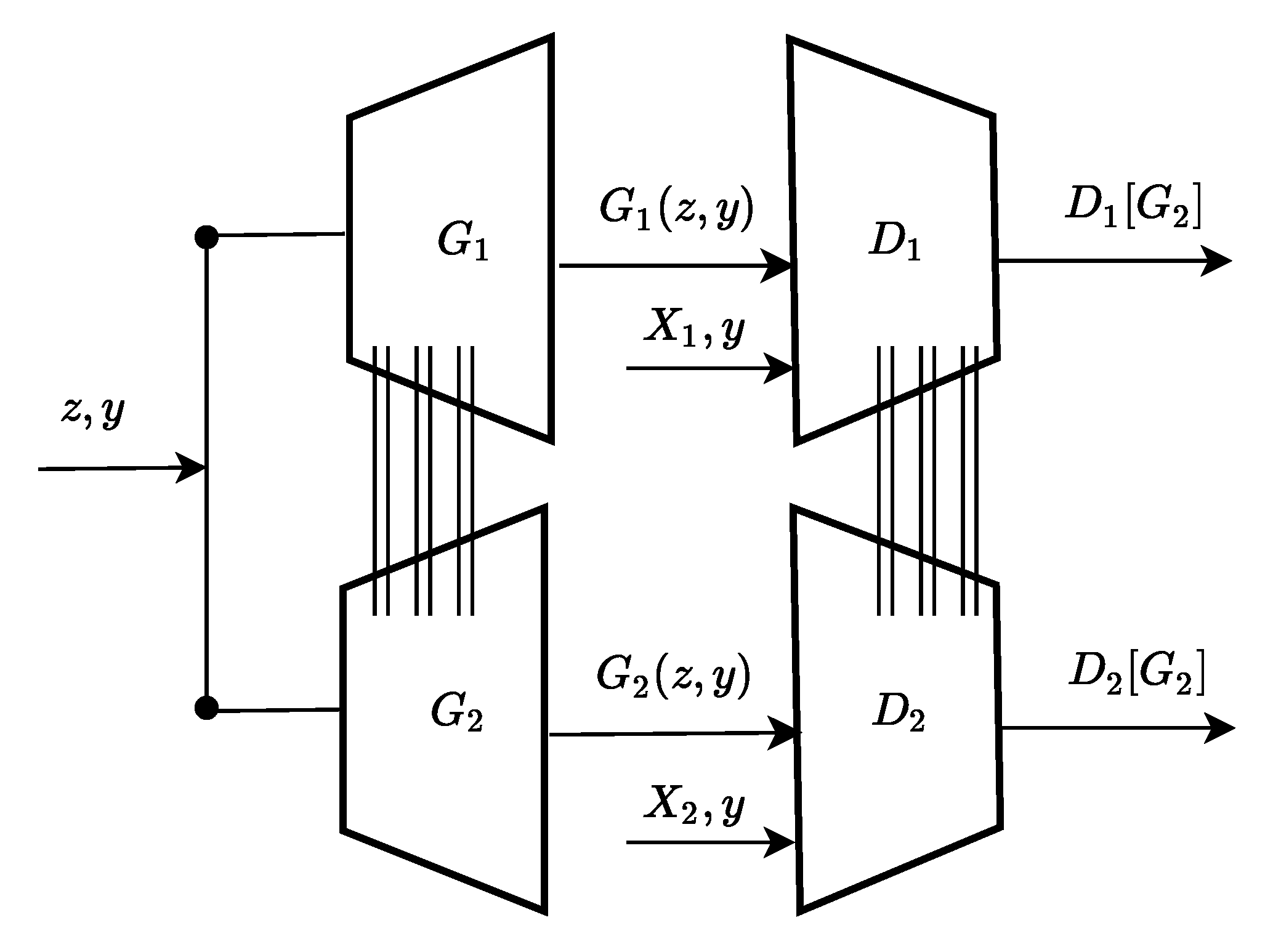
A schematic view of the RecommenderGAN model used the current work is presented in Figure 1. The generators (left) receive input latent vectors z and user segment y, and output matrices G1, G2. Discriminators (right) are trained alternatively with these artificial arrays and real samples X1, X2, and try to discern the difference. The error in this decision is backpropagated to update weights in the generators.
Architectural details of the network were settled upon after iterative experimentation and observation of results from different model design configurations and hyperparameter sets. Specifics of the layered configuration and dimensions of the final model appear in Table 1.
For the present dataset, more extensive (layer-wise) coupling of the weights within the generator networks proved necessary to obtain useful statistical results upon analysis. This is in contrast to the existing literature on coupled GANs, in which the main application domain is computer vision [17].
It was determined that the use of dropout layers [21] in improved convergence during training, but such layers had negligible positive effect when included in the discriminator sub-models.
The final model included a total of 326, 614, 406 parameters, of which 257, 407, 020 were trainable.
The optimization algorithm used for training the model was Adam (stochastic gradient descent), using default values for the configurable parameters (https://keras.io/api/optimizers/adam/).
2.3. Data Preparation
Electronic commerce dataset. The adversarially trained recommender model was developed using a dataset collected from an online retailer (https://www.kaggle.com/retailrocket/ecommerce-dataset). The dataset describes website visitors and their behaviors (view, “add” or buy items available for purchase); the attributes of these items; and a graph describing the hierarchy of categories to which each item belongs. Customers have been anonymized, identifiable only by a unique session number; all items, properties and categories were similarly hashed for confidentiality reasons.
The dataset comprises 2,756,101 behavioral events: (2,664,312 views, 69,332 “add to carts”, 22,457 purchases) observed on 1,407,580 distinct visitors. There are 417,053 unique items represented in the data.
Three different schemes for joint distribution learning can be constructed from the behaviors view, addtocart, and buy in the dataset—(view, add), (add, buy), and (view, buy). The (view, buy) scheme was studied here because it directly connects viewing a raw recommendation and a corresponding purchase.
User segmentation. In Reference [22], models of user engagement with digital services were developed based on metrics covering three aspects of observable variables: popularity, activity and loyalty. Each of these areas and metrics suggest means for grouping users in an implicit feedback situation.
In the current study, users were segmented based on counts of the number of interactions made within a session (this is referred to as “click depth” in Reference [22]). Each visitor/session in the dataset were assigned to one of five behavioral segments according to click depth, which increases in proportion to bin number. Visitor counts by segment for the (view, buy) scheme are summarized in Table 2.
Note that the first segment is empty in this table. User segmentation was based on the entire sample; for the (view, buy) group, no paired data fell into the lowest click depth count bin. (At least two actions are required to view and buy, and 86% of the entire sample comprised two or fewer interactions, and total buys less than 1%). The total sample size considered for the four segments was 10,591 visitors.
Compressed representation. The e-commerce dataset contained 417,053 distinct items in 1669 product categories. Data matrices covering the full-dimensional space () are prohibitively large for practical computation. This is exacerbated by the number of trainable parameters in the model (>257,000,000).
To address this cardinality issue, a compressed representation of the product data was created using an arithmetic coding algorithm [23]. For each visit, training data matrices were constructed having fixed dimensions of 1169 rows (one product category per row) and 300 columns (encoded bit strings representing items in corresponding category). This was the maximum encoded column dimension; for row encodings of lesser length, the bit string is prepended with zeros. The decoded result is identical regardless of length of this prefix; this is important in order to subsequently identify specific items recommended by the system.
The encoded, sparse data matrices profiling visitor behavior for Views (V) and Buys (B) can be expressed symbolically as:
where elements are indicator variables denoting whether a visitor interacts with category ‘m’ and item ‘n’, and (r = 1669 × c = 300) is the encoded matrix dimension.
GAN training is carried out in the compressed data space, and final recommendations are read out after decoding to the full column dimension of all items comprising the product catalog.
2.4. Evaluation Metrics
Assessments of recommendation systems in academic research often include utility statistics of the returned results (such as novelty, precision, sensitivity), or overall system computational efficiency [24,25,26]. To estimate the business value derived from deployed systems, effectiveness measures may be direct (conversion rates, click-through rates), or inferred (increased subscriptions, overall revenue lift, for example) [27].
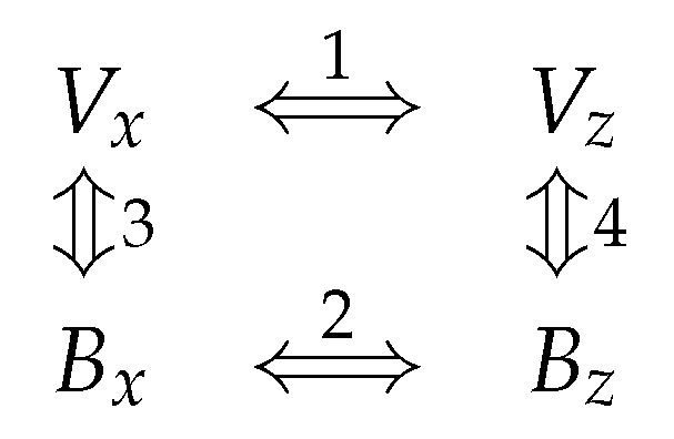
In the implicit feedback situation considered here, recommendations are created from sampling a joint distribution of behaviors. Consider the potential paths for system evaluation as suggested in Figure 2. In the left-hand column are the paired training data ; on the right, the generated recommendations .
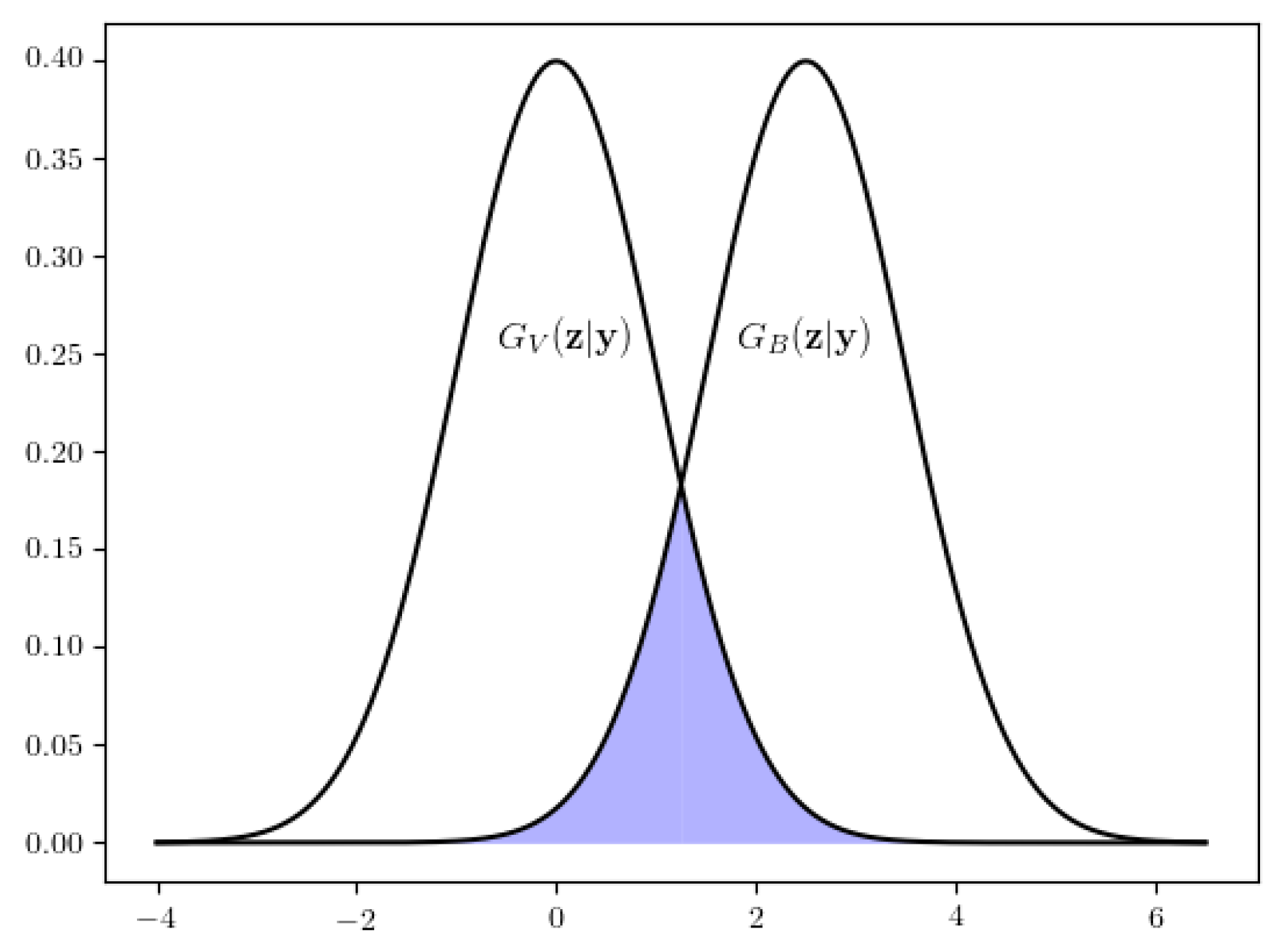
Without knowledge of the relevance of recommendations by human ratings or via purchasing behavior, evaluation in this preliminary work is based on objective metrics of similarity between the generated lists (path #4). Items contained in the intersection of generated recommendation sets are taken to signify the highest likelihood for completion of a transaction within the context of a given visitor session. This idea is illustrated in Figure 3.
Two metrics of evaluation are proposed:
- 1
- Specific items contained within the overlapping category sets that are both viewed and “bought”—a putative conversion rate;
- 2
- Coherence between categories in the paired recommendations.
Estimation of conversion rate is the most important statistic considered here; it is crucial for evaluation and optimization of recommender systems in terms of user utility, as well as for targeted advertising [28].
Category overlap is prerequisite to demonstration of the feasibility of the current approach to product recommendation.
Product conversion rate. Define the conversion rate as the number of items recommended and bought, to the count of all items recommended, conditioned on the set of overlapping product categories returned by the system:
where are items, are product categories, N is the number of GAN realizations, y denotes the user segment and “” denotes the cardinality of its argument. Note that in the current analysis, it is assumed that all recommended items are viewed by a visitor.
Category similarity. The average Jaccard similarity between recommended categories is given by
Training distribution statistics. Summary statistics comparing the distributions (Figure 2, path #1) are observed to provide qualitative information about the effectiveness of target distribution learning.
Null hypothesis tests. A legitimate question to ask upon analyzing the current results is this: “Are the generator realizations samples of the target joint distribution, or do they simply represent random noise?”.
To address this question, the analysis includes statistics estimated from simulation trials (n = 500) in which randomly selected elements from the (V, B) matrices are set equal to unit value, while maintaining the average sparsity observed in the decoded GAN predictions.
The random trials are meant to test the null hypothesis that there is no correlation between paired elements in the generator output.
The alternative hypothesis is that the recommendations contain relevant information that may provide utility to the system user.
2.5. Recommendation Experiments
Training. The system was trained on the encoded data for 1100 epochs, in randomly-selected batches of 16 examples each.
Statistics of training data for all networks comprising the model were observed during the training iterations.
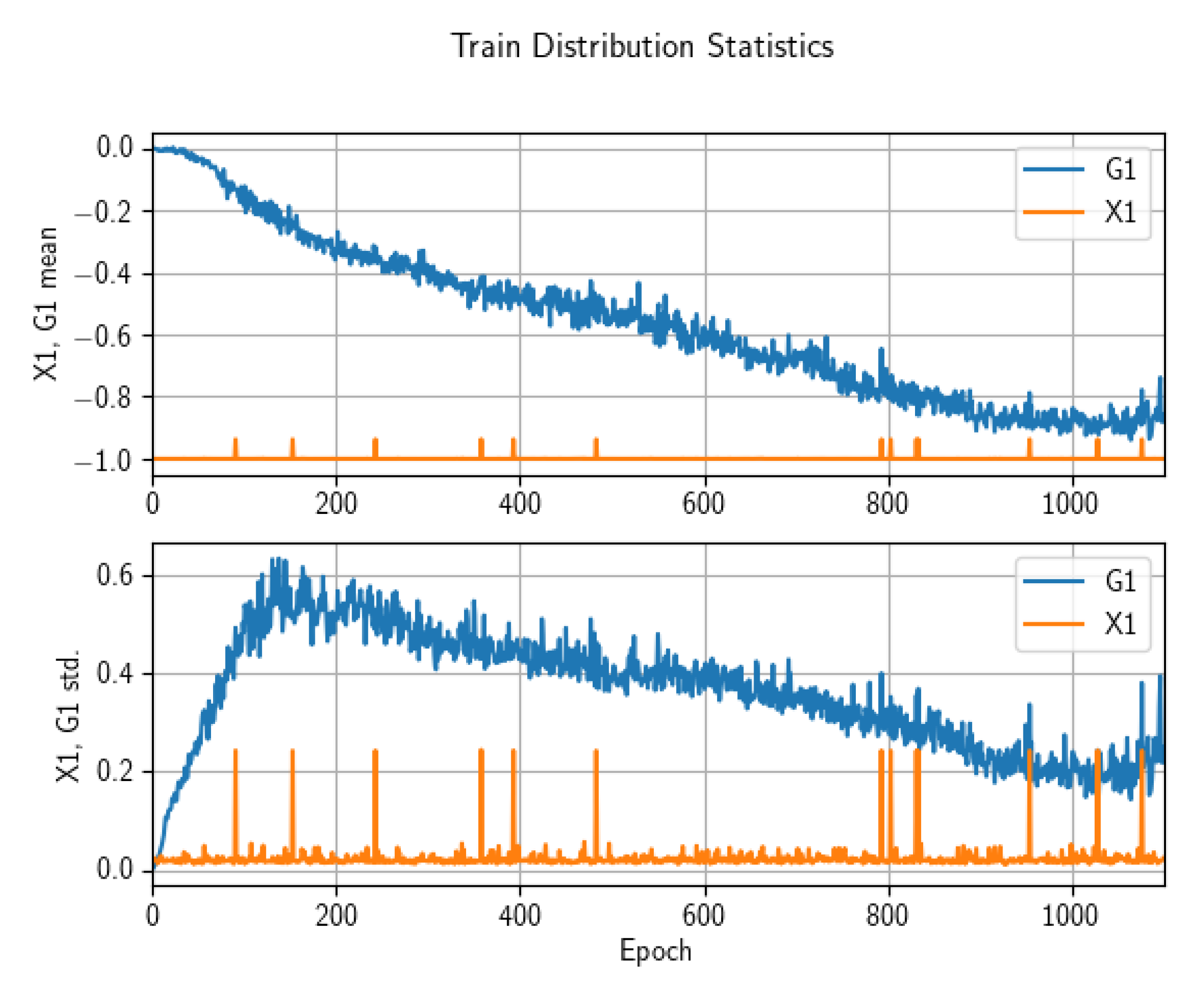
The statistics monotonically approached the true distribution those of the true until around epoch nunber 1110, at which point the GAN output began to diverge. One explanation for this may be that the representational capacity of the networks on this abstract learning task may have become exhausted [29]. Examples of this statistical evolution during training are shown in Figure 4. Note that training data matrix values were scaled onto the range [−1,+1], where the value “−1” corresponds to a zero valued element in the sparse raw data arrays.
Label smoothing on the positive ground truth examples presented to the discriminators was used to regularize the learning procedure [30].
At training stoppage, the observed discriminator accuracies where consistently in the ≈45–55% range, indicating that these models were unable to differentiate between the real and fake distributions produced by the generators [14].
Testing. Testing a machine learning model refers to evaluation of its output predictions obtained using out-of-sample (unseen) input data. This provides an estimate of the quality and generalization error of the model. Techniques such as cross-validation are often used to assess generalization potential. In contrast to many other learning algorithms, GANs do not have an objective function, rendering performance comparison of different models difficult [31].
For a concrete illustration, imagine that a GAN has been trained on a distribution of real images of human faces, and generates synthetic face samples after sufficient training iterations [32].
The degree to which the sampled distribution has learned to approximate the target distribution can be estimated by qualitative scoring; the assessment is subjectively accomplished by human observers, who easily measure how “facelike” these artificial faces appear to the eye.
Alternatively, objective metrics based on training and generated image data can be applied in some cases. Example objective metrics are proposed in Reference [31].
In the present application, the generated “images” are abstract representations of consumer activity, not concrete objects. An out-of-sample test in the conventional sense is not possible. The metrics of generative model performance and null hypothesis tests as described in Section 2.4 constitute the testing of the model developed in this work.
GAN predictions. After training, the model was stimulated with a noise vector and a user segment conditioning signal, producing a series of coupled predictions , as depicted in Figure 1. The discriminators serve only to guide training, and are disabled for the inference procedure.
A total of 2500 generation realizations was produced for each user segment. The recommendation matrices were decoded onto the full-dimensional space ( ) by the inverse arithmetic coding algorithm used in data preparation.
An sub-sample of these realizations was taken to compute key recommender evaluation metrics (Equations (4) and (5)). This was done because the decoding algorithm involves compute-intensive iteration, and is not amenable for computation on GPUs at this writing. Numerical optimization of the arithmetic decoding should be addressed in future extensions of this work.
The evaluation statistics were also calculated in null hypothesis tests, the results of which were averaged to obtain an estimate of the distribution expected under this hypothesis.
3. Results And Discussion
3.1. Main Statistical Results
The main experimental results of this paper are summarized in Table 3. CVR is the conversion rate (Equation (4)) and is the category similarity (Equation (5)). Here, y represents the user segment; are the predicted item and category counts, respectively. Row data in the table are averages over (1) 200 realizations from the GAN, and (2) 500 random trials (columns marked “rn”.)
The conversion rates (CVR) calculated from the GAN output range from 1.323 to 1.763%. The corresponding randomized values () are at least 3 orders of magnitude smaller. Based on this result, the null hypothesis of no relationship between paired samples in the generator output is rejected.
On this key statistical metric, the joint distribution of behaviors sampled from the trained GAN model is characterized by non-trivial signal to noise. The conversion rates observed from the sampled recommendations suggest utility of the system for consumers and digital retailers.
The category similarity for the randomized cases is around 50% for all user segments, while the GAN similarity is between 6.13% and 8.19%. The random procedure shows much greater similarity between recommended () and potential transactions–however given the negligible precision (), this similarity metric has negligible practical utility.
3.2. Benchmark Comparison Results
To place the current results into commercial context, experimental conversion rates were compared against benchmarks observed by digital retailers across industries and product types. In an online resource [33], conversion rates are estimated for 11 different industries and 9 product types. For a concise comparison, average values of these conversion rates are shown along with the mean GAN conversion rate obtained here. The data are summarized in Table 4.
It is seen from Table 4 that the GAN conversion rates are slightly less than, but on the order of, aggregated industrial and product type values. It is noted in Reference [33] that precise definitions of “conversion rate” may vary and the one used in this research may be slightly different than industrial convention. Nevertheless, the RecommenderGAN produces intriguing rates of conversion given the paucity of information about user segments that was used to develop this model.
3.3. Discussion
The results obtained from evaluation of the RecommenderGAN generated samples suggest that this approach may be useful for online recommendation systems. This section discusses difficulties with direct comparison to other deep models, identifies areas for improvement of the model presented in this preliminary work, and other assorted notes.
3.3.1. Comparison with Other Recommenders
A direct objective comparison of the present results with deep recommender systems found in the literature is problematic.
First, the present scheme lacks ground truth data with which to evaluate novel recommendations produced by the RecommenderGAN. This fact motivated the design of the evaluation metrics discussed in Section 2.4. GAN outputs are predictions that must ultimately be validated by human ratings of quality, or via offline methods such as A/B testing [34].
Secondly, the GAN outputs a distribution of evenly-weighted recommended items, not numeric ratings that could be used to compare against other algorithms using rank-based statistical metrics. Commonly used benchmarking datasets are based upon entities including user, item, rating and some attributes. In order to compare against other deep models directly, it would be necessary to either (i) refactor benchmark datasets from a rating scale for example, [1–5] for the MovieLens dataset [35]) onto the current binary-valued training data elements and re-interpret as a buy/no buy outcome, or vice versa (arbitrarily convert binary to a numeric scale). Such modification would shift the meaning of the data and the model, and it is not clear how to do this in a rigorously correct manner.
A qualitative comparison of the RecommenderGAN against selected deep recommendation models on the basis of their respective core algorithms, inputs and outputs is presented in Table 5.
3.3.2. Drawbacks of Current Method
Numerical efficiency. A limitation of the approach to recommendation as presented here is the numerical efficiency of the decoding process. The arithmetic coding algorithm used to decode the binary data matrices after training the model involves iteration and is not easily parallelizable. The dimensionality of the full catalog of products is extremely high; decoding compute times are consequently large. This mandates offline processing before deployment.
Future development should focus on numerical optimization of the decoding algorithm, to perhaps include compilation to another language, such as C++.
Ranking of recommendations. As discussed above, there is no ranking of recommendation results in the current scheme, as the GAN produces binary valued information upon decoding. Inherent filtering is accomplished by limiting the presented results to those contained within the category intersection set as seen in the operational definition of conversion rate (Equation (4)). This set is interpreted as representing the greatest likelihood for completing a transaction. On average over user segments, 13% of all categories are returned; of these, 0.46% of all catalog items are represented.
Conditioning signal. The current conditioning signal y is simply based on user dwell time. The information contained in this signal is relatively weak, as indicated by the variation of statistics across segments in Table 3. It is reasonable to anticipate more stringent filtering, and consequent precision and relevance of results, upon the introduction of more robust demographic or behavioral data in the conditioning signal input to the model. This would facilitate a more personalized recommendation experience. The model architecture considered here directly supports such segmentation, and is an important topic to be explored in extensions to this research.
3.3.3. General Discussion Points
Selection bias and scalability. The estimation of conversion rates is difficult due to two related, key issues: training sample selection bias and data sparsity [28]. Sample selection bias refers to discrepancies in data distribution between model training and inference in conventional recommenders—that is, training data often comprise only “clicked” samples, while inference is made on all impression samples. Selection bias is said to limit the accuracy of inference assuming the user proceeds through the sequence [28]. As examples are a small fraction of , a highly imbalanced training set results, biased towards sparse positive examples [36].
This issue is partially avoided in the present research, where the training data are constructed from all items, extracted from the user sequence . Model recommendations are produced on items having semantic correspondence to the first and third actions in this sequence (Note: Selection bias is not limited to implicit recommendation systems. Evaluating the performance of online recommenders with user feedback is biased towards the selectively recommend items [37]).
Intertwined with the data sparsity situation in implicit recommendation is the issue of scalability. In collaborative filtering algorithms, the consideration of all paired user-item data points as input to a model is infeasible; the numbers of those pairs can be exceedingly large, and as noted, each user provides feedback on a very small fraction of the available items [36].
The present system provides scalability to the full product catalog (417,053 items) by virtue of the arithmetic coding compression scheme, albeit at the cost of numerical performance upon decoding.
An open question. Has the true joint distribution been learned? Making inferences about the joint distribution of viewing and buying behavior to inform marketing decisions is the motivation behind this analysis. Investigators have previously shown that GANs may not adequately approximate the target distribution, as the support of the generated distribution was low due to so-called mode collapse [38], where the generator learns to mimic certain modes in the training data in order to trick the discriminator during training.
It is debatable whether or not mode collapse is an issue in the present problem formulation, given the abstract formulation of the problem using binary indicator matrices to represent consumer behavior. This is an open question that may be addressed in further research.
4. Conclusions
We have shown that a coupled, conditional generative adversarial network can learn to generate samples from the joint distribution of online user behavior inferred from () item pairs. These samples can be used to make product recommendations for specific user segments.
Our results are preliminary, however they suggest that the recommendations produced by the model may provide utility for consumers and digital retailers.
Conversion rate statistics computed from the trained GAN output samples ranged from 1.323 to 1.763%. These statistics were shown to be significant in comparison to null hypothesis testing results. This suggests that the GAN recommendations may provide utility for consumers and digital retailers.
A comparison of GAN-predicted conversion rates against benchmarks from digital retailers representing many industries and product types showed the GAN conversion rates to approximate these aggregated commercial rates.
The capacity of the system scales to the full item catalog dimension (417,053 items) by the use of an arithmetic coding compression algorithm.
A number of original aspects of the approach to recommendation advanced in this research can be identified. These include—(i) Direct modeling of the joint distribution between product views and buys for a user segment; (ii) I/O: Inputs to the trained generative model are user segment and noise vectors; the outputs are matrices of coupled (view, buy) predictions; (iii) Coverage of complete product catalogs can be represented in each generated distribution; (iv) Application of a linear encoding algorithm to very high-dimensional data vectors, enabling computation and ultimate decoding to product space; (v) A focus on transaction (versus user rating) for recommended products by design.
In future development of our model, a means for objective comparison against competitive recommendation algorithms should be prioritzed. Such comparison should be carried out following a systematic methodology as described in Reference [39]. This would require the articulation of a strategy for reconciling the (presently) binary-valued GAN outputs with numeric ratings in common usage with other recommendation algorithms. In addition, work is needed to improve the numerical performance of the decoding algorithm used to invert to product space.
Author Contributions
Concept, methods, analysis J.R.B.; writing J.R.B. and A.M. All authors have read and agreed to the published version of the manuscript.
Funding
This research received no external funding.
Conflicts of Interest
The authors declare no conflict of interest.
Abbreviations
The following abbreviations are used in this manuscript:
| GAN | Generative adversarial network |
| CVR | Conversion rate |
| NCF | Neural collaborative filtering |
| MLP | Multilayer perceptron |
| RNN | Recurrent neural network |
References
- Gilula, Z.; McCulloch, R.; Ross, P. A direct approach to data fusion. J. Mark. Res. 2006, XLIII, 73–83. [Google Scholar] [CrossRef]
- Anderson, C. The Long Tail: Why the Future of Business Is Selling Less of More; Hyperion Press: New York, NY, USA, 2006. [Google Scholar]
- MacKenzie, I.; Meyer, C.; Noble, S. How Retailers Can Keep Up with Consumers. 2013. Available online: Https://mck.co/2fGI7Vj (accessed on 9 June 2019).
- Gomez-Uribe, C.; Hunt, N. The Netflix Recommender System: Algorithms, Business Value, and Innovation. ACM Trans. Manag. Inf. Syst. 2015, 6, 1–19. [Google Scholar] [CrossRef] [Green Version]
- Iyengar, S.; Lepper, M. When Choice is Demotivating: Can One Desire Too Much of a Good Thing? J. Personal. Soc. Psychol. 2001, 79, 995–1006. [Google Scholar] [CrossRef]
- Batmaz, Z.; Yurekli, A.I.; Bilge, A.; Kaleli, C. A review on deep learning for recommender systems: Challenges and remedies. Artif. Intell. Rev. 2018, 52, 1–37. [Google Scholar] [CrossRef]
- Zhang, S.; Yao, L.; Sun, A. Deep Learning Based Recommender System: A Survey and New Perspectives. ACM Comput. Surv. 2019, 52, 1–38. [Google Scholar] [CrossRef] [Green Version]
- Brand, M. Fast online SVD revisions for lightweight recommender systems. In Proceedings of the SIAM International Conference on Data Mining, San Francisco, CA, USA, 1–3 May 2003. [Google Scholar]
- He, X.; Liao, L.; Zhang, H.; Nie, L.; Hu, X.; Chua, T. Neural Collaborative Filtering. In Proceedings of the 26th International Conference on World Wide Web, Perth, Australia, 3–7 April 2017. [Google Scholar]
- Sedhain, S.; Menon, A.K.; Sanner, S.; Xie, L. AutoRec: Autoencoders Meet Collaborative Filtering. In Proceedings of the 24th International Conference on World Wide Web, Florence, Italy, May 2015. [Google Scholar]
- Hidasi, B.; Karatzoglou, A.; Baltrunas, L.; Tikk, D. Session-based Recommendations with Recurrent Neural Networks. arXiv, 2015; arXiv:1511.06939. [Google Scholar]
- Ying, R.; He, R.; Chen, K.; Eksombatchai, P.; Hamilton, W.L.; Leskovec, J. Graph Convolutional Neural Networks for Web-Scale Recommender Systems. In Proceedings of the 24th ACM SIGKDD International Conference on Knowledge Discovery & Data Mining, London, UK, 19–23 August 2018. [Google Scholar] [CrossRef] [Green Version]
- Yoo, J.; Ha, H.; Yi, J.; Ryu, J.; Kim, C.; Ha, J.; Kim, Y.; Yoon, S. Energy-Based Sequence GANs for Recommendation and Their Connection to Imitation Learning. arXiv, 2017; arXiv:1706.09200. [Google Scholar]
- Goodfellow, I.J.; Pouget-Abadie, J.; Mirza, M.; Xu, B.; Warde-Farley, D.; Ozair, S.; Courville, A.; Bengio, Y. Generative Adversarial Networks. arXiv, 2014; arXiv:1406.2661. [Google Scholar]
- Mirza, M.; Osindero, S. Conditional Generative Adversarial Nets. arXiv, 2014; arXiv:1411.1784. [Google Scholar]
- Gauthier, J. Conditional generative adversarial nets for convolutional face generation. Cl. Proj. Stanf. CS231N Convol. Neural Netw. Vis. Recognit. 2014, 2014, 2. [Google Scholar]
- Liu, M.Y.; Tuzel, O. Coupled Generative Adversarial Networks. In Advances in Neural Information Processing Systems 29; Lee, D.D., Sugiyama, M., Luxburg, U.V., Guyon, I., Garnett, R., Eds.; Curran Associates, Inc.: Red Hook, NY, USA, 2016; pp. 469–477. [Google Scholar]
- Abadi, M.; Barham, P.; Chen, J.; Chen, Z.; Davis, A.; Dean, J.; Devin, M.; Ghemawat, S.; Irving, G.; Isard, M.; et al. TensorFlow: A system for large-scale machine learning. In Proceedings of the 12th USENIX Symposium on Operating Systems Design and Implementation (OSDI 16), Savannah, GA, USA, 2–4 November 2016; pp. 265–283. [Google Scholar]
- Chollet, F. Keras. 2015. Available online: https://keras.io (accessed on 31 August 2020).
- Linder-Norén, E. Keras-GAN: Keras Implementations of Generative Adversarial Networks. 2018. Available online: https://github.com/eriklindernoren/Keras-GAN (accessed on 31 August 2020).
- Srivastava, N.; Hinton, G.; Krizhevsky, A.; Sutskever, I.; Salakhutdinov, R. Dropout: A Simple Way to Prevent Neural Networks from Overfitting. J. Mach. Learn. Res. 2014, 15, 1929–1958. [Google Scholar]
- Lehmann, J.; Lalmas, M.; Yom-Tov, E.; Dupret, G. Models of User Engagement. In UMAP’12-Proceedings of the 20th International Conference on User Modeling, Adaptation, and Personalization; Springer: Berlin/Heidelberg, Germany, 2012; pp. 164–175. [Google Scholar] [CrossRef]
- MacKay, D. Information Theory, Inference, and Learning Algorithms; Cambridge University Press: Cambridge, UK, 2003. [Google Scholar]
- McNee, S.M.; Riedl, J.; Konstan, J.A. Being accurate is not enough: How accuracy metrics have hurt recommender systems. In Proceedings of the CHI Extended Abstracts on Human Factors in Computing Systems, Montréal, QC, Canada, 22–27 April 2006. [Google Scholar]
- Castells, P.; Vargas, S.; Wang, J. Novelty and Diversity Metrics for Recommender Systems: Choice, Discovery and Relevance. In Proceedings of the International Workshop on Diversity in Document Retrieval (DDR-2011), Dublin, Ireland, April 2011. [Google Scholar]
- Koren, Y. Factorization meets the neighborhood: A multifaceted collaborative filtering model. In Proceedings of the 14th ACM SIGKDD International Conference on Knowledge Discovery and Data Mining, Las Vegas, NV, USA, 24–27 August 2008; pp. 426–434. [Google Scholar] [CrossRef]
- Jannach, D.; Jugovac, M. Measuring the Business Value of Recommender Systems. ACM Trans. Manag. Inf. Syst. 2019, 10, 1–23. [Google Scholar] [CrossRef] [Green Version]
- Wen, H.; Zhang, J.; Wang, Y.; Bao, W.; Lin, Q.; Yang, K. Conversion Rate Prediction via Post-Click Behaviour Modeling. arXiv, 2019; arXiv:cs.LG/1910.07099. [Google Scholar]
- Bermeitinger, B.; Hrycej, T.; Handschuh, S. Representational Capacity of Deep Neural Networks—A Computing Study. arXiv, 2019; arXiv:1907.08475. [Google Scholar]
- Szegedy, C.; Vanhoucke, V.; Ioffe, S.; Shlens, J.; Wojna, Z. Rethinking the Inception Architecture for Computer Vision. In Proceedings of the IEEE Conference on Computer Vision and Pattern Recognition, Boston, MA, USA, 7–12 June 2015. [Google Scholar]
- Salimans, T.; Goodfellow, I.; Zaremba, W.; Cheung, V.; Radford, A.; Chen, X.; Chen, X. Improved Techniques for Training GANs. In Advances in Neural Information Processing Systems 29; Lee, D.D., Sugiyama, M., Luxburg, U.V., Guyon, I., Garnett, R., Eds.; Curran Associates, Inc.: Red Hook, NY, USA, 2016; pp. 2234–2242. [Google Scholar]
- Karras, T.; Aila, T.; Laine, S.; Lehtinen, J. Progressive Growing of GANs for Improved Quality, Stability, and Variation. arXiv, 2017; arXiv:1710.10196. [Google Scholar]
- Ogonowski, P. 15 Ecommerce Conversion Rate Statistics. 2020. Available online: https://www.growcode.com/blog/ecommerce-conversion-rate (accessed on 6 April 2020).
- Gilotte, A.; Calauzènes, C.; Nedelec, T.; Abraham, A.; Dollé, S. Offline A/B Testing for Recommender Systems. In Proceedings of the Eleventh ACM International Conference on Web Search and Data Mining-WSDM ’18, Marina Del Rey, CA, USA, 5–9 February 2018. [Google Scholar]
- Harper, F.M.; Konstan, J. The MovieLens datasets: History and context. ACM Trans. Interact. Intell. Syst. 2015, 5, 1–19. [Google Scholar] [CrossRef]
- Hu, Y.; Koren, Y.; Volinsky, C. Collaborative filtering for implicit feedback datasets. In Proceedings of the IEEE International Conference on Data Mining (ICDM 2008), Pisa, Italy, 15–19 December 2008; pp. 263–272. [Google Scholar]
- Yang, L.; Cui, Y.; Xuan, Y.; Wang, C.; Belongie, S.; Estrin, D. Unbiased Offline Recommender Evaluation for Missing-Not-At-Random Implicit Feedback. In Proceedings of the Twelfth ACM Conference on Recommender Systems (RecSys ‘18), Vancouver, BC, Canada, 2–7 October 2018. [Google Scholar]
- Arora, S.; Zhang, Y. Do GANs actually learn the distribution? An empirical study. arXiv, 2017; arXiv:1706.08224. [Google Scholar]
- Dacrema, M.F.; Boglio, S.; Cremonesi, P.; Jannach, D. A Troubling Analysis of Reproducibility and Progress in Recommender Systems Research. arXiv, 2019; arXiv:1911.07698. [Google Scholar]
Figure 1.
Coupled, conditional RecommenderGAN architecture. All component networks are active during training. Samples from the trained model are generated by presenting latent vector z and user segment y to the generators .
Figure 1.
Coupled, conditional RecommenderGAN architecture. All component networks are active during training. Samples from the trained model are generated by presenting latent vector z and user segment y to the generators .

Figure 2.
Evaluation routes for generative adversarial network (GAN) recommender.

Figure 3.
Recommended items are drawn from intersection of outputs generated by the trained GAN, indicated in blue. and ’ are the view and buy distributions, respectively.
Figure 3.
Recommended items are drawn from intersection of outputs generated by the trained GAN, indicated in blue. and ’ are the view and buy distributions, respectively.

Figure 4.
Batch statistics for and versus training epoch. Similar statistic values were observed for , . Batch size = 16.
Figure 4.
Batch statistics for and versus training epoch. Similar statistic values were observed for , . Batch size = 16.


Table 1.
Configuration details for discriminators (left) and generators (right). The “?” symbol indicates batch size of the associated tensor. Weights are shared between layers D:(9–14) and G:(6–13).
Table 1.
Configuration details for discriminators (left) and generators (right). The “?” symbol indicates batch size of the associated tensor. Weights are shared between layers D:(9–14) and G:(6–13).
| ID | D Layer | Output Size | ID | G Layer | Output Size |
|---|---|---|---|---|---|
| 1 | Input (y) | (?,1) | 1 | Input (y) | (?,1) |
| 2 | Embedding | (?,1,500700) | 2 | Embedding | (?,1,100) |
| 3 | Flatten | (?,500700) | 3 | Flatten | (?,100) |
| 4 | Reshape | (?,1669,300,1) | 4 | Input (z) | (?,100) |
| 5 | Input (X) | (?,1669,300,1) | 5 | Multiply (3,4) | (?,100) |
| 6 | Multiply (4,5) | (?,1669,300,1) | 6,7 | Dense, ReLU | (?,128) |
| 7 | AvgPooling | (?,834,15,1) | 8 | BatchNorm. | (?,128) |
| 8 | Flatten | (?,125100) | 9 | Dropout | (?,128) |
| 9,10 | Dense, ReLU | (?,512) | 10,11 | Dense, ReLU | (?,256) |
| 11,12 | Dense, ReLU | (?,256) | 12 | BatchNorm. | (?,256) |
| 13,14 | Dense, ReLU | (?,64) | 13 | Dropout | (?,256) |
| 15 | Dense | (?,1) | 14 | Dense | (?,500700) |
| 15 | Reshape | (?,1669,300,1) |
Table 2.
Visitor counts by segment for scheme (view, buy).
| Segment | 0 | 1 | 2 | 3 | 4 |
|---|---|---|---|---|---|
| Count | n/a | 309 | 1182 | 1510 | 7590 |
Table 3.
Average conversion rate and category similarity by segment.
| y | #I | #C | CVR | CVRrn | Jc | |
|---|---|---|---|---|---|---|
| 1 | 1648 | 239 | 1.763 | 0.0005 | 8.19 | 50.66 |
| 2 | 2037 | 213 | 1.414 | 0.0004 | 7.37 | 51.36 |
| 3 | 2522 | 190 | 1.323 | 0.0005 | 6.13 | 50.04 |
| 4 | 1419 | 222 | 1.644 | 0.0004 | 7.57 | 50.81 |
Table 4.
Experimental conversion rate compared to selected industrial average benchmarks. GAN: current results, segment-wise average; Industry: average over 11 industrial markets; Product: average of 9 product types [33].
Table 4.
Experimental conversion rate compared to selected industrial average benchmarks. GAN: current results, segment-wise average; Industry: average over 11 industrial markets; Product: average of 9 product types [33].
| GAN | Industry | Product |
|---|---|---|
| 1.536 | 2.089 | 1.827 |
Table 5.
Comparison of present model and selected deep recommenders.
| Algorithm | Reference | Recommender Input | Recommender Output |
|---|---|---|---|
| MLP+Matrix factorization | He et al. [9] | User, item vectors | Item ratings |
| Autoencoder | Sedhain et al. [10] | User, item vectors | Item ratings |
| Recurrent neural network | Hidasi et al. [11] | Item sequence | Next item |
| Graph neural network | Ying et al. [12] | Item/feature graph | Top items |
| Sequence GAN | Yoo et al. [13] | Item sequence | Next item |
| RecommenderGAN | This work | Noise, user vectors | View, buy matrices |
© 2020 by the authors. Licensee MDPI, Basel, Switzerland. This article is an open access article distributed under the terms and conditions of the Creative Commons Attribution (CC BY) license (http://creativecommons.org/licenses/by/4.0/).
Share and Cite
MDPI and ACS Style
Bock, J.R.; Maewal, A. Adversarial Learning for Product Recommendation. AI 2020, 1, 376-388. https://0-doi-org.brum.beds.ac.uk/10.3390/ai1030025
AMA Style
Bock JR, Maewal A. Adversarial Learning for Product Recommendation. AI. 2020; 1(3):376-388. https://0-doi-org.brum.beds.ac.uk/10.3390/ai1030025
Chicago/Turabian StyleBock, Joel R., and Akhilesh Maewal. 2020. "Adversarial Learning for Product Recommendation" AI 1, no. 3: 376-388. https://0-doi-org.brum.beds.ac.uk/10.3390/ai1030025