A Neurally Inspired Model of Figure Ground Organization with Local and Global Cues


Department of Electrical and Computer Engineering, Johns Hopkins University, Baltimore, MD 21218, USA
AI 2020, 1(4), 436-464; https://0-doi-org.brum.beds.ac.uk/10.3390/ai1040028
Submission received: 31 August 2020
/
Revised: 21 September 2020
/
Accepted: 29 September 2020
/
Published: 6 October 2020
(This article belongs to the Section AI Systems: Theory and Applications)
Abstract
:Figure Ground Organization (FGO)-inferring spatial depth ordering of objects in a visual scene-involves determining which side of an occlusion boundary is figure (closer to the observer) and which is ground (further away from the observer). A combination of global cues, like convexity, and local cues, like T-junctions are involved in this process. A biologically motivated, feed forward computational model of FGO incorporating convexity, surroundedness, parallelism as global cues and spectral anisotropy (SA), T-junctions as local cues is presented. While SA is computed in a biologically plausible manner, the inclusion of T-Junctions is biologically motivated. The model consists of three independent feature channels, Color, Intensity and Orientation, but SA and T-Junctions are introduced only in the Orientation channel as these properties are specific to that feature of objects. The effect of adding each local cue independently and both of them simultaneously to the model with no local cues is studied. Model performance is evaluated based on figure-ground classification accuracy (FGCA) at every border location using the BSDS 300 figure-ground dataset. Each local cue, when added alone, gives statistically significant improvement in the FGCA of the model suggesting its usefulness as an independent FGO cue. The model with both local cues achieves higher FGCA than the models with individual cues, indicating SA and T-Junctions are not mutually contradictory. Compared to the model with no local cues, the feed-forward model with both local cues achieves % improvement in terms of FGCA.
1. Introduction
An important step in the visual processing hierarchy is putting together fragments of features into coherent objects and inferring the spatial relationship between them. The feature fragments can be based on color, orientation, texture, and so forth. Grouping [1,2] refers to the mechanism by which the feature fragments are put together to form perceptual objects. Such objects in the real world may be isolated, fully occluding one another or partially occluding, depending on the observer’s viewpoint. In the context of partially occluding objects, Figure-ground organization (FGO) refers to determining which side of an occlusion boundary is the occluder, closer to the observer, referred to as figure and which side is the occluded, far away from the observer, termed as ground.
Gestalt psychologists have identified a variety of cues that mediate the process of FGO [3]. Based on the spatial extent of information integration, these cues can be classified into local and global cues. Global cues such as symmetry [4], surroundedness [5], and size [6] of regions integrate information over a large spatial extent to determine figure-ground relationship between objects. Local cues, on the other hand, achieve the same by analysis of only a small neighborhood near the boundary of an object. Hence, they are particularly attractive from a computational standpoint. Some examples of local cues are T-junctions [7] and shading [8], including extremal edges [9,10].
The neural mechanism by which FGO is achieved in the visual cortex is an active area of research, referred to as Border Ownership (BO) coding. The contour fragments forming an object’s boundary are detected by Simple and Complex cells in the area V1 of primate visual cortex with their highly localized, retinotopically organized receptive fields. Cells in area V2, which receive input from V1 Complex cells, were found to code for BO by preferentially firing at a higher rate when the figural object was located on the preferred side of the BO coding neuron at its preferred orientation, irrespective of local contrast [11]. Recently, Williford and von der Heydt [12], remarkably show for the first time, that V2 neurons maintain the same BO preference properties even for objects in complex natural scenes.
Many computational models [13,14,15] have been proposed to explain the neural mechanism by which FGO or BO coding is achieved in the visual cortex. Based on the connection mechanism, those models can be classified as feed-forward, feedback [16,17] or lateral interaction models [15]. In this work, a neurally motivated, feed-forward computational model of FGO incorporating both local and global cues is presented. While exactly mimicking the neural processing at every step is not attempted, an attempt to keep it as biologically motivated as possible is made.
The FGO model developed here has three independent feature channels, Color, Intensity and Orientation. The main computational construct of the model is a BO computation mechanism that embodies Gestalt principles of convexity, surroundedness and parallelism, which is identical to all feature channels. In addition, many additional modifications are introduced to make it suitable for performing FGO and to incorporate local cues, as detailed in Section 3. The model, applicable to any natural image, is tested on the widely used BSDS figure-ground dataset. First, it is shown that even the model with only global cues, devoid of any local cues achieves good results on the BSDS figure-ground dataset. Let us call this the Reference model, against which the performance of models with added local cues is compared.
Two local cues are added to the Reference model: Spectral Anisotropy [10,18,19] and T-Junctions. Spectral Anisotropy (SA) is the presence of anisotropy in the oriented high frequency spectral power in a local region around the occlusion boundary, only on the figure side, but absent of the background side, which was established in a data-driven manner in [10,19,20]. In other words, SA is the presence of orthogonal high frequency spectral power on figure side that far exceeds the parallel power on the same side with respect to object boundary, but no such anisotropic distribution on the background side. This anisotropic distribution can arise from texture compression and shading gradients on the figure side because of the surface curvature of the foreground object. The usefulness of such texture and shading gradients on the foreground side as a local figure-ground cue was first observed through rigorous psychophysics experiments of Palmer and Ghose [9,21,22]. T-Junctions are formed when the the boundary of an occluding surface intersects with that of an occluded surface [23]. It is the location in an image where three different surfaces with different luminances abut each other [24]. The contour that looks “obstructed” by the occluding contour forms the “stem” of the T-Junction, whereas the occluding contour (always owned by the figure) forms the “hat” of the T-Junction. For a deeper understanding of T-Junctions and the role they play in figure-ground organization, readers are encouraged to refer to Wagemans et al. [1].
The motivation behind adding local cues is their relatively low computational cost compared to global cues. Spectral Anisotropy (SA) was shown to be a valid cue for FGO [10,18,19] in predicting which side of an occlusion boundary is figure and which the background. Moreover, SA can be computed efficiently in a biologically plausible (See Section 4.1) manner using convolutions, making it an attractive candidate. T-Junctions are commonly viewed as one of the strongest cues of occlusion and their computation can be explained on the basis of end-stopped cells [7,25,26]. This is the biological motivation to incorporate them into the model.
There are only two local cues in the model. Both local cues influence the Orientation channel only as the properties they capture are more closely related to this feature. Certainly, many more local cues and global cues would be needed for best performance in real world images. But, here the primary motivation is to develop a common computational framework and investigate how these local and global cues can be incorporated into a model of FGO. Second, the purpose of this work is to verify whether local cues can co-exist along with the global cues. If so, how useful are these local cues? Can they lead to a statistically significant improvement in the model’s performance when added alone? Finally, are these local cues mutually facilitatory leading to even further improvement, when added together? For these purposes, the minimalistic model with few global cues and even fewer local cues added to only one of the three feature channels provides an excellent analysis framework. The goal of this work is to study, from first principles, the effect of local and global cues in FGO, not necessarily to build a model with best performance. However, the performance of the model is compared with state-of-the-art models of FGO, which are not biologically motivated, and show that this model performs competitively.
2. Related Work
FGO has been an active area of research in Psychology since nearly a century [27] ago. The Gestalt principles of FGO and grouping such as common fate, symmetry, good continuation, similarity and so forth were formulated by Max Wertheimer [28] along with Kurt Koffka [3] and many others. Excellent reviews about the Gestalt principles of FGO and grouping can be found in References [1,2]. It is an active area of research in neuroscience [11,29,30,31] and computer vision [32,33,34] as well. The literature review is limited to computational models only. Even though the terms “FGO”, “BO” or “grouping” are not used in many publications that were reviewed, the common goal in all of them is related to inferring depth ordering of objects.
A local shapeme based model employing Conditional Random Fields (CRF) to enforce global consistency at T-junctions was proposed in References [32]. Hoiem et al. [33,35] used a variety of local region, boundary, Gestalt and depth based cues in a CRF model to enforce consistency between boundary and surface labels. An optimization framework [36] to obtain a 2.1D sketch by constraining the “hat” of the T-junction to be figure and “stem” to be ground was proposed, which uses human labeled contours and T-junctions. In an extension [37], a reformulated optimization over regions, instead of pixels, was proposed. By using various cues such as, curve and junction potentials, convexity, lower-region, fold/cut and parallelism, Leichter and Lindenbaum [38] train a CRF model to enforce global consistency. In a series of papers Palou and Salembier [39], Palou and Salembier [40], Palou and Salembier [41] show how image segmentation and depth ordering (FGO) can be performed using only low-level cues. Their model uses Binary Partition Trees (BPT) [42] for hierarchically representing regions of an image, performs depth ordering by iteratively pruning the branches of BPT enforcing constraints based on T-junctions and other depth related cues. In a recent work [34], which uses Structured Random Forests (SRF) for boundary detection, simultaneous boundary detection and figure-ground labeling is performed. They use shape cues, extremal edge basis functions [10], closure, image torque [43] and so forth to train the SRFs.
Yu et al. [44] present a hierarchical Markov Random Field (MRF) model incorporating rules for continuity of depth on surfaces, discontinuity at edges between surfaces and local cues such as T- and L-junctions. The model learns from a couple examples and effectively does depth segregation, thereby FGO. In Reference [45], a neurally plausible model integrating multiple figure-ground cues using belief propagation in Bayesian networks with leaky integrate and fire neurons was proposed. A simultaneous segmentation and figure-ground labeling algorithm was reported in Reference [46] which uses Angular Embedding [47] to influence segmentation cues from figure-ground cues and vice-versa. Similar attempts with primary goal of segmenting images and labeling object classes using figure-ground cues can be seen in References [48,49].
Differentiation/Integration for Surface Completion (DISC) model [50] was proposed in which BO is computed by detecting local occlusion cues such as T- and L- junctions and comparing non-junction border locations with junction locations for BO consistency with the local cues. A Bayesian belief network based model was proposed [51] in which local cues (curvature and T-junctions) interact with medial axis or skeleton of the shape to determine BO.
In one of the early attempts [52], a two layer network with connections between “computational units” within and across layers is proposed. These units integrate bottom-up edge input with top-down attention input to realize FGO. Grossberg and Mingolla [53], Grossberg [54] propose that a reciprocal interaction between a Boundary Contour System (BCS) extracting edges and a Feature Contour System (FCS) extracting surfaces achieves not only FGO, but also 3D perception. A model of contour grouping and FGO was proposed in Reference [25] central to which is a “grouping” mechanism. The model not only generates figure-ground labels, but also simulates the perception of illusory contours. Another influential model was proposed in Reference [55] with feedback and feed-forward connections having 8 different computational modules to obtain representations of contours, surfaces and depth. Roelfsema et al. [14], Jehee et al. [56] propose multilayer feedback networks resembling the neural connection pattern in the visual cortex to perform BO assignment through feedback from higher areas. Li Zhaoping et al. [57,58] propose a model of FGO based on V1 mechanisms. The model consists of orientation selective V1 neurons which influence surrounding neurons through mono-synaptic excitatory and di-synaptic suppressive connections. The excitatory lateral connections mimic colinear excitation [59] and cross-orientation facilitation [60], while inhibitory connections model the iso-orientation suppression [61]. In a related model [15], neurons in V2 having properties of convexity preference, good continuation and proximity was presented. A BO coding model which detects curvatures, L-Junctions and sends proportional signals to a BO layer was proposed by Kikuchi and Akashi [62], where BO signals are propagated along the contour for two sides of BO.
The model proposed by Craft et al. [13] consists of edge selective cells, BO cells and multi-scale grouping (G) cells. The G cells send excitatory feedback to those BO cells that are co-circular and point to the center of the annular G cell receptive field. The model incorporates Gestalt principles of convexity, proximity and closure. But, it is a feedback model tested only on simple geometric shapes, not real-world natural images. Several models [16,63,64,65] with similar computational mechanisms have been proposed to explain various phenomena related to FGO, saliency, spatial attention, and so forth. A model akin to Reference [13] was proposed in Reference [66], where in addition to G cells the model consists of region cells at multiple scales. In a feedback model [67] based on the interaction between dorsal and ventral streams, surfaces which are of smaller size, greater contrast, convex, closed, having higher spatial frequency are preferentially determined as figures. The model also accounts for figure-ground cues such as lower region and top-bottom polarity. In a series of papers [68,69,70] Sakai and colleagues formulate a BO model in which localized, asymmetric surround modulation is used to detect contrast imbalance, which then leads to FGO. Russell et al. [63] propose a feed-forward model with Grouping and Border Ownership cells to study proto-object based saliency. Though the proposed model is inspired by this work, the goal of Russell et al. [63] model is to explain the formation of proto-objects [71] and saliency prediction, not Figure-Ground Organization. Another related model is proposed by Hu et al. [17], which is a recurrent model with feedback connections, devoid of any local cues. To the best of our knowledge this work is the first feed-forward model of FGO with both local and global cues. Also, this the the first such model tested on real-world images of the BSDS300 figure-ground dataset commonly used as a benchmark for FGO in natural images.
3. Model Description
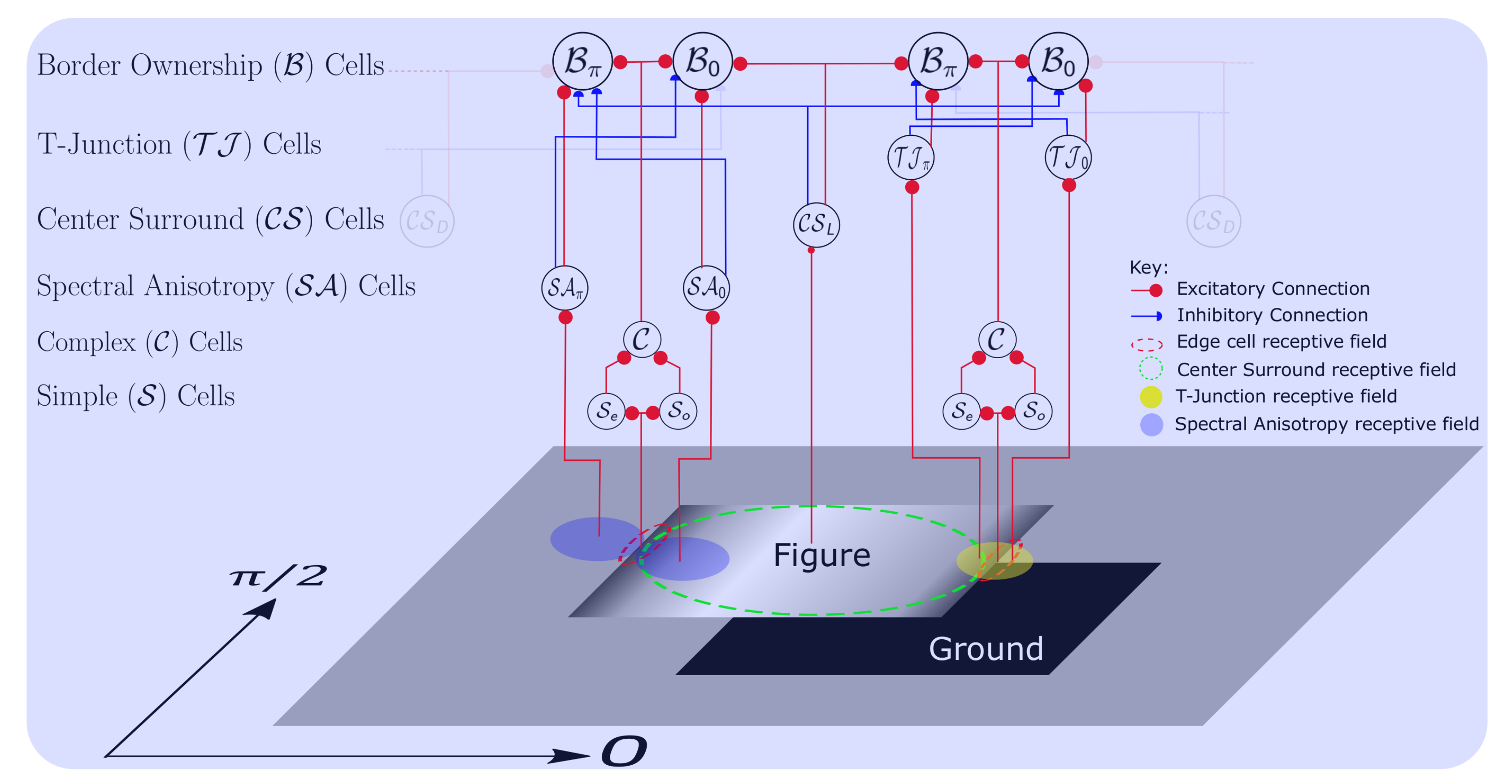
The model consists of three independent features channels, Color, Intensity and Orientation. The features are computed at multiple scales to achieve scale invariance. Orientation selective V1 Simple and Complex cells [72] are excited by edge fragments of objects within their receptive field (Figure 1). Let us denote the contrast invariant response of a Complex cell at location by , where is the preferred orientation of the cell and is the spatial frequency. As the spatial frequency (see Table 1 for all parameters of the model) is same for all edge responsive cells in the model, except when explicitly stated otherwise (Section 4.1), the variable, is omitted for the most part. Each active Complex cell, activates a pair of BO cells, one with a BO preference direction, (a counter-clockwise rotation with respect to ) denoted as , and the other with BO preference, denoted as . When the BO response related to a specific figure-ground cue is discussed, be it local or global, a subscript is added to the right of the variable. For example, would be used to denote the BO response related to T-Junctions. Likewise, when specifying scale is necessary, it is denoted by superscript, k. For example, denotes Complex cell response for orientation at location, and scale, k. On the other hand, when there is a need to explicitly specify the feature being addressed, a subscript is added to the left of the variable. For example, represents the BO response for the Color feature channel. When a specific BO direction, feature, cue, scale or a location is not important, it is just referred to as, cells, cells, and so forth. The same applies in all such situations.
Without the influence of any local or global cues, the responses of both BO cells at a location will be equal, hence the figure direction at that location is arbitrary. The center-surround cells, denoted as cells, bring about global scene context integration by modulating the cell activity. The cells (Figure 1) extract light objects on dark background, while cells code for dark objects on light background. Without the influence of local cues, this architecture embodies the Gestalt properties of convexity, surroundedness and parallelism (global cues).
The local cues (see Section 4 for computational details of local cues) modulate cell activity additionally. Similar to cells, a pair of Spectral Anisotropy cells exist for the two opposite BO preference directions at each location, which capture local texture and shading gradients (see Section 4.1 for SA computation) on the two sides of the border. Let us denote by the cell capturing Spectral Anisotropy for BO direction, likewise for the opposite BO direction. The T-Junction cells (see Section 4.2 for computational details) also come in pairs, for the two opposite BO directions. Similar to cells, hold the T-Junction cue information for the two antagonistic BO directions, . Both these type of cells excite cells of the same BO direction and inhibit the opposite BO direction cells. For example, excites and inhibits .
The influence of cells, cells and cells on cells is controlled by a set of weights (not shown in Figure 1). Local cues are active in the Orientation channel only. The interplay of all these cues leads to the emergence of figure-ground relations strongly biased for one of the two BO directions at each location. The network architecture depicted in Figure 1 is the same computational construct that is applied at every scale, for every feature and orientation. The successive stages of model computation are explained in the following subsections.
3.1. Computation of Feature Channels
Color, Intensity and Orientation are considered as three independent feature channels in the model. Each feature channel is computed at the native image resolution as explained in Section 3.1.1–Section 3.1.3. Once the feature channels are computed at the native image resolution, each feature channel, irrespective of the feature type, undergoes a feature pyramid decomposition as explained in Section 3.2 followed by BO pyramid computation as explained in Section 3.3. RGB images with with each of the R, G and B channels in range are used throughout. The differences arising due to having different number of feature sub-channels (we have one intensity channel, 4 color sub-channels and 8 orientation channels) are normalized using the normalization step (see normalization operator, , explained in Section 3.3).
The computation of each feature channel is described in the following sub-sections.
3.1.1. Intensity Channel
The input image consists of Red (r), Blue (b) and Green (g) color channels. The intensity channel, I is computed as average of the three channels, . As with all other feature channels, a multi-resolution image pyramid is constructed from the intensity channel (Section 3.2). The multi-resolution analysis allows incorporation of scale invariance into the model.
3.1.2. Color Opponency Channels
The color channels are first normalized by dividing each r, g or b value by I. From the normalized r, g, b channels, four color channels, Red (), Green (), Blue () and Yellow () are computed as,
In Equation (4), the symbol,| |denotes absolute value.
The four opponent color channels, , , and are computed as,
3.1.3. Orientation Channel
The Orientation channel is computed using the canonical model of visual cortex [72], where quadrature phase, orientation selective, Gabor kernels are used to model the V1 simple cells. The responses of Simple cells are non-linearly combined to obtain the contrast invariant, orientation selective response of the Complex cell. Mathematically, the receptive fields of even and odd symmetric Simple cells can be modeled as the cosine and sine components of a complex Gabor function—a sinusoidal carrier multiplied by a Gaussian envelope. The RF of a Simple Even cell, is given by,
where and are the rotated coordinates, is the standard deviation of the Gaussian envelope, is the spatial aspect ratio (controlling how elongated or circular the filter profile is), is the spatial frequency of the cell and is the preferred orientation of the simple cell. Similarly, the receptive field of a Simple Odd cell is defined as,
Simple even and odd cells responses, respectively denoted and are computed by correlating the intensity image, with the respective RF profiles. The Complex cell response, is calculated as,
Eight orientations in the range, , at intervals of are used.
3.2. Multiscale Pyramid Decomposition
Let us denote a feature map, be it Orientation (), Color (, , etc.) or Intensity feature map, at image resolution by a common variable, . The next scale feature map, is computed by downsampling . The downsampling factor can be either (half-octave) or 2 (full octave). Bi-linear interpolation is used to compute values in the down-sampled feature map, , which is the same interpolation scheme used in all cases of up/down sampling. Similarly, any feature map of a lower scale, k is computed by downsampling the higher scale feature map, by the appropriate downsampling factor. As the numerical value of k increases, the resolution of the map at that level in the pyramid decreases. The feature pyramids thus obtained are used to compute BO pyramids explained the next section.
In addition to the multiscale pyramids of independent feature channels, multiscale local cue pyramids for SA and T-Junctions are computed as well. To denote the local cue map at a specific scale, as with feature pyramids, the scale parameter k is used. For example, denotes the Spectral Anisotropy feature map for border ownership direction at scale, k. Similarly T-Junction pyramids at different scales for BO directions are denoted by . The local cue pyramids are computed by successively downsampling the local cue maps at native resolution, and (see Section 4 for their computation details).
3.3. Border Ownership Pyramid Computation
The operations performed on any of the features ( or I) or the sub-type of features like is the same. BO responses are computed by modulating by the activity of center-surround feature differences on either sides of the border. Each feature map, , is correlated with the center-surround filters to get center-surround () difference feature pyramids. Two types of center-surround filters, (ON-center) and are defined as,
where are the standard deviations of the outer and inner Gaussian kernels respectively.
The center-surround dark pyramid, is obtained by correlating the feature maps, with the filter followed by half-wave rectification,
which detects weak/dark features surrounded by strong/light ones. In Equation (14), the symbol, * denotes 2D correlation [73]. Two-dimensional correlation between a kernel, and an image, is defined as, , where M and N are dimensions of the image. Similarly, to detect strong features surrounded by weak background, a pyramid is computed as,
The pyramid computation is performed this way for all feature channels except for the Orientation channel. For the Orientation feature channel, feature contrasts are not typically symmetric as in the case of other features, but oriented at a specific angle. Hence, the and filter kernels in Equations (14) and (15) are replaced by even symmetric Gabor filters, (ON-center) and (OFF-center) of opposite polarity, respectively. But, in this case, different set of parameter values are used. Instead of , and used in Section 3.1.3, here , and are used respectively. The parameter values are modified in this case such that the width of the center lobe of the even Gabor filters (ON and OFF-center) matches the zero crossing diameter of the and filter kernels in Equations (14) and (15). As a result, the ON-center Gabor kernel detects bright oriented edges in a dark background, instead of symmetric feature discontinuities detected by . Similarly, the OFF-center Gabor filter detects activity of dark edges on bright backgrounds.
An important step in BO computation is normalization of the center-surround feature pyramids, and . Let be used to denote the normalization operation, which is same as the normalization used in Reference [74], but done after rescaling and pyramids to have the same range, . Similarly the local cue pyramids, and are also normalized using the same method and in the same range, . In the same way, pyramids are also normalized. This normalization step enables comparison of different features and local cues on the same scale, hence the combination of feature and local cue pyramids.
Since, BO is computed on the normalized light and dark CS pyramids, and separately and combined at a later stage, let us denote, the corresponding BO pyramids by and respectively. The BO pyramid computation for and which have a BO preference direction of is explained. Computation of and is analogous.
Let denote the kernel responsible for mapping the object activity from normalized and pyramids to the object edges, which is implemented with von Mises distribution. von Mises distribution is a normal distribution on a circle [75]. The un-normalized von Mises distribution, is defined as [63],
where pixels is the radius of the circle on which the von Mises distribution is defined, is the angle at which the normal distribution is concentrated [75] on the circle (also called mean direction), and is the modified Bessel function of the first kind. The distribution is then normalized as,
is computed analogously.
The BO pyramid, for light objects on dark background capturing the BO activity for direction is computed as,
Similarly, the BO pyramid for direction for a dark object on light background is obtained by correlating normalized maps with and summing the responses for all scales greater than the scale, k at which BO map is being computed as,
where is the synaptic weight for the inhibitory signal from the feature map of opposite contrast polarity. The symbol, ⨁ is used to denote pixel-wise addition of responses from all scales greater than k, by first up-sampling the response to the scale at which is being computed. The other two pyramids, and for the opposite BO direction are computed analogously.
With the BO pyramids related to dark and light pyramids already computed, we can turn our attention to the computation of the local cue related BO pyramids. The local cue pyramids at different scales, and are constructed, as explained in Section 4.1 and Section 4.2, by successively down-sampling the local cue maps computed at native image resolution. Both local cues excite cells of the same BO direction and inhibit the opposite BO direction cells.
The BO pyramid for BO direction related to the local cue, SA denoted as, is computed as,
where we can see the SA cell () having same BO preference as the BO cell, has an excitatory effect on the BO cell, but has an inhibitory effect. The synaptic weight, remains unchanged as in Equations (18) and (19). The BO pyramid, related to SA, for opposite BO direction is computed in the same way.
The BO pyramid related to T-Junctions for the BO direction, is computed as,
The corresponding T-Junction pyramid for the opposite BO direction, , denoted as is computed analogously.
The combined BO pyramid for direction, is computed by summing global and local cue specific BO pyramids as,
where , and are weights such that , that control the contribution of , and cues to the BO response at that location respectively. By setting the weights to 0 or 1, we can study the effect of individual cue on BO response. It should be noted that the local cues are active only for the Orientation channel, so for the other channels, and will be set to zero, by default. In the absence of local cues, combination of light and dark BO pyramids (first term in Equation (22)) results in contrast polarity invariant BO response. The corresponding BO pyramid for opposite BO preference, is computed as in Equation (22) by summing the light, dark and local cue BO pyramids of opposite BO preference.
Since the BO responses, , are computed for each orientation, there will be multiple BO responses active at a given pixel location. But the boundary between figure and ground can only belong to the figure side, that is, there can only be one winning BO response for a given location. So, the winning BO response, denoted as is computed as,
where is the orientation for which absolute difference between antagonistic pair of BO responses is maximum over all orientations. This gives the edge orientation at that location. So, the winning BO pyramid, has non-zero response at a location only if the difference between the corresponding pair of BO responses for is non-negative. The winning BO pyramid, for the opposite direction is computed analogously.
Upto this point, the computation for all feature channels is identical. Now, if we denote the feature specific winning BO pyramid for direction for the Color channel by , Intensity feature channel by and Orientation feature channel by , then the final BO map, for BO direction is computed by linearly combining the up-sampled feature specific BO maps across scales as,
where ⨁ represents pixel-wise addition of feature specific BO responses across scales after up-sampling each map to native resolution of the image. Similarly, is computed for BO direction. As we can see in Equation (24), the contribution of every feature channel to the final BO map is the same, that is, feature combination is equally weighted. Ten spatial scales () are used. All parameters of the model are summarized in Table 1. In the end, we get 16 BO maps at image resolution, 8 each for and BO directions respectively.
4. Adding Local Cues
Both local cues, SA and T-Junctions are computed at the native resolution of the image, but they influence BO cells of all scales as described in Equations (20) and (21). In other words, the cues are computed once based on the analysis local image neighborhood, but their effect is not local (Should the effect of local cues also be local? See Section 7 for related discussion).
4.1. Computation of Spectral Anisotropy
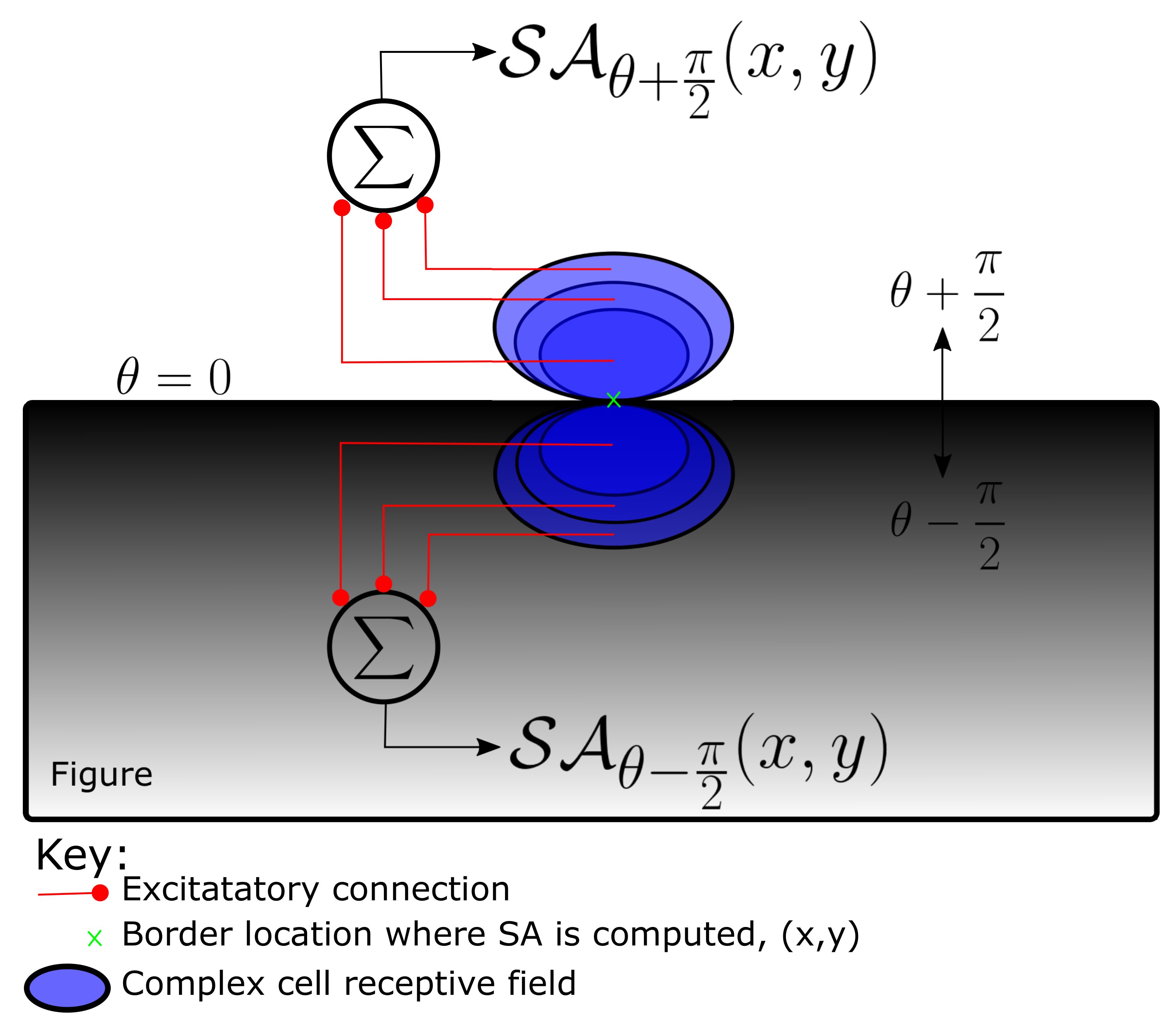
Spectral Anisotropy, a local cue for FGO, that captures intensity and texture gradients very close to object boundaries, is computed by pooling Complex cell responses of various spatial frequencies from small image regions on either sides of the boundary (Figure 2). This computation is neurally/biologically plausible.
SA at any location, in the image, for a specific orientation, and for the BO direction, is computed for one side of the border (side determined by the BO direction, ) as,
where . The Complex cell response, , is computed as explained in Section 3.1.3, but with a different set of parameters, , , instead of , and respectively. The values of , , and other relevant parameters are listed in Table 2. Filter size is equal to and r is the perpendicular distance between the point, at which SA is being computed and the center of the Gabor filters. The centers of even and odd symmetric Gabor filters, hence the Complex cell are all located at , from where the complex cell responses are pooled to compute SA. The term, determines the number of lobes in the Gabor filters. It is 2 or 4 for even symmetric Simple cells and 3 or 5 for odd symmetric Simple cells. The location from which Complex cell responses are pooled, is computed as,
Similarly, SA at the same location, , but for the opposite side of border at the same orientation, is computed as,
where,
So, for every location there will be two SA cells capturing the spatial intensity and texture gradients on the two sides abutting the border. It has to be noted that the major axis orientation of the Gabor filters is the same as the local border orientation, . This is because we want to capture the variation of spectral power in a direction orthogonal to the object boundary, which is captured by the Complex cells with their orientation parallel to the object boundary. This biologically plausible computation of SA with Complex cells responses captures the anisotropic distribution of high frequency spectral power on figure side discussed in Reference [18]. The SA maps thus obtained are decomposed into multiscale pyramids, , where superscript, k denotes scale, by successive downsampling, which are used to compute the cue specific BO pyramids as explained in Section 3.3, Equation (20).
4.2. Detecting of T-Junctions
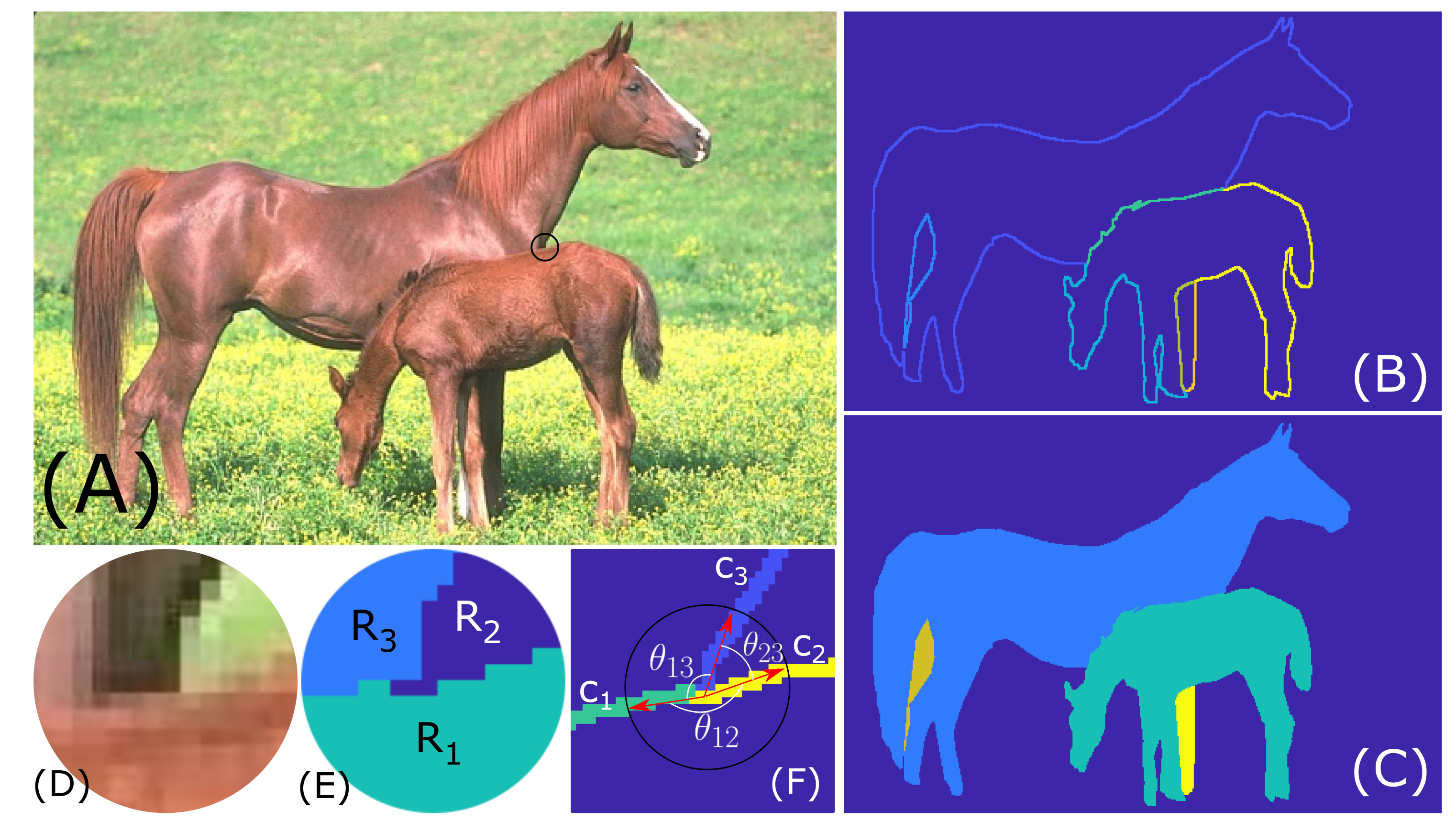
The object edges and the regions bound by those edges called “segments” are obtained using the gPb+ucm+OWT image segmentation algorithm [76], referred to as the gPb algorithm in other parts of this work. Image segmentation, partitioning of an image into disjoint regions, is considered as a pre-processing step occurring prior to FGO. The edges obtained using the gPb algorithm are represented as a Contour Map as shown in Figure 3B. The corresponding Segmentation Map is shown in Figure 3C. The Contour Map has uniquely numbered pieces of contours that appear to meet at a junction location. The Segmentation Map contains uniquely numbered disjoint regions bound by the contours. The Contour Map and Segmentation Maps are just a convenient way of representing the edge information. Only the locations at which exactly 3 distinct contours meet in the Contour Map (Figure 3B) and correspondingly the locations at which exactly 3 distinct segments meet in the Segmentation Map (Figure 3C) are considered for T-Junction determination. Such locations can be easily determined from the Segmentation and Contour maps.
As shown in Figure 3E,F, at each junction location we have three regions, , and and contours, , and meeting. At each such junction, a circular mask of pixels is applied and the corresponding small patches of the segmentation map and contour map are used for further analysis. The contours forming the “hat” of the T-Junction (foreground) and the corresponding figure direction are determined in two different ways: (1) based on the area of regions meeting at junction location within the small circular disk around junction; (2) based on the angle between contours meeting at the junction location. Finally, only those junctions locations for which figure direction, as determined based on both methods, is matching are introduced into the FGO model as T-Junction local cues. Matching based on two different methods improves the overall accuracy in correctly identifying the “hat” (foreground) and “stem” (background) of T-Junctions, in effect the correct figure direction.
The local neighborhood of T-Junction influence is set to be a circular region of radius 15 pixels. All the border pixels near the junction location within a radius of 15 pixels that belong to the “hat” of the T-Junction are set to +1 for the appropriate BO direction. Remember that for each orientation, we will have two T-Junction maps, one for the BO preference direction, denoted as and the other for the opposite BO preference, denoted as . A pixel in is set to +1 if the direction of figure, as determined by both methods (Section 4.2.1 and Section 4.2.2) is , that is, “stem” of the T-Junction is in the direction. Similarly, computed. The T-Junction maps thus obtained are decomposed into multiscale pyramids, , where superscript, k denotes scale, by successive downsampling, which are used to compute the cue specific BO pyramids as explained in Section 3.3, Equation (21).
4.2.1. Area Based T-Junction Determination
Let , and be the three regions at a junction location (Figure 3E). After extracting the circular region around the junction by applying a circular mask of radius, 6 pixels, the number of pixels belonging to each of the regions, is counted. The region, having the largest pixel count is determined as the figure region. In Figure 3E, is the region with largest pixel count, hence determined as the foreground. The contours abutting the figure region, as determined by pixel count, which are and (Figure 3F), form the “hat” of the T-Junction. Contour forms the “stem” of the T-Junction, which belongs to the background.
The local orientation at each contour location is known. Vectors of length 1–3 pixels, normal to the local orientation are drawn at each “hat” contour location within the pixel neighborhood. If the normal vector intersects the figure region, , as determined based on region area, the edge/contour location is given a value of +1 in the T-Junction map for the appropriate BO direction, which can be or . This is done for every pixel in the edge/contour map within a neighborhood of 15 pixel radius around the T-Junction location for those contours ( and ) that form the “hat” of the T-Junction. For example, in Figure 3E,F, if the local orientation of and is roughly 0, then the end point of normal vector in the direction intersects with the figure region, , as determined based on the segment area. So, the T-Junction map for BO preference direction is set to +1 within the circular neighborhood of pixels. The T-Junction map for BO direction will be zero.
4.2.2. Angle Based T-Junction Determination
In this method, as in Section 4.2.1, a small circular patch of radius, 7 pixels is extracted from the contour map around T-junction location. Pixels belonging to each contour, meeting at the junction are labeled with a distinct number, so for each contour, the first 7 pixels are tracked starting from the junction location. Since the starting point for each contour, is the same, the total angle at junction location is 360. For each contour, a vector (red arrows in Figure 3F) is defined from the junction location to the last tracked point on the contour. Then, the angle between the vectors corresponding to contours is computed. The contours between which angle is the largest form the “hat” of the T-junction. For example, in Figure 3F, is the angle between and , which is also the largest of the three angles, , and . So, in the angle based T-junction computation also, and are determined to form the “hat” of the T-junction. The figure direction at every pixel of the “hat” contours is determined as in Section 4.2.1.
Among all the potential T-Junctions determined using the angle based method, potential Y-Junctions and Arrow junctions are discarded based on the angle formed by the contours at junction location. If the largest angle is greater than 180, such junctions are discarded. Since the largest angle greater than 180 is typically seen in the case of Arrow-junctions, those are not included in the computation. Arrow junctions appear in a scene when the corner of a 3D structure is seen from outside. In the same way, if each angle at a junction location is within , such junctions are discarded as those are most likely Y-Junctions. Y-Junctions appear in a scene when a 3D corner is viewed from inside the object, for example, corner of a room viewed from inside the room. Rest of the T-Junctions are included. Angle based filtering of potential Arrow or Y-Junctions was not considered in previous methods [39,41].
T-Junctions and their figure directions are determined using both Segment Area based and Contour Angle based methods and the T-Junctions are incorporated into the model only in those cases, where both methods give matching figure direction, which makes T-Junction determination more accurate.
Accurately determining the figure side of a T-junction from a small neighborhood of 6–7 pixel radius is quite challenging because, within that small neighborhood we generally do not have any information indicative of figure-ground relations, other than contour angle and segment area. Even though key point detection is a well studied area, hence locating a T-Junction is not problematic, deciding which of the three regions is the foreground based on information from a small neighborhood is extremely challenging. So, when locally determining figure side of a T-junction, segment area and contour angle were found to be the most exploitable properties.
5. Data and Methods
The figure-ground dataset, a subset of BSDS 300 dataset, consists of 200 images of size pixels, where each image has two ground truth figure-ground labels [32] and corresponding boundary maps. For each image, the two sets of figure-ground labels labels are annotated by users other than those who outlined the boundary maps. The figure-ground boundary consists of figure side of the boundary marked by +1 and the ground side boundary by −1.
The figure-ground classification accuracy (FGCA) for an image that is reported is the percentage of the total number of boundary pixels in the ground truth figure-ground label map for which a correct figure-ground classification decision is made by the model described in Section 3. Even though the model computes BO response at every location where cells are active, the BO responses are compared only at those locations for which ground truth figure-ground labels exist.
Whenever the two ground truth label maps differ for the same image, average of the FGCA for both ground truth label maps is reported. Since different figure-ground labelers interpret figure and ground sides differently depending on the context, such differences arise, as a result, the self-consistency between figure-ground labelings between the two sets of ground truth annotations is 88%, which is the maximum achievable FGCA for the dataset. At each pixel, the direction of figure, as determined by the model can be correct or wrong. So, the average FGCA for the entire dataset, at chance is 50%, assuming figure-ground relations at neighboring pixels are independent. This assumption is consistent with previously reported results [32], where same assumption was made. The complete details of the figure-ground dataset can be found in References [6,32,77].
The entire BSDS figure-ground dataset consisting of 200 images is randomly split into training set of 100 images and test set of 100 images. Parameters of the model are tuned for the training dataset and the optimal values of parameters found for the training set are used to evaluate the FGCA of the test set of images. The average FGCA that is reported for the entire test set is the average of FGCAs of all 100 images in the test set.
6. Results
To remind the readers, the model with only global cues of convexity, surroundedness and parallelism, without any local cues is referred to as the Reference model. As explained in Section 3, local cues, SA and T-Junctions are added to the Orientation feature channel of the reference model. As previously described in Section 3.3, by setting and in Equation (22), the model with local cues can be reduced to the reference model. Similarly, by switching the weights for each local cue to zero, the effect of the other local cue on FGO can be studied. As explained in Section 3.3, the winning BO pyramids are up-sampled to image resolution and summed across scales and feature channels (Equation (24)) for each BO direction to get the response magnitude for that BO direction. The BO information derived this way is compared against the ground-truth from BSDS figure-ground dataset.
First, the performance of the reference model, which is devoid of both local cues, is quantified in terms of FGCA. With and , the overall FGCA for 100 test images was 58.44% (standard deviation = 0.1146). With only global cues, the 58.44% FGCA that was achieved is 16.88% above chance level (50%). Hence, it can be concluded that the global Gestalt properties of convexity, surroundedness and parallelism, which the reference model embodies, are important properties that are useful in FGO. The parameters used in the reference model computation are listed in Table 1. Unless stated otherwise explicitly, those parameters in Table 1 remain unchanged for the remaining set of results that are going to be discussed. Only the parameters specifically related to the addition of local cues are separately tuned and will be explicitly reported.
Next, the effect of adding each local cue individually (Section 6.1 and Section 6.2) and then the effect of both local cues together (Section 6.3) are studied.
6.1. Effect of Adding Spectral Anisotropy
As explained in Section 4.1, Spectral Anisotropy was computed at the native resolution of the image by pooling Complex cell responses at many scales for each orientation. For each orientation, , two SA maps, and are created for respective antagonistic BO directions with respect to . The SA maps are then decomposed into multiscale pyramids by successively downsampling. The SA pyramids are then incorporated into the model as explained in Equations (20) and (22). In this case, parameters and are tuned for the training dataset and is set to 0.
The parameter tuning procedure used here is the same for other cases as well. Multi-resolution grid search is used for parameter tuning with the condition that the sum of tuned parameters should be 1. In this case, the condition was . Refinement of the resolution of the grid is stopped when the variation in FGCA upto second decimal point is zero, that is, only small changes are seen from third digit onward, after the decimal point.
The optimal parameters were found to be, and for the training dataset. With these optimal parameter values, the FGCA for the test set was 62.69% (std. dev = 0.1204), which is a 7.3% improvement in the model’s performance after adding the local cue, Spectral Anisotropy, compared to the reference model’s FGCA of 58.44%. To verify if the improvement in FGCA that we see is statistically significant, an unpaired sample, right tailed t-test (Table 3) is performed, where the null hypothesis was that the means of FGCAs of the reference model and the model with SA are equal. The alternate hypothesis was that the mean FGCA of the model with SA is higher than that of the reference model. The significance level, was chosen. For other results (Section 6.2 and Section 6.3) as well, same type of test is done, where the reference model’s FGCA is compared with that of modified model’s FGCA having different local cues. Hereafter, let us refer to them as statistical tests.
Statistical tests show that the mean FGCA of the model with SA is significantly higher than that of the reference model (). This demonstrates SA is a useful cue and can be successfully incorporated into the reference model, adding which results in statistically significant improvement in the model’s performance. This, and all other results are summarized in Table 3 for the test dataset.
6.2. Effect of Adding T-Junctions
As described in Section 4.2, T-Junctions are computed at image resolution using the segmentation map and edge map obtained using the gPb [76] algorithm. Each of the T-Junction maps for the 16 different BO directions is successively downsampled to create multiscale T-Junction pyramids. The T-Junction pyramids are incorporated into the model as explained in Equations (21) and (22) and by setting . The other two parameters, and are tuned on the training dataset. With optimal parameter values, and (and ), the FGCA for the test set was found to be 59.48% (std. dev. = 0.1127). Compared to the reference model’s FGCA of 58.44%, we see that adding T-Junctions improves the model’s performance in terms of FGCA by 1.78%. Based on the statistical tests (Table 3), we find that the improvement in FGCA that we see is indeed statistically significant.
6.3. Effect of Adding Both Spectral Anisotropy and T-Junctions
SA is computed as explained in Section 4.1, T-Junctions are computed as explained in Section 4.2, where T-Junctions are derived from automatically extracted edges using the gPb algorithm. Both cues are added to the Reference model according to Equation (22). The parameters , and are tuned simultaneously on the training dataset using multiresolution grid search as before, with the constraint, . The optimal values of the parameters were found to be, , and . All other parameters remained unchanged as shown in Table 1. The FGCA of the combined model with both local cues, Spectral Anisotropy and T-Junctions was 63.57% (std. dev = 0.1179) for the test dataset, which is higher that the FGCAs that were obtained for the individual cues when they were added separately. An improvement in FGCA of 8.78% is observed compared to that of the reference model with no local cues. As before, an unpaired sample, right tailed t-test comparing the reference model’s figure-ground decisions and the combined model’s figure-ground decisions with both SA and T-Junctions showed statistically significant improvement (Table 3).
In addition to comparing the performance of the model with both local cues with the Reference model, the performance of the model with both local cues (Ref model + SA + T-Junctions) is compared to the model with only one (Ref model + SA) local cue. Unpaired sample right-tailed t-tests were used again with a significance level of 0.05. In this case the the null hypothesis is that adding T-Junctions to the Reference Model with SA does not lead to statistically significant improvement in FGCA. The alternate hypothesis is that adding T-Junctions leads to statistically significant improvement in FGCA when compared to the FGCA of Reference (global cues only) + SA model. Tests show adding T-Junctions to the Reference + SA model leads to a statistically significant improvement (p = ).
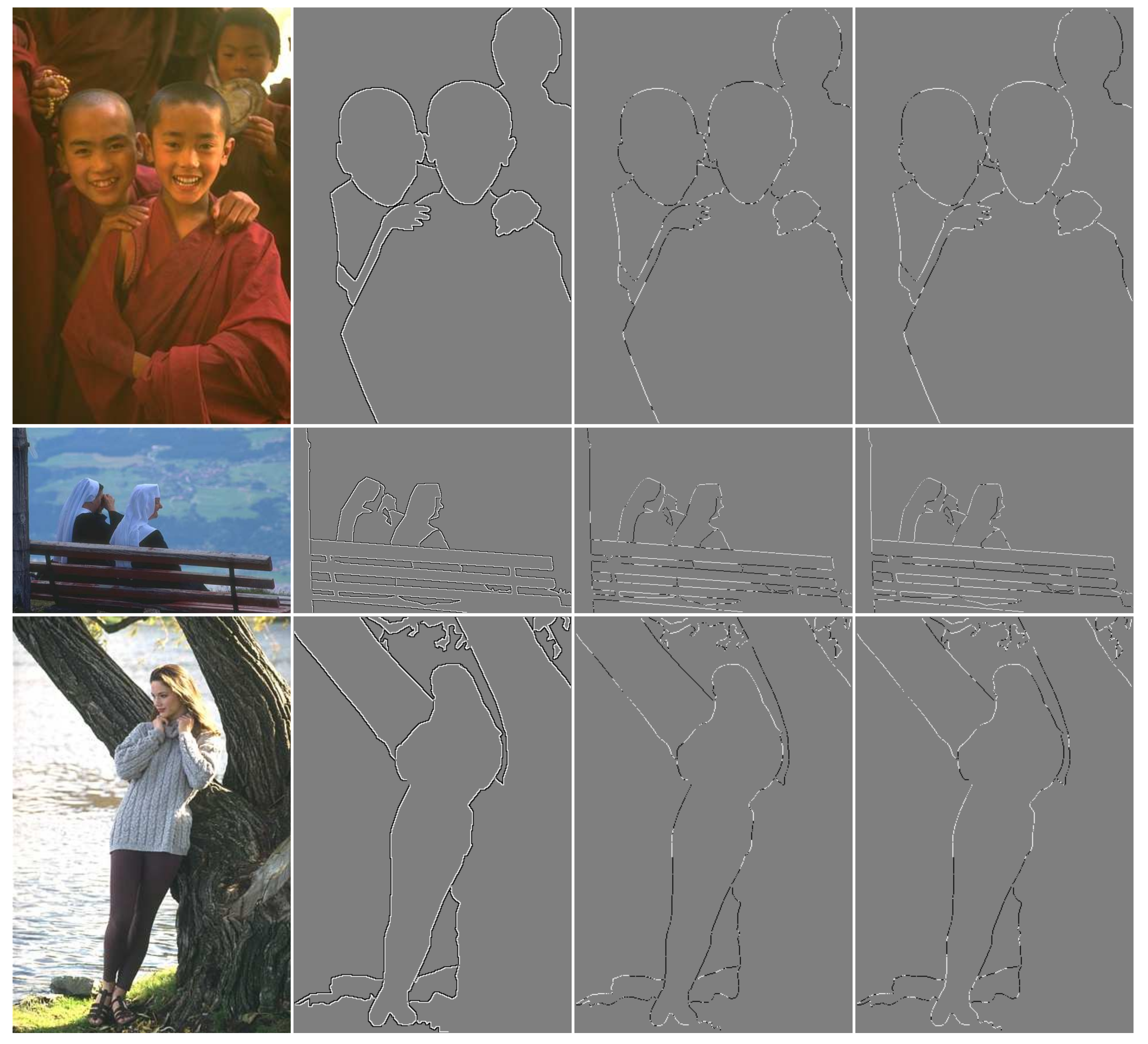
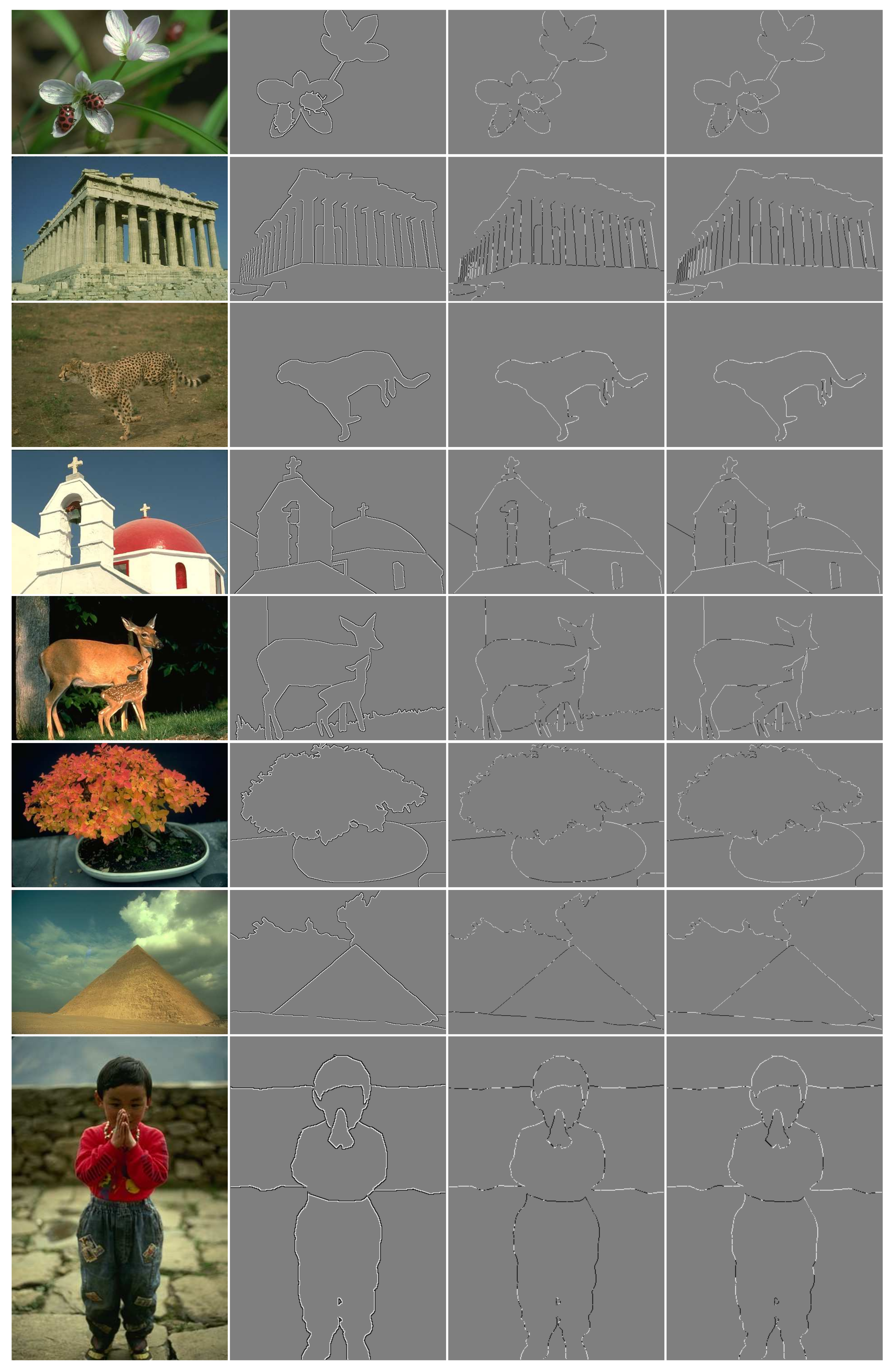
In summary, it is shown that both SA and T-Junctions are useful local cues of FGO, which produce statistically significant improvement in FGCA when added alone. When both cues are simultaneously present, they lead to even higher improvement in FGCA of the model indicating the cues are mutually facilitatory. An improvement of with only a few local and global cues at a minimal computational cost (see Appendix A for computational cost analysis) is truly impressive. Figure 4 and Figure 5 show FGO results for some example images from the test dataset when both SA and T-Junctions are added. In Figure 4 and Figure 5, it is important to notice that the groundtruth (Column 2) is 2 pixels wide, whereas the results in Columns 3–4 are only one pixel wide. In Column 2, a white pixel belongs to the figure side, whereas a black belongs to the background side. But, notice that in Columns 3–4, a white pixel indicates a correct decision was made by the model at that boundary location, whereas a black pixel (both white and black pixels are on gray background) indicates an incorrect decision was made by the model.
Next, the performance of the proposed model is compared with state of the art methods for which all steps are fully automated (see Table 4). Here, the FGCA of the model with both local cues is compared with other methods that are not neurally inspired, instead are learning based and trained on thousands of images. The proposed model performs better than that of Maire [46] even when it has only a few local and global FGO cues and not specifically tuned for best performance. The performance of the proposed model is competitive with the state of the art models given the constraints discussed above, but leaves room for improvement. The performance of the model can be substantially improved by making several simple modifications and adding more local and global cues as discussed in Section 9.
7. Discussion
We see ≈9% improvement in FGCA of the combined model with both local cues. This improvement, from only two local cues added to one of the three feature channels is truly impressive. Moreover, the three feature channels (Color, Intensity and Orientation) were weighted equally. Better results can be achieved if the weights for individual feature channels are tuned. But, since the objective here was to study how to integrate local and global cues and measure the relative importance of local cues in FGO, feature specific weight tuning was not done, but planned to be done in the future (See Section 9 for future work). Moreover, it is important to note that FGCA of the model with both local cues is always higher than the FGCAs of models with individual local cues. This suggests the local cues are mutually facilitatory, which is further validated by the fact that a statistically significant improvement is seen in FGCA when T-Junctions are added as an additional cue to the Reference model having SA as one of the local cues.
A few novel methods are introduced in the this work. First, demonstrating that Spectral Anisotropy can be computed with Simple and Complex cells found in area V1 is a novel contribution. The significance of this computation is that it demonstrates SA can be computed in low level visual areas, even in the striate cortex and it does not require specialized cells to detect these shading/texture gradients. Only a specific arrangement of Complex cells of various spatial frequencies on each side of the border is sufficient. These cues, first mathematically shown to be useful by Huggins et al. [8], were psychophysically validated by Palmer and Ghose [9]. It was shown that these patterns are abundantly found in natural images [10] and can be efficiently computed using 1D FFTs [18]. Now, it is shown that these cues can be computed in a biologically plausible manner, using Complex cells found commonly in striate cortex.
Next, in the detection of T-Junctions, Y-Junctions and Arrow junctions are filtered out using the angle property of these junction types. Since Y-Junctions and Arrow junctions are not occlusion cues, ideally those should not be considered as T-Junctions, hence a method to remove such junctions was devised. To the best of our knowledge, previous methods [39,40,41] that use T-Junctions as FGO cues have not looked closely at this issue, which can be considered novel in this work. Also, the local figure-ground relations at a T-Junction local are explicitly computed based on local information, which is new. And, the way the local cue computation is organized such that the same computational routine can be used for incorporation of both cues into the model is noteworthy. With this, the implementation is made more efficient, allowing easy parallelization using Graphics Processing Units (GPU) and other hardware. Moreover, the combination of features and local cues is done at a late stage (Equation (22)), which allows independent and parallel computation of features and local cues, which again makes the model computationally more efficient, allowing parallelization.
Even though we see ≈2% FGCA improvement when T-junctions are added, it is a relatively small, but statistically significant, improvement compared to that adding SA. Since T-Junctions are generally regarded as strong cues of occlusion, this small, statistically significant improvement may seem counter-intuitive. But it is important to note that T-Junctions are extremely sparse, can be computed only at a few locations where exactly 3 different regions partially occlude each other, whereas SA can be computed at every border location of an object. Given the sparsity of T-junctions, they can still be considered stronger FGO cues compared to SA. The presence of “inverted” T-Junctions [39,40,41], could also be the reason for diminished effect of T-Junctions. From a computational cost perspective (Appendix A), even though the cost is , given their sparsity (typically 3–10 T-Junctions per image), adding them as a local cue is justified.
Even though it is commonly assumed that T-Junctions are unambiguous cues of occlusion, no systematic, data-driven analysis of the utility of T-Junctions as a classic Gestalt cue was available until now. Moreover, there are few instances where researchers argue from the opposite perspective. Tse and Albert [78] argue that high level surface and volume analysis takes place first, and only after such an analysis, a T-Junction is interpreted to be an occlusion cue. As a result, we may not consciously notice the prevalence of “inverted” T-Junctions.
The traditional view that T-Junctions are unambiguous cues of occlusion has also been challenged by psychophysics experiments of McDermott [79], where they find that making occlusion decisions from a small aperture, typically a few pixels wide, in real images is hard for humans. Some studies also suggest junctions in general, hence T-Junctions, can be cues for image segmentation, but not for occlusion reasoning [80]. These previous works and the results from this model do not support the generally held view that T-Junctions are the most unambiguous occlusion cues. But, these cues are useful and produce statistically significant improvement in FGCA. This is an important contribution of this work.
While comparing the performance of the proposed model with existing methods, as noted in Section 6.3, we need to keep in mind some important differences. First, the model we presented is not trained on image features, hence generalization to any other dataset does not require additional training. Second, the proposed model is neurally inspired, built to provide a general framework for incorporating and studying local and global Gestalt cues, not specifically optimized for best accuracy. Moreover, only a handful of cues are used, yet this model performs better than some existing models (Maire [46] in Table 4). While Maire [46] uses 64 different shapemes, descriptors of local shape derived from object edges, Ren et al. [32] incorporates empirical frequencies of 4 different junction types derived from training data, in addition to shapemes in a Conditional Random Field based model. Also, Ren et al. [32] compare figure-ground relations with the ground-truth only at a partial set of locations where their edge detection algorithm finds a matching edge with the ground-truth. It is not clear what percentage of edges match with the ground-truth. Palou and Salembier [39] use 8 color based cues, in addition to T-Junctions and local contour convexity in their model. The other two ([33,34]) models use a much larger number of cues to achieve FGO. Moreover, the state-of-the-art models that are compared with are neither strictly Gestalt cue based nor neurally motivated. To the best of our knowledge, there are no comparable neurally inspired, feed-forward, fully automated models that are tested on the BSDS figure-ground dataset. The model proposed by Sakai et al. [68] is tested on BSDS FG database, but it requires human drawn contours.
The method that is used in this work to report FGCA can be very different from the methods of other models listed in Table 4. Here, the average FGCA of all pixels for all 100 test images is reported, which can be considerably lower than computing the FGCA image by image and then averaging the FGCA of all images. It is not clear from other methods in Table 4, how the FGCA numbers were reported. Moreover, the exact split of the dataset into train and test set also has an effect. For some splits, the FGCA can be higher. The methods reported in Table 4 may not have used the same test/train split as it is not reported in previous methods. So, instead of comparing with existing methods in terms of absolute FGCA, a more appropriate way to look at results from this work would be from the perspective of relative improvement after adding each cue. From this perspective, we do see statistically significant improvement with the addition of each local cue. Moreover, the motivation of this study is to quantify the utility of local and global cues and build a general framework to incorporate and study the effect of multiple local and global cues.
Should the influence of local cues should be strictly local or global? In the proposed model, even though the local cues, SA and T-Junctions, are computed based on the analysis of a strictly local neighborhood around the object boundary, they modulate the activity of cells at all scales, that is, their influence is global in nature. But, are the influences of local cues also local? To answer this question, local cues are added only at the top 2 layers of the model, tuned the optimal parameters, , and accordingly and recomputed FGCA. We find that with local cue influence at only the top two layers, the FGCA we obtain is lower than having them at all scales (See Appendix B for details). This confirms that the influence of local cues should not be local, even though their computation should be strictly local to reduce the computational cost, which is the case in this proposed model.
An important observation about the model is the distribution of weights (, and ) in different settings. As we can observe, the weight assigned to each cue varies inversely with the sparsity of the cue. Hence, we use markedly higher values for when it is combined with the Reference model. This is because the receptive field (RF) corresponding to a cell that detects a local cue is much smaller compared to the RF of cells that integrate global cues such as convexity, surroundedness, and so forth. Physiologically, the cells responsible for local cues are typically found in areas V1/V2 (Macaca mulatta) of the visual cortex which have much smaller RFs compared to those cells that integrate global cues, which are found in higher areas of the cortex. As a result, to capture the contribution of these local cues and globalize their effect, higher weights had to be assigned.
Another important question is about the contribution of global cues vis-a-vis local cues, especially, Spectral Anisotropy, since SA can be computed a every border location. Even though, SA can be computed at every border location, anisotropic distribution of oriented high frequency spectral power is not present at every location on the border. This is because, SA arises out of surface curvature of foreground objects and all objects do not curve on themselves [21,22]. Moreover, as explained before, the RFs of local cues are much smaller compared to the size of an object. Objects can often occupy half or the entire visual field of view. This means, local cues alone cannot create the perception of an object. So, only in the context of global properties such as convexity, surroundedness and symmetry, local cues become important. Even though, from a computational modeling perspective, it may seem local cues alone are sufficient, it is perhaps, not neurally plausible. Hence, we consider the global cues to be always present and only in the context of global cues, the contribution and interaction of local cues is studied.
Finally, is important to acknowledge that FGO is a complex process mediated through an interplay of local and global cues, feedback and recurrent connections between neurons of different layers of the cortical column. In a purely feed-forward model such as the proposed model, these aspects are not accounted for. But, given a minimalistic model with only a handful of cues, the performance of the model is noteworthy.
8. Conclusions
A biologically motivated, feed-forward computational model of FGO with local and global cues was presented. Spectral Anisotropy and T-Junctions are the local cues newly introduced into the model, which only influence the Orientation channel among the three feature channels. First, it was shown that even the reference model, with only a few global cues, convexity, surroundedness and parallelism, completely devoid of any local cues performs significantly better than chance level (50%) achieving a FGCA of 58.44% on the BSDS figure-ground dataset. Each local cue, when added alone leads to statistically significant improvement in the overall FGCA, compared to the reference model devoid of local cues, indicating their usefulness as independent local cues of FGO. The model with both SA and the T-Junctions achieves an 8.77% improvement in terms of FGCA compared to that of the model without any local cues. Moreover, the FGCA of the model with both local cues is always higher than that of the models with individual local cues, indicating the mutually facilitatory nature of local cues. In conclusion, SA and T-Junctions are useful, mutually beneficiary local cues and lead to statistically significant improvement in the FGCA of the feed forward, biologically motivated FGO model, either when added alone or together.
As shown in Appendix A, the computational complexity of adding both local cues is relatively low, yielding ≈9% improvement in model’s performance. Given that the feature channel weights are un-optimized, model consists of only a few global and local cues, local cues added to only one of three feature channels and the model is not optimized for best FGCA (See Chapter Section 9 for a discussion on how FGCA of the model can be improved even with existing local cues), the performance of the model is highly impressive.
9. Future Work
In future, one can improve the FGCA of the model by tuning the inhibitory weight, for each feature and each local cue (Equations (18)–(21)) and tuning feature specific weights in Equation (24). In addition, increasing the number of scales, having cells and cells of multiple radii can all lead to better FGCA. cells cells of multiple radii would capture the convexity and surroundedness cues better. Also, the model’s figure-ground response is computed by modulating the activity of cells, which are computed using Gabor filter kernels. The response of cells may not always exactly coincide with human drawn boundaries in the ground-truth, with which the model’s response is compared to calculate FGCA. Hence, averaging the BO response in a small pixel neighborhood and then comparing that with the ground-truth FG labels could yield improved FGCA. In future, one can explore these ideas in order to improve FGCA. Moreover, color based cues [81,82], global cues such as symmetry [83] and medial axis [84] can be incorporated to improve the FGCA and make the model more robust.
In the biologically plausible SA computation Section 4.1, the Complex cell responses were used in all the computations. It would be interesting to see if similar or better FGCA can be achieved with Simple Even or Odd cells alone. In that case, the cost of computing SA would reduce by more than half. This would make the overall FGO model computation even more efficient. Also, in Section 4.1, filter size increment was in steps of 2 pixels. Having finer filter size resolutions (for example, instead of ) will be considered to improve the FGCA even more.
From a computational cost perspective, image segmentation using the gPb [76] algorithm is the most expensive step in the FGO model with local cues. In order to decrease the computational cost, more efficient image segmentation algorithms should be explored. One efficient algorithm with similar performance as gPb (F-score, Arbelaez et al. [76] = 0.70 vs. F-score, Leordeanu et al. [85] = 0.69 on BSDS 500 dataset) by Leordeanu et al. [85] is a good candidate. Replacing gPb [76] algorithm with the algorithm by Leordeanu et al. [85] for image segmentation, hence T-Junction computation, can substantially reduce the computational overload, while achieving similar performance. Other recent methods with better image segmentation performance can also be considered. Parallelization of the model using GPUs and FPGAs can also be considered in the future.
Funding
This research received no external funding.
Conflicts of Interest
The authors declare no conflict of interest.
Appendix A. Computational Complexity and Cost of Adding Local Cues
The most computationally intensive part of SA computation is the correlations involved in Equation (25), which has a computational complexity of when implemented in Fourier domain, where and are the number of rows and columns in the image.
The computationally intensive part of T-junction computation is the gPb [76] based image segmentation. We utilize this algorithm as is, hence we will not delve into exact estimation of computational complexity for this step. Once the contours and segmentation maps are obtained using gPb algorithm, the computation of each T-Junction using both methods described in Section 4.2.1 and Section 4.2.2 involves multiplying the edge maps, segmentation maps with masks of appropriate sizes, counting and tracking pixels, computing angles, and so forth, which roughly translates into a computational complexity of for both methods, where pixels for Segment Area based T-Junction computation (Section 4.2.1) and pixels for Contour Angle based T-Junction computation (Section 4.2.2). Typically 3–10 T-Junctions are found in an image. So, once edges/segmentation map is computed, since only few T-Junctions are typically present in images and the size of mask is not very large, subsequent computation is not very time consuming. With appropriate modifications, it should be possible to reduce the computational complexity of T-Junction determination even further, which is not optimized at the moment.
In terms of computational cost, we focus only on the cost/overhead of adding new local cues to the Reference model. The number of FLOPs for basic arithmetic operations (addition, subtraction, multiplication) are counted as 1 FLOP, comparison as 1 FLOP, division, square root of a number as 4 FLOPs, exponential, trigonometric functions as 8 FLOPs, and so forth. These estimates are based on Reference [86]. The computational cost measured in FLOPs for an image for different versions of the model are summarized in this section. The image size is always, pixels, the size of all images in the BSDS Figure/Ground dataset.
- Reference model computation-no local cues: 133,787,537,703 FLOPs
- Reference model + SA (current implementation): 170,001,489,671. As stated in Section 9, the computational cost of SA can be reduced by using a fixed size filter, reducing the number of orientations and using only Simple cell responses. Without these optimizations, the overhead is 27.068%. Having these optimization, in an ideal implementation, would dramatically reduce the computational overhead.
- Reference model + SA (ideal implementation): 143,393,171,688 FLOPs (computational overhead: 7.17%). In the ideal case, filter size would be kept constant and SA would be computed based on image pyramid. Moreover, by reducing the number of orientations to 4, instead of 8, the cost can be reduced by half to ≈3.5%. Additionally, only Simple cells can be used to reduce the computational cost even more (See Section 9).
- Reference model + T-Junctions (without edge segmentation step): 141,749,861,545 FLOPs (computational overhead: 5.95%)
Overall, with ideal implementation, the overhead of adding local cues could be ∼5–15% for gain in FGCA of %. For the model with both local cues, generating the figure-ground decision map for an image from BSDS dataset takes ∼7–10 s on a Linux workstation with Intel Core i7 CPU with 8GB RAM. However, we have not systematically measured the memory requirements and computational time.
Appendix B. Local Cues Influencing Only Top 2 Layers
Should the influence of local cues also be strictly local? Local cues, by definition, should be computed based on the analysis of a small patch of an image to determine figure-ground relations. This is what makes them computationally more efficient. But, should their influence also be local? There is no a priori reason why their influence should be strictly local. To verify whether there is higher benefit in adding them locally only at the top layer (i.e., at native image resolution only), we added them only at the top layer. For SA it resulted in a noticeable, but very small improvement. For T-Junctions, the change was barely noticeable. This could be due to extremely small size of von Mises filter kernels that we use ( pixels) in comparison with the images size ( pixels). So, we added the local cues to the top two layers. For each local cue added separately, the optimal parameters of the model were recomputed and those parameters were used to compute the FGCA. The versions of the model with local cues only at the top 2 layers did not give rise to better FGCA than what we saw earlier with the cues added at all scales. The results are summarized in Table A1.

Table A1.
Local cues only at the top 2 layers: By adding each local cue only at the top 2 layers (), we see the FGCA we obtain is much lower than having them at all levels ().
Table A1.
Local cues only at the top 2 layers: By adding each local cue only at the top 2 layers (), we see the FGCA we obtain is much lower than having them at all levels ().
| Model | K = 2 | K = 10 |
|---|---|---|
| Ref Model | - | 58.44% |
| Ref + SA | 62.42% | 62.69% |
| Ref + T-Junctions (gPb edges) | 59.12% | 59.48% |
References
- Wagemans, J.; Elder, J.H.; Kubovy, M.; Palmer, S.E.; Peterson, M.A.; Singh, M.; von der Heydt, R. A century of Gestalt psychology in visual perception: I. Perceptual grouping and figure–ground organization. Psychol. Bull. 2012, 138, 1172. [Google Scholar] [CrossRef] [PubMed] [Green Version]
- Wagemans, J.; Feldman, J.; Gepshtein, S.; Kimchi, R.; Pomerantz, J.R.; van der Helm, P.A.; van Leeuwen, C. A century of Gestalt psychology in visual perception: II. Conceptual and theoretical foundations. Psychol. Bull. 2012, 138, 1218. [Google Scholar] [CrossRef] [PubMed] [Green Version]
- Koffka, K. Principles of Gestalt Psychology; Harcourt-Brace: New York, NY, USA, 1935. [Google Scholar]
- Bahnsen, P. Eine Untersuchung uber Symmetrie und Asymmetrie bei visuellen Wahrnehmungen. Z. Fur Psychol. 1928, 108, 129–154. [Google Scholar]
- Palmer, S.E. Vision Science-Photons to Phenomenology; MIT Press: Cambridge, MA, USA, 1999. [Google Scholar]
- Fowlkes, C.; Martin, D.; Malik, J. Local figure-ground cues are valid for natural images. J. Vis. 2007, 7, 2. [Google Scholar] [CrossRef] [PubMed] [Green Version]
- Heitger, F.; Rosenthaler, L.; von ver Heydt, R.; Peterhans, E.; Kübler, O. Simulation of neural contour mechanisms: From simple to end-stopped cells. Vis. Res. 1992, 32, 963–981. [Google Scholar] [CrossRef]
- Huggins, P.; Chen, H.; Belhumeur, P.; Zucker, S. Finding folds: On the appearance and identification of occlusion. In Proceedings of the IEEE Computer Society Conference on Computer Vision and Pattern Recognition, Kauai, HI, USA, 8–14 December 2001; Volume 2, pp. 2–718. [Google Scholar]
- Palmer, S.; Ghose, T. Extremal edges: A powerful cue to depth perception and figure-ground organization. Psychol. Sci. 2008, 19, 77–84. [Google Scholar] [CrossRef]
- Ramenahalli, S.; Mihalas, S.; Niebur, E. Extremal edges: Evidence in natural images. In Proceedings of the 45th Annual Conference on Information Sciences and Systems (CISS), Baltimore, MD, USA, 23–25 March 2011; pp. 1–5. [Google Scholar]
- Zhou, H.; Friedman, H.S.; von der Heydt, R. Coding of border ownership in monkey visual cortex. J. Neurosci. 2000, 20, 6594–6611. [Google Scholar] [CrossRef] [Green Version]
- Williford, J.R.; von der Heydt, R. Figure-ground organization in visual cortex for natural scenes. eNeuro 2016, 3. [Google Scholar] [CrossRef] [Green Version]
- Craft, E.; Schutze, H.; Niebur, E.; von der Heydt, R. A neural model of figure-ground organization. J. Neurophysiol. 2007, 97, 4310–4326. [Google Scholar] [CrossRef]
- Roelfsema, P.R.; Lamme, V.A.; Spekreijse, H.; Bosch, H. Figure ground segregation in a recurrent network architecture. J. Cogn. Neurosci. 2002, 14, 525–537. [Google Scholar] [CrossRef] [Green Version]
- Zhaoping, L. Border ownership from intracortical interactions in visual area V2. Neuron 2005, 47, 143–153. [Google Scholar] [CrossRef] [PubMed] [Green Version]
- Mihalas, S.; Dong, Y.; von der Heydt, R.; Niebur, E. Mechanisms of perceptual organization provide auto-zoom and auto-localization for attention to objects. Proc. Natl. Acad. Sci. USA 2011, 108, 7583–7588. [Google Scholar] [CrossRef] [PubMed] [Green Version]
- Hu, B.; von der Heydt, R.; Niebur, E. Figure-Ground Organization in Natural Scenes: Performance of a Recurrent Neural Model Compared with Neurons of Area V2. eNeuro 2019, 6. [Google Scholar] [CrossRef] [PubMed] [Green Version]
- Ramenahalli, S.; Mihalas, S.; Niebur, E. Local spectral anisotropy is a valid cue for figure–ground organization in natural scenes. Vis. Res. 2014, 103, 116–126. [Google Scholar] [CrossRef] [Green Version]
- Ramenahalli, S.; Mihalas, S.; Niebur, E. Figure-ground classification based on spectral anisotropy of local image patches. In Proceedings of the 46th Annual IEEE Conference on Information Sciences and Systems (IEEE-CISS), Princeton, NJ, USA, 21–23 March 2012; pp. 1–5. [Google Scholar]
- Ramenahalli, S.; Mihalas, S.; Niebur, E. Spectral inhomogeneity provides information for figure-ground organization in natural images. In Proceedings of the Society for Neuroscience Annual Meeting, Washington, DC, USA, 12–16 November 2011. [Google Scholar]
- Ghose, T.; Palmer, S. Extremal edges versus other principles of figure-ground organization. J. Vis. 2010, 10, 3. [Google Scholar] [CrossRef]
- Palmer, S.; Ghose, T. Extremal edges dominate other cues to figure-ground organization. J. Vis. 2006, 6, 96. [Google Scholar] [CrossRef]
- Rubin, E. Visuell wahrgenommene Figuren. In Visual Perception: Essential Readings; Yantis, S., Ed.; Psychology Press: London, UK, 2001. [Google Scholar]
- Schirillo, J.A. The anatomical locus of T-junction processing. Vis. Res. 2009, 49, 2011–2025. [Google Scholar] [CrossRef] [Green Version]
- Heitger, F.; von der Heydt, R. A computational model of neural contour processing: Figure-ground segregation and illusory contours. In Proceedings of the 4th International Conference on Computer Vision, Berlin, Germany, 11–14 May 1993; IEEE Computer Society Press: Los Alamitos, CA, USA, 1993; pp. 32–40. [Google Scholar]
- Hansen, T.; Neumann, H. A Biologically Motivated Scheme for Robust Junction Detection. In Proceedings of the Second International Workshop on Biologically Motivated Computer Vision, Tübingen, Germany, 22–24 November 2002; pp. 16–26. [Google Scholar] [CrossRef] [Green Version]
- Rubin, E. Visuell Wahrgenommene Figuren; Glydenalske Boghandel: Kobenhaven, Denmark, 1921. [Google Scholar]
- Wertheimer, M. Untersuchungen zur Lehre von der Gestalt II. Psychol. Forsch. 1923, 4, 301–350. [Google Scholar] [CrossRef]
- Lamme, V.A. The neurophysiology of figure-ground segregation in primary visual cortex. J. Neurosci. 1995, 15, 1605–1615. [Google Scholar] [CrossRef]
- Super, H.; Lamme, V.A. Altered figure-ground perception in monkeys with an extra-striate lesion. Neuropsychologia 2007, 45, 3329–3334. [Google Scholar] [CrossRef]
- Williford, J.R.; von der Heydt, R. Early Visual Cortex Assigns Border Ownership in Natural Scenes According to Image Context. J. Vis. 2014, 14, 588. [Google Scholar] [CrossRef]
- Ren, X.; Fowlkes, C.C.; Malik, J. Figure/ground assignment in natural images. In European Conference on Computer Vision; Springer: Berlin/Heidelberg, Germany, 2006; pp. 614–627. [Google Scholar]
- Hoiem, D.; Efros, A.A.; Hebert, M. Recovering occlusion boundaries from an image. Int. J. Comput. Vis. 2011, 91, 328–346. [Google Scholar] [CrossRef]
- Teo, C.L.; Fermüller, C.; Aloimonos, Y. Fast 2D Border Ownership Assignment. In Proceedings of the IEEE Conference on Computer Vision and Pattern Recognition, Boston, MA, USA, 7–12 June 2015; pp. 5117–5125. [Google Scholar]
- Hoiem, D.; Stein, A.N.; Efros, A.A.; Hebert, M. Recovering occlusion boundaries from a single image. In Proceedings of the IEEE 11th International Conference on Computer Vision, ICCV, Rio de Janeiro, Brazil, 14–21 October 2007; pp. 1–8. [Google Scholar]
- Amer, M.R.; Raich, R.; Todorovic, S. Monocular Extraction of 2.1D Sketch. In Proceedings of the International Conference on Image Processing, ICIP 2010, Hong Kong, China, 26–29 September 2010; pp. 3437–3440. [Google Scholar]
- Amer, M.R.; Yousefi, S.; Raich, R.; Todorovic, S. Monocular Extraction of 2.1D Sketch Using Constrained Convex Optimization. Int. J. Comput. Vis. 2015, 112, 23–42. [Google Scholar] [CrossRef]
- Leichter, I.; Lindenbaum, M. Boundary ownership by lifting to 2.1D. In Proceedings of the IEEE 12th International Conference on Computer Vision, Kyoto, Japan, 29 September–2 October 2009; pp. 9–16. [Google Scholar]
- Palou, G.; Salembier, P. Monocular depth ordering using T-junctions and convexity occlusion cues. IEEE Trans. Image Process. 2013, 22, 1926–1939. [Google Scholar] [CrossRef] [PubMed] [Green Version]
- Palou, G.; Salembier, P. From local occlusion cues to global monocular depth estimation. In Proceedings of the IEEE International Conference on Acoustics, Speech and Signal Processing (ICASSP), Kyoto, Japan, 25–30 March 2012; pp. 793–796. [Google Scholar]
- Palou, G.; Salembier, P. Occlusion-based depth ordering on monocular images with binary partition tree. In Proceedings of the IEEE International Conference on Acoustics, Speech and Signal Processing (ICASSP), Prague, Czech Republic, 22–27 May 2011; pp. 1093–1096. [Google Scholar]
- Salembier, P.; Garrido, L. Binary partition tree as an efficient representation for image processing, segmentation, and information retrieval. IEEE Trans. Image Process. 2000, 9, 561–576. [Google Scholar] [CrossRef]
- Nishigaki, M.; Fermüller, C.; DeMenthon, D. The image torque operator: A new tool for mid-level vision. In Proceedings of the IEEE Conference on Computer Vision and Pattern Recognition, Providence, RI, USA, 16–21 June 2012; pp. 502–509. [Google Scholar]
- Yu, S.X.; Lee, T.S.; Kanade, T. A Hierarchical Markov Random Field Model for Figure-Ground Segregation. In Proceedings of the Third International Workshop on Energy Minimization Methods in Computer Vision and Pattern Recognition, Sophia Antipolis, France, 3–5 September 2001; pp. 118–133. [Google Scholar]
- Baek, K.; Sajda, P. Inferring figure-ground using a recurrent integrate-and-fire neural circuit. IEEE Trans. Neural Syst. Rehabil. Eng. 2005, 13, 125–130. [Google Scholar] [CrossRef] [Green Version]
- Maire, M. Simultaneous segmentation and figure/ground organization using angular embedding. In European Conference on Computer Vision–ECCV; Springer: Berlin/Heidelberg, Germany, 2010; pp. 450–464. [Google Scholar]
- Yu, S. Angular embedding: From jarring intensity differences to perceived luminance. In Proceedings of the IEEE Conference on Computer Vision and Pattern Recognition, Miami, FL, USA, 20–25 June 2009; pp. 2302–2309. [Google Scholar]
- Ion, A.; Carreira, J.; Sminchisescu, C. Image segmentation by figure-ground composition into maximal cliques. In Proceedings of the IEEE International Conference on Computer Vision, Barcelona, Spain, 6–13 November 2011; pp. 2110–2117. [Google Scholar]
- Ion, A.; Carreira, J.; Sminchisescu, C. Probabilistic joint image segmentation and labeling by figure-ground composition. Int. J. Comput. Vis. 2014, 107, 40–57. [Google Scholar] [CrossRef]
- Kogo, N.; Strecha, C.; van Gool, L.; Wagemans, J. Surface construction by a 2-D differentiation–integration process: A neurocomputational model for perceived border ownership, depth, and lightness in Kanizsa figures. Psychol. Rev. 2010, 117, 406. [Google Scholar] [CrossRef]
- Froyen, V.; Feldman, J.; Singh, M. A Bayesian Framework for Figure-Ground Interpretation. In Advances in Neural Information Processing Systems 23; Lafferty, J., Williams, C., Shawe-Taylor, J., Zemel, R., Culotta, A., Eds.; Curran Associates, Inc.: Red Hook, NY, USA, 2010; pp. 631–639. [Google Scholar]
- Kienker, P.K.; Sejnowski, T.J.; Hinton, G.E.; Schumacher, L.E. Separating figure from ground with a parallel network. Perception 1986, 15, 197–216. [Google Scholar] [CrossRef]
- Grossberg, S.; Mingolla, E. Neural dynamics of form perception: Boundary completion, illusory figures, and neon color spreading. Psychol. Rev. 1985, 92, 173. [Google Scholar] [CrossRef]
- Grossberg, S. 3-D vision and figure-ground separation by visual cortex. Percept. Psychophys. 1994, 55, 48–121. [Google Scholar] [CrossRef] [PubMed]
- Sajda, P.; Finkel, L. Intermediate-Level Visual Representations and the Construction of Surface Perception. J. Cogn. Neurosci. 1995, 7, 267–291. [Google Scholar] [CrossRef] [PubMed] [Green Version]
- Jehee, J.F.; Lamme, V.A.; Roelfsema, P.R. Boundary assignment in a recurrent network architecture. Vis. Res. 2007, 47, 1153–1165. [Google Scholar] [CrossRef] [PubMed] [Green Version]
- Li, Z. V1 mechanisms and some figure–ground and border effects. J. Physiol. Paris 2003, 97, 503–515. [Google Scholar] [PubMed]
- Li, Z. Can V1 Mechanisms Account for Figure-Ground and Medial Axis Effects? In Advances in Neural Information Processing Systems 12; Solla, S.A., Leen, T.K., Müller, K., Eds.; MIT Press: Cambridge, MA, USA, 2000; pp. 136–142. [Google Scholar]
- Kapadia, M.K.; Ito, M.; Gilbert, C.D.; Westheimer, G. Improvement in visual sensitivity by changes in local context: Parallel studies in human observers and in V1 of alert monkeys. Neuron 1995, 15, 843–856. [Google Scholar] [CrossRef] [Green Version]
- Slllito, A.M.; Grieve, K.L.; Jones, H.E.; Cudeiro, J.; Davls, J. Visual cortical mechanisms detecting focal orientation discontinuities. Nature 1995, 378, 492–496. [Google Scholar] [CrossRef]
- Knierim, J.J.; van Essen, D.C. Neuronal responses to static texture patterns in area V1 of the alert macaque monkey. J. Neurophysiol. 1992, 67, 961–980. [Google Scholar] [CrossRef]
- Kikuchi, M.; Akashi, Y. A model of border-ownership coding in early vision. In International Conference on Artificial Neural Networks–ICANN; Springer: Berlin/Heidelberg, Germany, 2001; pp. 1069–1074. [Google Scholar]
- Russell, A.F.; Mihalas, S.; von der Heydt, R.; Niebur, E.; Etienne-Cummings, R. A model of proto-object based saliency. Vis. Res. 2014, 94, 1–15. [Google Scholar] [CrossRef] [Green Version]
- Molin, J.L.; Russell, A.F.; Mihalas, S.; Niebur, E.; Etienne-Cummings, R. Proto-object based visual saliency model with a motion-sensitive channel. In Proceedings of the Biomedical Circuits and Systems Conference (BioCAS), Rotterdam, The Netherlands, 31 October–2 November 2013; pp. 25–28. [Google Scholar]
- Hu, B.; Niebur, E. A recurrent neural model for proto-object based contour integration and figure-ground segregation. J. Comput. Neurosci. 2017. [Google Scholar] [CrossRef]
- Layton, O.W.; Mingolla, E.; Yazdanbakhsh, A. Dynamic coding of border-ownership in visual cortex. J. Vis. 2012, 12, 8. [Google Scholar] [CrossRef] [Green Version]
- Domijan, D.; Šetić, M. A feedback model of figure-ground assignment. J. Vis. 2008, 8, 10. [Google Scholar] [CrossRef] [PubMed] [Green Version]
- Sakai, K.; Nishimura, H.; Shimizu, R.; Kondo, K. Consistent and robust determination of border ownership based on asymmetric surrounding contrast. Neural Netw. 2012, 33, 257–274. [Google Scholar] [CrossRef] [PubMed]
- Nishimura, H.; Sakai, K. Determination of border ownership based on the surround context of contrast. Neurocomputing 2004, 58, 843–848. [Google Scholar] [CrossRef]
- Nishimura, H.; Sakai, K. The computational model for border-ownership determination consisting of surrounding suppression and facilitation in early vision. Neurocomputing 2005, 65, 77–83. [Google Scholar] [CrossRef]
- Rensink, R.A. The dynamic representation of scenes. Vis. Cogn. 2000, 7, 17–42. [Google Scholar] [CrossRef]
- Adelson, E.; Bergen, J. Spatiotemporal energy models for the perception of motion. J. Opt. Soc. Am. A 1985, 2, 284–299. [Google Scholar] [CrossRef] [Green Version]
- MATLAB. 2-D Cross-Correlation. Available online: https://www.mathworks.com/help/signal/ref/xcorr2.html (accessed on 30 September 2013).
- Itti, L.; Koch, C.; Niebur, E. A model of saliency-based visual attention for rapid scene analysis. IEEE Trans. Pattern Anal. Mach. Intell. 1998, 20, 1254–1259. [Google Scholar] [CrossRef] [Green Version]
- Weisstein, E.W. Von Mises Distribution. Available online: http://mathworld.wolfram.com/vonMisesDistribution.html (accessed on 30 September 2014).
- Arbelaez, P.; Maire, M.; Fowlkes, C.; Malik, J. Contour Detection and Hierarchical Image Segmentation. IEEE Trans. Pattern Anal. Mach. Intell. 2011, 33, 898–916. [Google Scholar] [CrossRef] [Green Version]
- Martin, D.; Fowlkes, C.; Tal, D.; Malik, J. A database of human segmented natural images and its application to evaluating segmentation algorithms and measuring ecological statistics. In Proceedings of the Eighth IEEE International Conference on Computer Vision, ICCV 2001, Vancouver, BC, Canada, 7–14 July 2001; Volume 2, pp. 416–423. [Google Scholar]
- Tse, P.U.; Albert, M.K. Amodal completion in the absence of image tangent discontinuities. Perception 1998, 27, 455–464. [Google Scholar] [CrossRef]
- McDermott, J. Psychophysics with junctions in real images. Perception 2004, 33, 1101–1127. [Google Scholar] [CrossRef]
- van der Helm, P.A. Bayesian confusions surrounding simplicity and likelihood in perceptual organization. Acta Psychol. 2011, 138, 337–346. [Google Scholar] [CrossRef] [PubMed]
- Troscianko, T.; Montagnon, R.; Clerc, J.L.; Malbert, E.; Chanteau, P.L. The role of colour as a monocular depth cue. Vis. Res. 1991, 31, 1923–1929. [Google Scholar] [CrossRef]
- Zaidi, Q.; Li, A. Three-dimensional shape perception from chromatic orientation flows. Vis. Neurosci. 2006, 23, 323–330. [Google Scholar] [CrossRef] [PubMed]
- Ardila, D.; Mihalas, S.; Niebur, E. How perceptual grouping affects the salience of symmetry. In Proceedings of the Society for Neuroscience Annual Meeting, Washington DC, USA, 12–16 November 2011. [Google Scholar]
- Ardila, D.; Mihalas, S.; von der Heydt, R.; Niebur, E. Medial axis generation in a model of perceptual organization. In Proceedings of the 46th IEEE Annual Conference on Information Sciences and Systems, Princeton, NJ, USA, 21–23 March 2012; pp. 1–4. [Google Scholar]
- Leordeanu, M.; Sukthankar, R.; Sminchisescu, C. Generalized boundaries from multiple image interpretations. IEEE Trans. Pattern Anal. Mach. Intell. 2014, 36, 1312–1324. [Google Scholar] [CrossRef]
- Huss, J.E.; Pennline, J.A. A comparison of five benchmarks. In NASA Technical Memorandum 88956; NASA: Greenbelt, MD, USA, 1987. [Google Scholar]
Figure 1.
Figure-Ground Organization model with local cues: Input to the model are two overlapping squares. Bright foreground square has intensity gradient along the border (vertical orientation), which partially overlaps the black square forming T-Junctions. Network architecture for a single scale and single orientation, shown, but it is same for all 10 scales and 8 orientations. Spectral Anisotropy () and T-Junctions () are the local cues. and cells are active only for the Orientation feature channel, as these are properties related only to that feature. Both and cells excite cells on the same side of the border and inhibit on the opposite side. cue is computed such that cells pointing to “stem” of T-Junction are zero, but have a high value for the opposite BO direction.

Figure 2.
Biologically plausible computation of Spectral Anisotropy by pooling Complex cell responses. The local orientation, of the border between figure and ground at boundary location is 0. SA is computed at for two two opposite BO directions, and . There is a vertical intensity gradient on the figure side along the horizontal edge. By pooling the complex cell responses at various scales (hence, different spatial frequencies) on the side of an edge, the intensity and texture gradients can be quantified in the direction orthogonal to the edge orientation.

Figure 3.
T-Junctions: Image (A) with T-Junction (black circle), the corresponding contours (B) and segments (C) are shown. Area based T-Junction determination: In (D), a small patch from image used for determining T-Junctions is shown. (E) Areas of three regions, , and meeting at the T-Junction are determined. Contours abutting the segment () with largest area form the “hat” of T-Junction. Angle based T-Junction determination: (F) From the junction location, 7 pixels are tracked for each contour, , and . Three vectors (red arrows) are defined based on the start (always junction location) and end points for each contour. The angles between the three vectors are determined. Contours for which largest angle () is observed form the “hat” of the T-Junction. Only matching T-Junctions based on segment area and contour angle are used in the model

Figure 4.
Figure-Ground classification results in a few example images: For the images in the first column, the figure-ground ground-truth maps are shown in column 2, where a white pixel denotes the figure side of the border, black pixel, the ground side. Column 3 shows the figure-ground classification map for the reference model with no local cues. Column 4 images represent figure-ground classification maps for the model with both local cues, Spectral Anisotropy and T-Junctions, where T-Junctions are derived from automatically extracted edges. In images of columns 3–4, if a white pixel on the gray background indicates that a correct figure-ground decision was made by the model at that location, a black pixel indicates it was wrong, in comparison to the ground truth.Illustration of Figure-Ground classification results in a few example images

Figure 5.
A few more examples of figure-ground classification results. The different columns of images here are arranged in the same order as in Figure 4.A few more examples of figure-ground classification results
Figure 5.
A few more examples of figure-ground classification results. The different columns of images here are arranged in the same order as in Figure 4.A few more examples of figure-ground classification results

Table 1.
Parameters of the Reference FGO model without any local cues.
| Parameter | Value |
|---|---|
| 0.5 | |
| 2.24 | |
| 1.57 | |
| 0.90 | |
| 2.70 | |
| 2.0 | |
| 1.0 | |
| 3.2 | |
| 0.8 | |
| 0.7854 | |
| 10 |
Table 2.
Parameters related to the Simple (Equations (9) and (10)) and Complex (Equation (11)) cells used in Spectral Anisotropy computation.
| Parameter | Value |
|---|---|
| Min Filter Size | 9 |
| Max Filter Size | 25 |
| Filter Size Increment Step | 2 |
| Aspect Ratio () | 0.8 |
| (Simple Even cells, ) | 4 |
| (Simple Odd cells, ) | 5 |
| Std dev (Gaussian) () |
Table 3.
Summary of results for the test dataset: Adding SA to the reference model improves the FGCA by 7.3%. With T-Junctions derived from automatically extracted edges, the FGCA improvement is 1.78%. Each individual local cue, added alone, produces statistically significant improvement in model performance, in terms of FGCA. When both are added together, the FGCA observed is higher than that we see with individual local cues, indicating the local cues are mutually facilitatory. Numbers within parentheses in Column 2 represent the standard deviation of FGCA. All results are statistically significant.
| FGCA (std. dev) | %Age Increase | Stat Sig? | p-Value | |
|---|---|---|---|---|
| Reference Model | 58.44% (0.1146) | - | - | - |
| With SA | 62.69% (0.1204) | 7.3% | Yes | |
| With T-Junctions (gPb [76] based boundaries) | 59.48% (0.1127) | 1.78% | Yes | |
| With SA and T-Junctions (gPb [76] based boundaries) | 63.57% (0.1179) | 8.78% | Yes | 0 |
Table 4.
Comparison of figure-ground classification accuracy (FGCA) of the proposed model with existing fully automated figure-ground organization (FGO) models: Proposed model performs better than Maire [46], which uses 64 different shapeme based cues. Ren et al. [32] use empirically measure junction frequencies of 4 different junction types along with shapeme cues in a CRF model. They compare with FG ground-truth on a partial set of edges only. Other models use a higher number of cues for FGO. With only a few local and global Gestalt cues, the proposed neurally motivated, fully feed-forward model built with the purpose of studying effect of local cues, hence not optimized for best FGCA still performs competitively with existing models. As discussed in Section 9, the model’s FGCA can be substantially improved with some minimal modifications.
| Algorithm | FGCA |
|---|---|
| M. Maire etal, ECCV, 2010 [46] | 62% |
| Proposed Model | 63.6% |
| X. Ren etal, ECCV, 2006 [32] | 68.9% |
| P. Salembier etal, IEEE TIP, 2013 [39] | 71.3% |
| CL. Teo, etal, CVPR 2015 [34] | 74.7% |
| D. Hoiem etal, ICCV 2007 [33] | 79% |
© 2020 by the author. Licensee MDPI, Basel, Switzerland. This article is an open access article distributed under the terms and conditions of the Creative Commons Attribution (CC BY) license (http://creativecommons.org/licenses/by/4.0/).
Share and Cite
MDPI and ACS Style
Ramenahalli, S. A Neurally Inspired Model of Figure Ground Organization with Local and Global Cues. AI 2020, 1, 436-464. https://0-doi-org.brum.beds.ac.uk/10.3390/ai1040028
AMA Style
Ramenahalli S. A Neurally Inspired Model of Figure Ground Organization with Local and Global Cues. AI. 2020; 1(4):436-464. https://0-doi-org.brum.beds.ac.uk/10.3390/ai1040028
Chicago/Turabian StyleRamenahalli, Sudarshan. 2020. "A Neurally Inspired Model of Figure Ground Organization with Local and Global Cues" AI 1, no. 4: 436-464. https://0-doi-org.brum.beds.ac.uk/10.3390/ai1040028