Comparing U-Net Based Models for Denoising Color Images


Department of Information & Communication Sciences, Faculty of Science & Technology, Sophia University, Tokyo 102-8554, Japan
*
Author to whom correspondence should be addressed.
AI 2020, 1(4), 465-486; https://0-doi-org.brum.beds.ac.uk/10.3390/ai1040029
Submission received: 31 August 2020
/
Revised: 4 October 2020
/
Accepted: 5 October 2020
/
Published: 12 October 2020
(This article belongs to the Special Issue Frontiers in Artificial Intelligence)
Abstract
:Digital images often become corrupted by undesirable noise during the process of acquisition, compression, storage, and transmission. Although the kinds of digital noise are varied, current denoising studies focus on denoising only a single and specific kind of noise using a devoted deep-learning model. Lack of generalization is a major limitation of these models. They cannot be extended to filter image noises other than those for which they are designed. This study deals with the design and training of a generalized deep learning denoising model that can remove five different kinds of noise from any digital image: Gaussian noise, salt-and-pepper noise, clipped whites, clipped blacks, and camera shake. The denoising model is constructed on the standard segmentation U-Net architecture and has three variants—U-Net with Group Normalization, Residual U-Net, and Dense U-Net. The combination of adversarial and L1 norm loss function re-produces sharply denoised images and show performance improvement over the standard U-Net, Denoising Convolutional Neural Network (DnCNN), and Wide Interface Network (WIN5RB) denoising models.
1. Introduction
Digital images inevitably become corrupted by undesirable noise in the process of acquisition, compression, storage, and transmission. In computer vision studies, it is a common practice to apply some sort of smoothing and thresholding within an adapted domain to recover the clean image [1]. An image denoising algorithm takes a noisy image as input and outputs an image where the noise has been reduced [2]. The purpose of denoising in the image-processing domain goes far beyond generating visually pleasing pictures. Denoising serves as a building block in the solutions to enhance the performance of higher-level computer vision tasks such as classification, segmentation, and object recognition.
Traditionally, filtering and wavelet transforms have been the mainstay image denoising methods. In particular, the block-matching and 3D filtering (BM3D) has been the state-of-the-art algorithm for image noise filtering [3]. Some of the well-known wavelet transform denoising algorithms and applications are found in [4,5,6,7]. Convoluting images with filters is another useful technique: for instance, implementing bilateral filtering for medical images with Gaussian Noise [8], amalgamation using the blend of Gaussian/bilateral filter and thresholding using wavelets [9] and adopting medial filtering and non-local means filtering for salt-and-pepper noise [10]. Filtering techniques help smoothing and reducing traces of noise. However, the smoothing process loses certain edge information, while convoluting noise with filters moderates colors and makes them different from those of the source image.
With the advent of artificial intelligence (AI) and machine learning, researchers began using multi-layer perceptrons for denoising digital images [1,2,11]. A few studies on the use of recurrent neural networks for image denoising are also found in the literature [12,13].
A deep neural network (DNN) is said to be a kind of black box. This black box can accomplish tasks like regression analysis and prediction just like humans do, although the internal functions are opaque to human beings. In real-world applications, especially in dealing with digital contents, a kind of deep learning architecture called the Convolutional Neural Network (CNN) is widely adopted. It showed outstanding performance at the 2012 ImageNet Large-Scale Visual Identity Competition (ILSVRC) [14]. Sometimes, the performance of CNNs in image classification surpasses that of human experts [15]. They are routinely used in object recognition [14,16], object detection [17,18] and have become indispensable in face recognition [19,20] and medical diagnosis through imaging [21,22].
Despite the phenomenal success of CNNs in computer vision, they have a weak point. Their image classification performance degrades when fed with noisy images [23,24,25]. Moreover, the deep-learning architecture in image processing at times must face the serious problem of adversarial attacks, in which infinitesimal noise is deliberately added to the images to attack the recognition system and produce misleading recognition [26].
Face recognition, medical diagnoses, and security are some of the most sensitive areas in which denoising is of paramount importance. It is with this motivation that many deep-learning studies are devoted to denoising digital images. Although most of the deep-learning techniques used for denoising have achieved reasonably good performance in image denoising, they suffer from several drawbacks, including the need for optimization methods for the test phase, manual setting parameters, and a specific model for single denoising tasks [27]. Furthermore, existing denoising methods either assume that the noise type of the image is a certain one like Gaussian noise or need additional information of noise types and levels [25]. Capability of a devoted deep learning model to denoise only a single and specific kind of noise with the noise information supplied at the input limits the ability of denoising in real applications. In other words, lack of generalization is a major limitation of these models. They cannot be extended to filter image noises other than those for which they are designed.
In this study, we propose a generic deep learning denoising model that can handle five different types of noises: Gaussian noise, salt-and-pepper noise, clipped whites noise, clipped blacks noise, and camera shake noise. Moreover, its functionality does not require any information about the type and level of noise as input. The generic deep learning model is based on the architecture of the U-Net [28] and has three variants: U-Net with Group Normalization [29], Residual U-Net, and Dense U-Net.
For training each denoising model, we used two different types of loss objectives for backpropagation: L1 norm which calculates the difference between the predicted images and the target clean images, and the summation of L1 norm and the adversarial loss, following Patch Generative Adversarial Network (GAN) [30]. The denoising results obtained by training the three models using ensembles of loss objectives show performance improvement over the standard denoising models such as U-Net, Denoising Convolutional Neural Network (DnCNN), and Wide Interface Network (WIN5RB) denoising models.
In particular, a comparative study of the three proposed deep denoising architectures models and their respective loss objectives has obtained the following results:
- Residual U-Net and Dense U-Net tend to be robust in denoising different kinds of noise even if the parameters of the noise level are unknown during the training process.
- Comparing the quality of the loss objectives, the stronger L1 norm and the L1 norm summed with adversarial loss output better peak signal-to-noise ratio (PSNR) and structural similarity index measure (SSIM) results in the testing phase than the simple L1 norm.
This paper is organized as follows: Section 2 presents literature review and related studies. Section 3 explains our denoising model structure. Section 4 explains the denoising loss functions. Section 5 describes our lengthy denoising experiments. Section 6 presents the experimental results, and the study concludes summing up the results and pointing out the direction for further research in Section 7.
2. Related Study: Denoising Learning
Traditionally, filtering and wavelet transforms have been the mainstay image denoising methods. Recently, machine learning has become a new approach applied to denoising digital images.
Autoencoder is a learning architecture that learns to generate output images very close to the input images. Through learning identity mapping, this architecture compresses the input image’s information and reduces the dimensionality of the image data [31]. Denoising Autoencoder which is built on the Autoencoder learning architecture trains to output clean predicted images from noisy input images. Denoising Autoencoder aims to obtain interesting structure in the input distribution even if there are small irrelevant changes in the analysis subjects [32,33].
Since CNNs have shown a phenomenal success in computer vision, they have also been trained to denoise digital images [34,35]. U-Net is a fully convolutional network developed for Biomedical Image Segmentation such as brain and liver segmentation. The U-shaped structure of the network consists of a contracting path and an expansive path. The contraction path decreases the spatial information, while increasing the feature information. The expansive pathway combines the feature and spatial information through a series of up-convolutions [28]. Variants of U-Net are being used in conditional appearance, shape generation [36] and image denoising [37].
One would expect the CNN model to excel at the denoising task by adding deeper layers. Unfortunately, the deeper CNN model does not always output better results; sometimes, the deeper model outputs worse results than the shallower model. What this mechanism means is that if the shallower layers in the model have learned enough, the deeper layers need to learn the identity mapping not to add changes. This approximation task is difficult for the layers. As a result, trained deeper models cannot achieve satisfactory results, falling into the so-called degradation problem. Zhang et al. [38] proposed feed forward Denoising Convolutional Neural Network (DnCNN) with a countermeasure for the degradation problem, employing residual network [39] which adds shortcut connections in the layer and Batch Normalization [40]. DnCNN outputs residual image from noisy input image through a single residual net which consists of Convolution-Batch Normalization-ReLU (CBR) layers.
Generative Adversarial Network (GAN) is a powerful technology consisting of two interconnected neural networks that are learning competitively [41]. The generative network or generator (G) produces images that are closer in appearance to the real images, while the discriminative network or discriminator (D) tries to distinguish the real images from the fake ones. The ultimate goal of the GAN is to produce images which are indistinguishable from the real ones. GAN provides the latest approach for image denoising. For example, Yang et al. [42] have proposed a high-frequency sensitive denoising GAN for low-dose computed tomography. The generator includes two sub-networks one of which is a high-frequency domain U-Net. Park et al. [43] have designed a fidelity-embedded GAN to learn a denoising function from unpaired training data of low-dose and standard-dose CT images. Their experimental results with unpaired datasets perform comparably to methods using paired datasets. Alsaiari et al. [44] have used GAN to generate high-quality photorealistic 3D scenes in animation studios which can handle noisy and incompletely rendered images.
Imaging systems with inadequate detectors end up generating low-resolution images with visible blocky and shot noises. In computer vision, super resolution (SR) refers to a computational technique that reconstructs a higher resolution image from low-resolution image. Image and video super resolution studies are found in [45,46,47]. In super-resolution, images generally lose their finer texture details when they are super resolved at large upscaling factors. Ledig et al. [48] have experimented with image super resolution GAN capable of inferring photo-realistic natural images for as high as 4× upscaling factors.
Other related studies try denoising Gaussian noise [32,49], or removal of salt and pepper noise [50]. Although most denoising models experiment with removal of synthetic noise superimposed on digital images, a few of them work with real noisy images [51,52,53]. However, all the related denoising studies using deep models are designed for denoising a specific kind of noise. For instance, only Gaussian noise or only salt and pepper noise. These models cannot be generalized to handle the variety of noises found in digital images. Moreover, they need the noise information as an additional input [25].
In this study, we propose three variations of a deep-learning model. Each variation can single-handedly remove any general form of noise in any digital image. Furthermore, it overcomes the aforementioned limitations of the CNN denoising architectures.
3. U-Net Architectures for Denoising
Our study employed the deep encoder-decoder model called U-Net as the denoising deep model and constructed three different types of models based on the U-Net.
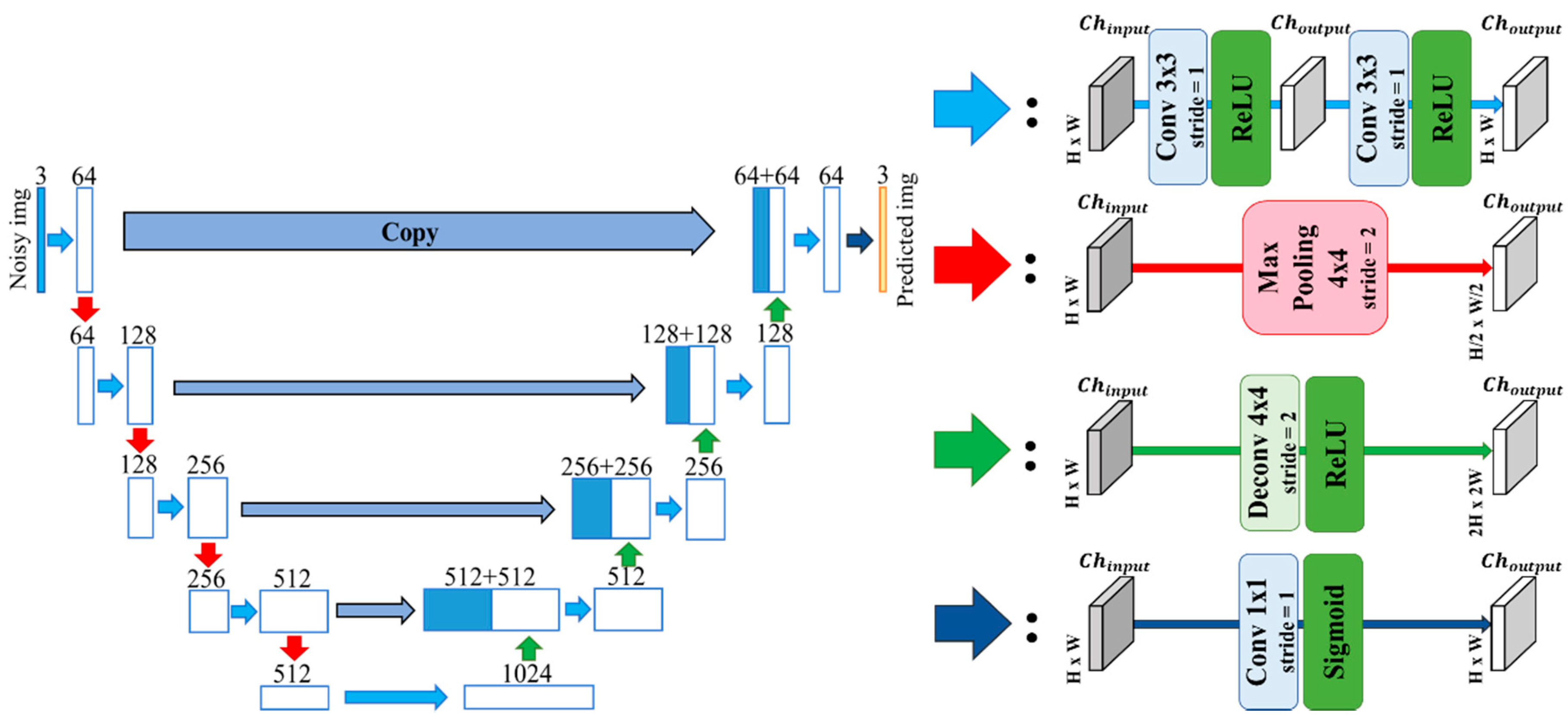
The original U-Net proposed by Ranneberger et al. [28] consists of the encoder with convolution layers called the contracting path and the decoder with up-convolution (deconvolution) layers called the expanding path. The U-Net also consists of the skip connections between the contracting path and expanding path. When up-sampling feature maps in the U-Net, the outputs from the previous deconvolution layer in the expanding path are concatenated with the feature maps obtained through the contracting path.
U-Net is widely used as the segmentation model in biomedical studies. For instance, Ronneberger et al. [28] utilized it in biomedical image segmentation in cells, Dong et al. [54] applied it to detect and segment brain tumors, and Çiçek et al. [55] proposed 3D U-Net which outputs 3D dense segmentation from the raw image directly.
Depending on how to expand the U-Net architecture, U-Net could be utilized to perform tasks other than segmentation. Isola et al. [30] employed U-Net as the generator and performed image-to-image translation task like aerial to map segmented labels to real objects, and grayscale images to color images through adversarial learning. Jansson et al. [56] adopted U-Net as a singing voice separator, whose input is the magnitude of the spectrogram of mixed audio. Zhang et al. [57] constructed U-Net with residual block as Residual U-Net and extracted the roads from aerial maps.
These related studies motivated us to investigate into the re-construction and application of U-Net architecture as a potential generalized denoising learner. Our study constructed the following three different denoising models based on the U-Net structure: Group Normalization U-Net, Residual U-Net, and Dense U-Net. Their structures and denoising functionality are described in the following sub-sections.
3.1. U-Net
3.2. U-Net with Group Normalization
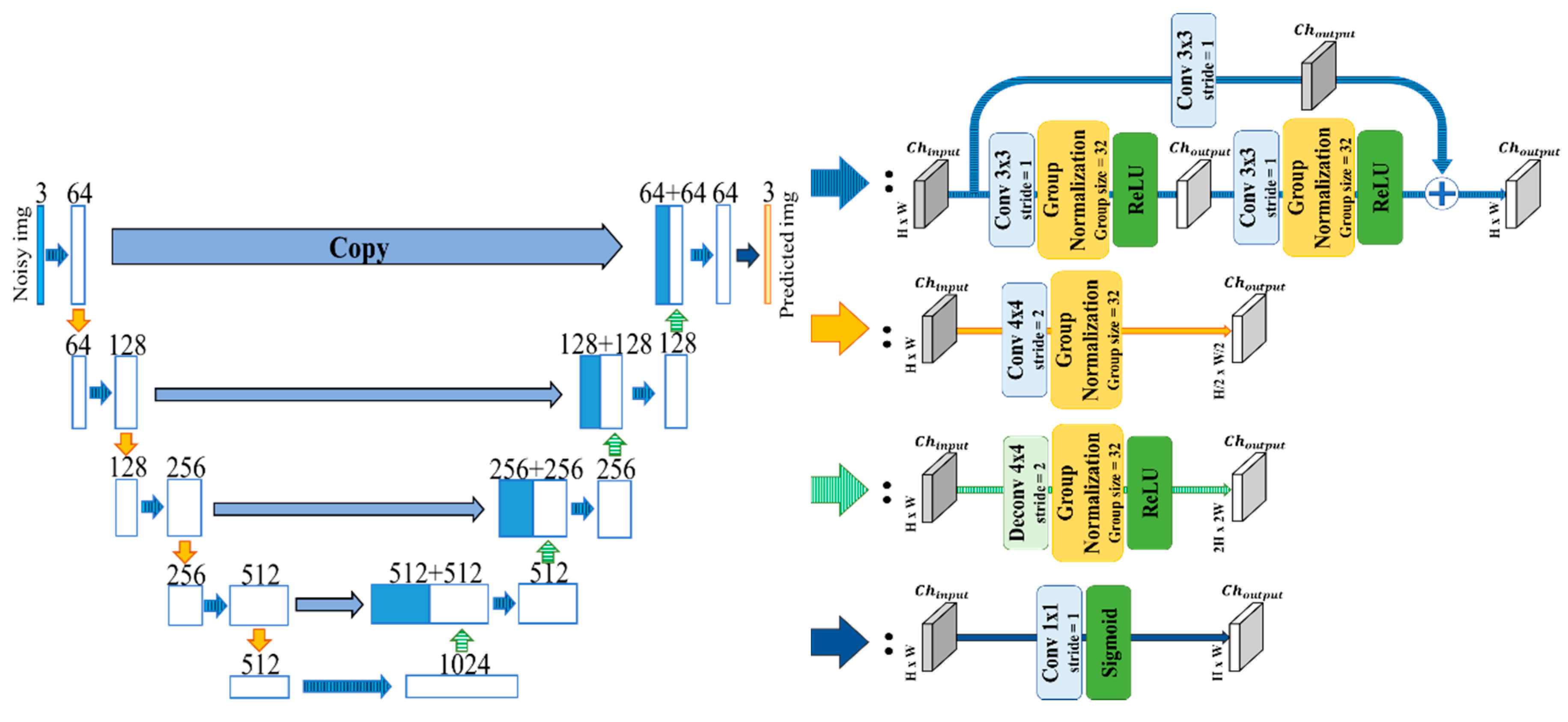
According to Santurkar et al. [58] introducing batch normalization in the training process makes the optimization smoother. However, batch normalization needs a sufficiently large batch size. We constructed the U-Net which adopted Batch Normalization and tried denoising after training. However, we found the results did not perform enough denoising in the testing phase because of the small batch size we set. Therefore, we employed the normalization called group normalization [29] and adopted it into each layer of the U-Net.
By contrast with batch normalization, group normalization sets the groups which consist of the divided channels of the feature map and normalizes depending on each group. This normalization does not need large batch size to accomplish the same results as the batch normalization. We call our U-Net with group normalization the U-Net with Gn (Figure 2). When implementing this model, we removed max pooling layers from the U-Net in Section 3.1 and adopted the group normalization whose channel size is 32 per group.
3.3. Residual U-Net
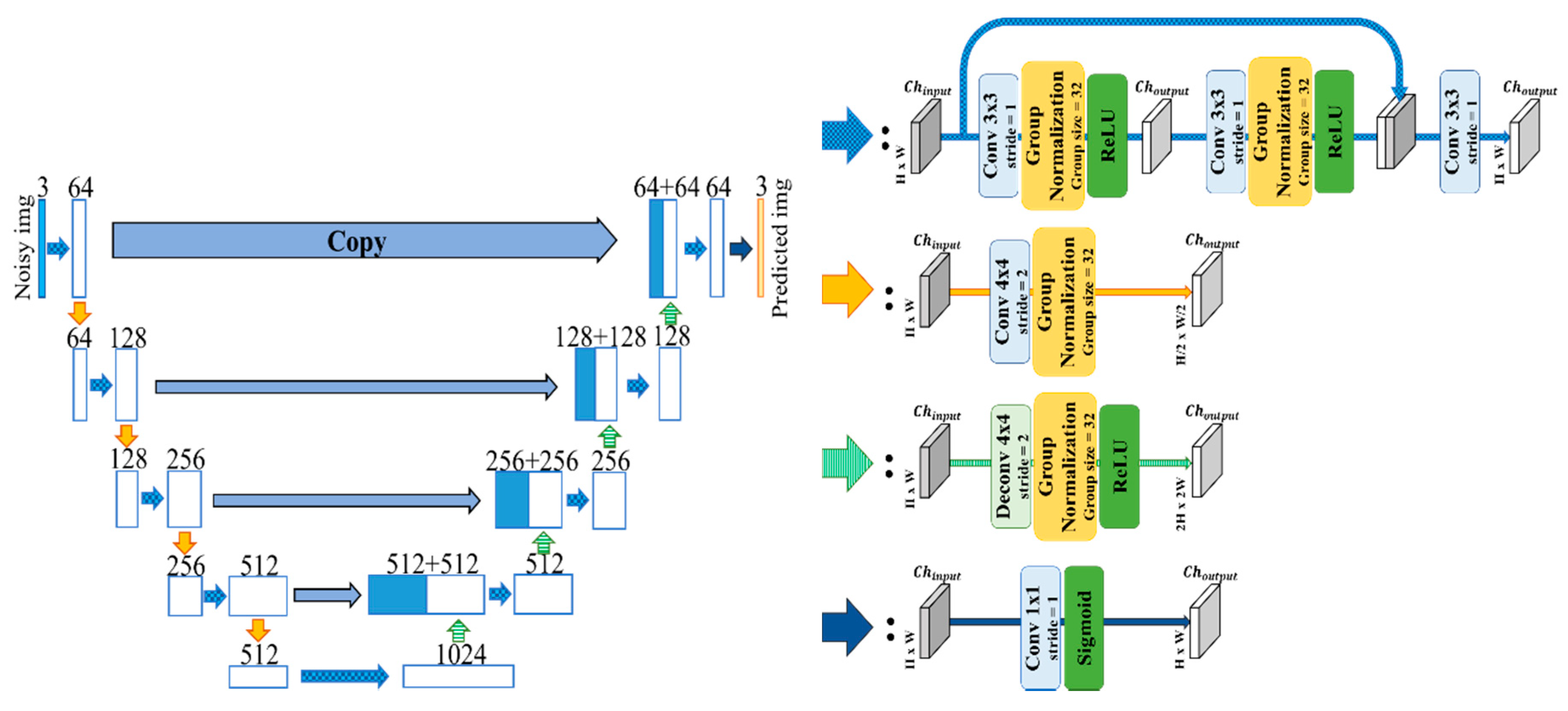
Zhang et al. point out that the U-Net is “lazy”, meaning that if the shallower layers in the U-Net learn enough in optimization, the deeper layers cannot obtain the gradient and learn well. This problem is the same as the degradation problem. To facilitate the propagation of the gradient information to the deeper layers, we employed residual learning architecture as in [59]. We adapted a residual block in each layer in the contracting as well as the expanding path of U-Net with Gn (Figure 3).
3.4. Dense U-Net
Huang et al. [60] have proposed DenseNet which connects by concatenating channels from the outputs of all the layers in order to obtain the maximum information flow along the layers. For comparing the shortcut connection differences between Residual Net and DenseNet, we adopt the element of DenseNet in our U-Net with Gn. According to the construction of DenseNet, this network stacks the outputs from the previous layer one by one and concatenates them. We tried adopting this process to U-Net with Gn, but found this structure takes a lot of time to complete a learning epoch. Therefore, we employed the structure which concatenates only the input when outputting and defined this network as Dense U-Net (Figure 4).
4. Loss Functions for Denoising
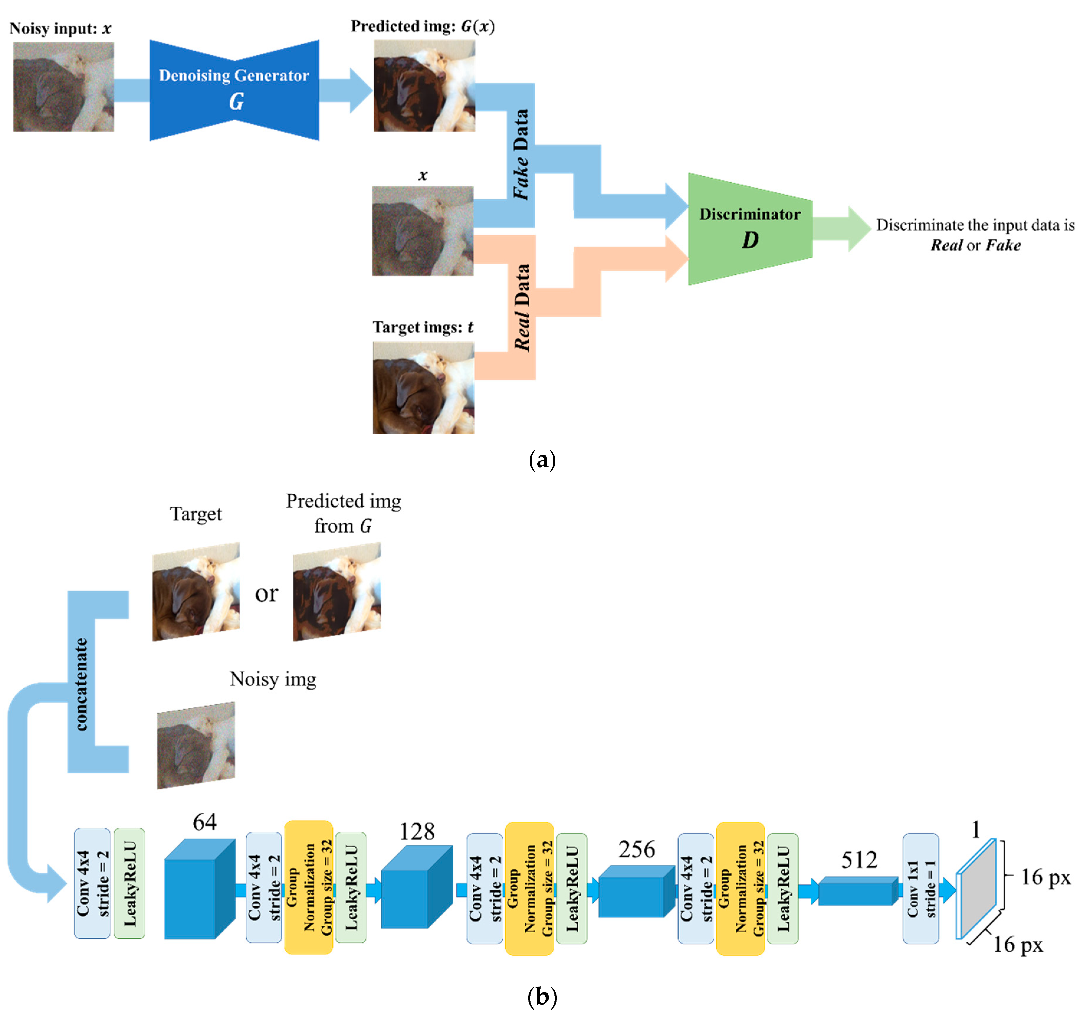
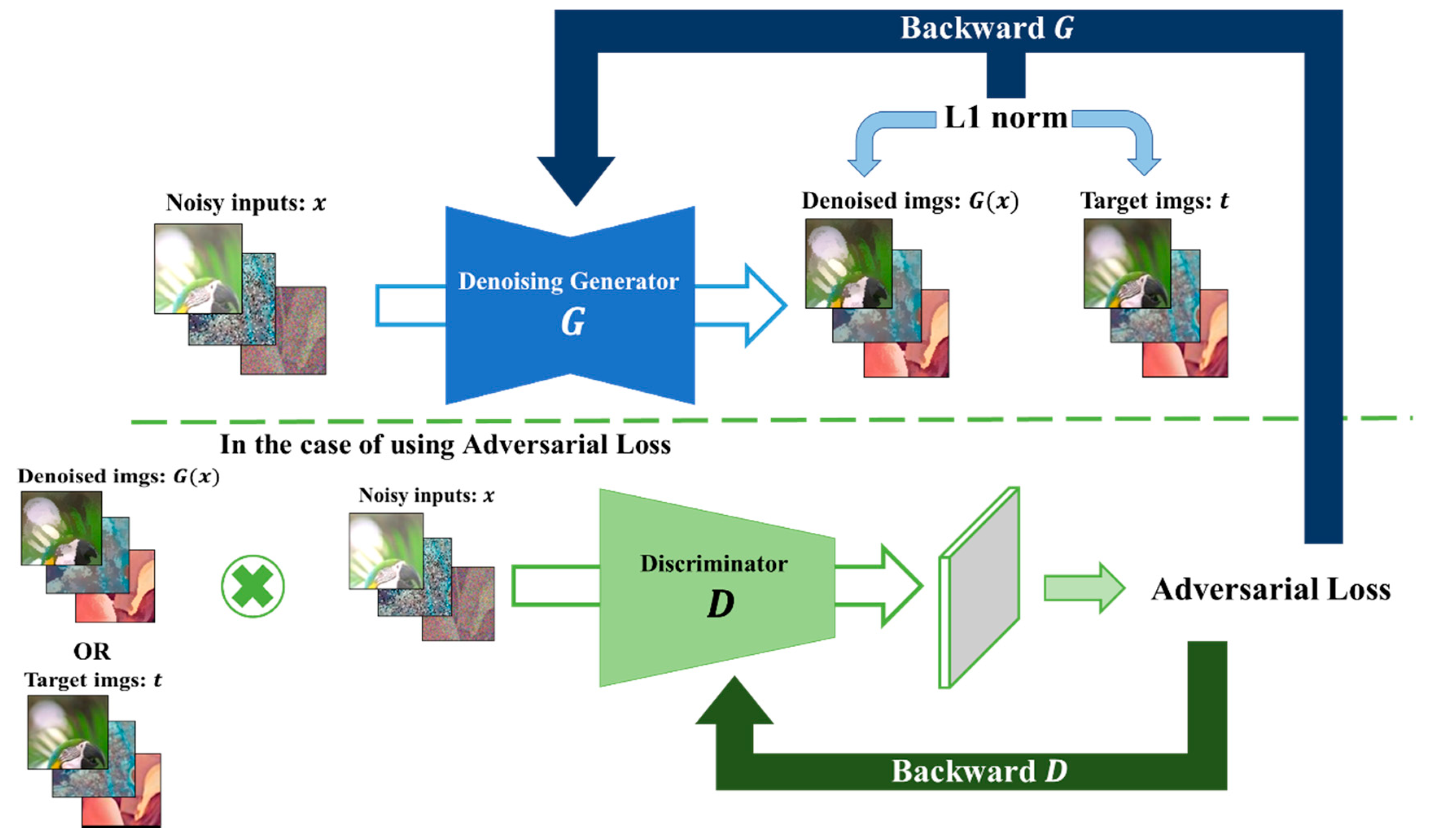
This section introduces the loss functions which are used in training for backpropagating each deep model. Our study employed two approaches: L1 norm and L1 norm + adversarial loss. To explain the loss functions, this section first gives an overview of the entire denoising learning structure (Figure 5a,b).
The deep learning model is a typical GAN, consisting of a denoising generator and a discriminator. For a particular model, the denoising generator contains one of the U-Net variants that we have described in the preceding section. Noisy images are fed to the generator which generates corresponding clean images. The discriminator is another deep network (Figure 5b) that learns to discriminate whether the clean image generated by the generator is real or fake.
In deep learning models, L1 or L2 regularizations (norms) are added to the loss function to overcome overfitting and improve the generalization of the model to any new test data [61]. The use of L1 and L2 norms, however, is by trial and error, depending on the image classification or reconstruction learning task. Pathak et al. [62] demonstrated that L2 produces blurry images, while Adversarial loss produces sharp images, but not coherent in experiments on inpainting—generating contents of an arbitrary image region conditioned on its surroundings. They obtained visually pleasing results by the combination of L2 and adversarial loss, which is computed from the outputs of G and D (Figure 5a).
Isola et al. [30] worked on the image translation problem, such as translating an aerial view of a map into street view, black and white images to color, daytime scenery to nighttime scenery, edges to full-color images, etc. They found that L1 with adversarial loss produces overall sharp and closer to ground-truth images. Our denoising task is a kind of translation, where we translate noisy images to clean images. Besides, L1 norm is found to be robust to outliers and noise compared to L2 norm [63]. Therefore, we adopted L1 norm with the intuition that robustness to outliers and noise can be useful since our model has to single-handedly deal with 5 different types of noises.
4.1. L1 Norm
In our denoising training, each denoising model aimed to output predicted images approximating clear targets from noisy inputs. Each model learned under the supervised learning with inputs and targets .
As the reconstruction loss to approximate targets, L1 norm was employed because of the robustness to outliers. The reconstruction objective can be expressed as:
To demonstrate that the strength of L1 norm affects denoising quality, we compared the models with reconstruction loss and .
4.2. L1 Norm + Adversarial Loss
The problem with L1 norm is that it is not an adequate objective function to output “sharp and clear” images, because the denoising model learns only from the difference distance. It has been demonstrated in [41] that the addition of adversarial loss leads to better performance than the model trained solely with L1 or L2 norm. Isola et al. [30] have proposed adversarial loss based on the patches from the output. After obtaining an N × N size output through the Discriminator , each patch is discriminated as real or fake (Patch GAN).
Our study suggests that Patch GAN might be an effective learning architecture since has the power to discriminate patches. We have employed Patch GAN expecting that the denoising model denoises in detail to deceive . The structure of our discriminator is shown in Figure 5b. Inputting the pair of images, the adversarial loss is obtained from 16 × 16 output patches by discriminating between the real—the input pair is the input (noisy image) and the target (ground truth image) and the fake—the input pair is the noisy input and the predicted image is from .
The objective can be expressed as:
When training the model with this adversarial loss, too, the scalar value of reconstruction loss is set to 100 and the weights of layers in the generator and discriminator are initialized from the Normal distribution with scale = 0.02.
5. Denoising Experiments
5.1. Dataset
For adding various types of noises on purpose, and for training our proposed denoising models through noisy images and evaluating their performance, we employed the ADE20K image dataset [64]. The ADE20K dataset is for semantic segmentation of the scenes in the images. The scenes are various, from inside of a room to outdoors and cityscapes. The total number of object classes in the images is larger than that in COCO [65] and ImageNet [66]. In our experiment, 20,210 images from the training set and 3352 images from the testing set were used for training and evaluation, respectively.
5.2. Image Pre-Processing
The computer vision library OpenCV was adopted for the pre-processing tasks like adding different kinds of noises and generating patches from the entire image. This section describes the kinds of noises that were generated, the parameters that were used for noise generation, and the arrangement of input and target data for training.
5.3. Adding Noise to Training Images at Random
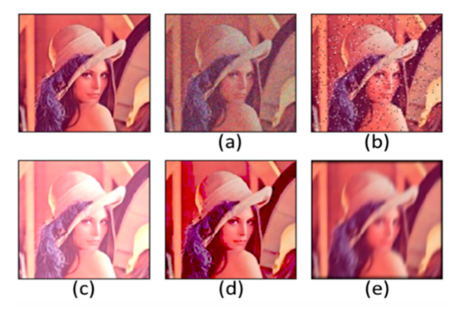
In generating noisy images as training set for denoising learning, each image in the training set of ADE20K was processed with a particular noise that was selected from 5 kinds of noise: Gaussian noise, salt-and-pepper noise, clipped whites, clipped blacks and camera shake. Gaussian noise and salt-and-pepper noise affect the texture of content image; clipped whites and clipped blacks enhance the strength of color and ruin the original color features, and camera shake makes the content image blurred because of unstable focus. An example of the processed images with their respective visual effects are shown in Figure 6. Some noises affect the brightness of the image, others clarity, and some others sharpness. Table 1 shows each type of noise with the respective hyperparameter.
5.4. Generating Patches from the Image
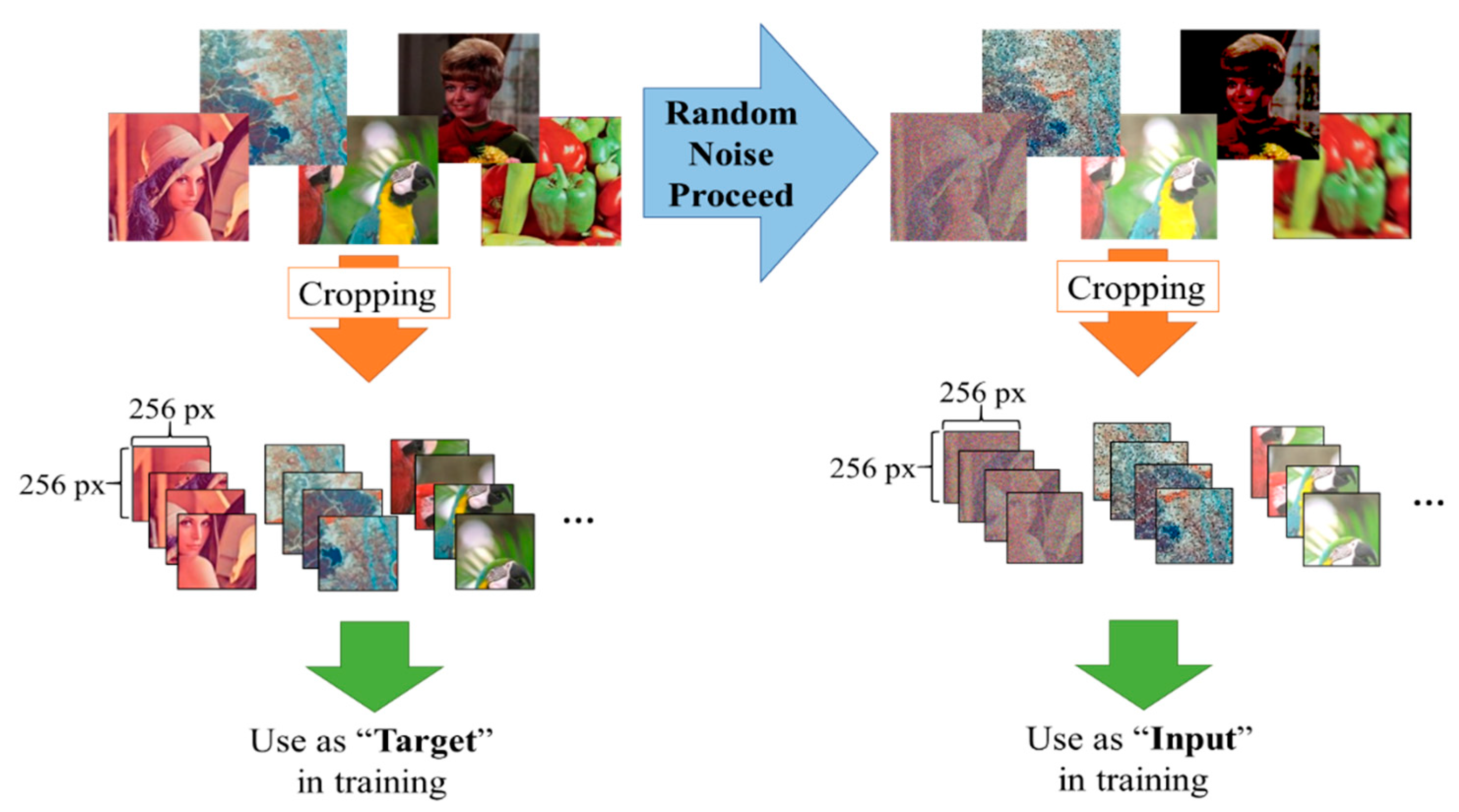
To handle different sizes of the input images, we cropped them to 256 × 256 patch sizes of the input image (the processed noisy image) and the target image (the image before processing). The process to generate these patches is illustrated in Figure 7. Repeating the cropping procedure on the images from the training set, we collected 90,067 patches from 20,120 images. The input patches serve as inputs to the deep denoising model and the target patches as supervised data. The patches which were output from the deep denoising model were then gathered and assembled to reconstruct the entire predicted image.
5.5. Denoising Training Implementation
We implemented denoising learning with the deep-learning framework called chainer [67]. The network was trained on two NVIDIA GeForce RTX 2080 Ti (11 GB) GPUs. In the training phase, each model learned blind denoising with 90,067 training patches for 30 epochs with batch size = 5 and Adam optimization function. The hyperparameters of Adam were: L1 norm loss; learning rate and the exponential rate of momentum, . On the other hand, for the training adopting L1 norm + adversarial loss, we set and for stable learning between the Generator and the Discriminator.
The overview of the denoising training process is described in Figure 8. When training only the denoising generator the algorithm goes through the following steps (S):
- S1.
- Input the noisy images to .
- S2.
- Get the predicted denoised output images .
- S3.
- Compute L1 norm loss by comparing and clean target images .
- S4.
- Train the parameters of through backpropagation.
On the other hand, when training denoising including adversarial learning, we trained denoising generator and discriminator in the following steps (S):
- S1.
- Input to .
- S2.
- Using , input the pair of data to and get adversarial loss from by comparing with the real label.
- S3.
- Adopting L1 norm and adversarial loss as the total loss of , backpropagate and
- S4.
- update the parameters of .Input pairs of fake data and real data , to .
- S5.
- Calculate adversarial loss by comparing with fake label and with
- S6.
- real label. Adopting adversarial loss in Step5 as the total loss of , backpropagate and update the parameters of .
6. Results
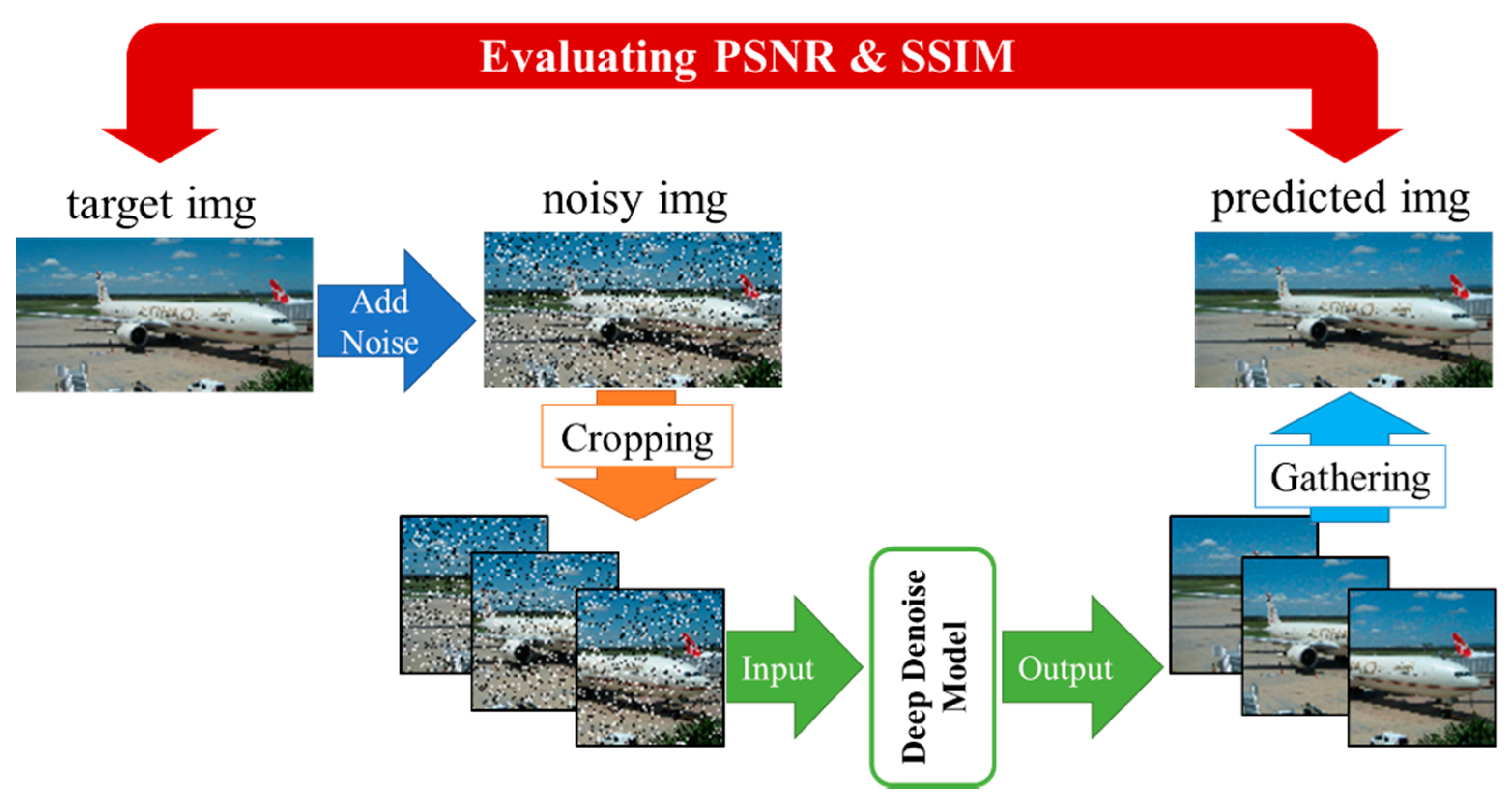
After denoising learning using each model, we evaluated the quality of denoising results with the test dataset images that we introduced in Section 5. As criteria for denoising evaluation, we employed PSNR for image quality assessment and SSIM for the similarity evaluation between the ground truth image and the predicted image. The evaluation procedure is shown in Figure 9.
Evaluating PSNR and SSIM in our model is done as follows:
- S1.
- Input a clean test image and use it as a target image.
- S2.
- Add noise to target image and use it as noisy image.
- S3.
- Crop the noisy image to 256 × 256 size.
- S4.
- Input the noisy cropped images to the deep denoising model, and obtain de-noised cropped images.
- S5.
- Collected cropped output images from the model. Patch them together to form the denoised predicted image.
- S6.
- Evaluate the predicted image using PSNR and SSIM compared to the target image.
Section 6.1, Section 6.2, Section 6.3, Section 6.4 and Section 6.5 below explain the denoising results obtained by using the testing dataset to which specific noise parameters were added on purpose. For comparing with the related studies of denoising, we also constructed and trained DnCNN [38] and WIN5RB [68] using the same training dataset mentioned in Section 5. The best results in each table are shown in boldface.
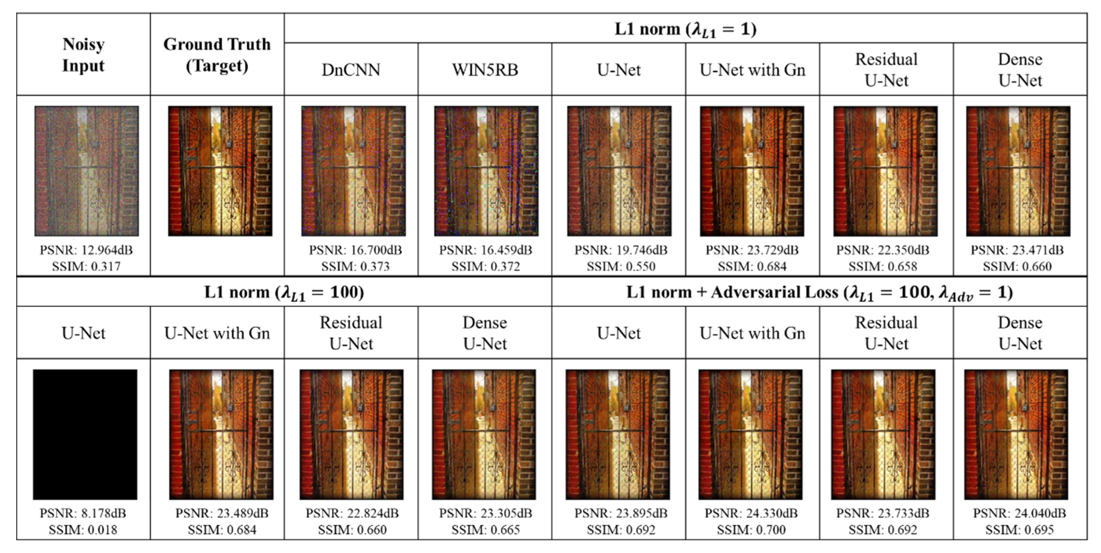
6.1. Denoising Results: Gaussian Noise
Table 2 shows the average values of PSNR and SSIM using the test dataset setting the Gaussian noise parameter as and 80. Figure 10 shows the denoised images after inputting the noisy input image with to each trained model. The best results are in boldface. Our expanded U-Nets, namely, U-Net with Gn, Residual U-Net and Dense U-Net trained through each of the loss objectives could improve PSNR and SSIM for every noise level compared to DnCNN, WIN5RB and U-Net. The U-Net with L1 norm ( recorded the worst PSNR and SSIM because of the disruption in the training phase (the loss suddenly began to increase). In Figure 10, U-Net with Gn, Residual U-Net and Dense U-Net succeeded in increasing PSNR over 20.0 dB and hardly left behind any vestiges of the Gaussian noise.
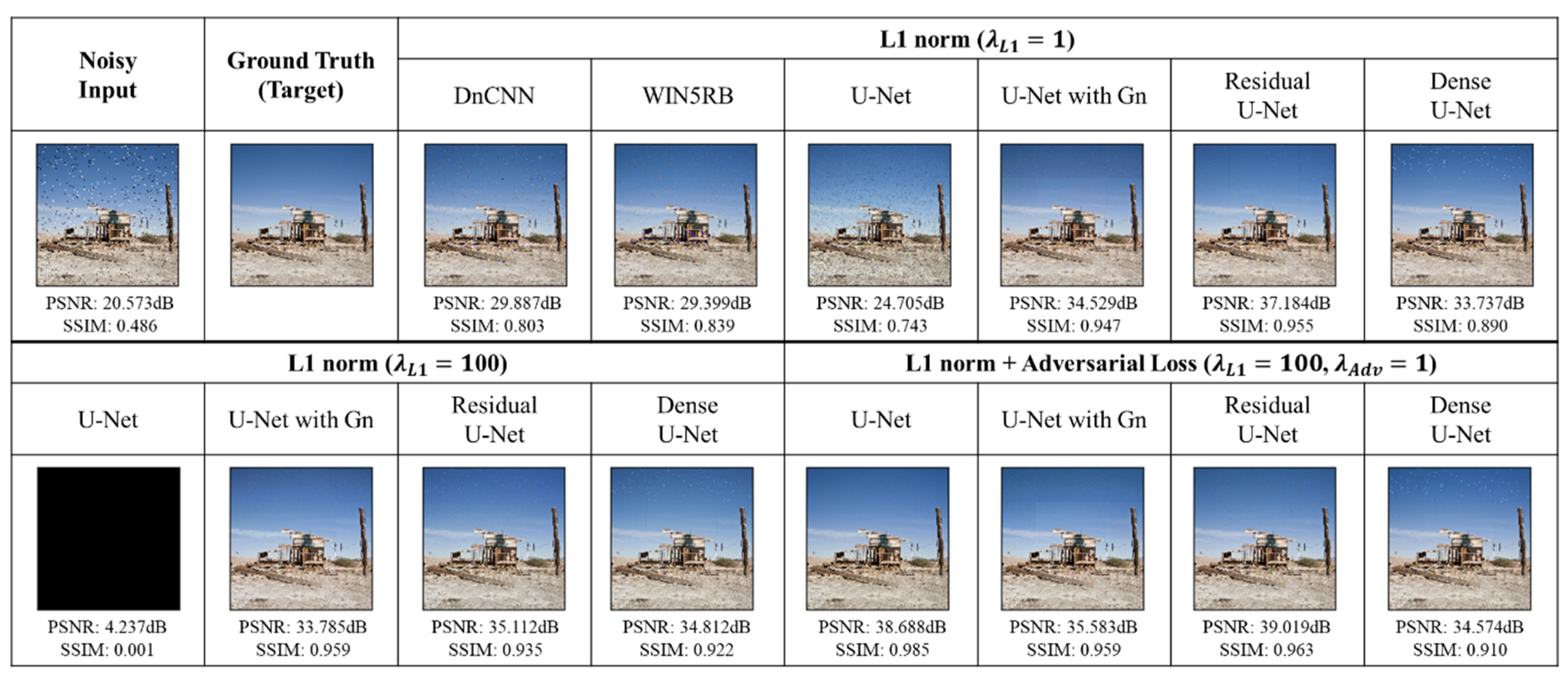
6.2. Denoising Results: Salt-and-Pepper Noise
Table 3 shows the average values of PSNR and SSIM with the salt-and-pepper noise parameter as and 0.3. Figure 11 shows the denoised images after inputting the noisy input image to each trained model. Almost all U-Net models could improve noisy images to over 25 dB. The U-Net with L1 norm + adversarial loss marked the best result, although by a narrow margin. In Figure 11, each result appears to be adequately cleared of the salt-and-pepper noise.
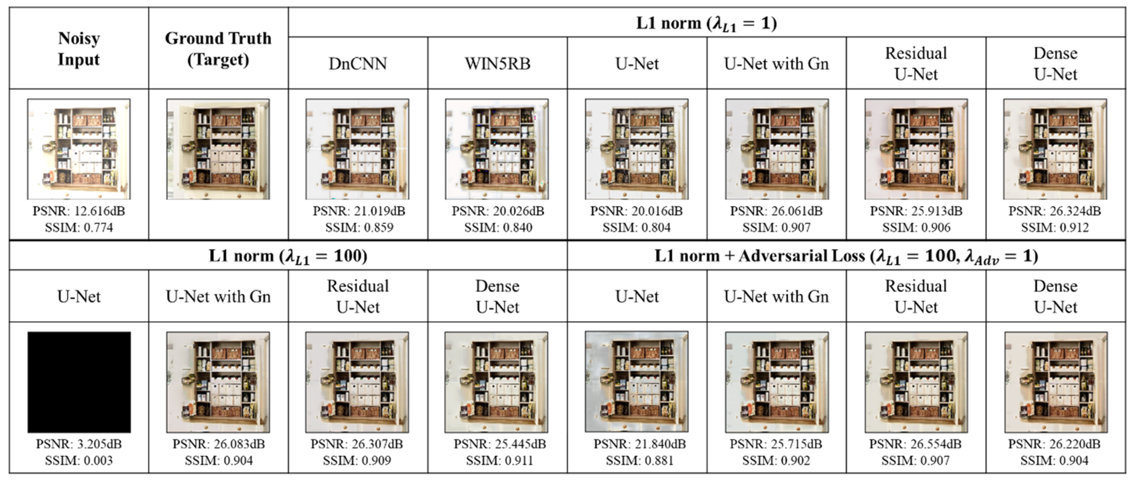
6.3. Denoising Results: Clipped Whites
Table 4 shows the average of PSNR and SSIM for the test dataset with the parameter of clipped whites as and 100. Figure 12 shows the denoised images after inputting the noisy input image with to each trained model. U-Net with Gn, Residual U-Net and Dense U-Net contributed to improve the average results of PSNR and SSIM for both the loss objectives. As seen in the visualized results in Figure 12, the over-lit noisy image was denoised so that the shape of the objects appears very clear. Moreover, all our three models (U-Net with Gn, Residual U-Net and Dense U-Net) showed excellent performance. Their SSIM value peaked near 0.9 whatever the loss objective.
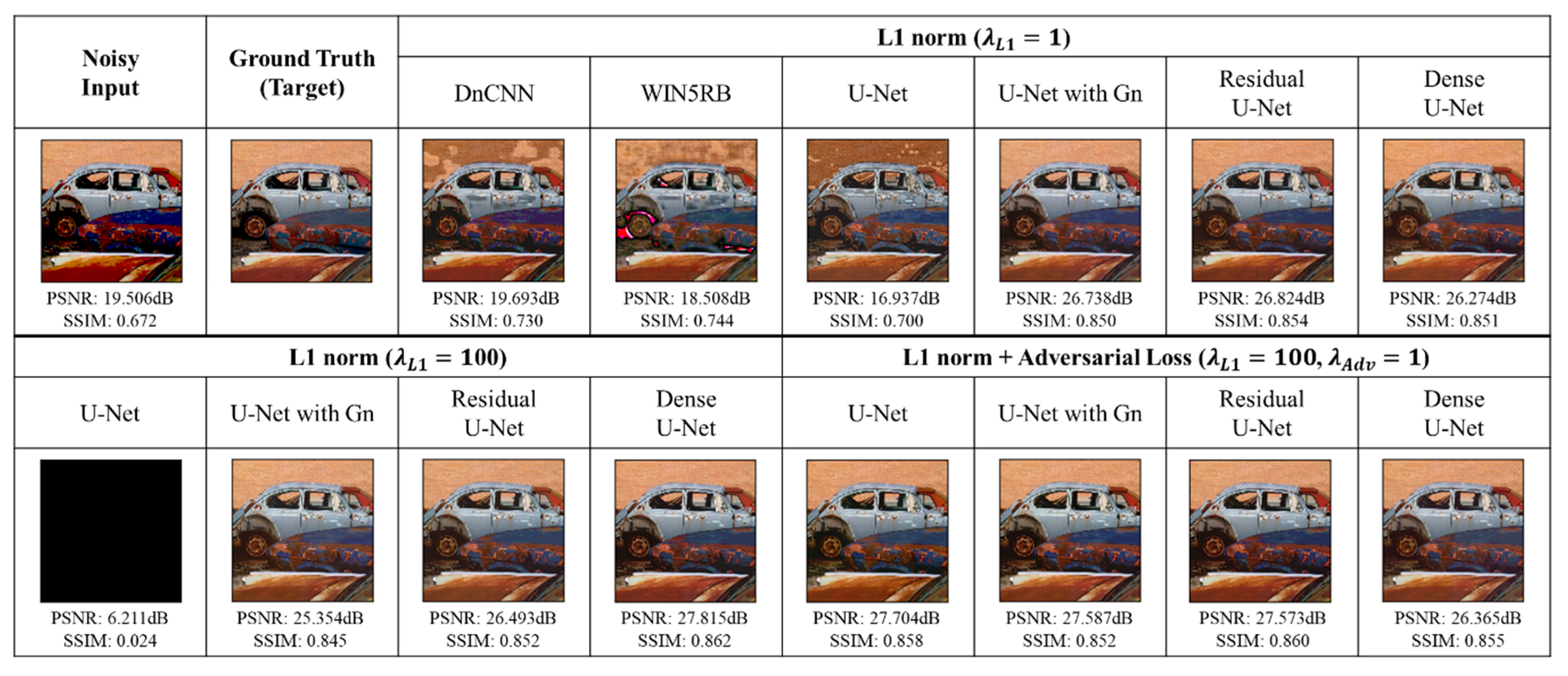
6.4. Denoising Results: Clipped Blacks
Table 5 shows the average of PSNR and SSIM for the test dataset with the parameter of clipped blacks as and 100. Figure 13 shows the denoised images after inputting the noisy input image with to each trained model. As shown in Table 5, the Residual U-Net and Dense Net with L1 norm + adversarial loss output the best PSNR and SSIM. As for the visualized output results, DnCNN, WIN5RB and U-Net with L1 norm () left the wrong color in some objects. On the other hand, those models that produced PSNR larger than 25.0 dB could handle the color compensation wherever necessary.
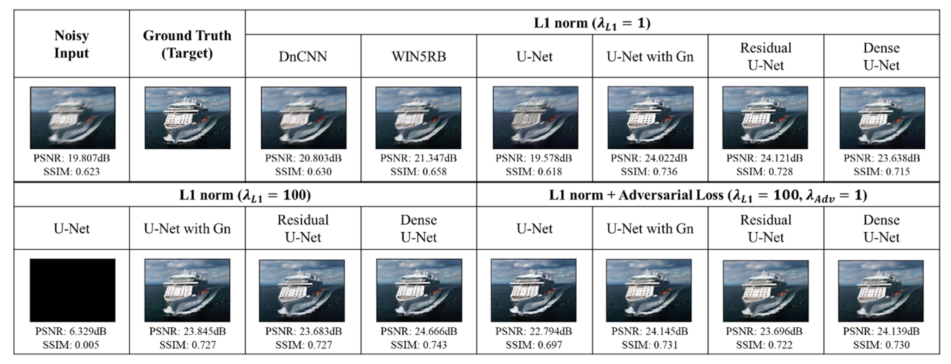
6.5. Denoising Results: Camera Shake
Table 6 shows the average PSNR and SSIM results of the different denoising models for camera shake with and . Figure 14 shows the denoised images after inputting the noisy input image to each trained model. In Table 6, the Dense U-Net with L1 norm () shows better PSNR and SSIM than the one with L1 norm + adversarial loss. In the visualized results of Figure 14 the models which have achieved PSNR greater than 24.0 dB make the blurred noisy image clear, rendering the detailed objects in the image comprehensible.
6.6. Comparing the U-Net Based Model’s Denoisng Perfromace with Standard Models
Table 7 shows the denoising performance of our model compared with that of some standard models. The table is divided into 5 sections vertically, each section dealing with the PSNR values for a particular type of noise. Peak signal-to-noise ratio (PSNR) is the ratio of the maximum possible power of a signal to the power of corrupting noise that affects the fidelity of its representation. Higher values of PSNR generally indicate that the reconstruction is of higher quality.
The first row in each section of the table shows the level of noise we have added to each experimental input image. The noise levels for experimentation are also shown in Table 1 above. The second row shows the PSNR value computed with the added noise. The next two rows show the PSNR performance values of the DnCNN and WIN5RB models, respectively. In all the sections, some variant of our U-Net based model shows the best results, which are far above those produced by the above two standard models. As seen from the visualized output results (Figure 10, Figure 11, Figure 12, Figure 13 and Figure 14), our models produced sharper and clearer denoised images than those produced by the standard U-net, DnCNN, and WIN5RB.
The table shows a comparison in the performance of our three variants. Residual U-Net and Dense U-Net tend to be robust in denoising different kinds of noise. Secondly, comparing the quality of the loss objectives, the L1 norm summed with adversarial loss output higher PSNR values than the simple L1 norm.
7. Conclusions
Due to the influence of sensors, transmission channels, and other factors, digital images are invariably corrupted by noise during the process of acquisition, compression, storage, and transmission. The presence of subtle noise leads to distortion and information loss adversely affecting the subsequent image processing tasks such as analysis, recognition, and tracking. Noise removal goes much further than just beautifying images. The success of image processing like face recognition, biometric security, remote sensing, object detection and recognition in autonomous driving, and medical imaging rests on extremely high-quality images. Therefore, image denoising plays an important role in modern image processing systems.
Several techniques for noise removal are well established in color image processing. While most of the algorithms act as filters or wavelength transforms, we present a state-of-the-art deep-learning model for denoising. Furthermore, most conventional models are designed for specific noise like Gaussian or salt-and-pepper.
The study describes the architectures and functionalities of three types of deep-learning denoising models, all based on the standard segmentation U-Net: (1) U-Net with Group Normalization, (2) Residual U-Net with shortcuts applied to the decoder/encoder, and (3) Dense U-Net with concatenation of input/output feature maps to the decoder/encoder. All the three models adopt group normalization and convolution in place of max pooling. The error function used for learning is not a simple L1 norm, but L1 norm with stronger coefficients. In addition, L1 norm + patch loss is also used. After extensive comparative experiments of noise removal, Residual U-Net and Dense U-Net with L1 norm + Patch loss function were found to be robust and superior in performance.
The advantage of our model is that it is adaptive and can handle five different types of known noise in digital images. Furthermore, no additional information about the noise type is necessary while training the model as in the case of most denoising models. All the three variants outperform the existing noise reduction models like DnCNN and WIN5RB evaluated by means of the PSNR/SSIM metrics.
Although the purpose of this study has been satisfactorily achieved, there are limitations, too. First, our noise-removal approach is based on supervised learning. To achieve this, we need paired data of the input noisy image and the corresponding clean target image. In real-life situations, there is hardly any dataset containing pairs of noisy/clean images. Most datasets contain only noisy images without their clean counterparts. In such cases, learning using the L1 norm between the noise-removed image and the target clean image is not feasible. To cope with such situations, it is necessary to try unsupervised learning using unpaired datasets such as the CycleGAN architecture [69]. Second, our model was trained for removal of noise such as salt-and-pepper noise and camera shake that can be visually verified by human subjects. However, there exist other kinds of noise that are feeble and almost invisible. The latest adversarial attack security breaches on digital images is one such feeble and invisible noise. Our model is effective against strong visible noise, but not for detecting weak and invisible noise. To overcome such a defect, it is necessary to approach the denoising learning with datasets including invisible weak noise.
The accuracy of current state-of-the-art pattern recognition and deep-learning algorithms for object detection and recognition is limited by the noise factor. It is expected that by passing the images through the denoising model developed in our research, features with strong noise can be reduced and accurate object recognition and detection from images can be performed. The precision and applicability of our core denoising model can be enhanced by means of further learning using larger datasets and transfer learning.
Author Contributions
Both the authors are engaged in a collaborative research in the Gonsalves AI lab (https://www.gonken.tokyo/), Department of Information & Communication Sciences, Sophia University, Tokyo, Japan. R.K., a PhD student, conceived the original idea of denoising RGB images. Both the authors discussed the viability and the contribution of the deep learning model to denoising images. R.K., who is well-versed with U-net, constructed three variants of the model, coded the programs, executed them on GPUs and produced promising results after several months. She then wrote the first draft of the manuscript. T.G., the research director, checked the results, collected related studies in denoising images, and wrote the final draft of the paper adding more content and references. The authors also had several discussions together to make revisions to the original manuscript and respond to the reviewers’ queries. T.G. made changes to the structure and content of the original manuscript, citing additional related references. R.K. added more figures and checked the minute details. Both the authors worked equally on the second revision and on the final camera-ready version of the paper. Both authors have read and agreed to the published version of the manuscript.
Funding
This research received no external funding.
Conflicts of Interest
The authors declare no conflict of interest.
References
- Li, Y.; Zhang, B.; Florent, R. Understanding neural-network denoisers through an activation function perspective. In Proceedings of the IEEE International Conference on Image Processing (ICIP), Beijing, China, 17–20 September 2017. [Google Scholar]
- Burger, H.C.; Schuler, C.J.; Harmeling, S. Image denoising: Can plain Neural Networks compete with BM3D? In Proceedings of the IEEE Conference on Computer Vision and Pattern Recognition, Providence, Rhode Island, 16–21 June 2012.
- Abubakar, A.; Zhao, X.; Li, S.; Takruri, M.; Bastaki, E.; Bermak, A. A Block-Matching and 3-D Filtering Algorithm for Gaussian Noise in DoFP Polarization Images. IEEE Sens. J. 2018, 18, 7429–7435. [Google Scholar] [CrossRef]
- Rabbouch, H.; Saâdaoui, F.; Vasilakos, A.V. A wavelet-assisted subband denoising for tomographic image reconstruction. J. Vis. Commun. Image Represent. 2018, 55, 115–130. [Google Scholar] [CrossRef]
- Kaur, G.; Kaur, R. Image De-Noising using Wavelet Transform and Various Filters. Int. J. Res. Comput. Sci. 2012, 2, 15–21. [Google Scholar] [CrossRef]
- Song, Q.; Ma, L.; Cao, J.; Han, X. Image Denoising Based on Mean Filter and Wavelet Transform. In Proceedings of the 4th International Conference on Advanced Information Technology and Sensor Application (AITS), Harbin, China, 21–23 August 2015. [Google Scholar]
- Vyas, A.; Paik, J. Applications of multiscale transforms to image denoising: Survey. In Proceedings of the International Conference on Electronics, Information, and Communication (ICEIC), Honolulu, HI, USA, 24–27 January 2018. [Google Scholar]
- Bhonsle, D.; Chandra, V.; Sinha, G. Medical Image Denoising Using Bilateral Filter. Int. J. Image Graph. Signal Process. 2012, 4, 36–43. [Google Scholar] [CrossRef] [Green Version]
- Kumar, B.K.S. Image denoising based on gaussian/bilateral filter and its method noise thresholding. Signal Image Video Process. 2012, 7, 1159–1172. [Google Scholar] [CrossRef]
- Sarker, S. Use of Non-Local Means Filter to Denoise Image Corrupted by Salt and Pepper Noise. Signal Image Process. Int. J. 2012, 3, 223–235. [Google Scholar] [CrossRef]
- Gacsadi, A.; Szolgay, P. Variational computing based images denoising methods by using cellular neural networks. In Proceedings of the European Conference on Circuit Theory and Design, Antalya, Turkey, 23–27 August 2009. [Google Scholar]
- Lim, B.; Son, S.; Kim, H.; Nah, S.; Lee, K.M. Enhanced Deep Residual Networks for Single Image Super-Resolution. In Proceedings of the IEEE Conference on Computer Vision and Pattern Recognition Workshops (CVPRW), Honolulu, HI, USA, 21–26 July 2017. [Google Scholar]
- Liu, D.; Wen, B.; Fan, Y.; Loy, C.C.; Huang, T.S. Non-Local Recurrent Network for Image Restoration. Adv. Neural Inf. Process. Syst. 2018, 2018-December, 1673–1682. [Google Scholar]
- Krizhevsky, A.; Sutskever, I.; Hinton, G.E. ImageNet classification with deep convolutional neural networks. In Proceedings of the Advances in Neural Information Processing Systems (NIPS), Lake Tahoe, NV, USA, 3–6 December 2012. [Google Scholar]
- Dargan, S.; Kumar, M.; Ayyagari, M.R.; Kumar, G. A Survey of Deep Learning and Its Applications: A New Paradigm to Machine Learning. Arch. Comput. Methods Eng. 2019, 27, 1071–1092. [Google Scholar] [CrossRef]
- Simonyan, K.; Zisserman, A. Very Deep Convolutional Networks for Large-Scale Image Recognition. arXiv 2014, arXiv:1409.1556. Available online: https://arxiv.org/abs/1409.1556 (accessed on 1 May 2020).
- Ren, S.; He, K.; Girshick, R.; Sun, J. Faster R-CNN: Towards real-time object detection with region proposal networks. Adv. Neural Inf. Process. Syst. 2015, 1, 91–99. [Google Scholar] [CrossRef] [Green Version]
- Redmon, J.; Divvala, S.; Girshick, R.; Farhadi, A. You only look once: Unified, real-time object detection. In Proceedings of the IEEE Conference on Computer Vision and Pattern Recognition, Las Vegas, NV, USA, 27–30 June 2016; pp. 779–788. [Google Scholar]
- Galea, C.; Farrugia, R.A. Matching Software-Generated Sketches to Face Photographs With a Very Deep CNN, Morphed Faces, and Transfer Learning. IEEE Trans. Inf. Forensics Secur. 2017, 13, 1421–1431. [Google Scholar] [CrossRef]
- Ranjan, R.; Patel, V.M.; Chellappa, R. HyperFace: A Deep Multi-Task Learning Framework for Face Detection, Landmark Localization, Pose Estimation, and Gender Recognition. IEEE Trans. Pattern Anal. Mach. Intell. 2017, 41, 121–135. [Google Scholar] [CrossRef] [PubMed] [Green Version]
- Kumar, A.; Kim, J.; Lyndon, D.; Fulham, M.; Feng, D. An Ensemble of Fine-Tuned Convolutional Neural Networks for Medical Image Classification. IEEE J. Biomed. Heal. Inf. 2016, 21, 31–40. [Google Scholar] [CrossRef] [PubMed] [Green Version]
- Chandra, B.S.; Sastry, C.S.; Jana, S. Robust Heartbeat Detection from Multimodal Data via CNN-Based Generalizable Information Fusion. IEEE Trans. Biomed. Eng. 2018, 66, 710–717. [Google Scholar] [CrossRef] [PubMed] [Green Version]
- Tian, C.; Fei, L.; Zheng, W.; Xu, Y.; Zuo, W.; Lin, C.-W. Deep learning on image denoising: An overview. Neural Netw. 2020, 131, 251–275. [Google Scholar] [CrossRef] [PubMed]
- Dodge, S.; Karam, L. Understanding how image quality affects deep neural networks. In Proceedings of the Eighth International Conference on Quality of Multimedia Experience (QoMEX), Lisbon, Portugal, 6–8 June 2016. [Google Scholar]
- Nazaré, T.S.; Da Costa, G.B.P.; Contato, W.A.; Ponti, M.A. Deep Convolutional Neural Networks and Noisy Images. In Lecture Notes in Computer Science; Springer Science and Business Media LLC: Berlin/Heidelberg, Germany, 2018; pp. 416–424. [Google Scholar]
- Eykholt, K.; Evtimov, I.; Fernandes, E.; Li, B.; Rahmati, A.; Xiao, C.; Prakash, A.; Kohno, T.; Song, D. Robust Physical-World Attacks on Deep Learning Visual Classification. In Proceedings of the IEEE/CVF Conference on Computer Vision and Pattern Recognition, Salt Lake City, UT, USA, 18–23 June 2018. [Google Scholar]
- Lucas, A.; Iliadis, M.; Molina, R.; Katsaggelos, A.K. Using Deep Neural Networks for Inverse Problems in Imaging: Beyond Analytical Methods. IEEE Signal Process. Mag. 2018, 35, 20–36. [Google Scholar] [CrossRef]
- Ronneberger, O.; Fischer, P.; Brox, T. U-net: Convolutional networks for biomedical image segmentation. In International Conference on Medical Image Computing and Computer-Assisted Intervention; Springer: New York, NY, USA, 2015; pp. 234–241. [Google Scholar]
- Wu, Y.; He, K. Group Normalization. Int. J. Comput. Vis. 2019, 128, 742–755. [Google Scholar] [CrossRef]
- Isola, P.; Zhu, J.-Y.; Zhou, T.; Efros, A.A. Image-to-Image Translation with Conditional Adversarial Networks. In Proceedings of the IEEE Conference on Computer Vision and Pattern Recognition (CVPR), Honolulu, HI, USA, 21–26 July 2017. [Google Scholar]
- Hinton, G. Reducing the Dimensionality of Data with Neural Networks. Science 2006, 313, 504–507. [Google Scholar] [CrossRef] [Green Version]
- Gondara, L. Medical Image Denoising Using Convolutional Denoising Autoencoders. In Proceedings of the IEEE 16th International Conference on Data Mining Workshops (ICDMW); Institute of Electrical and Electronics Engineers (IEEE), Barcelona, Spain, 12–15 December 2016. [Google Scholar]
- Xiang, Q.; Pang, X. Improved Denoising Auto-Encoders for Image Denoising. In Proceedings of the 11th International Congress on Image and Signal Processing, BioMedical Engineering and Informatics (CISP-BMEI), Beijing, China, 13–15 October 2018. [Google Scholar]
- Ghose, S.; Singh, N.; Singh, P. Image Denoising using Deep Learning: Convolutional Neural Network. In Proceedings of the 10th International Conference on Cloud Computing, Data Science & Engineering (Confluence), Noida, India, 29–31 January 2020. [Google Scholar]
- Li, X.; Xiao, J.; Zhou, Y.; Ye, Y.; Lv, N.; Wang, X.; Wang, S.; Gao, S. Detail retaining convolutional neural network for image denoising. J. Vis. Commun. Image Represent. 2020, 71, 102774. [Google Scholar] [CrossRef]
- Esser, P.; Sutter, E. A Variational U-Net for Conditional Appearance and Shape Generation. In Proceedings of the IEEE/CVF Conference on Computer Vision and Pattern Recognition, Salt Lake City, UT, USA, 18–22 June 2018. [Google Scholar]
- Komatsu, R.; Gonsalves, T. Effectiveness of U-Net in Denoising RGB Images. Comput. Sci. Inf. Techn. 2019, 1–10. [Google Scholar] [CrossRef]
- Zhang, K.; Zuo, W.; Chen, Y.; Meng, D.; Zhang, L. Beyond a Gaussian Denoiser: Residual Learning of Deep CNN for Image Denoising. IEEE Trans. Image Process. 2017, 26, 3142–3155. [Google Scholar] [CrossRef] [PubMed] [Green Version]
- He, K.; Zhang, X.; Ren, S.; Sun, J. Deep Residual Learning for Image Recognition. In Proceedings of the 2016 IEEE Conference on Computer Vision and Pattern Recognition (CVPR); Institute of Electrical and Electronics Engineers (IEEE), Las Vegas, NV, USA, 27–30 June 2016; pp. 770–778. [Google Scholar]
- Ioffe, S.; Szegedy, C. Batch Normalization: Accelerating Deep Network Training by Reducing Internal Covariate Shift. arXiv 2015, arXiv:1502.03167. [Google Scholar]
- Goodfellow, I.J.; Pouget-Abadie, J.; Mirza, M.; Xu, B.; Warde-Farley, D.; Ozair, S.; Courville, A.; Bengio, Y. Generative Adversarial Nets. Adv. Neural Inf. Process. Syst. 2014, arXiv:1406.2661v1, 2672–2680. [Google Scholar]
- Yang, L.; Shangguan, H.; Zhang, X.; Wang, A.; Han, Z. High-Frequency Sensitive Generative Adversarial Network for Low-Dose CT Image Denoising. IEEE Access 2020, 8, 930–943. [Google Scholar] [CrossRef]
- Park, H.S.; Baek, J.; You, S.K.; Choi, J.K.; Seo, J.K. Unpaired Image Denoising Using a Generative Adversarial Network in X-Ray CT. IEEE Access 2019, 7, 110414–110425. [Google Scholar] [CrossRef]
- Alsaiari, A.; Rustagi, R.; Alhakamy, A.; Thomas, M.M.; Forbes, A.G. Image Denoising Using A Generative Adversarial Network. In Proceedings of the IEEE 2nd International Conference on Information and Computer Technologies (ICICT), Kahului, HI, USA, 13–17 March 2019. [Google Scholar]
- Gopan, K.; Kumar, G. Video Super Resolution with Generative Adversarial Network. In Proceedings of the 2nd International Conference on Trends in Electronics and Informatics (ICOEI), Tiruneveli, India, 11–12 May 2018. [Google Scholar]
- López-Tapia, S.; Lucas, A.; Molina, R.; Katsaggelos, A.K. A single video super-resolution GAN for multiple downsampling operators based on pseudo-inverse image formation models. Digit. Signal Process. 2020, 104, 102801. [Google Scholar] [CrossRef]
- Bell-Kligler, S.; Shocher, A.; Irani, M. Blind super-resolution kernel estimation using an internal-GAN. Adv. Neural Inf. Process. Syst. 2019, 1, 284–293. [Google Scholar]
- Ledig, C.; Theis, L.; Huszar, F.; Caballero, J.; Cunningham, A.; Acosta, A.; Aitken, A.; Tejani, A.; Totz, J.; Wang, Z.; et al. Photo-realistic single image super-resolution using a generative adversarial network. In Proceedings of the IEEE Computer Vision and Pattern Recognition, Honolulu, HI, USA, 21–26 July 2017. [Google Scholar]
- Majeeth, S.; Babu, C.K. A Novel Algorithm to Remove Gaussian Noise in an Image. In Proceedings of the IEEE International Conference on Computational Intelligence and Computing Research (ICCIC), Tamil Nadu, India, 14–16 December 2017. [Google Scholar]
- Thanh, D.N.H.; Thanh, L.T.; Hien, N.N.; Prasath, V.B.S. Adaptive total variation L1 regularization for salt and pepper image denoising. Optik 2020, 208, 163677. [Google Scholar] [CrossRef]
- Faraji, H.; MacLean, W.J. CCD noise removal in digital images. IEEE Trans. Image Process. 2006, 15, 2676–2685. [Google Scholar] [CrossRef]
- Anaya, J.; Barbu, A. RENOIR—A dataset for real low-light image noise reduction. J. Vis. Commun. Image Represent. 2018, 51, 144–154. [Google Scholar] [CrossRef] [Green Version]
- Guo, B.; Song, K.; Dong, H.; Yan, Y.; Tu, Z.; Zhu, L. NERNet: Noise estimation and removal network for image denoising. J. Vis. Commun. Image Represent. 2020, 71, 102851. [Google Scholar] [CrossRef]
- Dong, H.; Yang, G.; Liu, F.; Mo, Y.; Guo, Y. Automatic Brain Tumor Detection and Segmentation Using U-Net Based Fully Convolutional Networks. In Communications in Computer and Information Science; Springer Science and Business Media LLC: Berlin/Heidelberg, Germany, 2017; pp. 506–517. [Google Scholar]
- Çiçek, Ö.; Abdulkadir, A.; Lienkamp, S.S.; Brox, T.; Ronneberger, O. 3D U-Net: Learning Dense Volumetric Segmentation from Sparse Annotation; Lecture Notes in Computer Science; Springer Science and Business Media LLC: Berlin/Heidelberg, Germany, 2016; Volume 9901, pp. 424–432. [Google Scholar]
- Jansson, A.; Humphrey, E.; Montecchio, N.; Bittener, R.; Kumar, A.; Weyde, T. Singing Voice Separation with Deep U-Net Convolutional Networks. In Proceedings of the 18th International Society for Music Information Retrieval Conference, Suzhou, China, 23–27 October 2017. [Google Scholar]
- Zhang, Z.; Liu, Q.; Wang, Y. Road Extraction by Deep Residual U-Net. IEEE Geosci. Remote. Sens. Lett. 2018, 15, 749–753. [Google Scholar] [CrossRef] [Green Version]
- Santurkar, S.; Tsipras, D.; Ilyas, A.; Madry, A. How does batch normalization help optimization? Adv. Neural Inf. Process. Syst. 2019, arXiv:1805.11604, 2483–2493. [Google Scholar]
- Zhang, L.; Ji, Y.; Lin, X.; Liu, C. Style Transfer for Anime Sketches with Enhanced Residual U-net and Auxiliary Classifier GAN. In Proceedings of the 4th IAPR Asian Conference on Pattern Recognition (ACPR), Nanjing, China, 26–29 November 2018. [Google Scholar]
- Huang, G.; Liu, Z.; Van Der Maaten, L.; Weinberger, K.Q. Densely Connected Convolutional Networks. In Proceedings of the IEEE Conference on Computer Vision and Pattern Recognition (CVPR), Honolulu, HI, USA, 21–26 July 2017. [Google Scholar]
- Goodfellow, I.; Bengio, Y.; Courville, A. Deep Learning; The MIT Press: Cambridge, MA, USA, 2016. [Google Scholar]
- Pathak, D.; Krahenbuhl, P.; Donahue, J.; Darrell, T.; Efros, A.A. Context Encoders: Feature Learning by Inpainting. In Proceedings of the IEEE Conference on Computer Vision and Pattern Recognition (CVPR), Las Vegas, NV, USA, 26 June–1 July 2016. [Google Scholar]
- Li, C.-N.; Shao, Y.-H.; Deng, N.-Y. Robust L1-norm two-dimensional linear discriminant analysis. Neural Netw. 2015, 65, 92–104. [Google Scholar] [CrossRef] [PubMed]
- Zhou, B.; Zhao, H.; Puig, X.; Fidler, S.; Barriuso, A.; Torralba, A. Scene Parsing through ADE20K Dataset. In Proceedings of the IEEE Conference on Computer Vision and Pattern Recognition (CVPR), Honolulu, HI, USA, 21–26 July 2017. [Google Scholar]
- Lin, T.-Y.; Maire, M.; Belongie, S.; Hays, J.; Perona, P.; Ramanan, D.; Dollár, P.; Zitnick, C.L. Microsoft COCO: Common Objects in Context. In Computer Vision—ECCV 2016; Springer Science and Business Media LLC: Berlin/Heidelberg, Germany, 2014; pp. 740–755. [Google Scholar]
- Russakovsky, O.; Deng, J.; Su, H.; Krause, J.; Satheesh, S.; Ma, S.; Huang, Z.; Karpathy, A.; Khosla, A.; Bernstein, M.; et al. ImageNet Large Scale Visual Recognition Challenge. Int. J. Comput. Vis. 2015, 115, 211–252. [Google Scholar] [CrossRef] [Green Version]
- Tokui, S.; Okuta, R.; Akiba, T.; Niitani, Y.; Ogawa, T.; Saito, S.; Suzuki, S.; Uenishi, K.; Vogel, B.; Vincent, H.Y. Chainer: A Deep Learning Framework for Accelerating the Research Cycle. In Proceedings of the 25th ACM SIGKDD International Conference on Knowledge Discovery & Data Mining, Anchorage, AK, USA, 3–7 August 2019. [Google Scholar]
- Liu, P.; Fang, R. Wide Inference Network for Image Denoising via Learning Pixel-distribution Prior. arXiv 2017, arXiv:1707.05414. Available online: https://arxiv.org/abs/1707.05414 (accessed on 1 May 2020).
- Zhu, J.-Y.; Park, T.; Isola, P.; Efros, A.A. Unpaired Image-to-Image Translation Using Cycle-Consistent Adversarial Networks. In Proceedings of the 2017 IEEE International Conference on Computer Vision (ICCV), Honolulu, HI, USA, 21–26 July 2017. [Google Scholar]
Figure 1.
Architecture of our proposed U-Net.

Figure 2.
Architecture of the proposed U-Net with Gn (group normalization).

Figure 3.
Architecture of the proposed Residual U-Net.

Figure 4.
Architecture of the proposed Dense U-Net.

Figure 5.
(a) Overview of the architecture of adversarial learning using noisy images. (b) The structure of discriminator in the proposed Patch Generative Adversarial Network (GAN).
Figure 5.
(a) Overview of the architecture of adversarial learning using noisy images. (b) The structure of discriminator in the proposed Patch Generative Adversarial Network (GAN).

Figure 6.
Clear image (top left) and noisy images generated from the clear image: (a) Gaussian noise, (b) salt-and-pepper noise, (c) clipped whites, (d) clipped blacks, and (e) camera shake.
Figure 6.
Clear image (top left) and noisy images generated from the clear image: (a) Gaussian noise, (b) salt-and-pepper noise, (c) clipped whites, (d) clipped blacks, and (e) camera shake.

Figure 7.
Generating target and input patches for training.

Figure 8.
Overview of denoising training process.

Figure 9.
Evaluation process.

Figure 10.
Denoising images smeared with Gaussian noise (.

Figure 11.
Denoising images with salt-and-pepper noise ().

Figure 12.
Denoising images with clipped whites ().

Figure 13.
Denoising images with clipped blacks (.

Figure 14.
Denoising camera shake with .


Table 1.
Noise types and their hyperparameters.
| Gaussian Noise | Salt-and-Pepper Noise |
|---|---|
 (a) Adding Gaussian Noise with : Standard deviation for Gaussian distribution. |  (b) Adding Salt-and-Pepper Noise with : Density of salt-and-pepper noise. |
| Clipped Whites | Clipped Blacks |
 (c) Adding Clipped Whites with : The value to add to the pixels in the ground truth image. |  (d) Adding Clipped Blacks with : Value to classify whether the pixel is set to 0 or not. |
| Camera Shake | |
| : Number of overlaps above the ground truth image. : Scalar to slide the overlapping image along the x-axis. : Scalar to slide the overlapping image along the y-axis. |  (e) Adding Camera Shake with and |
Table 2.
Average (PSNR)(dB)/SSIM results of different denoising models for Gaussian noise. (The best results are in boldface).
Table 2.
Average (PSNR)(dB)/SSIM results of different denoising models for Gaussian noise. (The best results are in boldface).
| Denoising Gaussian Noise (PSNR(dB)/SSIM) | |||||
|---|---|---|---|---|---|
| Noise Level | |||||
| Noisy | 22.890/0.667 | 14.363/0.255 | 13.117/0.181 | ||
| Denoising Models | L1 norm () | DnCNN | 23.695/0.700 | 18.388/0.323 | 16.690/0.244 |
| WIN5RB | 19.850/0.685 | 18.112/0.339 | 17.226/0.263 | ||
| U-Net | 23.493/0.754 | 21.924/0.586 | 19.323/0.494 | ||
| U-Net with Gn | 28.549/0.912 | 24.333/0.749 | 22.714/0.662 | ||
| Residual U-Net | 29.085/0.901 | 24.504/0.722 | 22.732/0.619 | ||
| Dense U-Net | 27.999/0.885 | 24.058/0.711 | 21.777/0.607 | ||
| L1 norm () | U-Net | 6.148/0.015 | 6.148/0.015 | 6.148/0.015 | |
| U-Net with Gn | 29.128/0.913 | 24.147/0.746 | 22.537/0.656 | ||
| Residual U-Net | 28.684/0.898 | 24.252/0.724 | 22.685/0.626 | ||
| Dense U-Net | 29.777/0.911 | 24.404/0.737 | 22.257/0.643 | ||
| L1 norm + Adversarial Loss (, ) | U-Net | 20.734/0.814 | 23.663/0.731 | 21.390/0.640 | |
| U-Net with Gn | 30.013/0.911 | 24.885/0.761 | 22.923/0.672 | ||
| Residual U-Net | 30.668/0.920 | 24.821/0.760 | 22.949/0.675 | ||
| Dense U-Net | 29.403/0.913 | 24.811/0.757 | 23.047/0.673 | ||
Table 3.
Average PSNR(dB)/SSIM results of different denoising models for salt-and-pepper noise. (The best results are in boldface.)
Table 3.
Average PSNR(dB)/SSIM results of different denoising models for salt-and-pepper noise. (The best results are in boldface.)
| Denoising Salt-and-Pepper Noise (PSNR(dB)/SSIM) | |||||
|---|---|---|---|---|---|
| Noise Level | |||||
| Noisy | 23.101/0.726 | 20.121/0.551 | 7.288/0.032 | ||
| Denoising Models | L1 norm () | DnCNN | 27.468/0.883 | 27.737/0.852 | 15.957/0.419 |
| WIN5RB | 22.970/0.864 | 23.990/0.843 | 16.171/0.371 | ||
| U-Net | 24.261/0.796 | 26.253/0.821 | 26.844/0.811 | ||
| U-Net with Gn | 35.520/0.968 | 36.154/0.968 | 26.282/0.822 | ||
| Residual U-Net | 36.685/0.962 | 36.954/0.963 | 25.707/0.804 | ||
| Dense U-Net | 36.409/0.962 | 36.513/0.961 | 26.105/0.837 | ||
| L1 norm () | U-Net | 6.148/0.015 | 6.148/0.015 | 6.148/0.015 | |
| U-Net with Gn | 33.441/0.959 | 34.159/0.961 | 26.286/0.828 | ||
| Residual U-Net | 35.241/0.951 | 36.055/0.956 | 26.869/0.820 | ||
| Dense U-Net | 36.352/0.963 | 36.779/0.964 | 27.165/0.837 | ||
| L1 norm + Adversarial Loss (, ) | U-Net | 39.087/0.984 | 38.846/0.983 | 27.792/0.868 | |
| U-Net with Gn | 35.432/0.961 | 36.334/0.967 | 26.267/0.822 | ||
| Residual U-Net | 37.711/0.970 | 38.382/0.972 | 26.304/0.826 | ||
| Dense U-Net | 36.224/0.968 | 37.365/0.969 | 26.555/0.840 | ||
Table 4.
Average PSNR(dB)/SSIM results of different denoising models for clipped whites. (The best results are in boldface.)
Table 4.
Average PSNR(dB)/SSIM results of different denoising models for clipped whites. (The best results are in boldface.)
| Denoising Clipped Whites (PSNR(dB)/SSIM) | |||||
|---|---|---|---|---|---|
| Noise Level | |||||
| Noisy | 14.560/0.829 | 11.265/0.742 | 9.048/0.656 | ||
| Denoising Models | L1 norm () | DnCNN | 20.773/0.826 | 18.563/0.825 | 14.056/0.730 |
| WIN5RB | 17.363/0.774 | 16.901/0.785 | 13.824/0.719 | ||
| U-Net | 17.921/0.709 | 16.643/0.698 | 14.057/0.675 | ||
| U-Net with Gn | 27.892/0.952 | 26.726/0.937 | 24.870/0.916 | ||
| Residual U-Net | 29.359/0.959 | 27.839/0.945 | 23.593/0.903 | ||
| Dense U-Net | 27.716/0.953 | 27.370/0.942 | 24.695/0.908 | ||
| L1 norm () | U-Net | 6.148/0.015 | 6.148/0.015 | 6.148/0.015 | |
| U-Net with Gn | 29.128/0.959 | 27.655/0.943 | 24.648/0.911 | ||
| Residual U-Net | 29.378/0.961 | 28.090/0.947 | 24.788/0.909 | ||
| Dense U-Net | 30.857/0.966 | 27.895/0.950 | 23.380/0.908 | ||
| L1 norm + Adversarial Loss (, ) | U-Net | 26.068/0.946 | 25.623/0.934 | 24.422/0.906 | |
| U-Net with Gn | 27.841/0.953 | 27.226/0.940 | 23.760/0.904 | ||
| Residual U-Net | 29.365/0.959 | 28.044/0.946 | 24.513/0.914 | ||
| Dense U-Net | 28.660/0.959 | 27.745/0.946 | 25.337/0.916 | ||
Table 5.
Average PSNR(dB)/SSIM results of different denoising models for clipped blacks. (The best results are in boldface).
Table 5.
Average PSNR(dB)/SSIM results of different denoising models for clipped blacks. (The best results are in boldface).
| Denoising Clipped Blacks (PSNR(dB)/SSIM) | |||||
|---|---|---|---|---|---|
| Noise Level | |||||
| Noisy | 26.417/0.802 | 20.514/0.676 | 16.678/0.549 | ||
| Denoising Models | L1 norm () | DnCNN | 23.045/0.835 | 22.501/0.781 | 19.815/0.697 |
| WIN5RB | 18.521/0.810 | 16.727/0.735 | 14.618/0.638 | ||
| U-Net | 21.378/0.789 | 21.623/0.769 | 20.809/0.720 | ||
| U-Net with Gn | 31.453/0.927 | 28.103/0.880 | 24.713/0.815 | ||
| Residual U-Net | 31.460/0.926 | 28.415/0.880 | 24.426/0.810 | ||
| Dense U-Net | 31.654/0.928 | 28.194/0.881 | 24.751/0.815 | ||
| L1 norm () | U-Net | 6.148/0.015 | 6.148/0.015 | 6.148/0.015 | |
| U-Net with Gn | 29.941/0.925 | 27.479/0.879 | 24.575/0.813 | ||
| Residual U-Net | 30.849/0.923 | 27.879/0.875 | 24.644/0.810 | ||
| Dense U-Net | 31.443/0.923 | 28.250/0.882 | 24.235/0.811 | ||
| L1 norm + Adversarial Loss (, ) | U-Net | 29.259/0.926 | 27.280/0.886 | 23.668/0.814 | |
| U-Net with Gn | 31.892/0.930 | 28.131/0.881 | 23.892/0.807 | ||
| Residual U-Net | 32.836/0.934 | 28.634/0.886 | 24.481/0.816 | ||
| Dense U-Net | 31.848/0.929 | 28.398/0.883 | 24.846/0.818 | ||
Table 6.
Average PSNR(dB)/SSIM results of different denoising models for camera shake. (The best results are in boldface).
Table 6.
Average PSNR(dB)/SSIM results of different denoising models for camera shake. (The best results are in boldface).
| Denoising Camera Shake (PSNR(dB)/SSIM) | |||||
|---|---|---|---|---|---|
| Noise Level | |||||
| Noisy | 22.698/0.766 | 19.905/0.602 | 18.304/0.532 | ||
| Denoising Models | L1 norm () | DnCNN | 20.777/0.720 | 20.023/0.592 | 18.378/0.524 |
| WIN5RB | 21.115/0.757 | 20.644/0.628 | 19.123/0.548 | ||
| U-Net | 19.943/0.698 | 19.183/0.573 | 18.202/0.508 | ||
| U-Net with Gn | 26.753/0.835 | 24.184/0.721 | 21.899/0.621 | ||
| Residual U-Net | 27.311/0.838 | 24.770/0.736 | 22.265/0.633 | ||
| Dense U-Net | 27.030/0.831 | 24.448/0.722 | 22.012/0.625 | ||
| L1 norm () | U-Net | 6.148/0.015 | 6.148/0.015 | 6.148/0.015 | |
| U-Net with Gn | 26.545/0.830 | 24.239/0.723 | 21.887/0.620 | ||
| Residual U-Net | 26.917/0.831 | 24.496/0.725 | 21.980/0.623 | ||
| Dense U-Net | 27.560/0.846 | 25.014/0.749 | 22.480/0.648 | ||
| L1 norm + Adversarial Loss (, ) | U-Net | 24.959/0.813 | 23.057/0.693 | 20.803/0.596 | |
| U-Net with Gn | 27.013/0.835 | 24.405/0.725 | 21.978/0.623 | ||
| Residual U-Net | 26.553/0.829 | 24.068/0.721 | 21.504/0.619 | ||
| Dense U-Net | 27.120/0.835 | 24.632/0.732 | 22.183/0.632 | ||
Table 7.
Comparing performance of U-Net based models with standard models. (The best results are in boldface).
Table 7.
Comparing performance of U-Net based models with standard models. (The best results are in boldface).
| Denoising Gaussian Noise ((PSNR(dB)) | |||
|---|---|---|---|
| Noise Level | |||
| Noisy | 22.890 | 14.363 | 13.117 |
| DnCNN | 23.695 | 18.388 | 16.690 |
| WIN5RB | 19.850 | 18.112 | 17.226 |
| Best U-Net based model | 30.668 | 24.885 | 23.047 |
| Residual U-Net (L1 norm + Adversarial Loss) | U-Net with Gn (L1 norm + Adversarial Loss) | Dense U-Net (L1 norm + Adversarial Loss) | |
| Denoising Salt-and-Pepper Noise ((PSNR(dB)) | |||
| Noise Level | |||
| Noisy | 23.101 | 20.121 | 7.288 |
| DnCNN | 27.468 | 27.737 | 15.957 |
| WIN5RB | 22.970 | 23.990 | 16.171 |
| Best U-Net based model | 39.087 | 38.864 | 27.792 |
| U-Net (L1 norm + Adversarial Loss) | U-Net (L1 norm + Adversarial Loss) | U-Net (L1 norm + Adversarial Loss) | |
| Denoising Clipped Whites ((PSNR(dB)) | |||
| Noise Level | |||
| Noisy | 14.560 | 11.265 | 9.048 |
| DnCNN | 20.773 | 18.563 | 14.056 |
| WIN5RB | 17.363 | 16.901 | 13.824 |
| Best U-Net based model | 30.857 | 28.090 | 25.337 |
| Dense U-Net (L1 norm ()) | Residual U-Net (L1 norm ()) | Dense U-Net (L1 norm + Adversarial Loss) | |
| Denoising Clipped Blacks((PSNR(dB)) | |||
| Noise Level | |||
| Noisy | 26.417 | 20.514 | 16.678 |
| DnCNN | 23.045 | 22.501 | 19.815 |
| WIN5RB | 18.521 | 16.727 | 14.618 |
| Best U-Net based model | 32.836 | 28.634 | 24.846 |
| Residual U-Net (L1 norm + Adversarial Loss) | Residual U-Net (L1 norm + Adversarial Loss) | Dense U-Net (L1 norm + Adversarial Loss) | |
| Denoising Camera Shake ((PSNR(dB)/SSIM) | |||
| Noise Level | |||
| Noisy | 22.698 | 19.905 | 18.304 |
| DnCNN | 20.777 | 20.023 | 18.378 |
| WIN5RB | 21.115 | 20.644 | 19.123 |
| Best U-Net based model | 27.560 | 25.014 | 22.480 |
| Dense U-Net (L1 norm ()) | Dense U-Net (L1 norm ()) | Dense U-Net (L1 norm ()) | |
Publisher’s Note: MDPI stays neutral with regard to jurisdictional claims in published maps and institutional affiliations. |
© 2020 by the authors. Licensee MDPI, Basel, Switzerland. This article is an open access article distributed under the terms and conditions of the Creative Commons Attribution (CC BY) license (http://creativecommons.org/licenses/by/4.0/).
Share and Cite
MDPI and ACS Style
Komatsu, R.; Gonsalves, T. Comparing U-Net Based Models for Denoising Color Images. AI 2020, 1, 465-486. https://0-doi-org.brum.beds.ac.uk/10.3390/ai1040029
AMA Style
Komatsu R, Gonsalves T. Comparing U-Net Based Models for Denoising Color Images. AI. 2020; 1(4):465-486. https://0-doi-org.brum.beds.ac.uk/10.3390/ai1040029
Chicago/Turabian StyleKomatsu, Rina, and Tad Gonsalves. 2020. "Comparing U-Net Based Models for Denoising Color Images" AI 1, no. 4: 465-486. https://0-doi-org.brum.beds.ac.uk/10.3390/ai1040029