Testing the Suitability of Automated Machine Learning for Weeds Identification

Abstract

In the past years, several machine-learning-based techniques have arisen for providing effective crop protection. For instance, deep neural networks have been used to identify different types of weeds under different real-world conditions. However, these techniques usually require extensive involvement of experts working iteratively in the development of the most suitable machine learning system. To support this task and save resources, a new technique called Automated Machine Learning has started being studied. In this work, a complete open-source Automated Machine Learning system was evaluated with two different datasets, (i) The Early Crop Weeds dataset and (ii) the Plant Seedlings dataset, covering the weeds identification problem. Different configurations, such as the use of plant segmentation, the use of classifier ensembles instead of Softmax and training with noisy data, have been compared. The results showed promising performances of 93.8% and 90.74% F₁ score depending on the dataset used. These performances were aligned with other related works in AutoML, but they are far from machine-learning-based systems manually fine-tuned by human experts. From these results, it can be concluded that finding a balance between manual expert work and Automated Machine Learning will be an interesting path to work in order to increase the efficiency in plant protection.

1. Introduction

Nowadays, the damage caused by weeds accounts for important global yield losses and is expected to increase in the coming years [1]. Although traditionally pesticides were homogeneously applied to solve this problem, there is a tendency in the EU policy to reduce the use of plant protection products since they can cause ground environmental pollution, chemical residues on the crops, and future drug resistance [2]. More specifically, the EU has set a target to reduce pesticide use by 50% in the next 10 years [3]. Currently, for applying less dosage of chemical herbicides to weed targets, automatic weed control arises as a possible solution [4,5,6].

Recent advances in image classification techniques provide an opportunity for the improvement of automatic weed control. Despite the delay in the introduction of such techniques to the agricultural domain, the pace that such technologies are being adopted is extremely fast. The use of machine-learning-based image analysis presents a relatively quick, non-invasive, and non-destructive way of controlling weeds spread. In agriculture, deep learning models have been used in the detection of plant diseases and weeds identification [7,8,9,10]. Convolution Neural Networks (CNNs) are currently the most popular technique in the agricultural domain since, theoretically, they can mitigate some challenges such as inter-class similarities within a plant family and large intra-class variations in background, occlusion, pose, color, and illumination. Besides their good classification performances, some of these works presented deep neural networks whose inference times are suitable for real-time agricultural weed control [11].

However, there are still challenges to fully adopt the deep learning solutions due to the highly complex agricultural environment, which requires complicated iteratively fine-tuned machine vision algorithms [12]. Since a suitable machine-learning-based system is the right combination of several components, such as feature extraction, feature selection, and classification, their construction requires knowledge of mathematics, image analysis, coding, and extensive experience in the selection of model architectures [13,14]. Therefore, finding the system with the highest performance requires a substantial amount of trial-and-error experimentation time and a highly skilled team to manually test various configurations and models. Additionally, a classifier must be iteratively retrained repeatedly because different conditions can dramatically vary among crops, pest species, areas, and regions. Thus, the ability to automatically recreate a machine learning model specific to each situation, even by non-experts, would be desirable.

To address this situation, Automated Machine Learning (AutoML) systems have arisen in the past years to allow computers to automatically find the most suitable machine learning pipeline matching a specific task and dataset. AutoML systems could provide insights to experienced engineers resulting in better models deployed in a shorter period of time, while allowing inexperienced users to get a glimpse of how such models work, what type of data they require, and how they could be implemented to solve common agricultural problems. AutoML systems are meta-level machine learning algorithms, which use other machine learning solutions as building blocks for finding the optimal ML pipeline structures [13,14]. These systems automatically evaluate multiple pipeline configurations, trying to improve the performance iteratively. As a consequence, one of the AutoML systems’ drawbacks is that they consume a lot of computing resources. For that reason, different AutoML cloud-solutions are now offered by IT firms such as Google Cloud AutoML Vision, Microsoft Azure Machine Learning, and Apple’s Create ML. They offer user-friendly interfaces and require little expertise in machine learning to train models. On the other hand, open-source technologies have also arisen to raise awareness of the strengths and limitations of the AutoML systems; for example, AutoKeras, AutoSklearn, Auto-WEKA, H2O AutoML, TPOT, autoxgboost, and OBOE. A summary of these systems can be found in

Table 1. Summary of current Automated Machine Learning (AutoML) systems and works using them for agricultural purposes. Bold format for the technologies used in this paper.

AutoML System	Type of Technology	URL	Related Works
Google Cloud AutoML	Cloud solution	https://cloud.google.com/vision/automl/docs/ (accessed on 8 February 2021)	[15,16]
Microsoft Azure ML	Cloud solution	https://azure.microsoft.com/en-us/services/machine-learning/automatedml/ (accessed on 31 December 2020)	-
Apple Create ML	Cloud solution	https://developer.apple.com/documentation/createml (accessed on 8 February 2021)	-
AutoKeras	Library	https://autokeras.com/ (accessed on 8 February 2021)	[19]
AutoSklearn	Library	https://automl.github.io/auto-sklearn/master/ (accessed on 8 February 2021)	[17]
Auto-WEKA	Library	https://www.automl.org/automl/autoweka/ (accessed on 8 February 2021)	-
H2O AutoML	Library	https://docs.h2o.ai/h2o/latest-stable/h2o-docs/automl.html (accessed on 8 February 2021)	-
TPOT	Library	http://epistasislab.github.io/tpot/ (accessed on 8 February 2021)	[18]
Autoxgboost	Library	https://github.com/ja-thomas/autoxgboost (accessed on 8 February 2021)	-
OBOE	Library	https://github.com/udellgroup/oboe/ (accessed on 8 February 2021)	-

.

In the agricultural domain, some recent research studies have made use of the AutoML technique in the past few years, using it to process time series as well as proximal and satellite images. In [15], the authors tested whether AutoML was a useful tool for the identification of pest insect species by using three aphid species. They constructed models that were trained by photographs of those species under various conditions in Google Cloud AutoML Vision and compared their accuracies of identification. Since the rates of correct identification were over 96% when the models were trained with 400 images per class, they considered AutoML to be useful for pest species identification. In [16], the author used AutoML through the same platform to classify different types of butterflies, image fruits, and larval host plants. Their average accuracy was around 97.1%. In [17], AutoML was implemented along with neural network algorithms to classify whether the conditions of rice blast disease were exacerbated or relieved by using five years of climatic data. Although the experiments showed 72% accuracy on average, the model obtained an accuracy of 89% in the exacerbation case. Hence, the effectiveness of the proposed classification model, which combined multiple machine learning models, was confirmed. Finally, an AutoML approach has been applied in [18], in an attempt to map the Parthenium weed. The authors constructed models by using AutoML technology and 16 other classifiers that were trained by satellite pictures of Sentinel-2 and Landsat 8. AutoML model achieved a higher overall classification accuracy of 88.15% using Sentinel-2 and 74% using Landsat 8, results that confirmed the significance of the AutoML in mapping Parthenium weed infestations using satellite imagery. In [19], authors used wheat lodging assessment with UAV images for high-throughput plant phenotyping. They compared AutoKeras in image classification and regression tasks to transfer learning techniques.

Although the aforementioned research studies have evaluated AutoML, there is still the need for testing the generalization ability of these techniques with different images taken on the field under real-world conditions. The use of open-source solutions, instead of closed cloud-based ones, is a necessary factor for making the advances more accessible and reproducible. In this paper, the performance of open-source AutoML systems was examined as a tool to speed up and simplify the deployment of machine learning/vision solutions in the agricultural domain. The specific objective of the research was to evaluate whether the integration of AutoML techniques could match, in general, manually-designed architectures. This paper presents three main contributions:

• A two-stage methodology integrating AutoML for feature extraction through deep learning and plant identification through classifier ensembles.
• An implementation based only on open-source AutoML frameworks and two different publicly available datasets is used for providing transparent and reproducible research.
• An analysis of the robustness and overfitting tendency of the AutoML systems on noisy data samples is also presented.

The rest of this paper is organized as follows: Section 2 explains the methodology proposed and the decisions about the experimental setup. Section 3 presents the analysis of the results, while Section 4 is dedicated to discussing the obtained results and the suitability of the methodology. Finally, Section 5 wraps up the paper with conclusions and future work.

2. Material and Methods

2.1. Architecture of the Solution

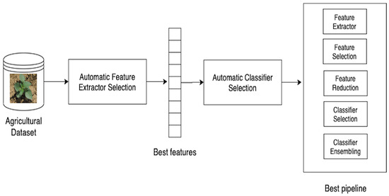
In this paper, a methodology integrating two AutoML steps was evaluated. As in [20], the assumption was that this combination with the correct configuration could obtain similar performances when compared to more traditional approaches, such as a Softmax classifier on the top of a neural-based feature extractor. As shown in Figure 1, the first step in the methodology was used for finding the best performing feature extractor able to extract the most meaningful features from the images. This process was done by a Bayesian neural architecture search approach. The result of this first step was a deep neural network composed of several convolutional layers automatically fine-tuned. This neural network was responsible for extracting the best features from the original images. Once the features were extracted, the second step took place for finding a complete machine-learning-based pipeline that could obtain the best final performance. Inside this pipeline, algorithms for (i) feature selection, (ii) dimension reduction, and (iii) classification were tested. Specifically, the following techniques have been evaluated:

• Principal Component Analysis [21]: It is used for linear dimensionality reduction using Singular Value Decomposition (SVD) of the data to project it to a lower-dimensional space; and thus, the chances for overfitting can be reduced. Contrary to other dimensionality reduction methods, the input features are centered but not scaled before applying the SVD.
• Truncated Value Decomposition [22]: As the previous method, it was also used for dimensional reduction and, thus, to reduce overfitting. The main difference is that this method does not center de data before computing the SVD.
• Kernel Principal Component Analysis [23]: Similar to the first method, but it uses a non-linear dimensionality reduction by using kernels. Its objective is the same, remove feature redundancy for improving the generalization ability of the classifier.
• Univariate feature Selection: Used for feature selection, this method selects the best features based on univariate statistical tests. In this work, we have used the chi-squared, ANOVA F-value [24] and the mutual information techniques [25].
• Decision Tree: Used as a single classifier or part of the ensemble, this method uses a non-parametric learning method. Its advantage is that ideally it can be visualized in order to better understand why the classifier made a specific decision. However, if the tree is very complex, interpretation can be hard. Moreover, this method is prone to overfitting, which can be an important disadvantage in case the extracted features contain noise. To avoid this problem different ensembles have been tried: AdaBoosting, Extra Trees and Random Forests.
• AdaBoosting [26]: Used as a single classifier or part of the ensemble; it uses an ensemble-learning approach known as boosting where a decision tree is retrained several times putting more emphasis on those samples where the prediction is not accurate.
• Random Forests [27]: Used as a single classifier or part of the ensemble; this classifier is made up of a collection of decision trees, which have been trained on different data samples drawn from the input features, with a technique called bootstrap sampling. As a result, random forests could lead to low overfitting.
• Extra Trees [28]: Used as a single classifier or part of the ensemble; this method is very similar to the random forests, however, it does not use bootstrap sampling. This approach could increase the overfitting because bootstrapping makes it more diversified. Another difference is that it uses a random cut for node creation inside the tree, which could lead to a reduction in overfitting.

The classification part will be studied in this work, evaluating whether the use of classifier ensembles instead of a single one can improve the performance or at least reduce the variance in the results. The ensemble method will use a majority vote approach, where the category with a greater number of votes from the individual classifiers will be used as the final predicted category. The selection of this pipeline was automatically performed by using Bayesian optimization.

Since open-source solutions were used for building this methodology, the final resulting pipeline can be exported and deployed into an autonomous weed control system with either a standalone or a cloud-based solution, depending on latency and computational constraints.

2.2. Experimental Decisions

Although AutoML can run without any specific configuration, to extract knowledge of this process and learn its drawbacks and strengths, some experimental constraints have been set. This means that some AutoML pipeline configurations (i.e., the hyperparameter configuration) were set as constants during the evaluation of the methodology.

Table 2. Hyperparameters that are not modified during the experiments.

Hyperparameter Constants	Value
Max. trials per deep model	35
Epochs	100
Use of geometrical data augmentation	Yes
Image Size	64 × 64
Batch Size	8
Max. time per model fitting	2 min
Total time finding best classifier	20 min

shows the most important ones, which were selected based on some preliminary experiments showing suitable performances, and the availability of enough computational resources. In order to find the best feature extractor, the Bayesian optimization algorithm ran a maximum of 35 times. Each deep model used a maximum of 100 epochs with a batch size of eight for model training. Regarding the classifier ensemble part, a maximum of 2 min was set for training every model of the ensemble; and 20 min for training all of them. The feature extractor used several data augmentation techniques before trying to extract the features. Among them, images could be horizontally rotated, cropped, scaled, or mirrored. Moreover, all the images were resized to 64 × 64 pixels and, therefore, the correlation between image size and physical size of the plants was removed, improving the generalization ability of the AutoML system.

On the other hand, other architectural configurations were empirically evaluated to find the most suitable one. This process was used for validating the robustness of some hyperparameters (shown in

Table 3. Hyperparameters evaluated to find the most suitable AutoML pipeline configuration.

Hyperparameter Variables	Value
Plant Segmentation	{Yes, No}
Noisy training	{Yes, No}
Use of fully-connected network	{Yes, No}
Classifier type	{Softmax, Single, Ensemble}

) against other modifications in the AutoML pipeline design. The presence of the background in the image could have an important impact when extracting features, and the use of plant segmentation (or not) has been evaluated. The segmentation has been implemented using a thresholding method on the Hue-Saturation-Value (HSV) color space. Since the high robustness of any automatic weeds identifier system is critical, the use of noisy samples in the training phase for improving the performance was also evaluated. Another important factor for training the feature extractor was whether to use a fully-connected network between the convolutional layers and the Softmax classifier. Both options were evaluated. Finally, once the features were extracted, a Softmax classifier, a single classifier, or an ensemble of classifiers could be used for classifying the input image. All these options were evaluated.

2.3. Datasets Used

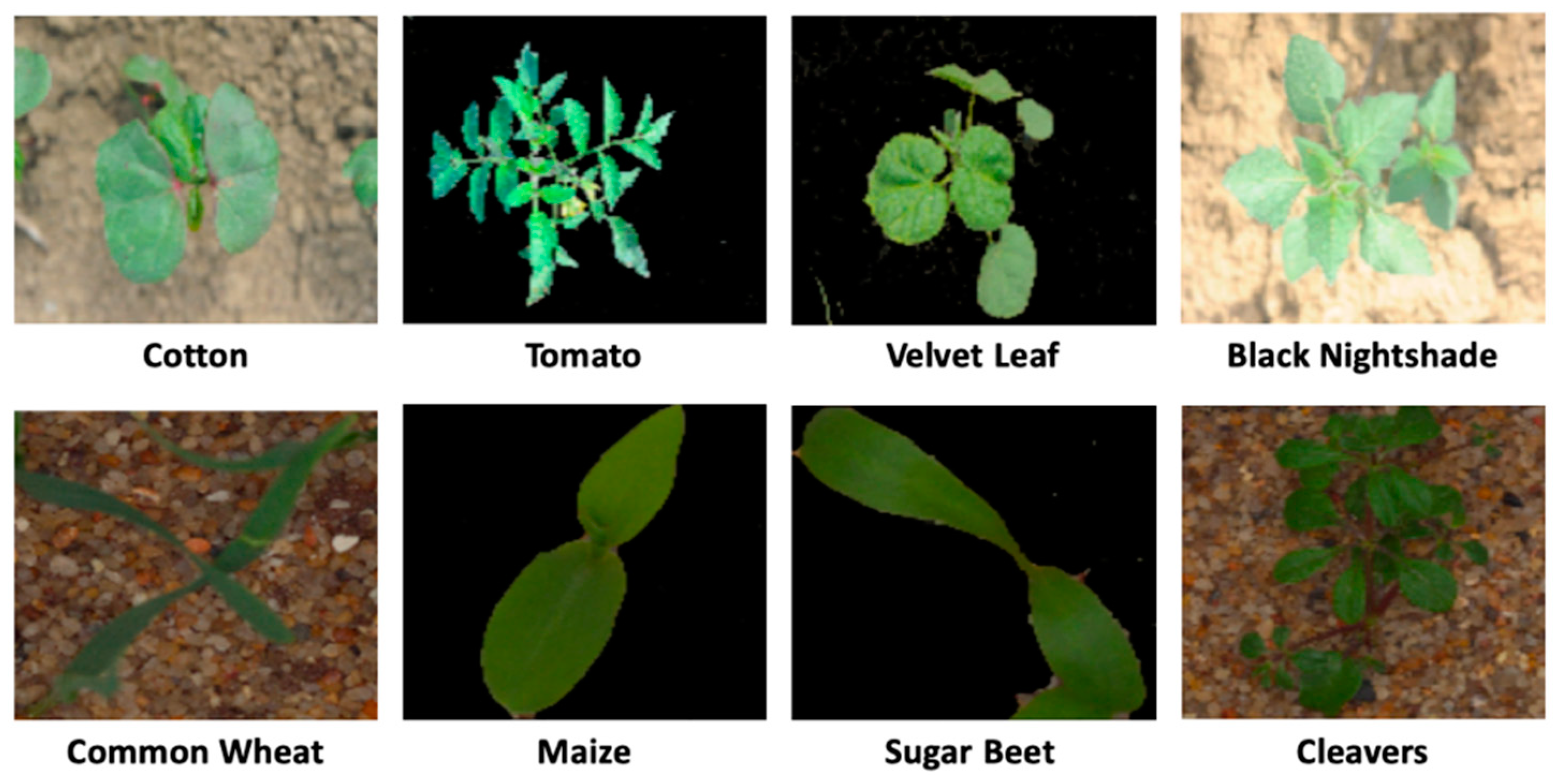
Two main datasets were used in this work: (i) The Early Crop Weeds dataset and (ii) the Plant Seedlings dataset. The first one contained 504 RGB images of four species at early growth stages. This dataset was collected by ourselves and presented in our previous research [10]. The second one contained RGB images of approximately 960 unique plants belonging to 12 species at several growth stages, with a physical resolution of roughly 10 pixels per mm. More information about this dataset can be found in [29]. Figure 2 shows several instances of the images available in both datasets; some of them after plant segmentation application. As it can be observed, the illumination conditions are rather variable in the first dataset, which will show the ability of the AutoML system for generalizing and setting the brightness of the picture as an irrelevant factor for crop/weeds identification. Regarding the second dataset, the images were taken from plants that were grown indoors in a greenhouse with artificial light to supplement natural light. This means that data were recorded under laboratory conditions and some aspects and morphological features of outdoor-grown plants are not present.

2.4. Evaluation

The performance of the AutoML system was measured with the F₁ score (Equation (1)). This metric is widely used for evaluating classification tasks, where recall is the ratio of the correct categories regarding the original dataset, and precision is the ratio of correct labels in the classifier output [30]. Since we addressed a multi-class problem in both datasets, it was necessary to compute the micro-averaged F₁ score for comparison purposes. This kind of aggregation is preferable over the macro-average when there is a class imbalance, as in the case of both datasets used in this work. On the other hand, for statistical comparisons, Friedman test [31] and Wilcoxon signed-rank test [32] were used. Both of them are paired non-parametric statistical tests, making them more robust to avoid too optimistic conclusions. The first one was used for testing equivalent performances among sets of two or more pipelines. The second one was used for testing equivalent performances among the same pipelines on two different datasets (i.e., clean and noisy datasets)

$${\mathrm{F}}_{1}score=\frac{2\times precision\times recall}{precision+recall}$$

(1)

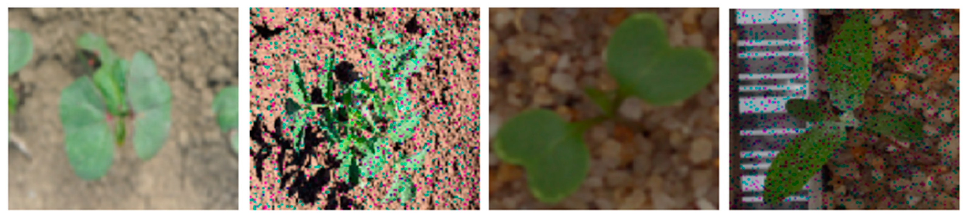
Since AutoML could easily lead to overfitting, the difference between the F₁ score on the train and test datasets was also measured as an important metric to take into account. This way, it was possible to also know whether the AutoML pipeline found a classifier that was able to generalize for recognizing new weed examples or it has just fit training data, and therefore, it could not be applied in a real-world situation. Moreover, this evaluation of the robustness has been studied under harder situations: blurry and salt and pepper noisy images [33]. The micro-averaged F₁ score has also been measured with fully noisy datasets as shown in Figure 3. The explanation and consequences of this robustness problem of deep learning-based systems were widely explained in [12].

2.5. Hardware and Software

Two main software packages were used in this work: AutoKeras 1.0.8 and Auto-Sklearn 0.10.0. The first one optimizes both architecture and hyperparameters using neural network morphism guided by Bayesian optimization to select the most promising operations at each stage. It uses Tensorflow 2.3.8 and Keras 2.4.3 [34] backends. The second one, Auto-Sklearn, is an open-source library for performing AutoML with non-deep learning algorithms. It makes use of Scikit-Learn machine learning library (version 0.22.2) for data transformations and machine learning. Like AutoKeras, it also uses a Bayesian Optimization search procedure to efficiently discover a top-performing model pipeline for a given set of features. As the image preprocessing library, OpenCV 3.4.2 was used. All the experiments were run on Ubuntu 18.04 as the OS, and a GeForce RTX 2080Ti GPU.

3. Results

In this section, the results for finding the best AutoML pipeline on every dataset are presented. To reduce the volatility of the experiments, each pipeline configuration was evaluated 10 times under different random seeds, and results reported the mean of the F₁ score for each configuration on every dataset (clean/original and noisy ones). Regarding data splitting, a stratified split was performed with 50% of the samples used for training, 25% for validation, and 25% for testing. Additionally, when a noisy version of a dataset is mentioned, that means that noise was added on the 50% of the dataset samples used for training (25% salt and pepper and 25%). Finally, it is important to remark that the “Overfitting” column reports the difference between the performance in the training set and the performance in the test set. The latter one is shown in the “F₁ Score” column.

3.1. Early Crop Weeds Dataset

3.1.1. Training on the Original Dataset

Table 4. Top 10 best AutoML configurations in the Early Crop Weeds Dataset (mean ± standard deviation). (PS: Plant Segmentation; FC: Fully-Connected).

PS	FC	Classifier	F1 Score	Overfitting	Salt F1	Blur F1
Yes	No	Ensemble	93.7 ± 1.13	6.28 ± 1.06	90.93 ± 5.56	69.07 ± 11.54
Yes	No	Single	93.6 ± 1.6	6.4 ± 1.6	88.4 ± 6	70.8 ± 2
No	Yes	Ensemble	92.15 ± 2.4	7.82 ± 2.58	60.8 ± 8	49.2 ± 14.8
Yes	No	Softmax	91.9 ± 6.36	7.84 ± 6.67	87.2 ± 9.24	67.6 ± 9.81
Yes	Yes	Softmax	91.89 ± 2.24	5.93 ± 2.69	89.26 ± 4.7	63.89 ± 11.89
Yes	Yes	Single	91.84 ± 2.45	8.09 ± 2.48	90.24 ± 3.09	62.88 ± 10.76
Yes	Yes	Ensemble	91.31 ± 2.94	8.58 ± 3.01	88.8 ± 3.42	62.63 ± 10.8
No	Yes	Single	90.4 ± 1.6	9.42 ± 1.78	64 ± 4.8	52.4 ± 12.4
No	No	Ensemble	86 ± 4.4	12.93 ± 3.33	62.8 ± 5.2	49.2 ± 7.6
No	Yes	Softmax	85.6 ± 1.6	7.64 ± 3.03	52 ± 9.6	52 ± 20.8

presents a ranking of the 10 best AutoML pipelines in terms of F₁ score regarding the Early Crop Weeds dataset. After running the Friedman test with a confidence level of 0.1, the first four pipelines could be considered equivalent. Inside this set, the use of plant segmentation and not using a fully-connected network can lead to better performances in comparison to other combinations. It could be discussed that by integrating the classifiers into the analysis, the Softmax had a greater variance in the results and thus, its robustness could be a problem. In fact, this pipeline could be considered to be out of the previous set if we reduce the confidence level to 0.06. On the other hand, out of this set, it can be found that the combination at the same time of plant segmentation and a fully-connected network showed a lower performance. Observing the “Overfitting” column, it can be noticed that some pipelines obtained performances close to 100% on the training set. For instance, if the system appearing in the first row is selected, the performance on the training set was 99.98% on average (93.7% + 6.28%). Table 4 also shows the performance of the systems when a noisy test dataset was used for evaluation. As it can be observed, performance decreased in most of the cases (Wilcoxon p-value < 0.01) with both types of noises (salt and pepper and blurring), although, according to the results, the blurry images were harder to classify accurately. It is important to note that there were some systems that maintained a good performance for salt and pepper noise (see rows 1, 2, 4 and 5), but in the case of the system that did not use plant segmentation, used a fully-connected network and a classifier ensemble on the top (row 3), the performance decreased a 34.02% for salt and pepper noise and 46.61% for blurring, which shows a clear lack of robustness against these types of noise.

3.1.2. Training on a Noisy Version of the Dataset

Table 5. Top 10 best AutoML configurations in the Plant Seedlings Dataset (mean ± standard deviation). (PS: Plant Segmentation; FC: Fully-Connected).

PS	FC	Classifier	F1 Score	Overfitting	Salt F1	Blur F1
Yes	Yes	Ensemble	93.8 ± 3.44	6.09 ± 3.4	93 ± 4.41	93.4 ± 4.25
Yes	Yes	Single	92.91 ± 4.71	6.93 ± 4.64	92.57 ± 4.87	92.11 ± 4.37
Yes	Yes	Softmax	92.09 ± 4.73	7.46 ± 4.86	92.27 ± 4.8	90.84 ± 4.65
No	No	Single	91.6 ± 4.88	8.04 ± 4.96	88 ± 4.38	90.2 ± 5.7
Yes	No	Softmax	91.04 ± 2.84	8.5 ± 3.13	90.72 ± 2.89	90.4 ± 2.21
No	No	Ensemble	90.4 ± 5.84	9.39 ± 5.83	85.28 ± 7	89.28 ± 5.53
Yes	No	Single	88 ± 2.36	11.82 ± 2.5	88.53 ± 3.02	89.6 ± 2.85
Yes	No	Ensemble	88.8 ± 1.96	11.02 ± 2.1	88.8 ± 2.85	89.17 ± 3.22
No	No	Softmax	87.73 ± 6.95	11.67 ± 7.21	80 ± 10.28	87.07 ± 5.72
No	Yes	Softmax	87.47 ± 8.17	11.76 ± 8.53	86.4 ± 7.92	86.4 ± 10.2

shows how the AutoML pipelines improved (or not), when they were trained using noisy samples in part of the training dataset (50% clean, 25% salt and pepper, and 25% blurring). After running the Friedman test with a confidence level of 0.1, the first four pipelines could be considered as having equivalent performances (“F₁ score” column), but overcoming the rest of the pipelines. In this set of pipelines, it could be found that the combination of plant segmentation and a fully-connected classifier could lead to superior performances under noisy conditions. This contrasted with the findings remarked in Table 4, where this combination was not among the best systems. Regarding the results shown in the “F₁ score” column, the performances were highly aligned with the ones presented in Table 4. This means that training the AutoML systems with noisy data could lead to pipelines with similar performances to fully-clean datasets. However, the variance and the performance of specific pipelines could decrease. For example, there were some top-performers systems in Table 4 that reduced their performances under the noisy configuration. For instance, the system presented in the first row of Table 4, decreased its performance by 5.23% (from 93.7% to 88.8%) on the clean test set and by 2.34% (from 90.93% to 88.8%) on the salt and pepper noisy test set (see Table 5; row 8). However, its performance improved on the blurry dataset (from 69.07% to 89.17%). This means that using noisy samples during training could lead some systems to perform better on a clean dataset (see Table 4; row 7 and Table 5; row 1), but also to decrease it (see Table 4; row 1 and Table 5; row 8). The most prominent differences could be found in the evaluation with blurry datasets, where performances significantly increased (Wilcoxon p-value < 0.05) in all cases.

3.2. Plant Seedlings Dataset

3.2.1. Training on the Original Dataset

Table 6. Top 10 best AutoML configurations in the Plant Seedlings Dataset (Mean ± standard deviation). (PS: Plant Segmentation; FC: Fully-Connected).

PS	FC	Classifier	F1 Score	Overfitting	Salt F1	Blur F1
Yes	No	Ensemble	90.74 ± 0.8	8.51 ± 1.25	72.89 ± 7.52	72.06 ± 17.83
Yes	No	Single	90.16 ± 0.67	9.3 ± 0.83	75.43 ± 1.22	80.94 ± 3.65
Yes	Yes	Single	88.64 ± 0.66	11.04 ± 0.42	80.96 ± 1.56	86.62 ± 1.09
No	No	Ensemble	88.63 ± 1.26	8.16 ± 0.3	60.94 ± 17.33	83.57 ± 0.83
Yes	Yes	Ensemble	88.5 ± 1.44	11.01 ± 1.64	81.25 ± 1.89	86.11 ± 1.39
No	No	Single	88.23 ± 1.08	8.89 ± 0.67	58.81 ± 19.24	83.21 ± 0.61
Yes	Yes	Softmax	87.44 ± 1.36	5.56 ± 1.99	81.06 ± 1.43	85.78 ± 1.75
Yes	No	Softmax	87.17 ± 2.63	6.37 ± 1.02	67.74 ± 6.18	71.59 ± 17.24
No	Yes	Single	86.84 ± 0.76	12.08 ± 1.59	60.49 ± 8.7	83.21 ± 2.23
No	Yes	Ensemble	86.43 ± 1.14	13.08 ± 1.6	62.82 ± 7.54	82.42 ± 2.61

presents a ranking of the 10 AutoML pipelines showing the highest performance in terms of F₁ score regarding the Plant Seedlings dataset. After running the Friedman test with a confidence level of 0.01, the first two rows show the pipelines with the best performances (F₁ score column). These configurations had in common the use of plant segmentation and avoiding a fully-connected network for feature extraction. Regarding the classifier part, the replacement of Softmax by a new classifier (both ensemble and single) reported the best performances (90.74 ± 0.8 and 90.16 ± 0.67 respectively). These results were aligned with the findings presented in Table 4. Thus, it could be discussed that these configurations worked well across datasets, which did not present noise and could be a good baseline for future experiments. Among the hyper-parameters, plant segmentation was again a good option for obtaining the best results. Removing the Softmax classifier and training an extra classifier on the top of the feature extractor seemed to have a general good behavior: 8 of the 10 best systems used this technique. Finally, as it happened with the Early Crop Weeds dataset, all the systems drastically reduced their performance when they were evaluated on noisy datasets (Wilcoxon p-value < 0.01). However, it is important to note that these reductions were not equal. Some systems were more robust to a specific type of noise (see Table 6; row 4), and others reduced their performance but less than the general behavior (see Table 6; row 7). Observing the “Overfitting” column, in general, higher values than the reported in Table 4 can be found. For instance, this could be the case of the first two pipelines in both tables (Wilcoxon p-value < 0.01).

3.2.2. Training on a Noisy Version of the Dataset

Table 7. Top 10 best AutoML configurations in the Plant Seedlings Dataset (Mean ± standard deviation). (PS: Plant Segmentation; FC: Fully-Connected).

PS	FC	Classifier	F1 Score	Overfitting	Salt F1	Blur F1
Yes	Yes	Softmax	86.98 ± 1.92	12.26 ± 2.15	84.55 ± 1.79	87.34 ± 2.11
Yes	No	Ensemble	85.97 ± 4.24	13.88 ± 4.07	85.01 ± 3.91	85.87 ± 4.51
Yes	No	Single	85.29 ± 5.29	14.4 ± 4.9	84.28 ± 4.51	84.81 ± 5.03
No	No	Ensemble	83.78 ± 3.9	15.49 ± 4.42	81.76 ± 3.25	83.13 ± 3.86
Yes	No	Softmax	83.63 ± 5.74	15.87 ± 5.84	82.31 ± 4.67	83.06 ± 5.91
No	Yes	Softmax	83.59 ± 4.17	13.6 ± 6.73	81.48 ± 3.78	83.19 ± 3.45
No	No	Single	83.37 ± 3.77	15.46 ± 4.56	81.11 ± 3.17	82.86 ± 3.21
No	No	Softmax	80.45 ± 4.13	17.61 ± 6.94	78.72 ± 3.22	80.09 ± 4
No	Yes	Ensemble	65.31 ± 30.4	12.57 ± 7.74	63.74 ± 29.54	65.52 ± 30.56
No	Yes	Single	65.09 ± 30.44	12.25 ± 8.08	63.03 ± 29.28	64.93 ± 30.32

shows how the AutoML pipelines improved (or not) when they were trained using noisy samples (50% clean, 25% salt and pepper, and 25% blurring). After running the Friedman test with a confidence level of 0.05, the first four rows show the pipelines with the best performances. The most repeated hyper-parameters in these systems were the use of plant segmentation and not using a fully-connected network. As it was expected, a general improvement is observed in the evaluation with noisy datasets. However, as it was also observed in Table 5, the “Overfitting” column reports overall worse results (Wilcoxon p-value < 0.1). This could mean that the pipelines were not able to generalize correctly.

3.3. Visual Analysis of Experimental Variables

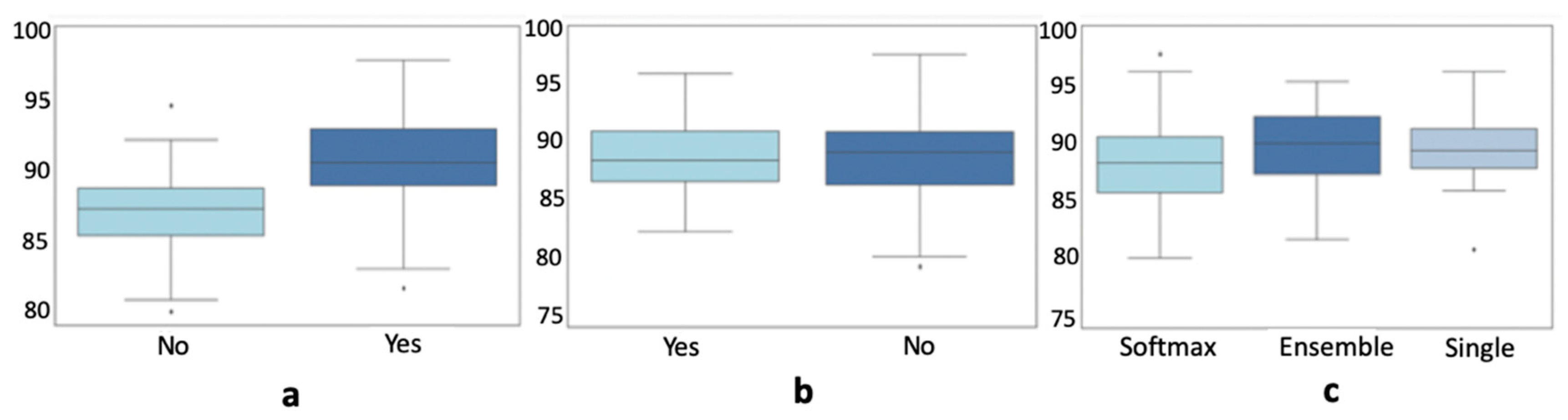
From the analysis of the results presented in previous sections, it has been observed that some hyper-parameters altered more the final performances. Figure 4a, which integrates the results obtained in both datasets, confirms that the use of plant segmentation as a pre-processing technique led to better performance. This neural network was responsible for extracting the best features from the original images. Once the features were extracted, the second step took place for finding a complete machine-learning-based pipeline that could obtain the best final Figure 4b). The same happened with the type of classifier. Figure 4c shows that the classifier with the best median was the ensemble approach, but single and Softmax classifiers could also obtain good performances. In the case of the single classifier, the variance was lower than the Softmax approach, pointing to it as a more robust classifier. After running the Wilcoxon test for comparing the different distributions, only the use of plant segmentation presented a significant difference in relation to its alternative (p-value < 0.01).

4. Discussion

The results have shown that AutoML can provide classifiers with performances over 90% F₁ score. These results were aligned with other related works [20,35,36] but they were lower than our previous work concerning performance [37]. However, the disadvantage of our previous work was that obtaining better results took significantly longer for fine-tuning precise nuances of deep neural networks by experts on deep learning, and this process could be avoided or shortened by using AutoML. The main effort of the current work was dedicated to creating a reliable experimental setup for evaluating AutoML performance under different conditions, but not for finding suitable ML pipelines, which was done automatically by the Bayesian optimization of the AutoML frameworks. Moreover, it is important to remark that the pipelines evaluated in this work were constrained in some resources (see Table 2); which means that with more time or trials for finding the correct configuration, the results could improve in both F₁ score and for robustness against overfitting. Since AutoML works and speeds up many tasks, finding a good balance between manual expert machine learning tuning, AutoML and good performances will be a future open topic for research and discussion.

One of the research questions this work tried to answer was whether integrating an AutoML process on top of a deep neural-based feature extractor could increase the performance over a Softmax classifier. According to the results, it is difficult to provide a final answer. Depending on the dataset and the existence (or not) of noise, different patterns can be observed. According to Figure 4c, the Softmax classifier was able to obtain the highest performances but it was more unstable; the use of a replacement with a single classifier reported a higher median, lower variance, but it did not reach the highest performance. The ensemble approach obtained an intermediate response having the highest median but higher variance than the single classifier approach. As a conclusion, it could be stated that all these possibilities should be evaluated until new research works enlighten more specific results. Finally, from the different configurations evaluated, only the use of plant segmentation reported repeatedly better performances.

Related to the previous research question, it could be discussed whether there was a relevant pattern in the machine learning pipelines on the top of the neural-based feature extraction. According to the results, the Bayesian optimization has followed different paths leading to different combinations of feature selection, dimensional reduction and classifier tuning. This could mean that a slight difference in the dataset could produce a completely different pipeline, where, for instance, the classifier could be either a decision tree or a random forest without any of them overcoming the other option. This is highly related to the no-free-lunch theorem [38], which could be even more noticeable within AutoML. Additionally, although tree ensembles have been used to avoid overfitting, the results shown in the tables presented some overfitting, which will reduce the applications where these systems could run safely. It could be concluded that AutoML adds a new complexity layer, where a compromise between interpretability and performances should be established according to the final application and its risks.

Another addressed question was whether the evaluation on a noisy dataset would reduce the performance of systems working accurately on a clean dataset. As Table 4 and Table 6 show, the answer has been positive. All systems have reduced their performances when trying to classify images that contain noise. This behavior shows the inability to adapt to possible problems that can occur in the field. On the other hand, these noisy images would be easily classified by a human being, and therefore, it would be necessary to find a way to overcome this limitation. The solution evaluated in this paper has been to use noisy samples during training. However, according to Table 5 and Table 7, the responses of every pipeline were quite different. There were pipelines that improved in both clean and noisy datasets, while there were other pipelines that reduced their performance in some cases. It could be discussed that depending on the risks and the types of noises that the weeds identification system could suffer, one approach or another should be implemented.

One of the research decisions made during this work was to implement a solution based on open-source technologies. Although the use of some closed cloud-based solutions such as Google Vision can work as a final solution ready for being deployed in production, having access to the whole code and workflow of the solution is desired for advancing machine learning research in general and the AutoML techniques in specific. Due to the novelty of this research area, understanding the factors and parameters which potentially could lead to a better solution, is important. The results shown along with this paper could provide insights about which hyper-parameters should be studied in the future. For instance, batch size (8) and image size (64 × 64) were set as experimental constants, but increasing them could lead to new relevant results in the domain of precision agriculture. After the fine-tuning effort, once an open suitable AutoML pipeline has been found and reported, it could make sense to share the pipeline through a cloud-based solution (not necessarily closed), which could expose the functionality of predicting new samples, and which could be accessed by automatic control weed systems. In summary, closed cloud-based solutions would make more sense being used in the context of operational applications.

Finally, it can be concluded that AutoML could help the agrotechnology community to easily test machine-learning-based solutions requiring fewer resources to be invested in the implementation part of the solution and dedicating more resources to the domain part of the problem. Moreover, due to the dynamic nature of agriculture, the AutoML pipeline presented in this work could easily create a new model based on new samples, speeding up the deployment of high-performing solutions.

5. Conclusions

In this work, a weeds identification system methodology was evaluated by using an integration of two different AutoML systems. Moreover, two different datasets containing 4 and 13 classes of crops, seedlings, and weeds have been used as benchmarks. The best-evaluated systems under the proposed methodology have shown promising performances between 90% and 93% F₁ score depending on the dataset and the existence (or not) of noisy samples. Although results were aligned to previous AutoML works, the implementation of more resource exhaustive practices, such as increasing the batch size while training, will be examined in the future. Moreover, using new datasets, such as the DeepWeeds dataset (https://github.com/AlexOlsen/DeepWeeds (accessed on 8 February 2021)), will provide more insights about the real generalization ability of the AutoML technology. Additionally, experiments using noisy samples for testing the robustness of the systems will be extended. On the one hand, smearing noise will be used due to its relation with the movement of the vehicles, which could lead to new insights into the implementation of autonomous vehicles used in precision agriculture. On the other hand, training by using one type of noise and evaluating on a test set with a different type of noise will be checked in order to discern any relation among the different types of noise. Finally, since the use of ensembles of decision trees has not avoided a certain degree of overfitting, new machine learning pipelines will be studied. On the one hand, increasing the number of decision trees inside the ensemble will be evaluated; on the other, a new ensemble technique will be studied: the Super Learner [39], a model stacking method, where a classifier trains on the top of the predictions provided by the individual trained models. For validating its performance, a more sophisticated approach will be used. Every classifier type will be studied separately, constraining the Bayesian search to a smaller subset, which could lead to a better understandability of the obtained results.

References

- European Crop Protection (ECPA). With or Without Pesticides? 2017. Available online: https://croplifeeurope.eu/ (accessed on 1 October 2020).
- European Parliamentary Research Service (EPRS). Farming without Plant Protection Products: Can We Grow without Using Herbicides, Fungicides and Insecticides? Scientific Foresight Unit (STOA): Brussels, Belgium, 2019. [Google Scholar]
- European Commision. A Farm to Fork Stragegy for a Fair, Healthy and Environmentally-Friendly Foods System. Communication from the Commision to the European Parlianment, the Council, the European Economic and Social Committee and the Committee of the Regions. Available online: https://ec.europa.eu/food/farm2fork_en (accessed on 28 January 2020).
- Gonzalez-de-Santos, P.; Ribeiro, A.; Fernández-Quintanilla, C.; López-Granados, F.; Brandstötter, M.; Tomic, S.; Pedrazzi, S.; Peruzzi, A.; Pajares, G.; Kaplanis, G.; et al. Fleets of robots for environmentally-safe pest control in agriculture. Precis. Agric. 2016, 18, 574–614. [Google Scholar] [CrossRef]
- Van Evert, F.K.; Fountas, S.; Jakovetic, D.; Crnojevic, V.; Travlos, I.; Kempenaar, C. Big Data for weed control and crop protection. Weed Res. 2017, 57, 218–233. [Google Scholar] [CrossRef] [Green Version]
- Fernández-Quintanilla, C.; Peña, J.M.; Andújar, D.; Dorado, J.; Ribeiro, A.; López-Granados, F. Is the current state of the art of weed monitoring suitable for site-specific weed management in arable crops? Weed Res. 2018, 58, 259–272. [Google Scholar] [CrossRef]
- Potena, C.; Nardi, D.; Pretto, A. Fast and accurate crop and weed identification with summarized train sets for precision agriculture. Adv. Intell. Syst. Comput. 2016, 531, 105–121. [Google Scholar]
- Mohanty, S.P.; Hughes, D.P.; Salathé, M. Using Deep Learning for Image-Based Plant Disease Detection. Front. Plant Sci. 2016, 7, 1419. [Google Scholar] [CrossRef] [Green Version]
- Sladojevic, S.; Arsenovic, M.; Anderla, A.; Culibrk, D.; Stefanovic, D. Deep Neural Networks Based Recognition of Plant Diseases by Leaf Image Classification. Comput. Intell. Neurosci. 2016, 2016, 3289801. [Google Scholar] [CrossRef] [PubMed] [Green Version]
- Espejo-García, B.; Mylonas, N.; Athanasakos, L.; Fountas, S.; Vasilakoglou, I. Towards weeds identification assistance through transfer learning. Comput. Electron. Agric. 2020, 171, 105306. [Google Scholar] [CrossRef]
- Olsen, A.; Konovalov, D.A.; Philippa, B.; Ridd, P.; Wood, J.C.; Johns, J.; Banks, W.; Girgenti, B.; Kenny, O.; Whinney, J.; et al. DeepWeeds: A Multiclass Weed Species Image Dataset for Deep Learning. Sci. Rep. 2019, 9, 1–2. [Google Scholar] [CrossRef]
- Barbedo, J.G.A. Factors influencing the use of deep learning for plant disease recognition. Biosyst. Eng. 2018, 172, 84–91. [Google Scholar] [CrossRef]
- Feurer, M.; Klein, A.; Eggensperger, K.; Springenberg, J.; Blum, M.; Hutter, F. Efficient and robust automated machine learning. Adv. Neural. Inf. Process. Syst. 2015, 28, 2962–2970. [Google Scholar]
- Kotthoff, L.; Thornton, C.; Hoos, H.H.; Hutter, F.; Leyton-Brown, K. Auto-WEKA 2.0: Automatic model selection and hyperparameter optimization in WEKA. J. Mach. Learn. Res. 2017, 18, 826–830. [Google Scholar]
- Hayashi, M.; Tamai, K.; Owashi, Y.; Miura, K. Automated machine learning for identification of pest aphid species (Hemiptera: Aphididae). Appl. Entomol. Zool. 2019, 54, 487–490. [Google Scholar] [CrossRef]
- Montellano, J.M. Butterfly, Larvae and Pupae Defects Detection Using Convolutional Neural Network and Apriori Algorithm; Springer: Cham, Switzerland, 2019. [Google Scholar]
- Hsieh, J.Y.; Huang, W.; Yang, H.T.; Lin, C.C.; Fan, Y.C.; Chen, H. Building the Rice Blast Disease Prediction Model Based on Machine Learning and Neural Networks; EasyChair: Manchester, UK, 2019. [Google Scholar]
- Kiala, Z.; Mutanga, O.; Odindi, J.; Peerbhay, K.Y.; Slotow, R. Automated classification of a tropical landscape infested by Parthenium weed (Parthenium hyterophorus). J. Remote Sens. 2020, 41, 8497–8519. [Google Scholar] [CrossRef]
- Koh, J.C.; Spangenberg, G.; Kant, S. Automated Machine Learning for High-Throughput Image-Based Plant Phenotyping. bioRxiv 2020. [Google Scholar] [CrossRef]
- Suh, H.K.; IJsselmuiden, J.; Hofstee, J.; Henten, E.V. Transfer learning for the classification of sugar beet and volunteer potato under field conditions. Biosyst. Eng. 2018, 174, 50–65. [Google Scholar] [CrossRef]
- Tipping, M.E.; Bishop, C.M. Probabilistic Principal Component Analysis. Neural Comput. 1999, 11, 443–482. [Google Scholar] [CrossRef] [PubMed]
- Halko, N.; Martinsson, P.; Tropp, J. Finding Structure with Randomness: Probabilistic Algorithms for Constructing Approximate Matrix Decompositions. Siam Rev. 2011, 53, 217–288. [Google Scholar] [CrossRef]
- Schoelkopf, B.; Smola, A.; Mueller, K.-R. Kernel principal component analysis. In Advances in Kernel Methods; MIT Press: Cambridge, MA, USA, 1999; pp. 327–352. [Google Scholar]
- Agresti, A. An Introduction to Categorical Data Analysis, 3rd ed.; John Wiley & Sons: Hoboken, NJ, USA, 2018. [Google Scholar]
- Ross, B.C. Mutual Information between Discrete and Continuous Data Sets. PLoS ONE 2014, 9, e87357. [Google Scholar] [CrossRef]
- Freund, Y.; Schapire, R. A decision-theoretic generalization of on-line learning and an application to boosting. J. Comput. Syst. 1995, 55, 119–139. [Google Scholar] [CrossRef] [Green Version]
- Breiman, L. Random Forests. Mach. Learn. 2004, 45, 5–32. [Google Scholar] [CrossRef] [Green Version]
- Geurts, P.; Ernst, D.; Wehenkel, L. Extremely randomized trees. Mach. Learn. 2006, 63, 3–42. [Google Scholar] [CrossRef] [Green Version]
- Giselsson, T.M.; Dyrmann, M.; Jørgensen, R.N.; Jensen, P.K.; Midtiby, H.S. A Public Image Database for Benchmark of Plant Seedling Classification Algorithms. Arxiv Prepr. 2017, arXiv:1711.05458. [Google Scholar]
- Manning, C.D.; Raghavan, P.; Schütze, H. Introduction to Information Retrieval; University Press: Cambridge, UK, 2008. [Google Scholar]
- Friedman, M. The Use of Ranks to Avoid the Assumption of Normality Implicit in the Analysis of Variance. J. Am. Stat. Assoc. 1937, 32, 675–701. [Google Scholar] [CrossRef]
- Ramachandran, K.; Tsokos, C.P. Mathematical Statistics with Applications; Elsevier: Berkeley, CA, USA, 2009. [Google Scholar]
- Fu, B.; Zhao, X.; Ren, Y.; Li, X.; Wang, X. A salt and pepper noise image denoising method based on the generative classification. Multimed. Tools Appl. 2018, 78, 12043–12053. [Google Scholar] [CrossRef] [Green Version]
- Chollet, F. Keras. 2015. Available online: https://keras.io (accessed on 5 January 2021).
- Christiansen, P.; Dyrmann, M. Automated Classification of Seedlings Using Computer Vision; Aarhus University: Aarhus, Denmark, 2014. [Google Scholar]
- Dyrmann, M.; Karstoft, H.; Midtiby, H. Plant species classification using deep convolutional neural network. Biosyst. Eng. 2016, 151, 72–80. [Google Scholar] [CrossRef]
- Espejo-García, B.; Mylonas, N.; Athanasakos, L.; Fountas, S. Improving weeds identification with a repository of agricultural pre-trained deep neural networks. Comput. Electron. Agric. 2020, 175, 105593. [Google Scholar] [CrossRef]
- Wolpert, D.; Macready, W. No free lunch theorems for optimization. IEEE Trans. Evol. Comput. 1997, 1, 67–82. [Google Scholar] [CrossRef] [Green Version]
- Laan, M.J.; Polley, E.; Hubbard, A. Super learner. Stat. Appl. Genet. Mol. Biol. 2007, 6, 25. [Google Scholar]
Figure 1.
Methodology evaluated for AutoML implementation covering (i) automatic feature extraction and (ii) automatic pipeline selection: feature selection + feature reduction + classification. Inside green boxes, we can find the components that (hypothetically) the Bayesian optimization would choose as the best ones.
Figure 2.
Image samples from the benchmark datasets. The first row shows pictures from the Early Crop Weeds Dataset; the second row shows pictures from the Plant Seedlings Dataset.
Figure 3.
Noisy samples from both datasets. From left to right: blurry cotton, tomato with salt and pepper noise, blurry charlock and fat hen with salt and pepper noise.
Figure 4.
Statistical Analysis of (a) plant segmentation; (b) Fully-Connected network use; (c) classifier type.