
Year-Independent Prediction of Food Insecurity Using Classical and Neural Network Machine Learning Methods


1
Data Analytics Certificate Program, Graduate School of Engineering and Management, Air Force Institute of Technology, Wright-Patterson AFB, Dayton, OH 45433, USA
2
The Perduco Group (a LinQuest Company), Dayton, OH 45433, USA
*
Author to whom correspondence should be addressed.
AI 2021, 2(2), 244-260; https://0-doi-org.brum.beds.ac.uk/10.3390/ai2020015
Submission received: 19 April 2021
/
Revised: 15 May 2021
/
Accepted: 19 May 2021
/
Published: 23 May 2021
Abstract
:Current food crisis predictions are developed by the Famine Early Warning System Network, but they fail to classify the majority of food crisis outbreaks with model metrics of recall (0.23), precision (0.42), and f1 (0.30). In this work, using a World Bank dataset, classical and neural network (NN) machine learning algorithms were developed to predict food crises in 21 countries. The best classical logistic regression algorithm achieved a high level of significance (p < 0.001) and precision (0.75) but was deficient in recall (0.20) and f1 (0.32). Of particular interest, the classical algorithm indicated that the vegetation index and the food price index were both positively correlated with food crises. A novel method for performing an iterative multidimensional hyperparameter search is presented, which resulted in significantly improved performance when applied to this dataset. Four iterations were conducted, which resulted in excellent 0.96 for metrics of precision, recall, and f1. Due to this strong performance, the food crisis year was removed from the dataset to prevent immediate extrapolation when used on future data, and the modeling process was repeated. The best “no year” model metrics remained strong, achieving ≥0.92 for recall, precision, and f1 while meeting a 10% f1 overfitting threshold on the test (0.84) and holdout (0.83) datasets. The year-agnostic neural network model represents a novel approach to classify food crises and outperforms current food crisis prediction efforts.
1. Introduction
The global Westphalian system, as described by Henry Kissinger, enshrines the basis of a global world order that recognizes the sovereignty of nation states and allows for the formation of a balance of power [1]. Through this framework, international trade and financial institutions arose and encouraged the development of principles to resolve conflict and “set limits on the conduct of war” [1]. In this system, according to the geopolitical analyst Robert Kaplan, it is in the interest of the United States (US) to ensure that there is no equally dominant power in the Eastern Hemisphere in order to protect treaties, de facto allies, and sea-based lines of communication [2]. Furthermore, the current National Defense Strategy calls for the United States to shift its focus from terrorism to strategic competition and to bolster the alliance network to shift the balance of power to its favor [3].
A potential challenge to the United States’ alliance network in the future is food scarcity as a nation experiencing a food crisis must focus inward instead of assisting other nations. Geopolitical analyst Zeihan notes that over three quarters of the world’s land is not hospitable to produce bedrock nutrition products such as wheat, rice, corn, and soy [4]. Zeihan also points out numerous examples of war motivated by food resources and that more governments have “collapsed throughout history from famine and failures in food distribution than by war, disease, revolution or terrorism” [4]. As the US is a net exporter of food, it has the ability to promote regional stability through food assistance. If the US can accurately predict when food crises will occur, it can most efficiently direct resources to those partners while increasing regional stability. Wischnath and Buhuag affirm Zeihan’s assertion using statistical analysis of food shortages and armed conflicts in India to demonstrate that a poor harvest is correlated with higher political violence [5]. Additionally, it is likely that climate change will result in increased future food crises, with higher transition rates of arable land to desert. The UN Intergovernmental Panel on Climate Change has established several greenhouse gas concentration scenarios, known as representative concentration pathway (RCP). Huang et al. indicates that if the worst-case scenario of RCP 8.5 is realized, “the area of moderate to very high desertification risk will increase by 23% by the end of this century” [6].
As a consequence of the destabilizing effects of food insecurity and the potential for it to be exasperated by a changing geographic landscape, it is imperative that governments and humanitarian organizations predict these features in advance. Current prediction efforts rely on a variety of demographic, geographic, and societal attributes but are not able to anticipate real-time shortfalls in crop production and landscape changes. To answer this, machine learning algorithms have recently been employed to predict crop yields, and remote sensing techniques are being evaluated to monitor drought and salinity stress simultaneously [7,8,9]. Thus, governments must continue to increase the fidelity with which they measure and respond to food insecurity.
In a World Bank working paper, Andree et al. used Famine Early Warning Systems Network (FEWS NET) data from 2007 to 2020 to predict food crises on three time horizons (4, 8, and 12 months in advance) using a random forest classifier [10]. The models were developed using a train and holdout data split, with the train set predicting crises from 2007 to 2019 and the holdout set predicting crises from 2019 to 2020. The results of the modeling effort were validated using 10-fold cross-validation on the training set at the district and national levels. The researchers processed the data using spatial and temporal lags, increased the food crisis indicator for districts receiving humanitarian assistance to net the effect of aid, and limited the number of pairwise covariates by the correlation coefficient (>0.75). In this work, the historical performance of FEWS NET district-level predictions for outbreaks of food crises from 2007 to 2019 were documented. The first model was a random forest without a penalty loss function, and the average performance for the validation set on time horizons 3–4 and 6–8 months in advance had poor precision (0.42), recall (0.23), and f1 (0.30) [10].
The final model in this work implemented a loss function that adjusted the penalties associated with false positives and false negatives. After implementing this loss function, the model achieved an average recall of 0.84 but at the expense of precision (0.36) and f1 (0.50) for district-level predictions 4 and 8 months in advance) [10]. However, the model performance on the holdout validation set (2019–2020) was degraded, possibly due to overfitting. For predictions 4 months in advance, the model’s recall (0.68) decreased 20%, while the precision (0.38) and f1 (0.49) did not differ significantly [10]. For predictions 8 months in advance, the model’s recall (0.46) significantly decreased, with associated precision (0.48) and f1 (0.47) [10]. Specifically, when the goal of the modeling effort is temporal extrapolation, the model’s performance on the holdout validation dataset illustrates the risk of developing a model that overfits the trained data. Nevertheless, their research highlights the viability of statistical-based modeling to forecast food crises and warrants further investigation into new tools and techniques to further improve model performance.
Due to the large number of features, nonlinear effects among features, and class imbalance, the prior literature underscores the difficulty of developing a food insecurity prediction model that generalizes well. Additionally, the necessity for a model that limits false positives further complicates the formation of useful models. Moscato et al. overcame these inherent challenges by leveraging a variety of sampling techniques and machine learning algorithms and making evaluations based on performance metrics (AUC, sensitivity, and specificity) and interpretability utilizing explainable artificial intelligences (XAI) tools [11].
The research question investigated in this work was as follows: How well can classical and neural network machine learning algorithms predict food crises in countries in Africa, the Middle East, the Caribbean, and Central America? Available data from the World Bank was used for the modeling effort with the aim of improving the performance of prior work while excluding the year to facilitate accurate extrapolation.
2. Background
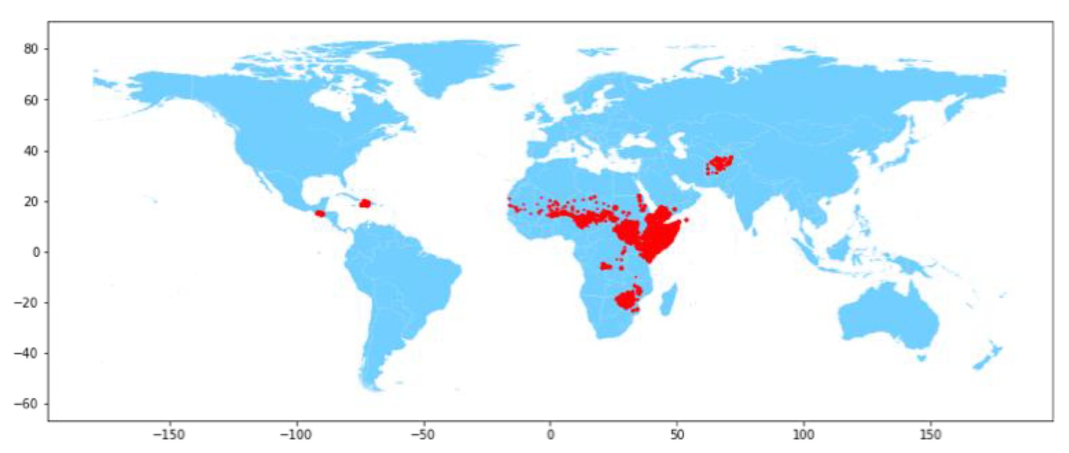
The World Bank dataset contains 21 features of interest and 183,596 observations to be used in the prediction of food crises [12]. The label for the dataset is the presence of a food crisis, as defined by the FEWS NET Integrated Phase Classification (IPC) system (Famine Early Warning Systems Network, n.d.). The IPC is used to help forecast famines in regions around the world through a phased rating system of food insecurity: (1) minimal, (2) stressed, (3) crisis, (4) emergency, and (5) famine (Famine Early Warning Systems Network, n.d.) [13]. IPC ratings are updated every quarter and are recorded at the district level. However, this is a challenging problem to model, and current FEWS NET models fail to classify the majority of food crisis outbreaks with model metrics of recall (0.23), precision (0.42), and f1 (0.30) [10]. The distribution of the response variable is not balanced and strongly favors the absence of a food crisis. As visualized in Figure 1, the majority of food crises are observed across central Africa and are especially concentrated around the horn of Africa. This indicates there is a strong geographic component when considering the potential for a food crisis. While country, district, district code, latitude, and longitude are the geographic features available in the dataset, only latitude and longitude were retained in order to minimize the complexity of the model.
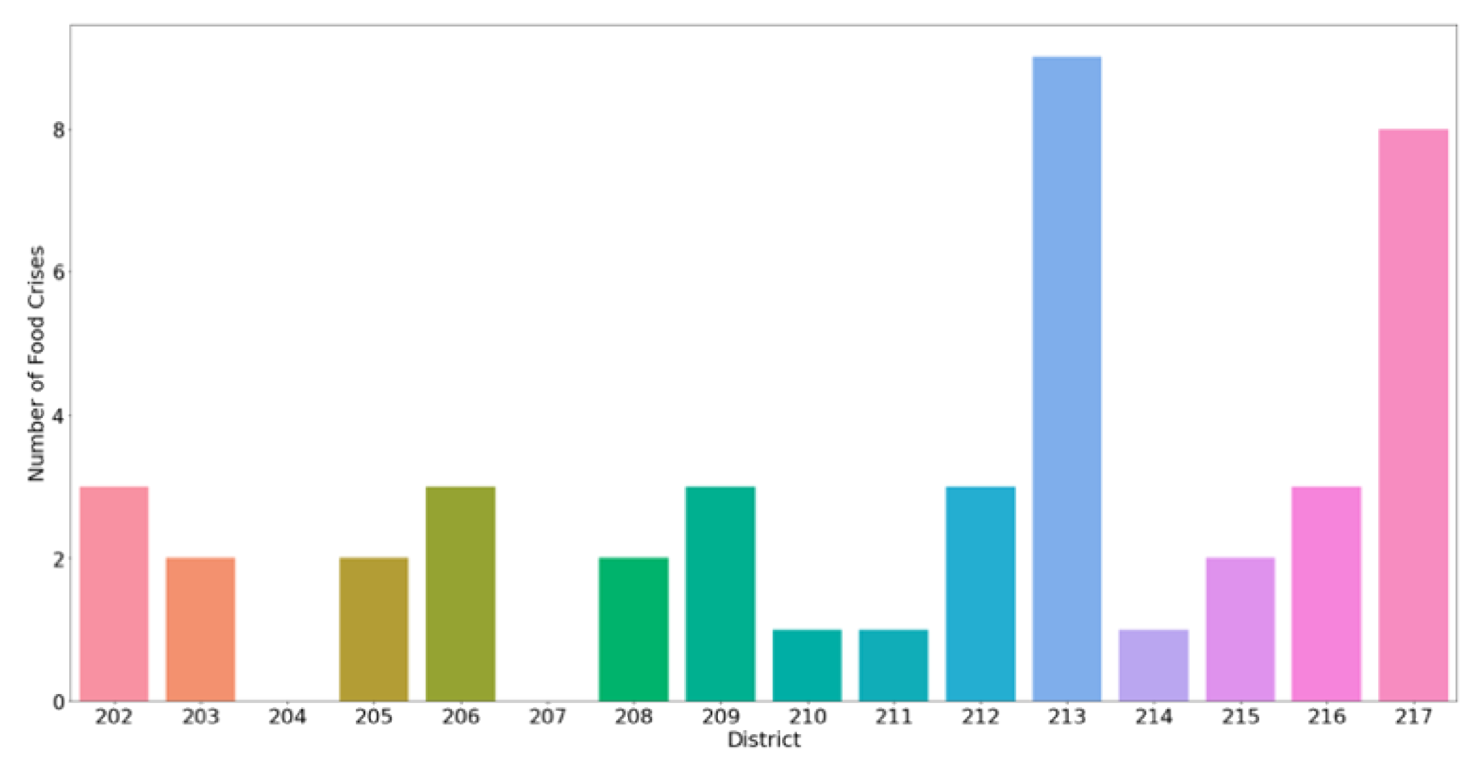
After normalizing the number of food crises by the number of districts per country and by the number of years of observation per country, it was noted that Yemen, South Sudan, and Nigeria had the majority of recorded food crises (52%). Additionally, food crises were not uniformly distributed across a country’s districts, as highlighted in Figure 2, which, as an example, presents a bar chart indicating the number of food crises per district in Afghanistan. In contrast to all the other countries utilized in this dataset, Zambia was the only country that had not recorded a food crisis from 2007 to 2020. In addition to the FEWS NET IPC rating, FEWS NET also indicates which districts are receiving humanitarian assistance. Thus, the presence of humanitarian assistance is likely an indication of an ongoing food crisis.
The World Bank dataset also contains four features regarding near- and medium-term predictions of food crisis and humanitarian assistance. However, these features were removed as data was missing in a significant number of rows. Additionally, one feature containing a combination of year and month was removed as there were separate features for year and month.
The resulting 21 features used to predict food crises in this work are shown in Table 1, along with their range. Selected features are discussed in this section. The normalized difference vegetation index (NDVI) uses satellite imagery to determine the amount and health of vegetation on the earth’s surface and is positively correlated with food production [14]. A feature that tracks the percent deviation from the 20-year NDVI average was incorporated to detect anomalies in vegetation; a value above 1 indicates plant growth and a value below 1 indicates a deficit in plant growth [12]. Two features were added to record the amount of rainfall, measured by the long-term averages of Climate Hazards Group InfraRed Precipitation with Station (CHIRPS), and rainfall required for plant growth, also known as evapotranspiration [15,16]. Both aforementioned variables have a corresponding feature to track anomalies in precipitation and evapotranspiration, respectively [12]. Due to the wide numeric range of population and ruggedness, a log-transformed version of these features was added to the dataset.
Violence has been correlated with food crises and is captured in two features: the number of violent events and the number of fatalities. Africa is the host of several of Foreign Policy’s index of top failed states (Somalia, Chad, Sudan, Zimbabwe, and the Democratic Republic of Congo), and of particular interest, Somalia has been gripped by internal conflicts for the past 20 years [17]. Moreover, an index of food prices was included to quantify food scarcity in the market [18].
The last five features in Table 1 characterize the regions of each country. These features account for the size of the region, the population enclosed, and the amount of pastureland and cropland available. The population and size of the region can help determine the population density and thus help quantify the amount of food needed to be secure. A lack of available cropland and pastureland could indicate a region that is dependent on food imports.
Another potential concern for food security is the loss of cropland and pastureland due to desertification, which is the decrease of the cropland percent feature with time. However, Figure 3 shows these features from 2007 to 2017, which indicates that the amount of cropland has remained constant.
3. Methods
Data preparation and modeling were conducted in Python using a GPU-enabled Google Colaboratory environment and the Scikit-learn, Keras, and TensorFlow frameworks. The cross-industry standard process for data mining (CRISP-DM) was followed, with the phases of data understanding, data preparation, modeling, and evaluation. The data understanding phase is described in the preceding Background section of this paper.
3.1. Data Preparation
The World Bank dataset was cleaned, transformed, and normalized prior to application of logistic regression and neural network methods [12]. For the purpose of this research study, food crises were categorized with a binary target variable of crisis (IPC of 3 or greater) and no crisis (IPC less than or equal to 2).
There were four other data preparation steps conducted prior to modeling:
- A large number of NaN values observed in the FEWS Integrated Phase Classification column and those rows were dropped. This resulted in a significant reduction to approximately 30,000 datapoints.
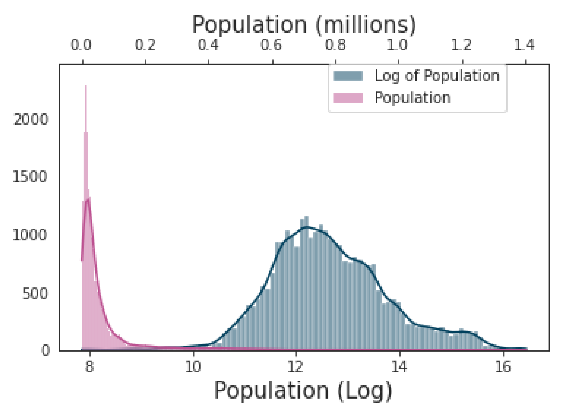
- Log transformations were conducted on the population and the ruggedness index as their histograms indicated they have chi-square distributions. An example showing the impact of the log transformation on the population feature is shown in Figure 4. The untransformed variables were retained in the dataset to capture linear trends.
- All features were normalized in order to increase the learning rate of the machine learning algorithms, with the exception of the country and district categorical variables.
- The month was numerically encoded with January represented as 1 and December represented as 12.
3.2. Metrics
In this analysis, the classification metrics of precision, recall, and f1 were used to measure the performance of the classical and neural network models. In the dataset, the positive class is a food crisis. In the case of an actual food crisis, it is critical that a model prediction of no food crisis be avoided. As a result, recall is the most important metric, which helps to avoid false negatives. Precision was also selected as accurate predictions of true positives are important, and f1 was chosen due to the unbalanced nature of the dataset where only 15.3% of labels are positive. These three metrics also facilitated a direct comparison to prior work. In certain cases, the area under the receiver operating characteristic curve (AUC) and accuracy are also presented to highlight differences between models.
3.3. Classical Modeling
Logistic regression was performed on the full dataset and on features selected using p-value selection, recursive feature elimination (RFE), and select k-best methods. For feature selection, these algorithms were used as the large number of features made investigating all possible feature combinations computationally prohibitive. The goal of the feature selection process is to create the simplest model with the highest level of performance in order to ensure the model is interpretable and can generalize well on unseen data.
Performance was evaluated using accuracy, precision, recall, and f1 metrics. Overfitting was monitored using a train/validate split of 66%/33%. It was verified that both the train and validate sets contained an equal stratification of food crises (15.3%).
3.4. Neural Network Modeling
The neural network modeling effort utilized the binary cross-entropy loss function to maximize the effectiveness of the binary classification algorithm. Root mean squared propagation (RMSprop) and adaptive moment estimation (Adam) were evaluated as optimizers for the model. Due to the size of the dataset and the number of input features, a three-way data split was utilized over cross-validation in order to minimize the computational demand. The modeling effort was monitored for overfitting using a 70%/15%/15% train/test/holdout split. A checkpointing algorithm was used during training, which saved the model each time the loss metric on the test dataset improved; this ensured the best possible performance was realized. Similar to the logistic regression model, it was verified that all datasets contained an equal stratification of food crises, and the performance was evaluated using accuracy, precision, recall, and f1 metrics. The f1 is the harmonic mean of precision and recall, as defined by Equation (1).
The holdout dataset was needed due to the high model capacity of the neural network and the large number of variations that were attempted. Due to this process, it is likely that the test dataset was inadvertently optimized, even though it was not used in the neural network backpropagation calculations. The holdout dataset ensures that the model can generalize well on unseen data.
Five iterations of neural network modeling were conducted. The first iteration was the baseline neural network, which consisted of a single input layer, a normalization layer, two hidden layers with 150 ReLu neurons each, and an output layer with one sigmoid neuron. The second iteration consisted of a series of single hyperparameter sweeps to determine the optimal optimizer, number of training iterations, learning rates, classification thresholds, and the number of hidden layers and neurons per layer. The model’s recall, precision, accuracy, and f1 were recorded to evaluate the effectiveness of each of the hyperparameters tested.
Iteration 3: The results of iteration 2 modeling informed the iteration 3 multidimensional hyperparameter search, which was conducted using variations of architecture, compilation, and training hyperparameters. The Adam optimizer epsilon parameter was specified as 0.0001, and the hyperparameter variation space is detailed in Table 2.
Two variations of series 3 were run: a high batch variation that limited the batch size to 2048 and 4096 and a low batch variation that contained batch sizes 32–1024. Each high batch model trained in 1–2 min, and each low batch model took as long as 15 min to train. The high batch results were used to shape the multidimensional search for the low batch modeling effort. An iterative multidimensional hyperparameter search following the process flowchart shown in Figure 5 was followed and repeated until the performance changed by less than 2%. In the flowchart, initial hyperparameters (HP) and their ranges are selected from the literature [19].
Iteration 4: This iteration repeated the iteration 3 high batch modeling effort with an architecture variation. Instead of a flat stack of neural network layers where all layers contain the same neuron count, the layers were tapered. With the exception of the output layer, every layer contained half the neuron count of the preceding layer. For example, if the first layer contained 100 neurons and there were two hidden layers, the neuron count of the layers would be 100, 50, 25, and 1. The iterative multidimensional hyperparameter search from Figure 5 was followed.
Iteration 5: Due to the high capacity of the neural networks used, it was possible that the neural network could memorize the historical dataset. While the train/test/holdout approach assured the researchers that the model could generalize well on unseen historical data, a concern was that the model would be unable to generalize well on future data. Application of the model will be on future data, where the year is outside of range of the dataset, causing the model to extrapolate. For these reasons, the iteration 5 multidimensional hyperparameter search was repeated after the “year” feature was removed from the dataset. The architecture of this iteration was the same as iterations 1–3, and the Figure 5 flowchart was followed.
4. Results
Logistic regression and neural network models were developed and evaluated based on their ability to accurately predict food crises while minimizing false positives and false negatives.
4.1. Logistic Regression Model
First, the full model was built with all the features found in Table 1. In the full model, all features were found to be statistically significant (p < 0.05) except for NDVI (p = 0.288), NDVI anomalies (p = 0.357), and evapotranspiration anomalies (p = 0.051). From here, features were eliminated on the basis of p-value, with the goal of minimizing model complexity while maintaining performance. After paring down the model, the p-value selection model yielded the following features with p < 0.001: month, food assistance, mean evapotranspiration, number of violent events, food price index, and the cropland percent. The presence of humanitarian assistance was the feature most strongly associated with a food crisis (coefficient: 0.62). Month was the feature that was most negatively correlated with a food crisis (coefficient: −0.12). The remaining features had coefficients that were relatively small (<0.1) and had less influence on the model. In Table 3, the accuracy (0.86), recall (0.16), and precision (0.81) of the model is indicative of a trivial model that only predicts food crises.
Then, recursive feature elimination (RFE) was conducted to create models ranging 7–11 features. All RFE models had the following features in common: humanitarian assistance, mean evapotranspiration, number of violent events, and latitude. After testing each of the five models suggested by RFE, there was not a significant difference between the ROC curve, accuracy, recall, and precision. Thus, the simplest model was selected with the following features: latitude, month, humanitarian assistance, food price index, number of violent events, and cropland percent. All selected featured had p < 0.001. The inferences from this model were that humanitarian assistance was most strongly correlated with food crises (coefficient: 0.73), and month was most strongly negatively correlated with food crises (coefficient: −0.11). Although different features were utilized in the RFE model, the model performance was identical to the performance of the p-value selection model. These metrics are also shown in Table 3.
The last feature selection technique utilized was select k-best. After creating models with 7–11 features, the following model features were found to be statistically significant with p < 0.001: year, month, mean NDVI, mean rainfall, mean evapotranspiration, number of violent events, price index of food, cropland percent, log population, and log ruggedness index. The price index of food and the mean NDVI were the most positively correlated with food crises. In this model, mean evapotranspiration and the log population were the most negatively correlated with food crises. As seen in Table 3, the select k-best model, in comparison to the previous logistic regression models, slightly increased the model’s AUC (0.59), recall (0.20), and accuracy (0.87) while slightly decreasing the model’s precision (0.75).
Additionally, Table 3 provides a set of hypothetical models that assist in evaluating the models developed in this work:
- Chance: metrics that result if the model predicts randomly.
- Always predicts crisis: a model that always predicts the minority class or food crisis.
- Never predicts crisis: a model that always predicts the majority class or no food crisis. This is also known as the no information rate (NIR).
- Goal/prior work: the performance metrics from the model developed by World Bank researchers (Andree, Chamorro, Kraay, Spencer, and Wang, Predicting Food Crises. Policy Research Working Paper; no 9412, 2020).
4.2. Neural Network Model
Five iterations of neural network modeling were conducted in this work. A summary of their performance metrics is located in Table 4 at the end of this section.
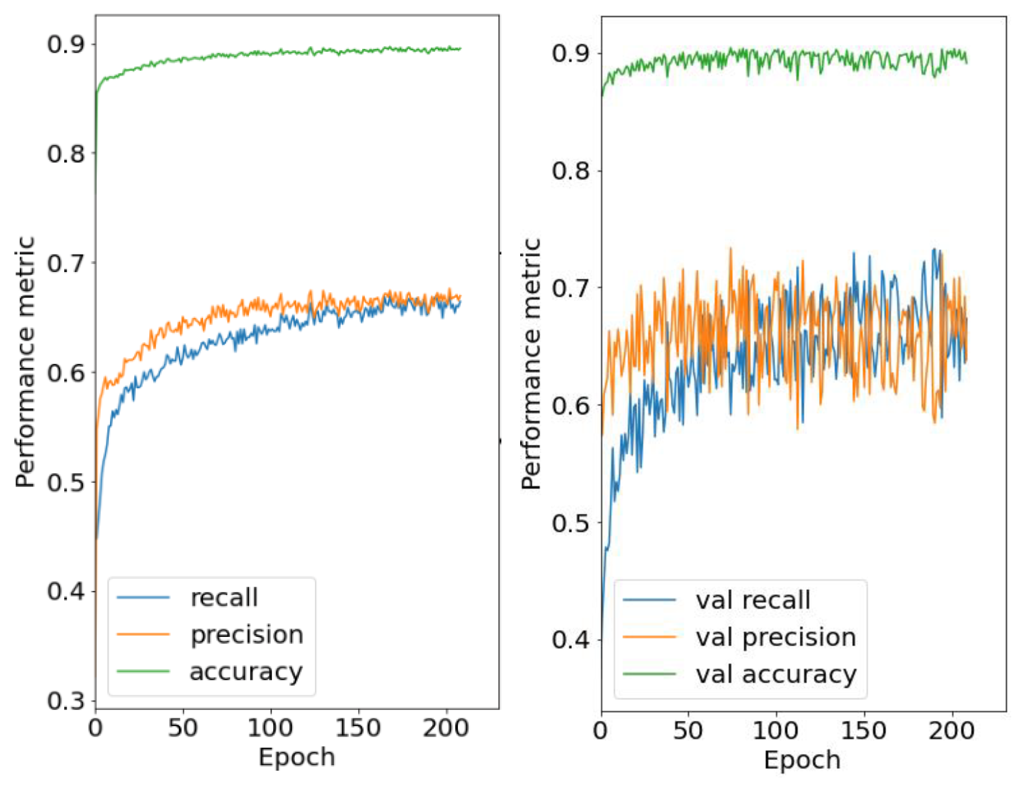
Iteration 1 baseline: The baseline neural network consisted of one input layer, a normalization layer, two 150-neuron ReLu hidden layers, one sigmoid output layer, and the RMSprop optimizer with a 0.0001 learning rate. Training was conducted with 1000 epochs, and the early stopping patience parameter was set to 50. The training curves for iteration 1 are shown in Figure 6, and they show that even though the training recall (left) continued to improve with additional training epochs, the recall for the validation set indicated overfitting as it started to degrade after 25 epochs.
Iteration 2: In this iteration, single-hyperparameter sweeps were conducted to explore the hyperparameter space. The learning rate was swept from 0.00001 to 0.01, resulting in an optimal recall and precision at a learning rate of 0.001. Then, the number of training iterations were swept from 10 to 200 using the RMSProp optimizer algorithm. This showed that precision increased linearly with training, while recall increased linearly before reaching a plateau at approximately 100 iterations. The training iteration sweep was then repeated with the Adam optimizer, and the recall and precision increased logarithmically and plateaued at around 200 iterations. The Adam optimizer was ultimately selected because it achieved the highest recall and precision and was less prone to overtraining in comparison to RMSprop.
Sweeping the classification threshold from 0.10 to 0.90 revealed that the optimal classification threshold was approximately 0.30. A lower classification threshold favors recall, while a higher threshold favors precision. Then, the number of hidden layers (1–2) and the number of neurons (25–200) were varied, and it was identified that a model with 2 hidden layers and 150 neurons each optimized the model’s precision and recall. A model utilizing the optimized hyperparameters exhibited the following performance metrics for predicting food crises: accuracy (0.88), AUC (0.83), recall (0.76), and precision (0.60).
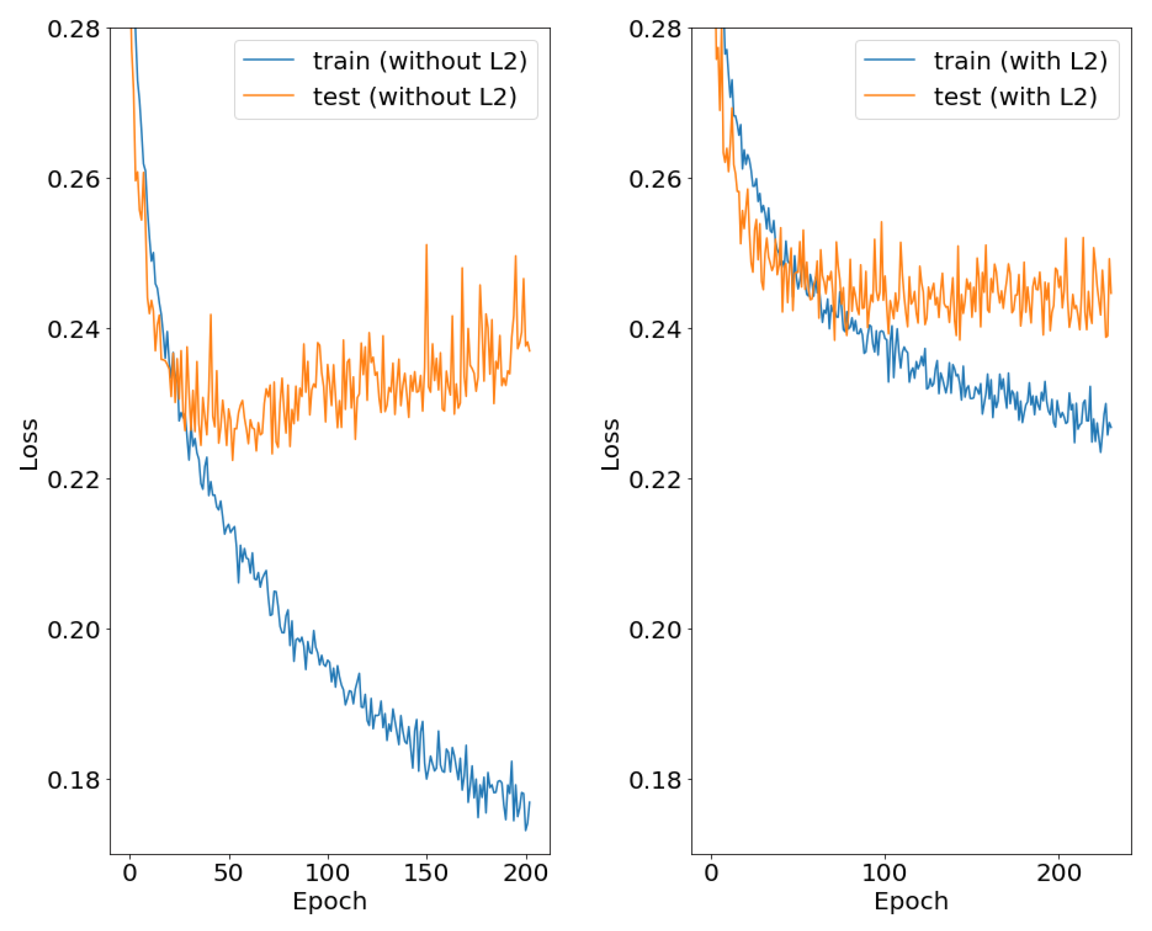
The effects of L2 regularization on model performance were investigated due to the large neuron count of the model. As seen in Figure 7 (left), the model without regularization overtrained quickly. Next, L2 regularizers were added to the hidden layers, and the regularization factor was swept from 0.00001 to 0.01 to find the optimal value (0.0001). As shown in Figure 7 (right) and Table 4, the addition of L2 regularization appeared to stabilize the training of the model and prevented overfitting without substantially changing model performance. The model performance metrics were as follows: accuracy (0.88), AUC (0.83), recall (0.74), and precision (0.60).
Iteration 3: Multidimensional hyperparameter sweeps: Significant gains in model performance were attained with the multi-dimensional hyperparameter sweep. A total of 920 networks were trained in the high batch variation, and 660 networks were trained in the low batch variation.
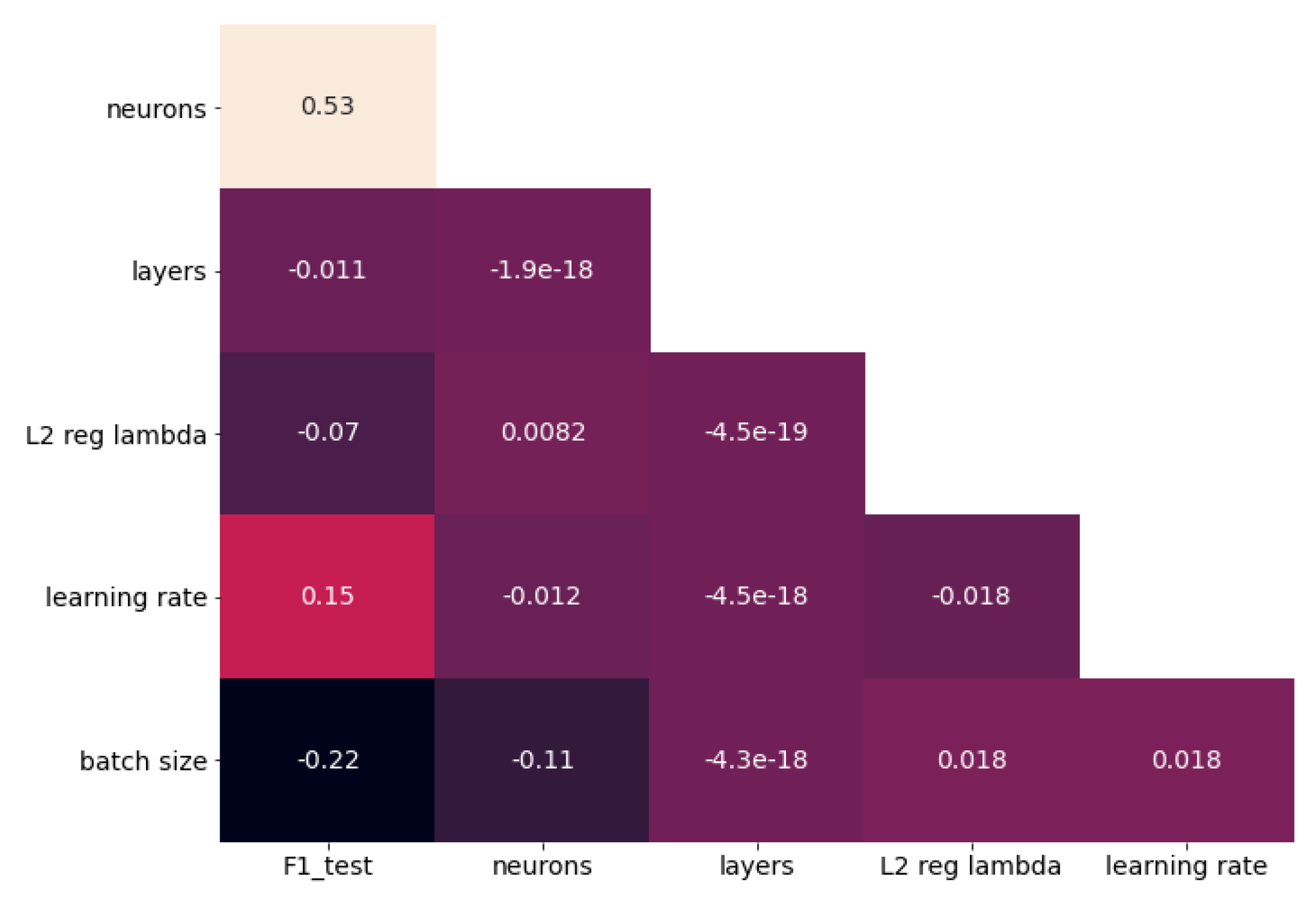
Using the f1 metric of the test set as the dependent variable, hyperparameter correlation was examined and is presented in Figure 8. Within the hyperparameter space examined, neuron count had the biggest linear impact on f1, followed by batch size and learning rate. It is notable that while model capacity (in terms of the number of weights) would be most affected by the number of layers, Figure 8 indicates that it had the smallest impact on model performance.
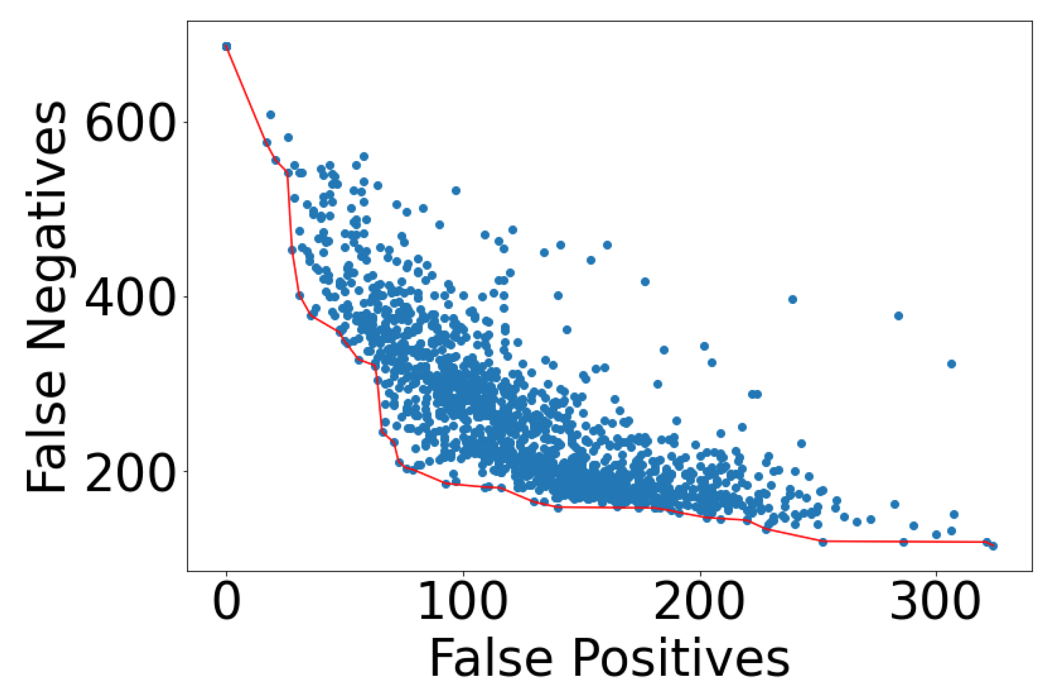
A wide range of modeling performance resulted when the counts of false negatives (FN) and false positives (FP) were examined. Many of the models arrived at a trivial solution, with the model overspecifying either FP or FN in order to achieve a low value on its compliment. In Figure 9 below, all model FN and FP results for the test set are reported, with a red line indicating the Pareto front, which is the best family of models. These models contain the lowest FN count for each value of FP.
There were 658 food crisis in the training set, and a trivial model is shown on the left side of Figure 9, with 0 FP and 658 FN. At the other extreme, the lowest value of FN was 158 (of 3800); however, that model misclassified half of the food crises, resulting in a FP of 324.
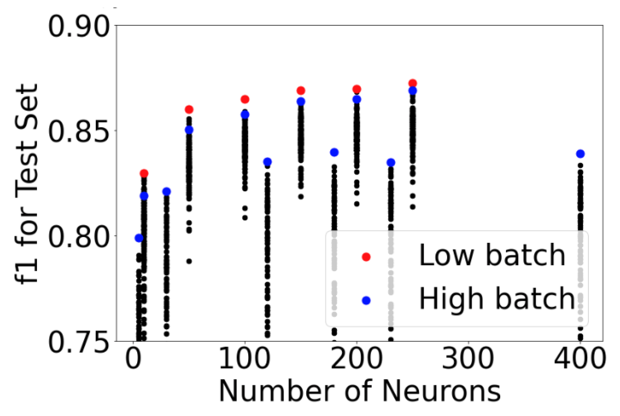
The impact of individual hyperparameters on the f1test metric were then examined, starting with neuron count. As shown in Figure 10, the best model performance was achieved at a neuron count of 250; however, only incremental improvement occurred once the neuron count surpassed 50. Moreover, the impact of batch size on performance can be clearly seen, with the red markers in Figure 10 showing the best performance for the low batch variation and the blue markers reporting performance for the high batch variation. The low batch variation (≤1024) surpassed the performance of the high batch variation (2048 or 4096) in every case.
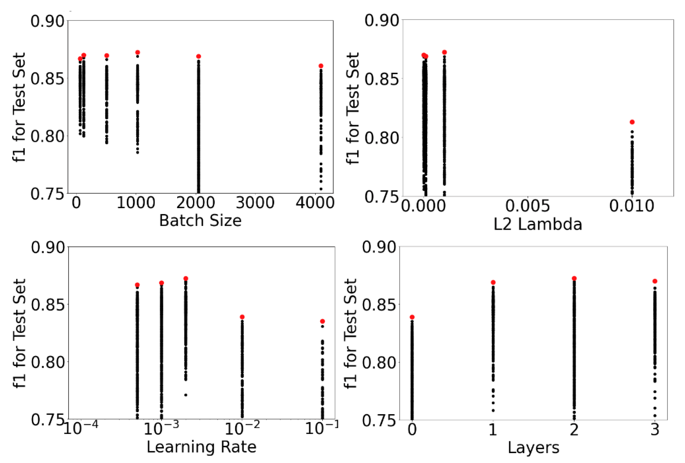
Figure 11 reports the f1test metric for the other hyperparameters. Local maximums were apparent for the batch size, L2 regularization parameter, and learning rate, while any layer count ≥1 had equivalent performance.
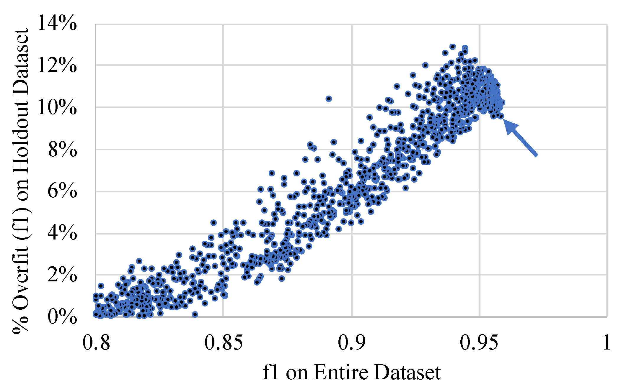
When examining the level of performance between the f1 metrics of the entire dataset and the holdout dataset, a quasi-linear overfitting relationship was observed. This relationship is presented in Figure 12, along with an arrow that shows the best model that meets the 10% overfitting threshold.
Iteration 4: Multiple hyperparameter sweeps (tapered stack): Finally, a subset of the iteration 3 hyperparameter search was repeated using the architecture modification discussed in Section 3. While this iteration used the full dataset, its performance (f1test = 0.84) was equivalent to the “no year” modeling. This indicated that this series of models was not useful, and they are not discussed further.
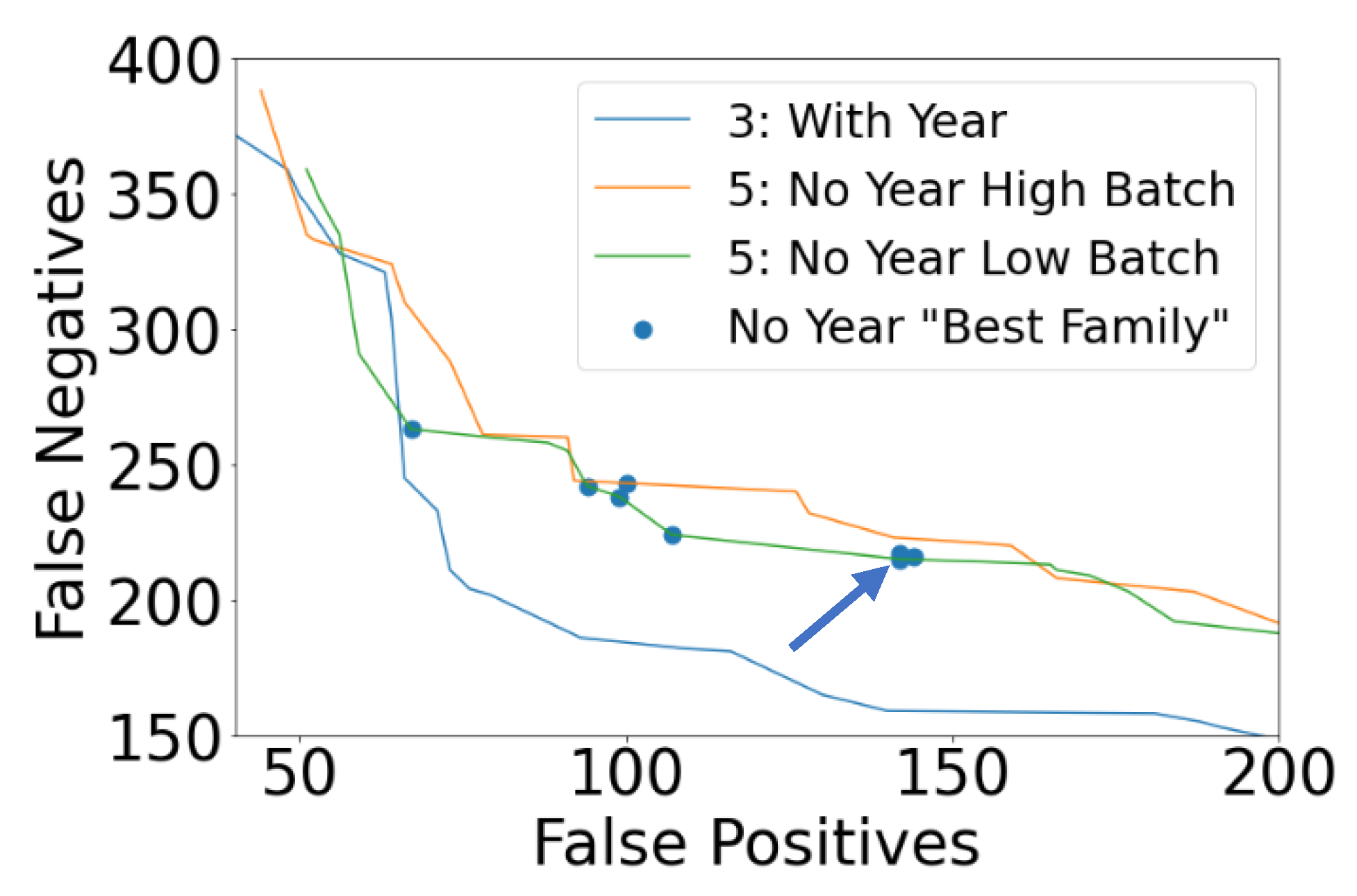
Iteration 5: Multiple hyperparameter sweeps (no year): Similar to iteration 3, high batch and low batch variations of modeling the “no year” dataset were conducted, and the low batch variation had the best performance. Removing the year feature had the impact of slightly degrading model performance, as shown in Figure 13. In the figure, the Pareto front from “with year” dataset in iteration 3 is plotted (blue), along with two Pareto fronts from iteration 5, namely orange for high batch and green for low batch. It is notable that for the “no year” dataset, models with FP < 65 yielded equivalent performance to the “with year” dataset. However, as the number of FP increased, there was noticeable degradation in the FN count.
The final step in model selection was to select a best family of iteration 5 models and compare them to the holdout dataset. The models were ranked by the f1 metric on the entire dataset, and the model performance was then evaluated for false negatives, which is a priority for this application. Eight models were selected. Table 4 shows the hyperparameters associated with these models and their f1 performance on the entire/test/holdout datasets.
Finally, models were excluded if their f1 metric on either the test or holdout set was more than 10% lower than the f1 metric on the entire dataset. This ensured that the model would be able to generalize well on unseen data. The best model is denoted by bold text in Table 4, and while it did not have the highest f1all, it performed well and met all criteria. Further metrics for the best model are presented in Table 5.
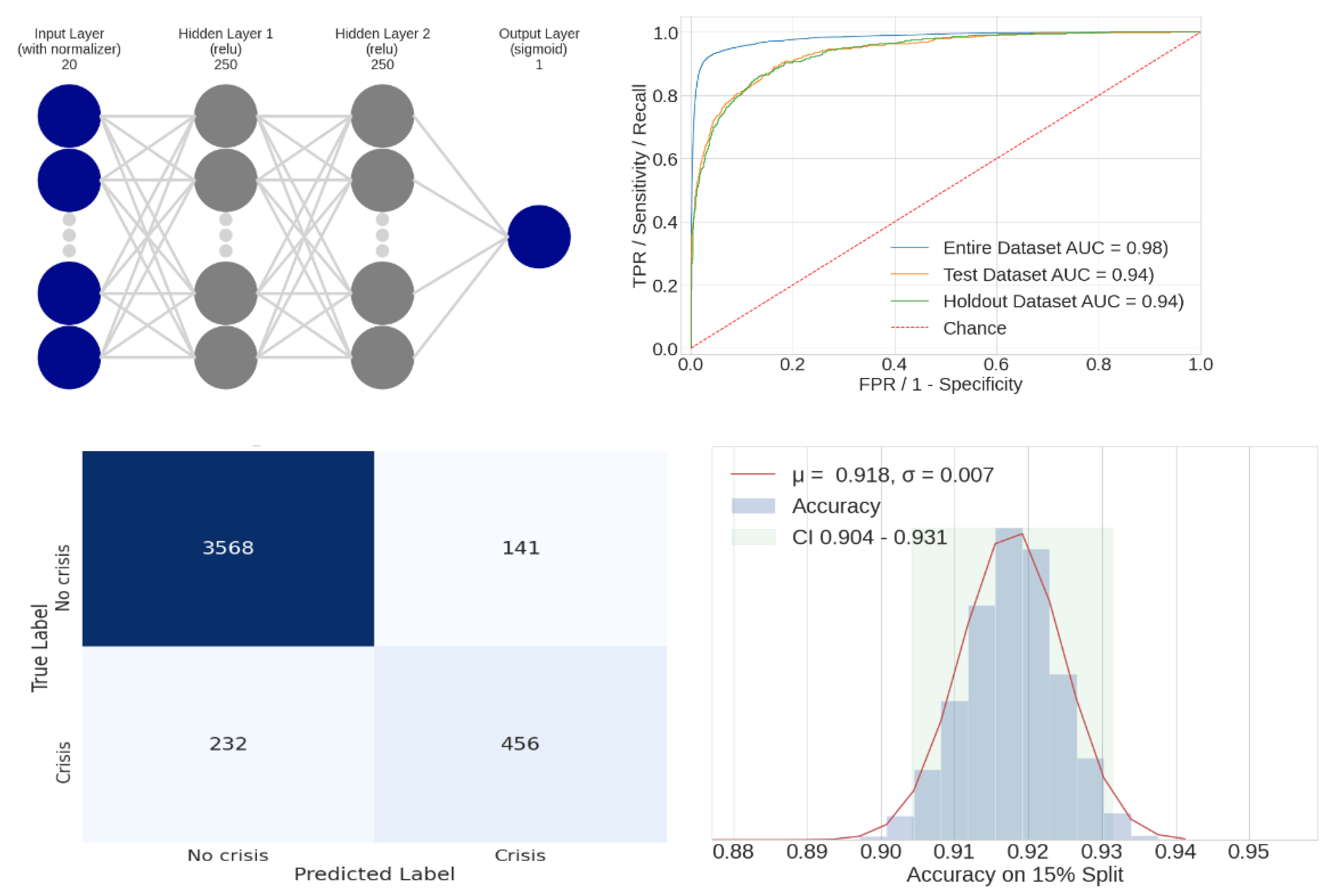
Additional information on the final model is presented in Figure 14, which displays the neural network structure, confusion matrix, and ROC AUC. Figure 14 also contains a statistical analysis of the recall primary performance metric, and additional background on the analysis follows. The validation and holdout datasets each consisted of a random 15% portion of the original dataset, as determined by a specified random seed. A sensitivity analysis was performed by recording the recall metric for a 15% split that resulted from 1500 different random seed values. The resulting histogram is shown in Figure 14 (bottom left), showing a normal distribution and a recall mean value of 0.92 with a 95% CI of ± 0.01. This gives confidence that there was a relatively even distribution of outliers in the dataset; the CI would have been larger if that was not the case. As expected, the mean value of the 15% split histogram matched the recall of the entire dataset.
Iteration 1–5 summary: A summary table of all neural network modeling iterations is presented in Table 6, which was measured on the test dataset. When comparing iterations 3 and 5, it is notable that there was minimal effect of removing year from the data set.
4.3. Discussion
For all models, recall must be high (>0.80) to ensure most food crises are predicted accurately, but without maintaining precision (>0.80), the significance of the model predictions would be diluted. When considering these goals, the performance metrics for the logistic regression models indicate they are not useful. While the optimal select k-best model was statistically significant, its AUC (0.59) performed only 9% better than the chance hypothetical model that is shown in Table 3. Additionally, the model’s f1 (0.32) represented a 37% decrease from the goal model performance. The model’s precision (0.75) indicated that 25% of the food crises classified as food crises were false positives; furthermore, the model’s recall (0.20) indicated the model failed to classify 80% of the food crises in the dataset. These performance metrics suggest that the logistic regression models generalize to the trivial solution of not predicting food crises. This is further evidenced by the model’s accuracy (0.87), which only performed 2% better than a model that did not classify food crises (Table 3). Thus, the logistic regression model cannot be considered a viable model and does not meet the performance goals outlined for evaluating the model.
Although the logistic regression models did not prove meaningful for prediction, they yield valuable inferences that the presence of humanitarian assistance and the food price index are potential indicators of food crises. These features may be an indicator of a systemic government crisis and could prove meaningful for future study.
The neural network models vastly outperformed the logistic regression models. The most striking improvement was in the best neural network model’s AUC (0.98), which was 66% better than the logistic regression models and 96% better than a pure chance model. When considering performance on the unseen holdout dataset, the best NN model’s precision (0.85) and f1 (0.83) significantly improved upon the goal model performance by 139% and 68%, respectively, while maintaining recall (0.81) and accuracy (0.92).
Moreover, of critical significance, the best neural network model was developed to be year agnostic and maintained a f1 on the test (0.84) and holdout (0.83) sets, thereby suggesting that the model has the capability to extrapolate on future data. The main limitation of this work is the potential for the model to misclassify a food crisis. When this model is applied to future data, the 0.82 recall on the holdout dataset indicates that nearly 1 in 5 food crises will be misclassified. This indicates that it is essential for governments and aid organizations to verify current conditions prior to making a decision based on this model.
5. Conclusions
The project aimed to predict food crises in 21 countries between 2007 and 2020 based on 21 predictive features from a World Bank dataset. Using the CRISP-DM process, the data was cleaned, normalized, modeled, and evaluated utilizing logistic regression and neural network models. The results demonstrated that neural network models could successfully predict food crises, while the logistic regression models proved to be largely unsuccessful. The neural network model significantly outperformed a pure chance model, with an 88% increase in AUC and nearly 3× improvement in f1. The NN model also outperformed the goal performance metrics by 139% for precision and 58% for f1 while maintaining recall (Table 6). Furthermore, the neural network model was developed to be year agnostic and represents a novel approach to predict food crises from extrapolated data. The near identical performance on the f1 test (0.84) and f1 holdout (0.83) datasets suggests the model can generalize well to unseen data and is critical for model viability. The neural network modeling effort successfully improves upon existing food crisis prediction efforts by FEWS NET and the random forest developed by researchers at the World Bank and may be a valuable tool for governments to target humanitarian aid. As other classifiers and neural network architectures become established, a future extension of this work could be to remodel the dataset in an attempt to further improve model performance. Elements of probabilistic logic graphs have been used to approximate difficult problems and may be useful in this case [20]. Additionally, a study could be conducted that applies this model on future data to further validate its performance.
Authors’ Note: The views and opinions of authors expressed herein do not necessarily state or reflect those of the U.S. Government or any agency thereof. Reference to specific commercial products does not constitute or imply its endorsement, recommendation, or favoring by the U.S. Government. The authors declare this is a work of the U.S. Government and is not subject to copyright protections in the United States. This article was cleared with case number 88ABW-2021-0328.
Author Contributions
Conceptualization, C.C. and T.W.; methodology, C.C., T.W. and B.L.; software, C.C. and T.W.; validation, C.C. and T.W.; formal analysis, C.C. and T.W.; investigation, C.C.; resources, T.W.; data curation, C.C.; writing—original draft preparation, C.C. and T.W.; writing—review and editing, T.W. and B.L.; visualization, C.C. and T.W.; supervision, T.W. and B.L.; project administration, T.W. and B.L. All authors have read and agreed to the published version of the manuscript.
Funding
This research received no external funding, and the article processing charge was funded by the Air Force Institute of Technology.
Data Availability Statement
The data used in this study is publicly archived [12].
Conflicts of Interest
The authors declare no conflict of interest.
References
- Kissinger, H. World Order; Penguin Press: New York, NY, USA, 2014. [Google Scholar]
- Kaplan, R.D. The Return of Marco Polo’s World: War, Strategy, and American Interests in the Twenty-First Century; Random House: New York, NY, USA, 2018. [Google Scholar]
- Department of Defense. Summary of the National Defense Strategy; Department of Defense: Washington, DC, USA, 2018.
- Zeihan, P. Disunited Nations: The Scramble for Power in an Ungoverned World; Harper Business: New York, NY, USA, 2020. [Google Scholar]
- Wischnath, G.; Bahaug, H. Rice or riots: On food production and conflict severity across India. Political Geogr. 2014, 43, 6–15. [Google Scholar] [CrossRef] [Green Version]
- Huang, J.; Zhang, G.; Zhang, Y.; Guan, X.; Wei, Y.; Guo, R. Global desertification vulnerability to climate change and human activities. Land Degrad. Dev. 2020, 31, 1380–1391. [Google Scholar] [CrossRef]
- Whitmire, C.; Vance, J.; Rasheed, H.; Missaoui, A.; Rasheed, K.; Maier, F. Using Machine Learning and Feature Selection for Alfalfa Yield Prediction. AI 2021, 2, 71–88. [Google Scholar] [CrossRef]
- Wen, W.; Timmermans, J.; Chen, Q.; van Bodegom, P. A Review of Remote Sensing Challenges for Food Security with Respect to Salinity and Drought Threats. Remote Sens. 2020, 13, 6. [Google Scholar] [CrossRef]
- Sousa, D.; Small, C. Mapping and Monitoring Rice Agriculture with Multisensor Temporal Mixture Models. Remote Sens. 2019, 11, 181. [Google Scholar] [CrossRef] [Green Version]
- Andree, B.P.; Chamorro, A.; Kraay, A.; Spencer, P.; Wang, D. Predicting Food Crises. Policy Research Working Paper; no 9412. Available online: https://openknowledge.worldbank.org/handle/10986/34510 (accessed on 16 December 2020).
- Moscato, V.; Picariello, A.; Sperlí, G. A benchmark of machine learning approaches for credit score prediction. Expert Syst. Appl. 2021, 165, 113986. [Google Scholar] [CrossRef]
- Andree, B.P.; Chamorro, A.; Kraay, A.; Spencer, P.; Wang, D. Afghanistan, Burkina Faso, Chad, Congo, Dem. Rep., Ethiopia, Guatemala, Haiti, Kenya, Malawi, Mali, Mauritania, Mozambique, Niger, Nigeria, Somal—Predicting Food Crises 2020, Dataset for reproducing working paper results. Available online: https://microdata.worldbank.org/index.php/catalog/3811/data-dictionary (accessed on 11 November 2020).
- Famine Early Warning Systems Network. Integrated Phase Classification. Available online: https://fews.net/IPC (accessed on 11 November 2020).
- National Aeronautics and Space Administration. Earth Observatory. 30 August 2000. Available online: https://earthobservatory.nasa.gov/features/MeasuringVegetation/measuring_vegetation_3.php (accessed on 27 January 2021).
- Belay, A.S.; Fenta, A.A.; Yenehun, A.; Nigate, F.; Tilahun, S.A.; Moges, M.M.; Dessie, M.; Adgo, E.; Nyssen, J.; Chen, M.; et al. Evaluation and Application of Multi-Source Satellite Rainfall Product CHIRPS to Assess Spatio-Temporal Rainfall Variability on Data-Sparse Western Margins of Ethiopian Highlands. Remote. Sens. 2019, 11, 2688. [Google Scholar] [CrossRef] [Green Version]
- US Geological Survey. Evapotranspiration and the Water Cycle. Available online: https://www.usgs.gov/special-topic/water-science-school/science/evapotranspiration-and-water-cycle?qt-science_center_objects=0#qt-science_center_objects (accessed on 11 May 2021).
- Kimenyi, M.S.; Mlbaku, J.M.; Moyo, N. Reconstituting Africa’s Failed States: The Case of Somalia. Soc. Res. 2010, 77, 1339–1366. [Google Scholar]
- INDDEX Project. Data4Diets: Building Blocks for Diet-Related Food Security Analysis. Tufts University, INDDEX Project. Available online: https://inddex.nutrition.tufts.edu/data4diets (accessed on 27 January 2021).
- Géron, A. Hands-On Machine Learning with Scikit-Learn and TensorFlow: Concepts, Tools, and Techniques to Build Intelligent Systems, 2nd ed.; O’Reilly Media, Inc.: Sebastopol, CA, USA, 2019. [Google Scholar]
- Han, Q.; Molinaro, C.; Picariello, A.; Sperli, G.; Subrahmanian, V.S.; Xiong, Y. Generating Fake Documents using Probabilistic Logic Graphs. IEEE Trans. Dependable Secur. Comput. 2021, 1. [Google Scholar] [CrossRef]
Figure 1.
Mapping food crises in countries analyzed using FEWS NET IPC.

Figure 2.
Food crises per district (showing 16/34 districts) in Afghanistan from 2007 to 2020.

Figure 3.
Percent cropland for countries over time.

Figure 4.
Population feature as measured in millions (left side, top x axis) and normalized with log transformation (center, bottom x axis).
Figure 4.
Population feature as measured in millions (left side, top x axis) and normalized with log transformation (center, bottom x axis).

Figure 5.
Flowchart for iterative multidimensional hyperparameter search. HP: hyperparameter; HOML: Hands-On Machine Learning with TensorFlow [19].
Figure 5.
Flowchart for iterative multidimensional hyperparameter search. HP: hyperparameter; HOML: Hands-On Machine Learning with TensorFlow [19].

Figure 6.
Training (left) and validation (right) curves for model trained with RMSprop.

Figure 7.
Training and validation loss curves: model without L2 regularization (left) and model with L2 regularization (right).
Figure 7.
Training and validation loss curves: model without L2 regularization (left) and model with L2 regularization (right).

Figure 8.
Correlation between hyperparameters and f1 (test).

Figure 9.
Investigating the tradeoff between FN (test) and FP (test) on 1580 candidate models, with the red line indicating the Pareto front and the best family of models.
Figure 9.
Investigating the tradeoff between FN (test) and FP (test) on 1580 candidate models, with the red line indicating the Pareto front and the best family of models.

Figure 10.
Effect of neuron count and batch size on f1 for the test set.

Figure 11.
Effect of batch size (top left), L2 lambda (top right), learning rate (bottom left), and layers (bottom right) on the f1 parameter.
Figure 11.
Effect of batch size (top left), L2 lambda (top right), learning rate (bottom left), and layers (bottom right) on the f1 parameter.

Figure 12.
Relationship between the f1 metric of the entire dataset and the percent decrease of the f1 metric on the holdout dataset (overfitting). An arrow indicates the best model that meets the 10% overfitting threshold.
Figure 12.
Relationship between the f1 metric of the entire dataset and the percent decrease of the f1 metric on the holdout dataset (overfitting). An arrow indicates the best model that meets the 10% overfitting threshold.

Figure 13.
Resulting Pareto fronts for the “with year” dataset (iteration 3, blue), “no year” dataset with high batch count (iteration 5, orange), and “no year” dataset with low batch count (iteration 5, green). The blue dots indicate the best family of models from iteration 5, and the blue arrow indicates the best iteration 5 model.

Figure 14.
Final neural network model structure (top left), receiver operating characteristic AUC for the entire/test/holdout datasets (top right), confusion matrix for the holdout dataset (bottom left), and statistical analysis of the recall metric for the holdout dataset (bottom right). RELU: rectified linear unit; TPR: true positive rate; FPR: false positive rate.


Table 1.
Dataset summary.
| Parameter | Range |
|---|---|
| Latitude (deg) | −91.931–71.456 |
| Longitude (deg) | −25.862–37.038 |
| Month | January–December |
| Year | 2007–2020 |
| Food assistance | 0 or 1 |
| Vegetation index (NVDI) | −0.043–0.86 |
| NVDI anomalies | −5496–3790 |
| Mean rainfall | 0.0–125.92 |
| Rain anomalies | −42.51–80.80 |
| Mean evapotranspiration | 0.0–47.90 |
| Evapotranspiration anomalies | −17.50–17.11 |
| Violent events (#) | 0.0–256 |
| Fatalities (#) | 0.0–2394 |
| Food price index | 0.20–139.0 |
| Population (#) | 2123–14,050,940 |
| Log(population) | 7.8–16.4 |
| Cropland percent (%) | 0.0–99.24 |
| Pastureland percent (%) | 0.0–99.60 |
| Ruggedness index | 134.9–1,046,065 |
| Log(ruggedness) | 1.3–13.9 |
| Area (sq. mi.) | 10.29–331,292 |
Table 2.
Neural network model hyperparameters and search range.
| Parameter | Specification |
|---|---|
| Neuron count | 5, 10, 30, 50, 100, 120, 150, 180, 200, 230, 250, 400 |
| Layer count | 0, 1, 2, 3 |
| L2 regularization λ | 0, 0.0001, 0.0005, 0.001, 0.01 |
| Batch size | 32, 64, 128, 512, 1024, 2048, 4096 for high batch |
| Epochs | 400–1000 (checkpointed) |
| Learning rate | 0.0001–0.1 |
Table 3.
Logistic regression model metrics as measured on the test dataset. Grey text indicates three hypothetical models that assist in model evaluation.
Table 3.
Logistic regression model metrics as measured on the test dataset. Grey text indicates three hypothetical models that assist in model evaluation.
| Model | p-Value | AUC | Precision | Recall | Accuracy | f1 |
|---|---|---|---|---|---|---|
| Full | 0.00 | 0.58 | 0.73 | 0.18 | 0.86 | 0.29 |
| p-Value Selection | 0.00 | 0.58 | 0.81 | 0.16 | 0.86 | 0.27 |
| RFE | 0.00 | 0.58 | 0.81 | 0.16 | 0.86 | 0.27 |
| Select k-best | 0.00 | 0.59 | 0.75 | 0.20 | 0.87 | 0.32 |
| Chance | -- | 0.50 | 0.15 | 0.50 | 0.50 | 0.23 |
| Always predicts crisis | -- | -- | 0.15 | -- | 0.15 | -- |
| Never predicts crisis | -- | -- | -- | -- | 0.85 | -- |
| Goal/prior work (Andree, Chamorro, Kraay, Spencer, and Wang, Predicting Food Crises. Policy Research Working Paper; no 9412, 2020) | -- | -- | 0.36 | 0.84 | 0.91 | 0.50 |
Table 4.
Hyperparameters and f1 metrics for the best family of NN models. Metrics are presented for the entire dataset, test dataset, and holdout dataset. The selected best model is denoted by bold text.
Table 4.
Hyperparameters and f1 metrics for the best family of NN models. Metrics are presented for the entire dataset, test dataset, and holdout dataset. The selected best model is denoted by bold text.
| Neuron | Layer | L2 | Learn Rate | Batch Size | f1all | f1test | f1hold |
|---|---|---|---|---|---|---|---|
| 150 | 2 | 1 × 10⁻⁴ | 0.004 | 1024 | 0.942 | 0.838 | 0.818 |
| 250 | 2 | 1 × 10⁻⁴ | 0.002 | 1024 | 0.932 | 0.839 | 0.830 |
| 200 | 1 | 1 × 10⁻⁴ | 0.002 | 512 | 0.922 | 0.841 | 0.831 |
| 200 | 1 | 5 × 10⁻⁴ | 0.002 | 512 | 0.918 | 0.838 | 0.836 |
| 100 | 2 | 1 × 10⁻³ | 5 × 10⁻⁴ | 256 | 0.897 | 0.841 | 0.822 |
| 100 | 2 | 5 × 10⁻⁴ | 0.002 | 256 | 0.876 | 0.838 | 0.831 |
| 100 | 1 | 1 × 10⁻⁴ | 0.004 | 128 | 0.872 | 0.846 | 0.824 |
| 200 | 1 | 1 × 10⁻⁴ | 0.004 | 1024 | 0.868 | 0.838 | 0.827 |
Table 5.
Metrics for the best NN model.
| Dataset | AUC | Precision | Recall | Accuracy |
|---|---|---|---|---|
| Entire | 0.98 | 0.95 | 0.92 | 0.97 |
| Test | 0.94 | 0.86 | 0.82 | 0.92 |
| Holdout | 0.94 | 0.85 | 0.81 | 0.92 |
Table 6.
Neural network (NN) best model performance per iteration, as measured on the test dataset.
| Model | AUC | Precision | Recall | Accuracy | f1 |
|---|---|---|---|---|---|
| Iteration 1: Baseline | 0.76 | 0.64 | 0.71 | 0.90 | 0.67 |
| Iteration 2: Single HP | 0.82 | 0.64 | 0.71 | 0.89 | 0.67 |
| Iteration 3: Multiple HP | 0.95 | 0.90 | 0.85 | 0.94 | 0.87 |
| Iteration 4: Tapered stack | 0.94 | 0.87 | 0.82 | 0.92 | 0.84 |
| Iteration 5: No Year | 0.94 | 0.86 | 0.82 | 0.92 | 0.84 |
| Prior work/goal [10] | -- | 0.36 | 0.84 | 0.91 | 0.50 |
Publisher’s Note: MDPI stays neutral with regard to jurisdictional claims in published maps and institutional affiliations. |
© 2021 by the authors. Licensee MDPI, Basel, Switzerland. This article is an open access article distributed under the terms and conditions of the Creative Commons Attribution (CC BY) license (https://creativecommons.org/licenses/by/4.0/).
Share and Cite
MDPI and ACS Style
Christensen, C.; Wagner, T.; Langhals, B. Year-Independent Prediction of Food Insecurity Using Classical and Neural Network Machine Learning Methods. AI 2021, 2, 244-260. https://0-doi-org.brum.beds.ac.uk/10.3390/ai2020015
AMA Style
Christensen C, Wagner T, Langhals B. Year-Independent Prediction of Food Insecurity Using Classical and Neural Network Machine Learning Methods. AI. 2021; 2(2):244-260. https://0-doi-org.brum.beds.ac.uk/10.3390/ai2020015
Chicago/Turabian StyleChristensen, Cade, Torrey Wagner, and Brent Langhals. 2021. "Year-Independent Prediction of Food Insecurity Using Classical and Neural Network Machine Learning Methods" AI 2, no. 2: 244-260. https://0-doi-org.brum.beds.ac.uk/10.3390/ai2020015