Fighting Together against the Pandemic: Learning Multiple Models on Tomography Images for COVID-19 Diagnosis

Abstract

COVID-19 has been a great challenge for humanity since the year 2020. The whole world has made a huge effort to find an effective vaccine in order to save those not yet infected. The alternative solution is early diagnosis, carried out through real-time polymerase chain reaction (RT-PCR) tests or thorax Computer Tomography (CT) scan images. Deep learning algorithms, specifically convolutional neural networks, represent a methodology for image analysis. They optimize the classification design task, which is essential for an automatic approach with different types of images, including medical. In this paper, we adopt a pretrained deep convolutional neural network architecture in order to diagnose COVID-19 disease from CT images. Our idea is inspired by what the whole of humanity is achieving, as the set of multiple contributions is better than any single one for the fight against the pandemic. First, we adapt, and subsequently retrain for our assumption, some neural architectures that have been adopted in other application domains. Secondly, we combine the knowledge extracted from images by the neural architectures in an ensemble classification context. Our experimental phase is performed on a CT image dataset, and the results obtained show the effectiveness of the proposed approach with respect to the state-of-the-art competitors.

1. Introduction

The proliferation of the new coronavirus, COVID-19, is the current threat to humanity and has spread rapidly around the world starting from January 2020. The 30th of January 2020 is a reference date for history because it has been declared by the World Health Organization (WHO) as the official start of the international public health emergency, better known as the COVID-19 pandemic. Currently, no countries is immune to the virus and, clearly, the situation appears remains critical.

The virus manifests itself 5–6 days after infection with the onset of the disease including specific and non-specific symptoms. The first symptoms are fever, dry cough, sore throat, and loss of taste or smell, while the second symptoms are fatigue, headache, and breathlessness. Unfortunately, COVID-19 has also occurred in animals through transmission between them. Looking back, viruses with similar behavior include Severe Acute Respiratory Syndrome Coronavirus (SARS-CoV) and the Middle East Respiratory Syndrome Coronavirus (MERS Coronavirus), which had related major respiratory problems. Currently, the medical protocol takes more than 24 h to detect the virus in the human body.

It is important to detect the disease during the starting phase in order to isolate the infected person because there is of yet no effective cure. Diagnosis can be made using real-time polymerase chain reaction (RT-PCR). RT-PCR is not very reliable due to the high false negative rates and finalization time [1]. Otherwise, COVID-19 can be detected in healthy people due to a false positive. It is clear that the low sensitivity of the RT-PCR test is not satisfactory in the current pandemic situation. In some cases, the infected are not recognized in time and do not receive adequate care. As an alternative to RT-PCR, thorax Computer Tomography (CT) is a more reliable, effective, sensitive, specific, and faster approach for virus detection and treatment. In almost all hospitals CT image screening is available and can be adopted for a first analysis of the virus.

Unfortunately, thorax CT images require a radiologist and a large amount of precious time is lost. Therefore, the automated analysis of thorax CT images could speed up the diagnosis in order to help specialist medical staff and help to avoid delays in the start of treatment. Often, CT scanning is the alternative to X-rays. The difference is in the much higher level of detail as it creates 360-degree computerized views by sending radiation through the body. CT scanning takes longer than X-rays but is still fast (about a minute). This makes it ideal for emergency situations.

In the last few years, deep learning has proven effective for the management, analysis, representation, and classification of medical images. In particular, the success of deep neural networks, applied to the image classification task, is connected to different interesting aspects, such as the spread of software in terms of open source licenses, the constant growth of hardware power, and the availability of large datasets. Specifically, for the diagnosis of COVID-19, deep neural networks are adopted both in the segmentation and detection phases. However, uncertainty in COVID-19 diagnosis and data imbalance have a decisive impact on performance, hampering model generalization. In order to provide a solution to the above issues, we introduce a framework based on transfer deep learning and ensemble classification for COVID-19 diagnosis.

It works based on three integrated stages. The first performs image preprocessing operations, such as image resizing and augmentation. The second redesigns and retrains multiple deep neural networks. The third combines different predictions provided by deep neural networks with the aim of making the best decision (COVID-19/non-COVID-19). The framework provides the following main contributions:

• A deep and ensemble learning based framework, to simultaneously address variations between classes and class imbalance for the COVID-19 diagnosis task.
• A framework that provides multiple classification models, based on deep transfer learning.
• The demonstration that choosing multiple models, suitably combined, is better than a single model and can strengthen the decision during the diagnosis by a specialist doctor.
• Some experimental greater improvements over existing methods on recent state-of-the-art datasets for the COVID-19 detection task.

From now, and throughout the paper, CT images refer to individual slices of the CT volume. Hence, the data will be processed in a two-dimensional space.

The paper is structured as follows. Section 2 provides an overview of the state-of-the-art of COVID-19 classification approaches. Section 3 describes in detail the proposed framework. Section 4 provides a wide experimental phase, while Section 5 concludes the paper.

2. Related Work

In this section, we briefly analyze the most important approaches working on COVID-19 diagnosis currently existing in literature. This field includes numerous works that address the task according to different aspects. Some offer important contributions regarding image representation by implementing segmentation algorithms or new descriptors. Others implement complex mechanisms of learning and classification.

In [2], the authors proposed an architecture in order to improve the performance in recognizing COVID-19 from chest radiograph images. It consistes of two main components: image augmentation and transfer learning. This combination improved performance measurements, such as the accuracy, sensitivity, specificity, precision, accuracy, and F1 score.

Authors in [3] presented a multitask deep learning model to jointly identify COVID-19 patients and segment COVID-19 lesions from chest computed tomography images. The proposed architecture includes three phases: COVID-19 vs. normal vs. other infection classification, COVID-19 lesion segmentation, and image reconstruction. Furthermore, the algorithm flow was based on a common created encoder for the three tasks. It takes a CT scan as input, and the output is then adopted for image reconstruction via a first decoder, to segmentation via a second decoder, and to the classification of COVID-19 vs. normal vs. other infections via a multilayer perceptron.

In [4], the authors built a publically available dataset containing hundreds of COVID-19-positive CT scans and implemented a sample-efficient deep learning approach that obtained high diagnosis accuracy on a limited training set of CT images. The approach integrates contrastive self-supervised learning with a transfer learning layer to learn powerful and unbiased feature representation. Aiming to reducing the risk of overfitting, a large and consistent dictionary on-the-fly based on the contrastive loss to fulfill this auxiliary task was built.

In [5], the authors proposed a feature selection and voting classifier framework for COVID-19 CT image classification. First, the features were extracted using a convolutional neural network (AlexNet). Secondly, a proposed feature selection algorithm, Guided Whale Optimization Algorithm (SFS-Guided WOA) based on Stochastic Fractal Search (SFS), was then applied followed by a balancing algorithm. Finally, a voting approach, Guided WOA based on Particle Swarm Optimization (PSO), that aggregates different classifiers, such as Support Vector Machine (SVM), neural networks, K-Nearest Neighbor (KNN), and decision trees predictions, to choose the most voted class in an ensemble learning way, was adopted.

In [6], the authors designed a neural architecture, called CTnet-10, for COVID-19 diagnosis from CT images. This is formed by a max-pooling layer of dimension $62\times 62\times 32$ followed by two convolutional layers of dimensions $60\times 60\times 32$, $58\times 58\times 32$, respectively, and a pooling layer of dimension $29\times 29\times 32$. The last levels are a flattened layer, which is connected out to a fully connected layer of 4096 neurons, in which the dropout layer was used in each. The last layer, a single neuron sigmoid and a linear one, classified CT scan images as COVID-19 positive or negative. Test results were compared with known neural networks (DenseNet-169, VGG-16, ResNet-50, InceptionV3, and VGG-19).

In [7], the authors built an open-source COVID-19 CT image dataset and a diagnosis method based on multi-task learning and self-supervised learning. To address the overfitting issue, they studied two strategies: one to add additional information, including segmentation masks of lung regions, and fed them into a feature extraction network.

In [8], the authors presented a retrospective study on chest CT scan images with the purpose to find the relationship to the time between symptom onset and the initial CT scan. The hallmarks of COVID-19 infection on images were bilateral and peripheral ground-glass and consolidative pulmonary opacities. With a longer time after the onset of symptoms, CT findings were more frequent, including consolidation, bilateral and peripheral disease, greater total lung involvement, linear opacities, the crazy-paving pattern, and the reverse halo sign.

In [9], the authors developed an AI-based automated CT image analysis tool for the detection, quantification, and tracking of COVID-19. The system utilizes robust 2D and 3D deep learning models, modifying and adapting existing AI models, and combining them with clinical understanding. The first step is the lung crop stage, in which the lung region of interest is extracted using a lung segmentation module. The following step detects COVID-19-related abnormalities using deep convolutional neural network architecture. To overcome the limited amount of images in the dataset, data augmentation techniques (image rotations, horizontal flips and cropping) were applied.

In [10], the author proposed a 3D deep convolutional neural network, named DeCoVNet, to detect COVID-19 from CT volumes. DeCoVNet is composed of three blocks. First is the network stem, which consists of a vanilla 3D convolution, a batchnorm layer, and a pooling layer. The second is composed of two 3D residual blocks (ResBlocks). In each ResBlock, a 3D feature map is passed into both a 3D convolution with a batchnorm layer and a shortcut connection containing a 3D convolution. The output feature maps are added in an element-wise manner. Third is a progressive classifier (ProClf), which is composed of three 3D convolution layers and a fully-connected (FC) layer. A softmax activation function progressively abstracts the information in the CT volumes by 3D max-pooling and finally directly outputs the probabilities of being COVID-19 or not.

In [11], the authors investigated the diagnostic value and consistency of chest CT in comparison with RT-PCR tests. For patients with multiple RT-PCR tests, the dynamic conversion of RT-PCR results (negative to positive and positive to negative) was analyzed in comparison with serial chest CT scans for those with a time interval between RT-PCR tests of 4 days or more. Chest CT had a high sensitivity for diagnosis of COVID-19 and may be considered as a primary tool for the current detection in epidemic areas.

In [12], the authors examined the sensitivity, specificity, and feasibility of chest CT in detecting COVID-19 compared with RT-PCR tests. The sensitivity and specificity of chest CT in their various steps were compared using RT-PCR as the gold standard. A reverse calculation approach was applied to chest CT as a hypothetical gold standard, and they compared to RT-PCR to it to point out the flaws of the standard approach. The study aimed to prove that the sensitivity and specificity of the chest CT in COVID-19 diagnosis and the radiation exposure have to be taken into account together.

In [13], the authors described the diagnostic performance of chest CT in patients with a moderate or high pretest probability of COVID-19 infection with negative RT-PCR testing. They identified the image features typical of COVID19 pneumonia diagnosis, which can help suggest a diagnosis in patients with a negative RT-PCR.

In [14], a data-driven approach built on top of volume-of-interest aware deep neural networks for automatic COVID-19 patient risk assessment based on lung infection quantization through segmentation and CT classification was proposed. The high and varying dimensionality of the CT input was detected and analyzed with reference to a sub-volume of the CT, named the Volume-of-Interest (VoI).

In [15], an open resource dataset, including 1521 patients with COVID-19 pneumonia described through CT images, 130 clinical features (biochemical and cellular analyses of blood and urine samples), and laboratory-confirmed severe acute respiratory syndrome was presented. The data were adopted for the prediction of COVID-19 morbidity and mortality using a deep learning algorithm.

3. Materials and Methods

In this section, we introduce the proposed framework, which is composed of two well-known methodologies: deep neural networks and ensemble learning. The main idea is to combine several deep neural networks with the purpose to classify images. The result is a set of competitive models providing a range of confidential decisions that are useful for making choices during classification. The framework is structured into three levels.

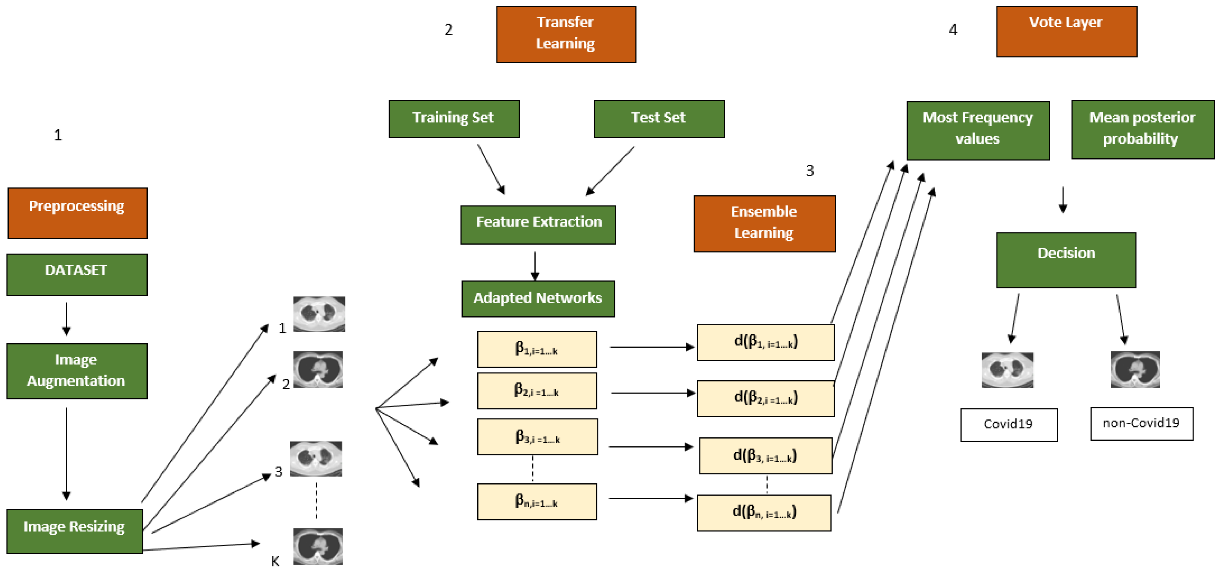
The first level performs preprocessing in terms of image resizing and augmentation. The second learns different deep neural networks, previously redesigned for the specific task. The third combines different models provided by deep neural networks through ensemble rules, for classification. Finally, the framework iterates through a predetermined number of times in a supervised learning context. Figure 1 shows an overview of the proposed framework.

3.1. Image Augmentation

Many approaches have been developed to address the complications associated with the limited amount of data in machine learning. Image augmentation [16] is a functional technique for increasing and/or changing the size of the training set without acquiring additional images. The concept is basic and consists of duplicating and/or modifying the images with some kind of variation so that more samples can help to train the model.

As general idea, the image is augmented in a way that preserves key features for making predictions but reworked so that the pixels present some form of noise. The augmentation will be harmful if it produces images that are very dissimilar to those used to test the model; therefore, it is clear that this process must be organized in detail. In the proposed framework, we have adopted random reflection, translation, and scaling in order to enhance and augment the image content. As described in the experimental section, this step turns out to be fundamental in improving the performance of the proposed approach.

3.2. Image Resize

One of the defects of neural networks concerns the fixed size of the images to be processed. To this end, a resize step is performed based on the input layer dimension claimed by the deep neural networks (details can be found in

Table 1. Description of the adopted pretrained network.

Network	Depth	Size (MB)	Parameters (Millions)	Input Size
Resnet18	18	44	11.7	224 × 224
Densenet201	201	77	20.0	224 × 224
Mobilenetv2	53	13	3.5	224 × 224
Shufflenet	50	6.3	1.4	224 × 224

column 5). Most of the networks require this trick but it does not alter the image information content in any way. The size normalization is essential because images of different or large dimensions cannot be processed for the network training and classification stages.

3.3. Network Design and Transfer Learning

The transfer learning approach was selected for classification. The basic idea is to transfer the knowledge extracted from a source domain to a destination one—in our case, the COVID-19 diagnosis. Generally, a pretrained network is chosen as starting point in order to learn a new task. It is the easiest and fastest solution to adopt the representational power of pretrained deep networks.

Clearly, it is much faster and easier to tune a network with transfer learning rather than training a new network from scratch with randomly initialized weights. For a COVID-19 diagnosis, deep learning architectures were selected based on their structure and performance skills. The goal was to train networks on images by redesigning their structures in the final layer according to the needs of the addressed task (two outgoing classes: COVID-19 and non-COVID-19). Table 1 supports the below description of adopted networks.

Resnet18 [17] is inspired by pyramidal cells contained in the cerebral cortex. It uses particular skip connections or shortcuts to jump over some layers. It is composed of 18 layers, which, with the help of a technique known as a skip connection, has paved the way for residual networks.

Densenet201 [18] is a convolutional neural network that is 201 layers deep. Unlike standard convolutional networks composed of L layers with L one-to-one connections between the current layers and the next, it contains $\frac{L(L+1)}{2}$ direct connections. Specifically, each layer adopts the feature-maps of all preceding layers and its own feature-maps into all subsequent layers as inputs.

Mobilenetv2 [19] is a convolutional neural network that is 53 layers deep. It was built based on an inverted residual structure with shortcut connections between the thin bottleneck layers. The intermediate expansion layer uses lightweight depthwise convolutions to filter features as a source of non-linearity. Furthermore, non-linearities in the narrow layers are removed with purpose to maintain representational power.

Shufflenet [20] is a convolutional neural network with 173 layers designed for mobile devices with very limited computing power. The peculiarity of this architecture concerns the introduction of pointwise group convolution and channel shuffle operations in order reduce computation costs and maintain accuracy.

Deep neural networks have been adapted to the COVID-19 classification problem. Originally, the main training phase was performed on the Imagenet dataset [21], which includes a million images divided into 1000 classes. The results consist of a rich features representation for a wide range of images. The network processes an image and provides a prediction about a class to which it could belong with an attached probability. Commonly, the first layer of the network is the image input layer. The input requires images with three color channels. Immediately after, this is followed by convolutional layers, which work with purpose to extract image features.

Particularly, the last learnable layer and the final classification layer are adopted to classify the input image. In order to make the pretrained network compliant to classify new images, the two last layers with new layers are replaced. Frequently, the last layer, with related learnable weights, is fully connected. This layer is removed and replaced by a new layer that is fully connected with the outputs related to number of classes of new data (COVID-19 and non-COVID-19).

In addition, the learning phase of the new layer, compared to the transferred layers, can be sped up by increasing the rate factors. Optionally, the weights of previous levels can be left unchanged by setting their learning rate to zero. This variation prevents updating of the weights during training, and a consequent lowering of the execution time as the gradients of the relative layers do not have to be calculated. This aspect has a strong impact in the case of small datasets in order to avoid overfitting.

3.4. Ensemble Learning

The contribution of different deep neural networks can be mixed in an ensemble context. Considering the set, with cardinality k, of images belonging to x classes (COVID-19 and non-COVID-19), to be classified

$$Imgs=\{i_1,i_2,\dots ,i_k\}$$

(1)

each image of the set will be treated with the procedure below. Let us consider the set C composed of n deep neural networks

$$C=\{{\beta }_1,{\beta }_2,\dots ,{\beta }_n\}$$

(2)

the images are subjected to the analysis of each deep neural network, thus, generating the set $CN$

$$CN=\left[\begin{array}{ccc}{\beta }_1{i}_1& \cdots & {\beta }_1{i}_k\\ ⋮& \ddots & \\ {\beta }_n{i}_1& & {\beta }_n{i}_k\end{array}\right]$$

(3)

each deep neural network ${\beta }_n$ provides a decision $d\in \{-1,1\}$, regarding classification, where 1 stands for non-COVID and $-1$ for COVID, with reference to each $i_k\in Imgs$. The set of decisions D can be collected as follows

$$D=\left[\begin{array}{ccc}{d}_{{\beta }_1{i}_1}& \cdots & d_{{\beta }_1{i}_k}\\ ⋮& \ddots & \\ d_{{\beta }_n{i}_1}& & d_{{\beta }_n{i}_k}\end{array}\right]$$

(4)

it should be noted that each element of the matrix D corresponds to the result of the deep neural network and image combination of the $CN$ in terms of position within the matrix, such as ${\beta }_n{i}_k\to d_{{\beta }_n{i}_k}$. Furthermore, a score value s, $s\in \{0,\cdots ,1\}$, is associated with each decision d and represents the posterior probability $P\left(i\right|x)$ that an image i could belong to class x. In addition, the set of scores S can be defined as follows

$$S=\left[\begin{array}{ccc}P{\left(i_1\right|x)}_{d_{{\beta }_1{i}_1}}& \cdots & P{\left(i_k\right|x)}_{d_{{\beta }_1{i}_k}}\\ ⋮& \ddots & \\ P{\left(i_1\right|x)}_{d_{{\beta }_n{i}_1}}& & P{\left(i_k\right|x)}_{d_{{\beta }_n{i}_k}}\end{array}\right].$$

(5)

In this case, each element of the matrix S corresponds to the results of the deep neural network and image combination of $CN$ with related posterior probability in terms of position within the matrix, such as ${\beta }_n{i}_k\to d_{{\beta }_n{i}_k}\to P{\left(i_k\right|x)}_{d_{{\beta }_n{i}_k}}$. At this point, let us introduce the concept of mode, defined as the value that repeatedly occurs in a given set

$$mode=l+\left(\frac{f_1-f_0}{2f_1-f_0-f_2}\right)\times h$$

(6)

where l is the lower limit of the modal class, h is the size of the class interval, $f_1$ is the frequency of the modal class, $f_0$ is the frequency of the class that precedes the modal class, and $f_2$ is the frequency of the class that follows the modal class. In order to obtain the values of the most frequent decisions, each column of the matrix D is analyzed through the mode. This step is performed with purpose to to verify the best responses of the different deep neural networks, contained in the set C. Moreover, the meaning of the mode is twofold. First, it is the most frequent value. Second, its occurrences are in terms of indices. For each modal value, the most frequent occurrence, i.e., the corresponding score from the matrix S is extracted. In this regard, the vector $DS$ is generated

$$DS=\{d{s}_{P{\left(i_1\right|x)}_{d_{{\beta }_{1,\cdots ,n}{i}_1}}},\dots ,d{s}_{P{\left(i_k\right|x)}_{d_{{\beta }_{1,\cdots ,n}{i}_k}}}\},$$

(7)

where each element $ds$ contains the average of the decision scores of modal value with reference to the related column of the matrix D. The modal value of each column of the matrix D is stored in the vector $DM$

$$DM=\{d{m}_{d_{{\beta }_{1,\cdots ,n}{i}_1}},\cdots ,d{m}_{d_{{\beta }_{1,\cdots ,n}{i}_k}}\},$$

(8)

each value $dm$ contains the modal value of the class to which image i could belong with the average probability score $ds$, such as $d{s}_{P{\left(i_k\right|x)}_{d_{{\beta }_{1,\cdots ,n}{i}_k}}}\to d{m}_{d_{{\beta }_{1,\cdots ,n}{i}_k}}$. In essence, this is the class to which an image could belong based on the votes given by different deep neural networks.

4. Experimental Results

This section describes the experiments performed on the public dataset. In order to produce compliant performance, the settings reported in recent COVID-19 classification methods were adopted. The experimental phase was structured in two parts with the purpose to address the COVID-19 detection task. The first concerns a comparison with deep neural networks, in order to prove how a multiple model can provide better guidance compared with a single. The second deals with recent methods, which adopt a different logic than the proposed approach.

4.1. Dataset

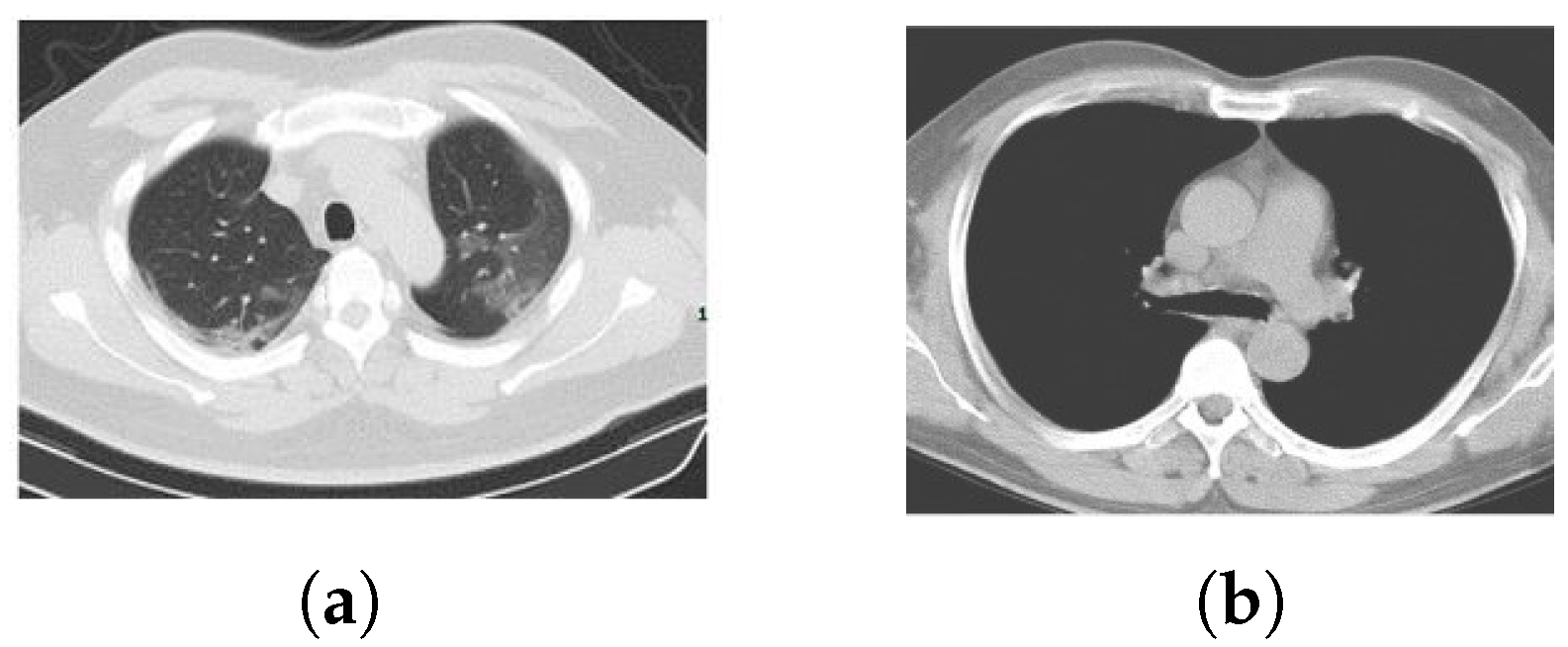
The COVID-19 CT adopted dataset is publicly available (https://github.com/UCSD-AI4H/COVID-CT) and the details are described in [22]. It is composed of 746 Thorax Computer Tomography (CT) images, where 349 contain clinical findings of COVID-19 from 216 patients and 397 are obtained from non-COVID-19 patients. The CT images are a collection selected from COVID-19-related papers published in medRxiv, bioRxiv, NEJM, JAMA, Lancet, and others. The reliability of this dataset has been validated by a senior radiologist, of Tongji Hospital, Wuhan, China, that worked on the diagnosis and treatment of a large number of COVID-19 patients during the period of maximum emergency between January and April 2020. Figure 2 provides some examples of CT images.

4.2. Settings

The framework consists of different modules written in MATLAB language and extends the code available in [23]. The pretrained networks were taken from ImageNet Large-Scale Visual Recognition Challenge (ILSVRC) [24]. Various combinations of networks were selected because the test phase was split by application and not image augmentation. The choice was not random but was made based on the single network performance and an in-depth analysis of their architecture (the number of layers, applications in literature, etc.). A different combination did not provide the expected feedback. Densenet201, Mobilenetv2, and Resnet18 were adopted with image augmentation, while Shufflenet, Resnet18, and Mobilenetv2 were adopted without image augmentation.

Table 1 shows some important details related to the adopted networks. Among all the computational stages, the training process was certainly the most expensive. As is certainly known, the networks are composed of fully connected layers that make the structures extremely dense and complex. This aspect certainly increases the computational load.

In order to compare the results with those obtained in [23], the networks were trained by setting the mini batch size to 5, the maximum epochs to 6, initial learning rate to $3\times {10}^{-4}$ (constant for the training stage), momentum value to $0.9$, gradient threshold method to the L2 norm, factor for L2 regularization (weight decay) to $1\times {10}^{-4}$, and minimum batch size to 10, and the optimizer was a stochastic gradient descent with the momentum (SGDM) algorithm. We randomly included $80\%$ and $20\%$ of the images in the training and testing sets, respectively, for a number of iterations equal to 5 with the aim to calculate the relevant feedback measures reported in

Table 2. Evaluation metrics adopted during the relevance feedback stage.

Metric	Equation
Sensitivity	$\frac{TP}{TP+FN}$
Specificity	$\frac{TN}{TN+FP}$
Accuracy	$\frac{TP+FN}{TP+FP+TN+FN}$
$F_1$	$\frac{2·TP}{2·TP+FP+FN}$

. For each training and before each network validation epoch, the data were shuffled.

The images were converted into RGB space and resized to align with the input format of each pretrained network. The training was performed with and without image augmentation. Random reflection, translation and scaling were performed for the option of image augmentation. For random reflection, each image was reflected vertically with a probability equal to $0.5$ in the top-bottom direction. Again, a horizontal and vertical translation to each image was applied. The translation distance was selected randomly from a continuous uniform distribution within the specified range $[-30,30]$. Similarly, the images were scaled vertically and horizontally by selecting, in a random way, the scale factor from a continuous uniform distribution within the specified range $[0.9,1.1]$.

4.3. Relevance Feedback

Table 2 summarizes the metrics adopted for the performance evaluation. The goal is to provide a uniform comparison with approaches working on the same task and to understand, from the experimental phase, what information can be useful for a COVID-19 diagnosis.

In order to clarify the understanding of the two classes to be considered, we fixed COVID-19 as a positive class and non-COVID-19 as a negative class. The Sensitivity, also known as the True Positive rate, concerns the portion of images containing COVID-19 disease elements that are correctly identified. The measure provides important information because it highlights the skill to detect images containing the disease and contributes to increasing the degree of robustness of the results.

At the same, it is possible to state the Specificity, also known as the True Negative rate, which instead measures the portion of negatives—images not containing COVID-19 disease elements—that have been correctly identified. Differently, the Accuracy, a well-known performance measure, is the proportion of true results (COVID-19 classified as COVID-19 and non-COVID-19 classified as non-COVID-19) among the total number of cases examined.

Our case provides an overall analysis (certainly a rough measurement compared to the previous ones) regarding the skill of a classifier to distinguish an image of a patient infected with COVID-19 from an image of a patient not infected with COVID-19. Furthermore, $F_1$ is defined as the combination of the precision and recall of the model in terms of the harmonic mean. In addition, the AUC was calculated using the trapezoidal integration to estimate the area under the ROC curve and represents the measure of the performance of a classifier.

The ROC is a probability curve built by showing the True Positive rate against the False Positive rate with different threshold values. The AUC value is contained in the range between 0.5 and 1, where the value 0.5 represents the performance of a random classifier and the value 1 indicates a perfect performance. A high AUC value provides positive classification indications.

4.4. Results

Table 3. Classification results with data augmentation.

Network	Accuracy	Sensitivity	Specificity	F${}_1$ Score	AUC
AlexNet	74.50 ± 4.40	70.46 ± 6.37	79.05 ± 8.61	0.75 ± 0.04	0.83 ± 0.04
GoogLeNet	78.97 ± 3.70	75.95 ± 13.69	82.38 ± 10.53	0.79 ± 0.06	0.91 ± 0.04
SqueezeNet	78.52 ± 7.56	91.56 ± 7.63	63.81 ± 23.79	0.82 ± 0.04	0.90 ± 0.01
ShuffleNet	86.13 ± 10.16	83.54 ± 19.89	89.05 ± 5.77	0.86 ± 0.12	0.93 ± 0.06
ResNet-18	90.16 ± 2.36	89.45 ± 7.31	90.95 ± 9.29	0.91 ± 0.02	0.96 ± 0.05
ResNet-50	92.62 ± 4.19	91.14 ± 3.35	94.29 ± 5.15	0.93 ± 0.04	0.98 ± 0.01
ResNet-101	89.71 ± 10.05	82.28 ± 20.09	98.10 ± 2.18	0.89 ± 0.12	0.97 ± 0.03
Xception	85.68 ± 6.76	90.72 ± 4.79	80.00 ± 19.64	0.87 ± 0.05	0.94 ± 0.04
Inception-v3	91.28 ± 8.25	90.30 ± 5.12	92.38 ± 11.98	0.92 ± 0.08	0.97 ± 0.02
Inception-ResNet-v2	86.35 ± 5.71	88.19 ± 6.37	84.29 ± 14.50	0.87 ± 0.05	0.95 ± 0.05
VGG-16	78.52 ± 10.02	74.68 ± 30.14	82.86 ± 15.91	0.76 ± 0.17	0.91 ± 0.04
VGG-19	83.22 ± 5.85	90.72 ± 3.19	74.76 ± 12.96	0.85 ± 0.04	0.90 ± 0.05
DenseNet-201	91.72 ± 6.52	88.61 ± 8.86	95.24 ± 4.36	0.92 ± 0.07	0.97 ± 0.03
MobileNet-v2	87.25 ± 10.46	95.78 ± 2.64	77.62 ± 21.63	0.89 ± 0.08	0.95 ± 0.04
NasNet-Mobile	83.45 ± 7.36	84.81 ± 2.19	81.90 ± 17.46	0.85 ± 0.05	0.94 ± 0.04
NasNet-Large	85.23 ± 8.25	79.32 ± 16.28	91.90 ± 5.77	0.84 ± 0.10	0.93 ± 0.05
Ensemble	96.38 ± 4.31	95.95 ± 4.51	96.86 ± 7.03	0.97 ± 0.04	0.98 ± 0.03

and

Table 4. Classification results without data augmentation.

Network	Accuracy	Sensitivity	Specificity	F${}_1$ Score	AUC
AlexNet	86.85 ± 13.66	80.25 ± 22.49	94.29 ± 4.84	0.85 ± 0.16	0.94 ± 0.04
GoogLeNet	93.83 ± 6.97	96.71 ± 4.06	90.57 ± 10.53	0.94 ± 0.06	0.96 ± 0.04
SqueezeNet	87.52 ± 6.45	86.84 ± 10.11	88.29 ± 12.01	0.88 ± 0.06	0.94 ± 0.06
ShuffleNet	95.97 ± 5.09	95.44 ± 7.47	96.57 ± 2.96	0.96 ± 0.05	0.97 ± 0.03
ResNet-18	95.44 ± 8.02	98.99 ± 1.65	91.43 ± 15.25	0.96 ± 0.07	0.98 ± 0.03
ResNet-50	93.62 ± 6.17	95.57 ± 6.27	91.43 ± 6.06	0.94 ± 0.06	0.98 ± 0.02
ResNet-101	93.29 ± 5.69	96.20 ± 1.79	90.00 ± 10.10	0.94 ± 0.05	0.98 ± 0.02
Xception	91.11 ± 10.14	89.56 ± 12.55	92.86 ± 7.80	0.91 ± 0.10	0.96 ± 0.03
Inception-v3	93.62 ± 5.22	96.20 ± 0.00	90.71 ± 11.11	0.94 ± 0.07	0.97 ± 0.04
Inception-ResNet-v2	88.59 ± 7.59	89.24 ± 2.69	87.86 ± 13.13	0.89 ± 0.07	0.96 ± 0.05
VGG-16	89.26 ± 8.80	92.83 ± 6.24	85.24 ± 14.45	0.90 ± 0.08	0.96 ± 0.03
VGG-19	90.16 ± 7.72	87.34 ± 10.36	93.33 ± 5.77	0.90 ± 0.08	0.97 ± 0.03
DenseNet-201	96.20 ± 4.95	95.78 ± 5.27	96.67 ± 4.59	0.96 ± 0.05	0.98 ± 0.03
MobileNet-v2	95.97 ± 7.18	96.71 ± 6.04	95.14 ± 8.55	0.96 ± 0.07	0.97 ± 0.05
NasNet-Mobile	89.26 ± 8.14	91.56 ± 5.12	86.67 ± 13.27	0.90 ± 0.07	0.95 ± 0.06
NasNet-Large	88.59 ± 7.59	90.51 ± 0.90	86.43 ± 17.17	0.90 ± 0.06	0.96 ± 0.03
Ensemble	96.51 ± 6.34	96.96 ± 4.79	96.00 ± 8.17	0.97 ± 0.06	0.99 ± 0.03

describe the comparison with different deep neural networks applying and not applying image augmentation. The provided performance can be considered satisfactory compared to different neural architectures. In terms of accuracy, although it provides a rough measurement, we have provided the best result with and without image augmentation. The Sensitivity, a measure that provides greater confidence about the addressed problem, is very high for both cases. Otherwise, the Specificity, which also provides a high degree of information related to the absence of COVID-19 within the image, is the best value for both cases.

Regarding the remaining measures, the F${}_1$ score and AUC, considerable values were obtained.

Table 5. Comparison with other methods.

Method	Accuracy
Zhao et al. [7]	78.6
Bernheim et al. [8]	88.0
Gozes et al. [9]	95.0
Zheng et al. [10]	90.1
Ai et al. [11]	97.0
Fang et al. [12]	98.0
(Ctnet-10) [6]	82.1
(VGG-19) [6]	94.5
Ensemble (data augmentation)	96.3
Ensemble (no data augmentation)	96.5

provides comparison results with existing COVID-19 classification methods in terms of accuracy. As shown, our proposed approach was only surpassed by [11,12]. For the remaining methods, the performance provided was better. Data augmentation produces a slight decrease in performance but remains in the same order of magnitude.

The effectiveness of the results can be attributed to two main aspects: deep neural networks and a competitive model for classification. First, the deep neural networks chosen for image learning and classification are the main strong points. Furthermore, the framework provides multiple learning models that certainly constitute a different starting point compared with a standard approach, in which a single model is provided. This aspect is relevant for improving the performance.

Second, the classification stage provides multiple choices in decision making. At each iteration, the framework selects which networks are suitable for recognizing COVID-19 in the images of the test set. Certainly, the computational load is greater but produces better results than a single classification approach. A not negligible issue concerns the image size normalization, with respect to the request of the first layer of the neural networks, before the leaning phase, which does not produce a performance degradation. In other cases, degradation of the image details, quality, and content is due to normalization.

Otherwise, the weak point is the computational load even if the pretrained networks include layers with already tuned weights. The time required for the training stage is long and computational resources are high; however, these are less than with a network created from scratch. Moreover, the addressed binary classification has not been greatly disadvantaged by the problem of class imbalance because the relationship between the number of images per class is not very unbalanced. In many cases, data imbalance impacts a low prediction of accuracy for the minority class.

This is open problem but the solutions are many, such as undersampling the majority class or oversampling the minority classes using image augmentation or a weighted loss method by updating the loss function to result in the same method for all classes. This behavior is often seen in medical data due to the limitations of patient samples and cost of acquiring annotated data. Furthermore, in the case of COVID-19 diagnosis, it could be relevant as data relating to patients are not completely public.

5. Conclusions and Future Works

The challenge in COVID-19 detection is particularly interesting when the data comes from visual information. The complexity of the task is linked to different factors, such as the constant increase and variation of data, given that the challenge is in full swing. In support, the convolutional neural networks provide great help to understand the meaning of the information inside the images with the subsequent goal of their classification. In this context, we proposed a framework that combines convolutional neural networks, adapted to the COVID-19 detection task, through a transfer learning approach, using ensemble criteria.

The results produced certainly support the theoretical thesis. A multiple model, based on different deep neural networks, compared to a single one provides a high discrimination factor. The extensive experimental phase demonstrated how the proposed approach was competitive with, and in some cases surpassed, the state of the art methods. Certainly, the main weak point concerns the computational complexity related to the learning phase, which, as is known, requires a long time especially as the data to be processed grows.

Future works concern many directions. First, the goal includes the study and analysis of convolutional neural networks that are still unexplored for this type of problem. Second is the analysis of the features that the networks create for the diagnosis. Methods, such as SHapley Additive exPlanations (SHAP) [25], could be applied to learn feature importance and explain the model output. Third is the application of the proposed framework to additional datasets [14,15] with the purpose to definitively succeed in the challenge of identifying COVID-19.

References

- Kanji, J.N.; Zelyas, N.; MacDonald, C.; Pabbaraju, K.; Khan, M.N.; Prasad, A.; Hu, J.; Diggle, M.; Berenger, B.M.; Tipples, G. False negative rate of COVID-19 PCR testing: A discordant testing analysis. Virol. J. 2021, 18, 1–6. [Google Scholar] [CrossRef] [PubMed]
- Loey, M.; Manogaran, G.; Khalifa, N.E.M. A deep transfer learning model with classical data augmentation and cgan to detect covid-19 from chest ct radiography digital images. Neural Comput. Appl. 2020, 1–13. [Google Scholar] [CrossRef] [PubMed]
- Amyar, A.; Modzelewski, R.; Li, H.; Ruan, S. Multi-task deep learning based CT imaging analysis for COVID-19 pneumonia: Classification and segmentation. Comput. Biol. Med. 2020, 126, 104037. [Google Scholar] [CrossRef] [PubMed]
- He, X.; Yang, X.; Zhang, S.; Zhao, J.; Zhang, Y.; Xing, E.; Xie, P. Sample-Efficient Deep Learning for COVID-19 Diagnosis Based on CT Scans. medRxiv 2020. [Google Scholar] [CrossRef]
- El-Kenawy, E.S.M.; Ibrahim, A.; Mirjalili, S.; Eid, M.M.; Hussein, S.E. Novel feature selection and voting classifier algorithms for COVID-19 classification in CT images. IEEE Access 2020, 8, 179317–179335. [Google Scholar] [CrossRef]
- Shah, V.; Keniya, R.; Shridharani, A.; Punjabi, M.; Shah, J.; Mehendale, N. Diagnosis of COVID-19 using CT scan images and deep learning techniques. Emerg. Radiol. 2021, 28, 497–505. [Google Scholar] [CrossRef] [PubMed]
- Zhao, W.; Zhong, Z.; Xie, X.; Yu, Q.; Liu, J. Relation between chest CT findings and clinical conditions of coronavirus disease (COVID-19) pneumonia: A multicenter study. Am. J. Roentgenol. 2020, 214, 1072–1077. [Google Scholar] [CrossRef] [PubMed]
- Bernheim, A.; Mei, X.; Huang, M.; Yang, Y.; Fayad, Z.A.; Zhang, N.; Diao, K.; Lin, B.; Zhu, X.; Li, K.; et al. Chest CT findings in coronavirus disease-19 (COVID-19): Relationship to duration of infection. Radiology 2020, 259, 200463. [Google Scholar] [CrossRef] [PubMed] [Green Version]
- Gozes, O.; Frid-Adar, M.; Greenspan, H.; Browning, P.D.; Zhang, H.; Ji, W.; Bernheim, A.; Siegel, E. Rapid ai development cycle for the coronavirus (covid-19) pandemic: Initial results for automated detection & patient monitoring using deep learning ct image analysis. arXiv 2020, arXiv:2003.05037. [Google Scholar]
- Zheng, C.; Deng, X.; Fu, Q.; Zhou, Q.; Feng, J.; Ma, H.; Liu, W.; Wang, X. Deep learning-based detection for COVID-19 from chest CT using weak label. medRxiv 2020. [Google Scholar] [CrossRef] [Green Version]
- Ai, T.; Yang, Z.; Hou, H.; Zhan, C.; Chen, C.; Lv, W.; Tao, Q.; Sun, Z.; Xia, L. Correlation of chest CT and RT-PCR testing in coronavirus disease 2019 (COVID-19) in China: A report of 1014 cases. Radiology 2020, 296, 200642. [Google Scholar] [CrossRef] [PubMed] [Green Version]
- Fang, Y.; Zhang, H.; Xie, J.; Lin, M.; Ying, L.; Pang, P.; Ji, W. Sensitivity of chest CT for COVID-19: Comparison to RT-PCR. Radiology 2020, 296, 200432. [Google Scholar] [CrossRef] [PubMed]
- Giannitto, C.; Sposta, F.M.; Repici, A.; Vatteroni, G.; Casiraghi, E.; Casari, E.; Ferraroli, G.M.; Fugazza, A.; Sandri, M.T.; Chiti, A.; et al. Chest CT in patients with a moderate or high pretest probability of COVID-19 and negative swab. Radiol. Med. 2020, 125, 1260–1270. [Google Scholar] [CrossRef] [PubMed]
- Chatzitofis, A.; Cancian, P.; Gkitsas, V.; Carlucci, A.; Stalidis, P.; Albanis, G.; Karakottas, A.; Semertzidis, T.; Daras, P.; Giannitto, C.; et al. Volume-of-Interest Aware Deep Neural Networks for Rapid Chest CT-Based COVID-19 Patient Risk Assessment. Int. J. Environ. Res. Public Health 2021, 18, 2842. [Google Scholar] [CrossRef] [PubMed]
- Ning, W.; Lei, S.; Yang, J.; Cao, Y.; Jiang, P.; Yang, Q.; Zhang, J.; Wang, X.; Chen, F.; Geng, Z.; et al. Open resource of clinical data from patients with pneumonia for the prediction of COVID-19 outcomes via deep learning. Nat. Biomed. Eng. 2020, 4, 1197–1207. [Google Scholar] [CrossRef] [PubMed]
- Shorten, C.; Khoshgoftaar, T.M. A survey on image data augmentation for deep learning. J. Big Data 2019, 6, 60. [Google Scholar] [CrossRef]
- He, K.; Zhang, X.; Ren, S.; Sun, J. Deep residual learning for image recognition. In Proceedings of the IEEE Conference on Computer Vision and Pattern Recognition, Las Vegas, NV, USA, 27–30 June 2016; pp. 770–778. [Google Scholar]
- Huang, G.; Liu, Z.; Van Der Maaten, L.; Weinberger, K.Q. Densely connected convolutional networks. In Proceedings of the IEEE Conference on Computer Vision and Pattern Recognition, Honolulu, HI, USA, 21–26 July 2017; pp. 4700–4708. [Google Scholar]
- Sandler, M.; Howard, A.; Zhu, M.; Zhmoginov, A.; Chen, L.C. Mobilenetv2: Inverted residuals and linear bottlenecks. In Proceedings of the IEEE Conference on Computer Vision and Pattern Recognition, Salt Lake City, UT, USA, 18–23 June 2018; pp. 4510–4520. [Google Scholar]
- Zhang, X.; Zhou, X.; Lin, M.; Sun, J. Shufflenet: An extremely efficient convolutional neural network for mobile devices. In Proceedings of the IEEE Conference on Computer Vision and Pattern Recognition, Salt Lake City, UT, USA, 18–23 June 2018; pp. 6848–6856. [Google Scholar]
- Deng, J.; Dong, W.; Socher, R.; Li, L.J.; Li, K.; Fei-Fei, L. Imagenet: A large-scale hierarchical image database. In Proceedings of the 2009 IEEE Conference on Computer Vision and Pattern Recognition, Miami, FL, USA, 20–25 June 2009; pp. 248–255. [Google Scholar]
- Zhao, J.; Zhang, Y.; He, X.; Xie, P. COVID-CT-Dataset: A CT scan dataset about COVID-19. arXiv 2020, arXiv:2003.13865. [Google Scholar]
- Pham, T.D. A comprehensive study on classification of COVID-19 on computed tomography with pretrained convolutional neural networks. Sci. Rep. 2020, 10, 1–8. [Google Scholar] [CrossRef] [PubMed]
- Russakovsky, O.; Deng, J.; Su, H.; Krause, J.; Satheesh, S.; Ma, S.; Huang, Z.; Karpathy, A.; Khosla, A.; Bernstein, M.; et al. Imagenet large scale visual recognition challenge. Int. J. Comput. Vis. 2015, 115, 211–252. [Google Scholar] [CrossRef] [Green Version]
- Lundberg, S.M.; Lee, S.I. A Unified Approach to Interpreting Model Predictions. Adv. Neural Inf. Process. Syst. 2017, 30, 4765–4774. [Google Scholar]
Figure 1.
Overview of the proposed framework. The steps of the pipeline are numbered progressively and are accompanied by arrows indicating the data flow analysis. Step 1 indicates image preprocessing as described in Section 3.1 and Section 3.2. Step 2 includes the application of different deep neural networks for the classification task. Step 3 illustrates the ensemble approach as described in Section 3.4. Finally, step 4 shows the vote process for the final decision as described at the end of Section 3.4.
Figure 2.
Dataset CT images: (a) COVID-19, (b) non-COVID-19.