Damage Evaluation of Free-Free Beam Based on Vibration Testing
by
 ,
,
Duong Huong Nguyen
1,2,*, 
Long Viet Ho
1,3,
Thanh Bui-Tien
4,
Guido De Roeck
5 and
Magd Abdel Wahab
1
1
Soete Laboratory, Department of Electrical Energy, Metals, Mechanical Constructions and Systems, Faculty of Engineering and Architecture, Ghent University, 9000 Gent, Belgium
2
Department of Bridge and Tunnel Engineering, Faculty of Bridge and Road, National University of Civil Engineering, Hanoi 100000, Vietnam
3
Department of Bridge and Tunnel Engineering, Faculty of Civil Engineering, University of Transport and Communications Campus in Ho Chi Minh, Ho Chi Minh 700000, Vietnam
4
Department of Bridge and Tunnel Engineering, Faculty of Civil Engineering, University of Transport and Communications, Hanoi 100000, Vietnam
5
Department of Civil Engineering, Structural Mechanics, Katholieke Universiteit Leuven, B-3001 Leuven, Belgium
*
Author to whom correspondence should be addressed.
Appl. Mech. 2020, 1(2), 142-152; https://0-doi-org.brum.beds.ac.uk/10.3390/applmech1020010
Submission received: 25 March 2020
/
Revised: 1 May 2020
/
Accepted: 4 May 2020
/
Published: 9 May 2020
(This article belongs to the Collection Fracture, Fatigue, and Wear)
Abstract
:Damage can be detected by vibration responses of a structure. Damage changes the modal properties such as natural frequencies, mode shapes, and damping ratios. Natural frequency is one of the most frequently used damage indicators. In this paper, the natural frequency is used to monitor damage in a free-free beam. The modal properties of the intact free-free beam are identified based on a setup of 15 accelerometers. A finite element model is used to model the free-free beam. Three models are considered: beam (1D), shell (2D), and solid (3D). The numerical models are updated based on the first five bending natural frequencies. The free-free beam is damaged by a rectangle cut. The experiment is re-setup and the model properties of the damaged beam are re-identified. The cuttings are modeled in the numerical simulations. The first five numerical bending natural frequencies of the damaged beam are compared with the experimental ones. The results showed that the 1D beam element model has the highest errors, while the 2D and 3D models have approximately the same results. Therefore, the 2D representation can be used to model the damaged beam for fast computation.
1. Introduction
Structural health monitoring (SHM) requires techniques that could detect and locate damage in structures. Vibration-based SHM is based on the principle that damage changes the modal properties of the structures [1]. Some modal properties such as natural frequencies, mode shapes, modal curvatures, and damping ratios were used to detect damage [2,3,4,5,6]. Uniaxial/triaxial accelerometers or velocity meters are traditionally used to collect data from the vibrating structures. Analysis of these data provides the modal properties of the structures. Modal analysis is also helpful in model updating problems. Some material and topological uncertain parameters are adjusted to minimize the differences between experimental data and finite element (FE) modal properties. Normally, the finite element model (FEM) is updated using modal properties of the intact structure [7,8]. FEM provides important model information for engineers and helps to reduce the number of experiments. Some recent studies combined the vibration-based method and machine learning algorithm and recognized their effectuation [9,10]. The updated FE model was used to get the training data for the machine learning network. Whether or not this FE model updating could detectably produce the modal characteristic changes of the damaged structure, as well as intact structure, is a challenging question.
Beam is commonly used in the field of mechanical and structural engineering. Beam is a structural element, which is designed to resist bending, widely used in bridges, buildings, rooftops, and so on. The vibration of a beam has been analyzed using both experimental data and numerical models [11,12,13]. Many damage detection methods were used for the beam-like structure [14,15,16]. In this paper, three FE models in ANSYS 17.0 (ANSYS, Inc. Southpointe, 2600 Ansys Drive, Canonsburg, PA 15317, United states)—beam (1D), shell (2D), and solid (3D)—are considered. The natural frequencies of the intact and damaged beams obtained using FEM are compared with experimental ones (Section 2 and Section 3). The conclusion and discussion about these three FE models are presented in Section 4.
2. Steel Beam Experiments
2.1. Experimental Setup
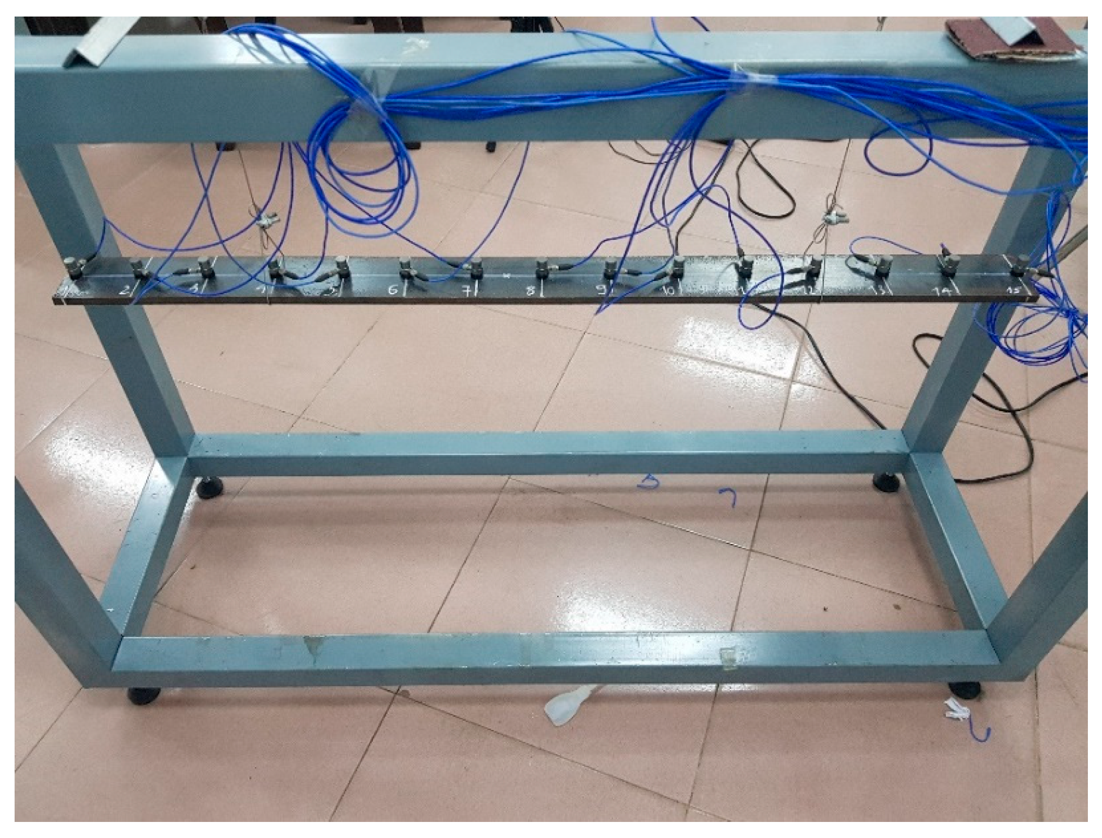
A steel beam, having dimensions of 1 m long × 70 mm wide × 10 mm thick, density of 7820 kg/m3 and the free-free boundary condition, was used for the experiment. The tested beam was suspended by two thin filaments located at the location of accelerometers 4 and 12 to simulate the free-free boundary condition. On the top of the beam, fifteen accelerometers were attached with sensitivity ranges from 10.13 to 10.50 mV/m·s−2. A hammer was used as an excitation force. The tested beam was excited once a time at the location of accelerometer 8 by the hammer. A laptop and National Instruments (NI) equipment were used to record the vibration data. Figure 1 shows the experimental setup in the laboratory and Table 1 shows the location of the accelerometers. The locations in Table 1 are the distance from the accelerometers to the left end of the beam.
2.2. Experimental Results
2.2.1. Intact Beam
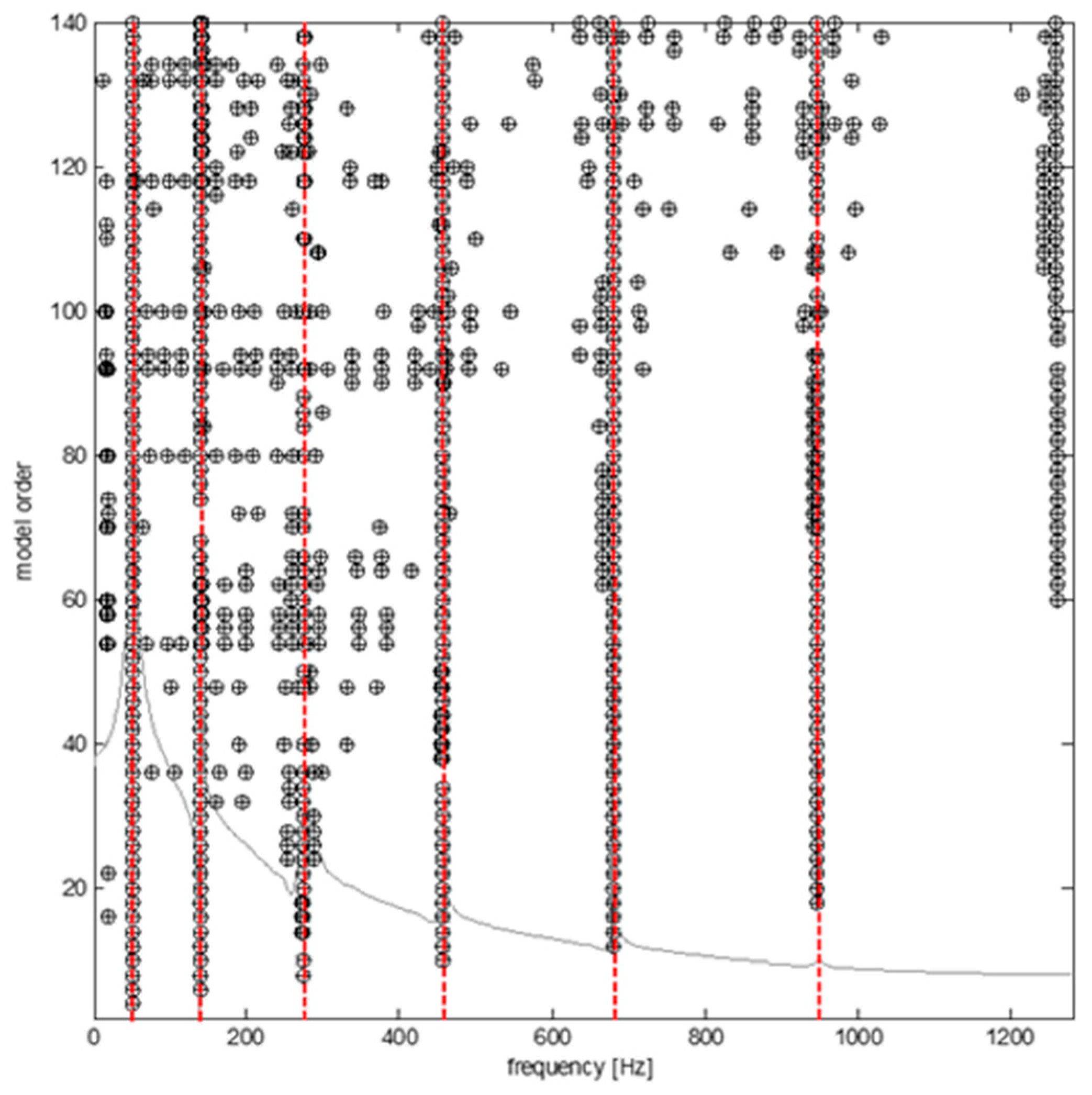
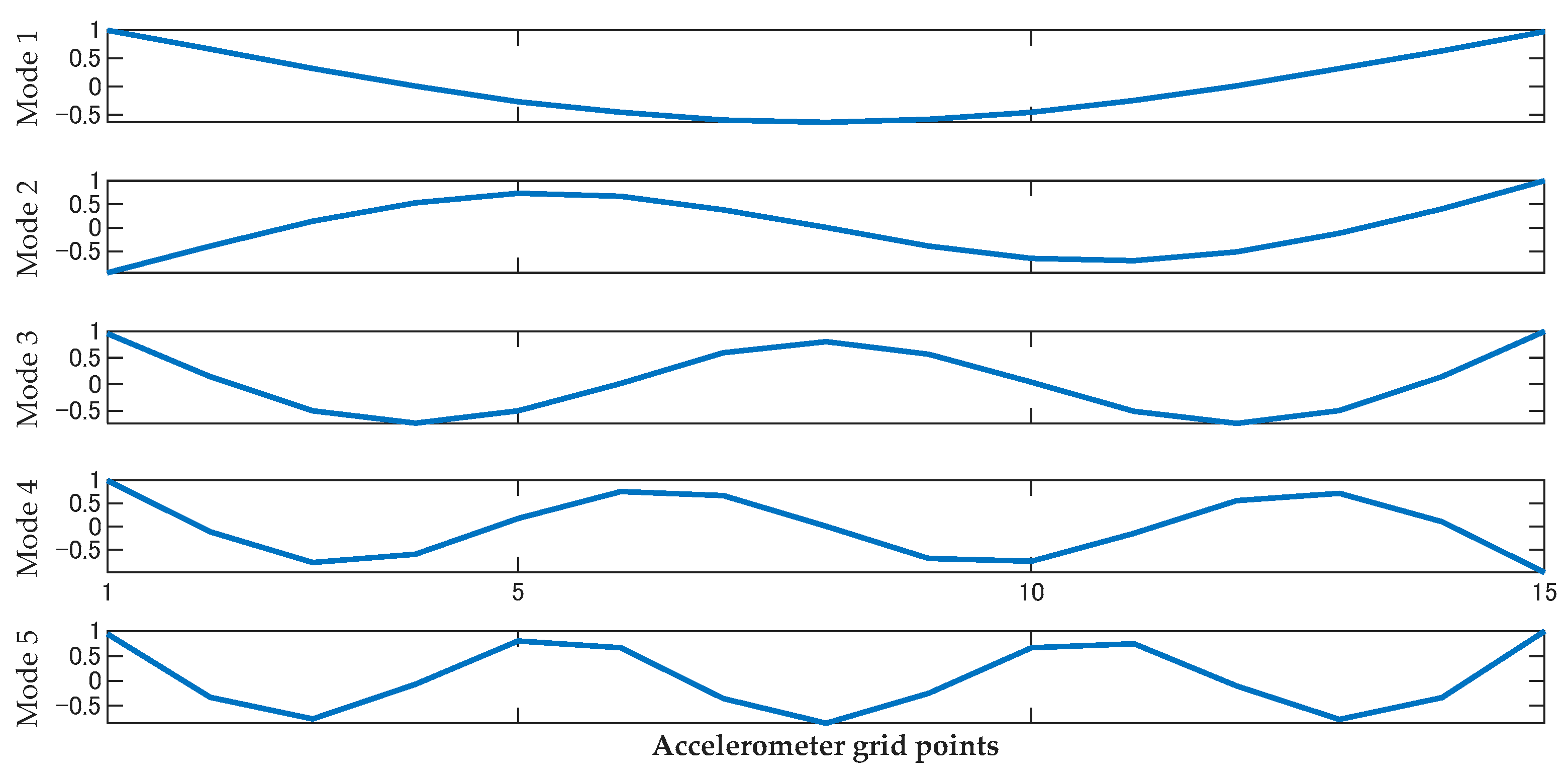
To analyze the collected data, covariance-driven stochastic subspace identification algorithm (SSI-COV) was used thanks to lower time consumption for computation and accuracy [17,18,19]. In general, physical modes and spurious modes are distinguished using a stabilization diagram. A clear stabilization diagram implies that the physical modes are present with consistent modal parameters such as frequencies, damping ratios, and mode shapes. To do that, we compared the poles corresponding to a certain model order to the poles of a one-order lower model. A stable pole is labelled if the differences of frequency, damping ratio, as well as mode shape were within the preset criteria. On the basis of our experience, strictly preset criteria are 1% for frequencies, 5% for damping ratios, and 1% for the mode shape vectors. The stable poles in the stabilization diagram should be selected first (Figure 2). The first five bending modes were identified based on the stabilization diagram, as shown in Figure 3 and presented in Table 2.
2.2.2. Damaged Beam
The beam was damaged by a cutting on the edge. There are two scenarios:
Scenario 1: cut on the left side of the beam, the dimensions of the cutting are 0.5 × 12.5 (mm).
Scenario 2: cut on both sides of the beam, the dimensions of the cutting are 0.5 × 12.5 (mm) and 0.5 × 13.3 (mm).
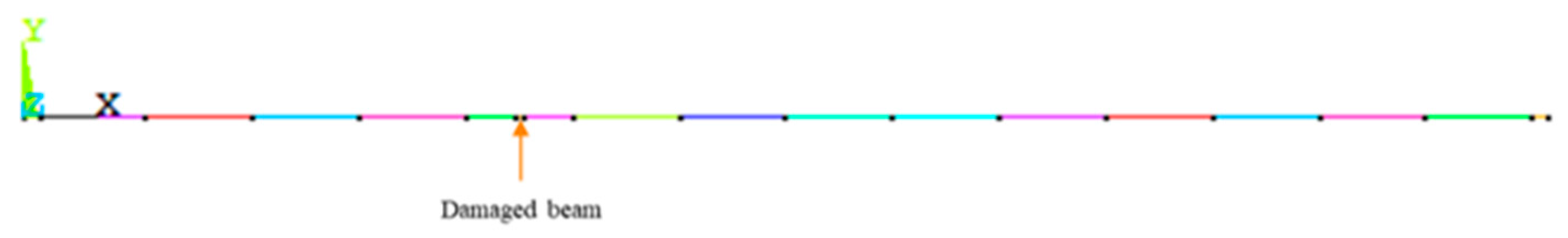
The location of the damage is between accelerometer 5 and 6, as shown in Figure 4.
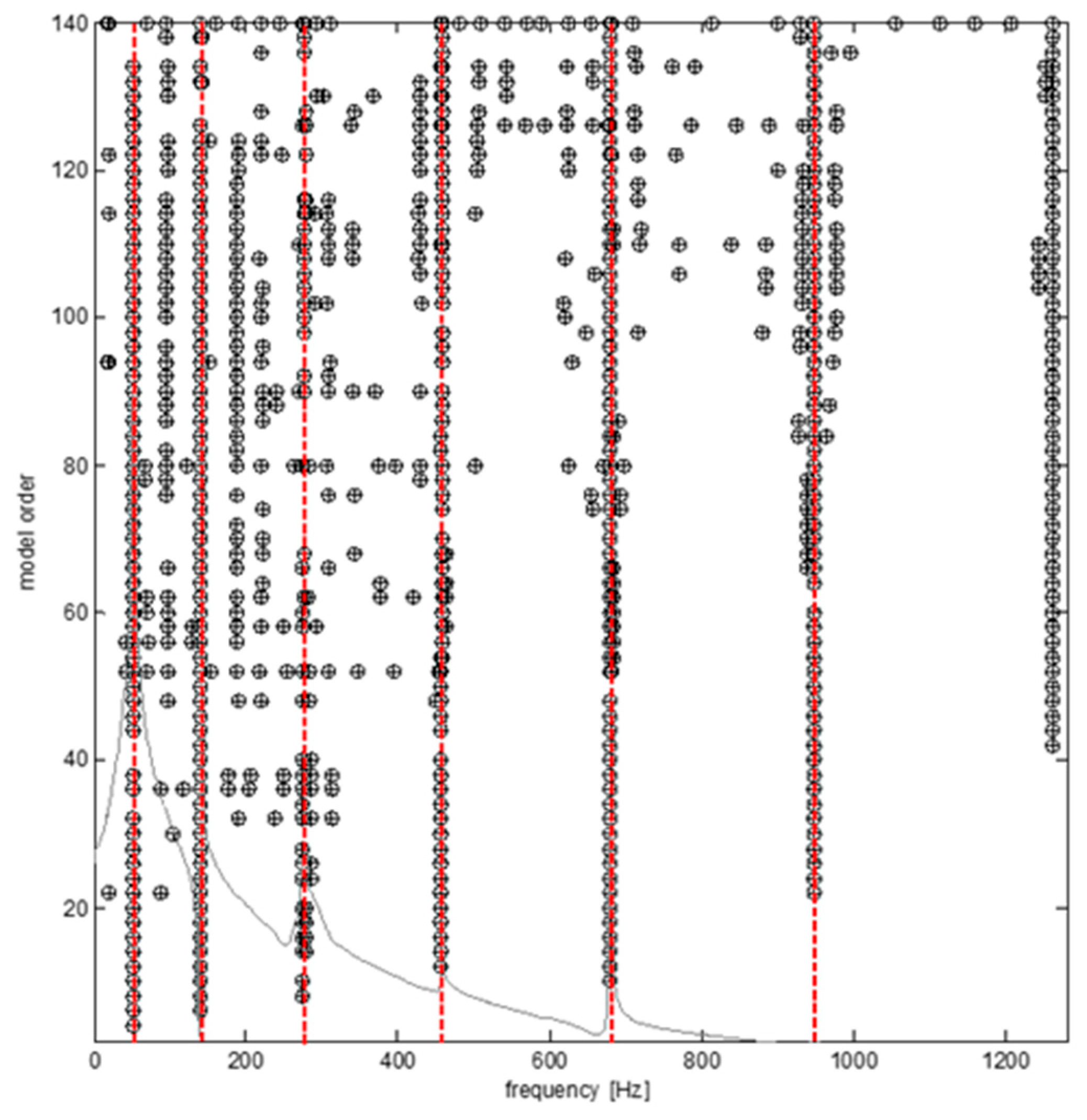
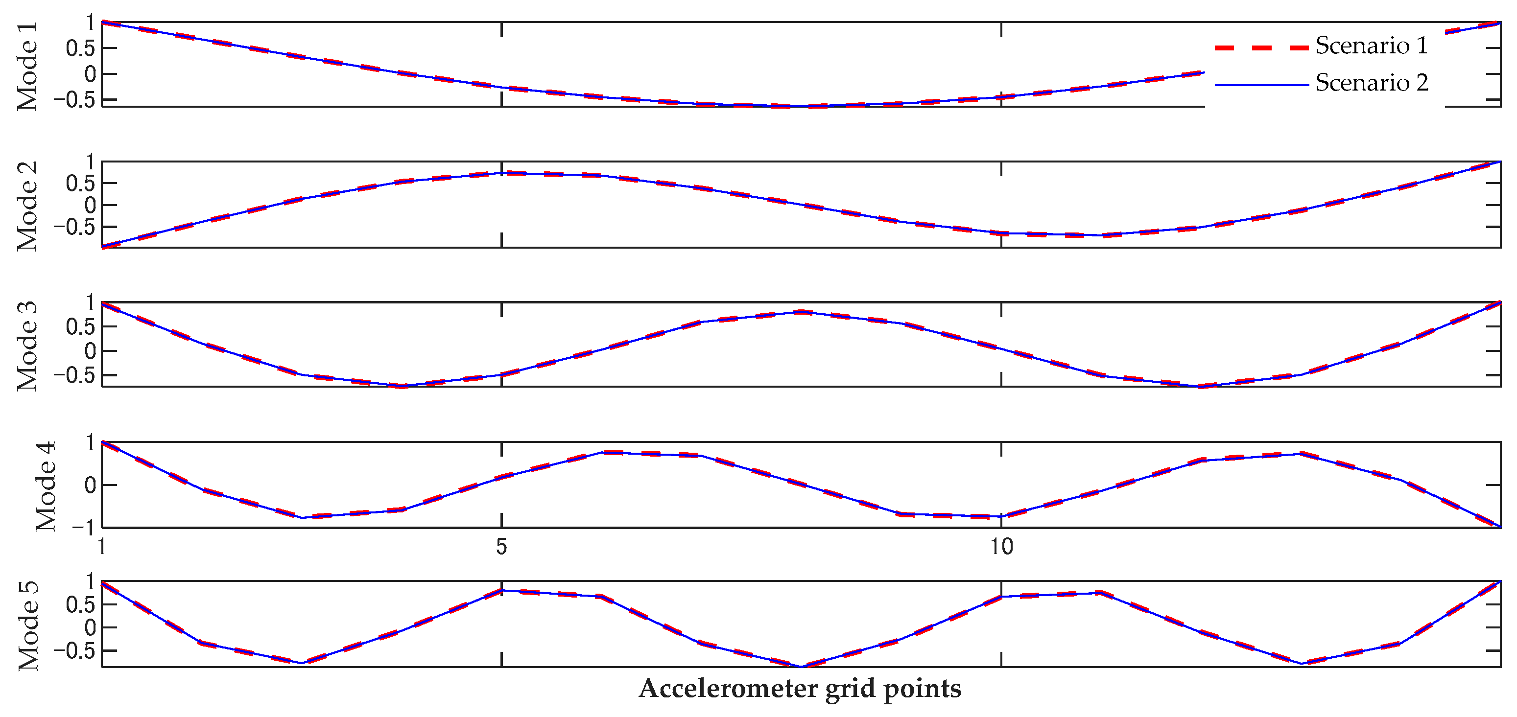
The vibration data were analyzed using the same method as the data from the intact beam. Figure 5 illustrates the stabilization diagram, Figure 6 plots the mode shapes, and Table 3 presents the natural frequencies. From Figure 6 we can see that the mode shapes of the two damaged scenarios are almost the same, whereas the frequencies show a small difference between the intact beam and the two damaged beams.
3. Numerical Models
The free-free beam structure having dimensions of was modeled in ANSYS 17.0. The steel density is ρ , and Young’s modulus .
Three types of elements, that is, beam, shell, and solid elements, were employed to construct the FE models for modal analysis of the free-free beam. The intact beam and two damaged scenarios were considered.
3.1. Beam Model (1D Model)
The steel beam was modeled using BEAM189 in ANSYS 17.0. It is a quadratic beam element in which each node has six degrees of freedom (DOF), that is, three translations and three rotations. The intact beam was modeled by several beam elements with a rectangular cross section of . The number of elements increased until converged results were obtained.
For the damaged beam, the damaged elements were modeled by a reduced width of the cross section. The dimensions of the cross section are and mm for Scenario 1 and Scenario 2, respectively. The models of the intact and damaged beam are illustrated in Figure 7.
3.2. Shell Model (2D Model)
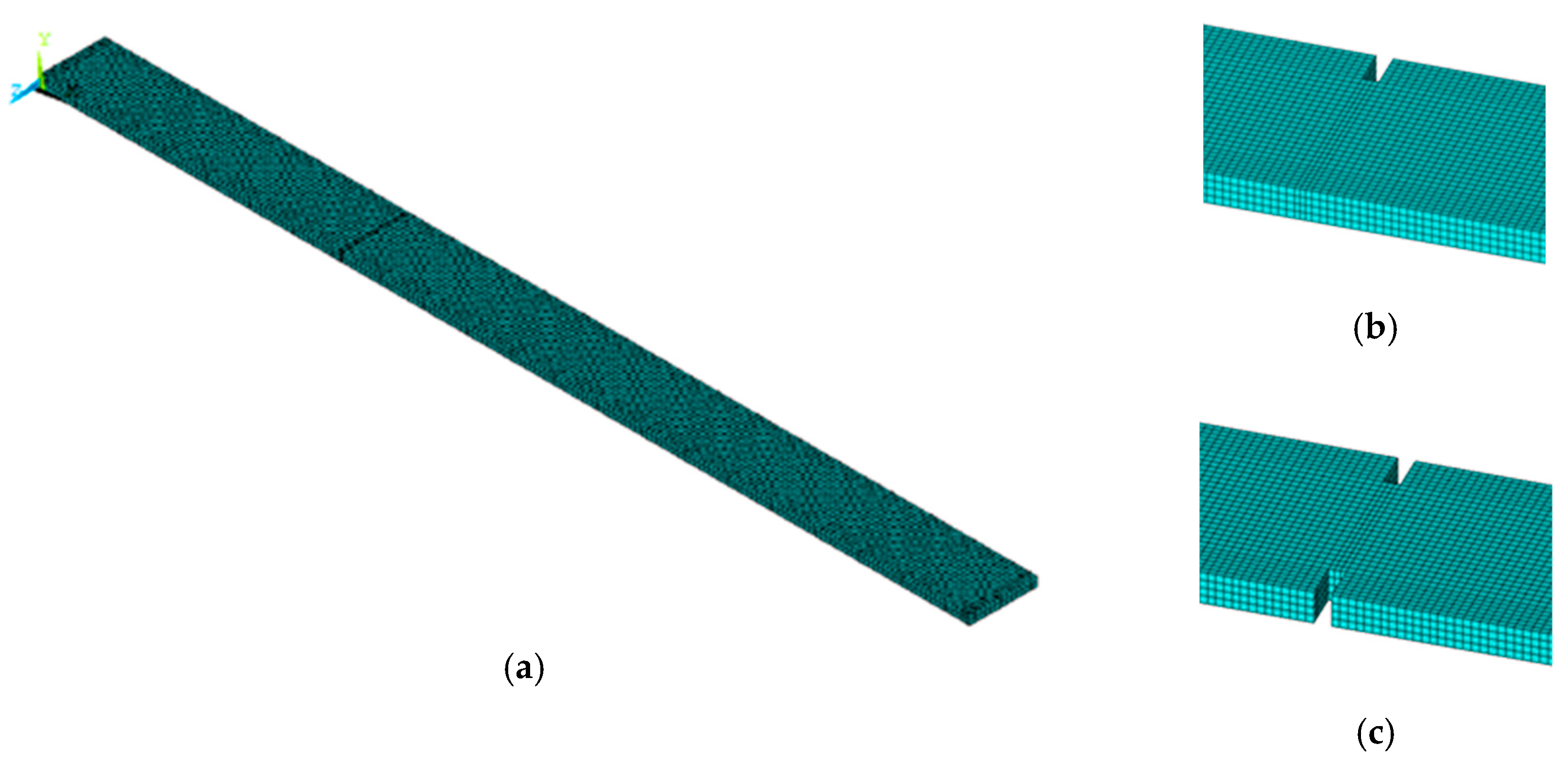
A four-node element, SHELL181, was the next element used to identify the vibration of the beam. This element is suitable for analyzing moderately-thick shell structures as the beam in our study. It has six DOF at each node: three translations in the x, y, and z directions, and three rotations about the x, y, and z axes. Dimensions in the shell model are the same as in the beam model, as mentioned above. The thickness of the surface is defined as 10 mm, whereas the width of the surface is 70 mm. The mesh structure and the FE model of this beam and the numerical models of the two damaged scenarios are shown in Figure 8.
3.3. Solid Model (3D Model)
For further modal analysis, a solid model was built with SOLID185. This type of element is often used for 3D modeling of solid structures. The element is defined by eight nodes with three translations at each node. Figure 9 shows the beam model using a solid element with grid meshing.
4. Results and Discussion
The results from the experiments showed that, when the damage occurs, the natural frequencies of the beam reduced, whereas the change in mode shapes could not be realized directly. Therefore, only natural frequencies are used for a discussion in this section.
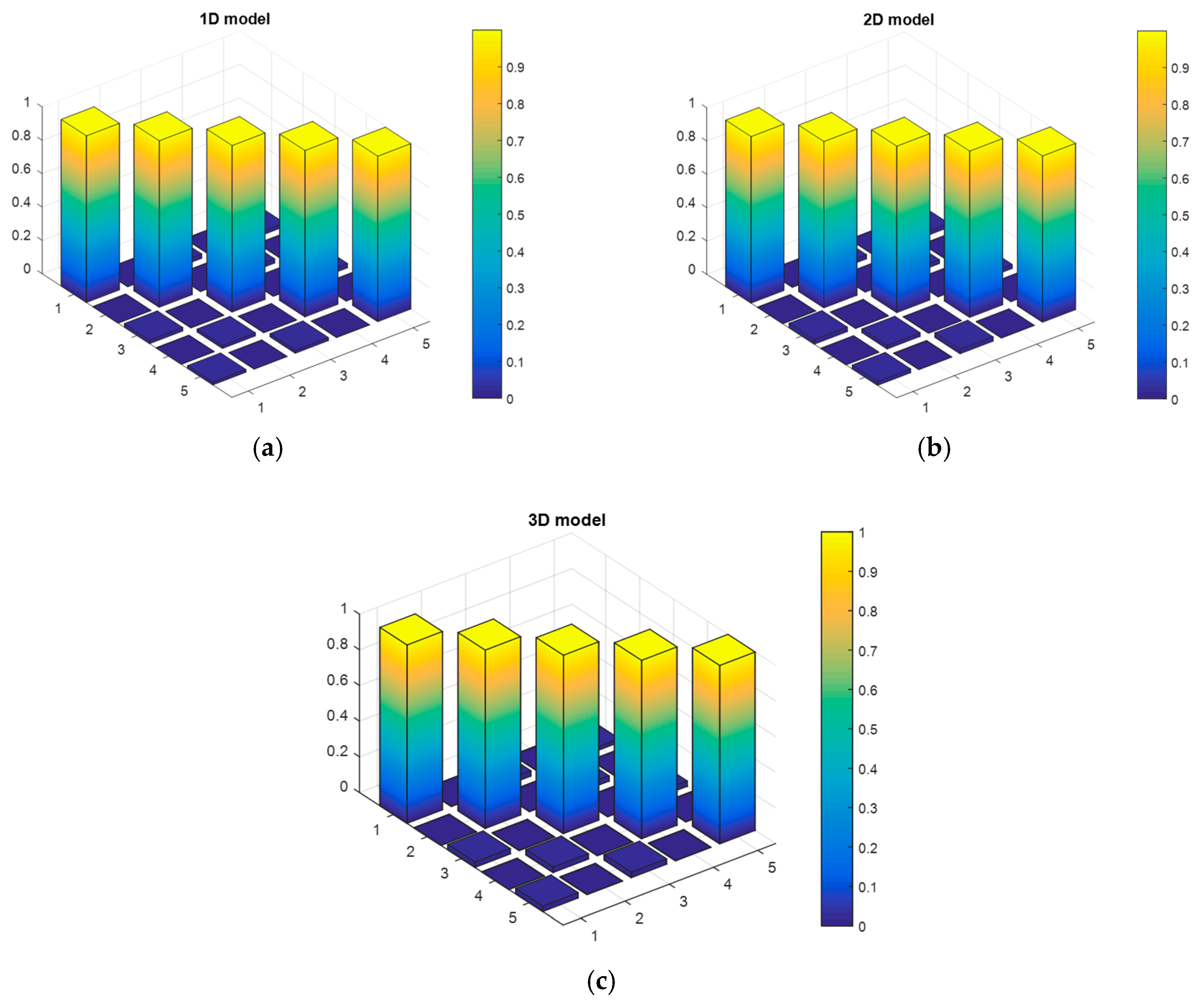
There are small differences between frequencies calculated from the measurements and from the FEM (less than 1.5%). Additionally, correlation between experimental and simulated mode shapes were investigated using the Modal Assurance Criterion (MAC) matrix [20]. MAC values in Figure 10 show a good match between simulation and experiment owing to the average values of MAC being over 0.99 and close to 1.
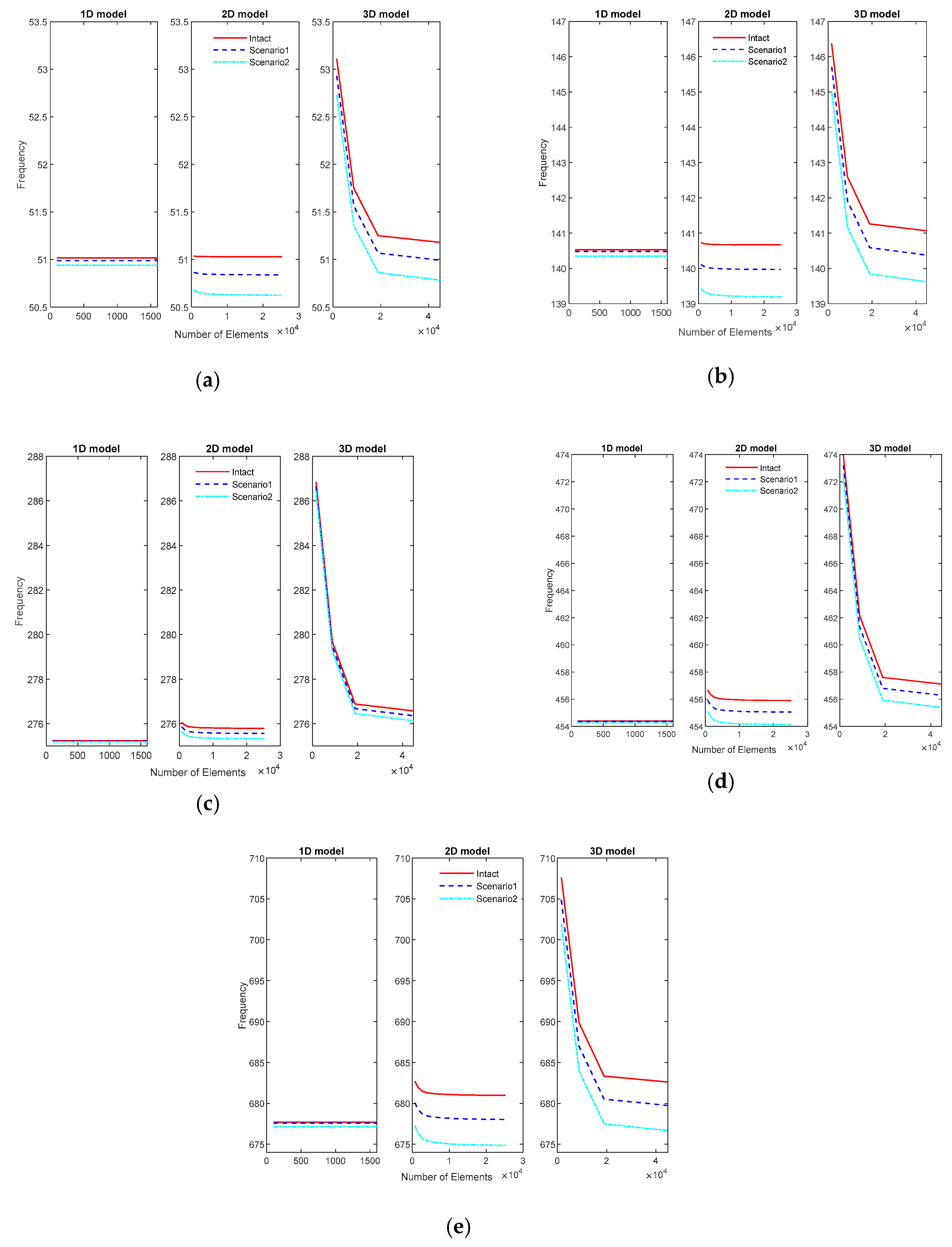
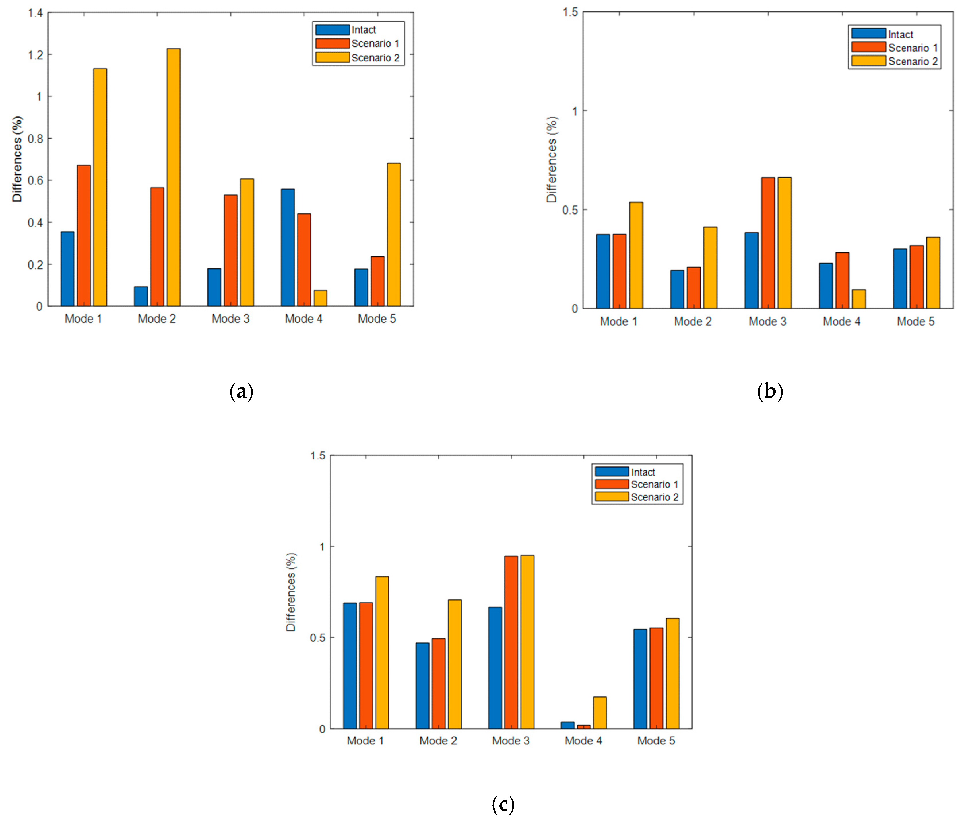
For the numerical models, the number of elements in each model affects the natural frequencies. Figure 11 illustrates the frequencies extracted from the three FE models for the first five modes. The natural frequencies converge when the number of elements in the numerical model increases. Moreover, the 1D model uses a smaller number of elements than the 2D model. The convergence curve of frequency from the 1D model is approximately a line, whereas the 2D model needs more than 1000 elements and the 3D model needs more than 2000 elements to converge. Moreover, one beam element has two nodes, one shell element is presented by four nodes, and one solid element is modeled by eight nodes. Therefore, the computation time for the 3D model is the longest. The converged natural frequencies extracted from the FE model are presented in Table 4 (intact beam), Table 5 (Scenario 1), and Table 6 (Scenario 2). The differences between FEM and experimental data are then calculated and plotted in Figure 12. These are less than 1% in all cases; that is, the FEM can reflect the behavior of the experimental beam.
Observing Figure 12, although the differences in frequencies of the 1D model for the intact beam are the smallest compared with the other models, it increases steadily for the damaged beam. The greater the severity of the damage, the higher the differences between numerical and experimental results. For example, at mode 1, the differences are 0.35%, 0.67%, and 1.13% for intact, damaged beam Scenario 1, and damaged beam Scenario 2, respectively. We can obtain the same results for modes 2, 3, and 5. In the case of the beam having damaged elements, the 1D model could not reflect the vibration response of the damaged beam, and the differences between FEM and experiment are high. The reason would be that there is a force flow around the artificial cuts, which makes parts of the material adjacent to the damage less (shadow zone) and more stressed, which cannot be modeled by beams (except if an effective width is used).
The differences in natural frequencies between the 2D model or 3D model and experiment do not change much for intact, Scenario 1, and Scenario 2. For example, in mode 1 of the 2D model, the differences are 0.35%, 0.375%, and 0.53% for intact, Scenario 1, and Scenario 2, respectively. For mode 1 calculated from the 3D model, these differences are 0.68%, 0.69%, and 0.83% for intact, Scenario 1, and Scenario 2, respectively. This trend is repeated for all five modes. It should be noted that because the cut is near a node of mode 4, the behavior of mode 4 is different than other modes. The severity of damage did not highly affect the accuracy of the 2D model and 3D model. Moreover, the differences between the 2D model and the experimental results are less than those from the 3D model. One thing that must be noticed is that the same material properties were used for both models. These material properties need to be updated for each model to get the best results.
Each element behaves as a plate in the 2D model, and as a solid in the 3D model. Therefore, the time used for computing the 3D model is much longer than that for the 2D model. From the discussion above, we conclude that the 2D model should be used for the damaged beam for simplicity and fast computation.
5. Conclusions
In this paper, a free-free beam was modeled using three kinds of finite elements: beam (1D), shell (2D), and solid (3D). Using the same material properties, each FE model provided different results of natural frequencies. The experiment is conducted in the laboratory using a steel beam. Fifteen accelerometers were set up to measure the first five bending natural frequencies of the beam in free-free position. Three states of the beam were considered: intact beam, and two scenarios of artificial damage. The conclusion was made based on the differences between the numerical models and the experiment of each state. For the 1D model, these differences increase steadily when the severity of the damage increases, whereas the 2D and 3D models have the same trend of changing. Therefore, the 2D model is proposed as the most suitable model of the free-free beam because it is a simple model and runs much faster than the 3D model.
Author Contributions
Methodology, writing—original draft preparation, D.H.N.; software, L.V.H; experimental work, D.H.N. and L.V.H.; validation, T.B.-T.; supervision, G.D.R. and M.A.W. All authors have read and agreed to the published version of the manuscript.
Funding
This research is funded by National University of Civil Engineering (NUCE) under grant number 11-2020/KHXD-TĐ. The authors acknowledge the financial support of VLIR-UOS TEAM Project, VN2018-TEA479A103, ‘Damage assessment tools for Structural Health Monitoring of Vietnamese infrastructures’ funded by the Flemish Government.
Conflicts of Interest
The authors declare no conflict of interest.
References
- Carden, E.P.; Fanning, P. Vibration based condition monitoring: A review. Struct. Health Monit. 2004, 3, 355–377. [Google Scholar] [CrossRef]
- Maia, N.; Silva, J.; Almas, E.; Sampaio, R. Damage detection in structures: From mode shape to frequency response function methods. Mech. Syst. Signal Process. 2003, 17, 489–498. [Google Scholar] [CrossRef]
- Yan, Y.; Cheng, L.; Wu, Z.; Yam, L. Development in vibration-based structural damage detection technique. Mech. Syst. Signal Process. 2007, 21, 2198–2211. [Google Scholar] [CrossRef]
- Thyagarajan, S.; Schulz, M.; Pai, P.; Chung, J. Detecting structural damage using frequency response functions. J. Sound Vib. 1998, 210, 162–170. [Google Scholar] [CrossRef]
- Wahab, M.A.; De Roeck, G. Damage detection in bridges using modal curvatures: Application to a real damage scenario. J. Sound Vib. 1999, 226, 217–235. [Google Scholar] [CrossRef]
- Khatir, S.; Wahab, M.A.; Boutchicha, D.; Khatir, T. Structural health monitoring using modal strain energy damage indicator coupled with teaching-learning-based optimization algorithm and isogoemetric analysis. J. Sound Vib. 2019, 448, 230–246. [Google Scholar] [CrossRef]
- Tran-Ngoc, H.; Khatir, S.; De Roeck, G.; Bui-Tien, T.; Nguyen-Ngoc, L.; Abdel Wahab, M. Model updating for Nam O bridge using particle swarm optimization algorithm and genetic algorithm. Sensors 2018, 18, 4131. [Google Scholar] [CrossRef] [PubMed] [Green Version]
- Oh, B.K.; Kim, M.S.; Kim, Y.; Cho, T.; Park, H.S. Model updating technique based on modal participation factors for beam structures. Comput. Aided Civ. Infrastruct. Eng. 2015, 30, 733–747. [Google Scholar] [CrossRef]
- Nguyen, D.H.; Bui, T.T.; De Roeck, G.; Wahab, M.A. Damage detection in Ca-Non Bridge using transmissibility and artificial neural networks. Struct. Eng. Mech. 2019, 71, 175–183. [Google Scholar]
- Yu, Y.; Wang, C.; Gu, X.; Li, J. A novel deep learning-based method for damage identification of smart building structures. Struct. Health Monit. 2019, 18, 143–163. [Google Scholar] [CrossRef] [Green Version]
- Mahmoud, A.; Abdelghany, S.; Ewis, K. Free vibration of uniform and non-uniform Euler beams using the differential transformation method. Asian J. Math. Appl. 2013, 2013, 1–16. [Google Scholar]
- Orzechowski, G. Analysis of beam elements of circular cross section using the absolute nodal coordinate formulation. Arch. Mech. Eng. 2012, 59, 283–296. [Google Scholar] [CrossRef] [Green Version]
- Li, Q. A new exact approach for determining natural frequencies and mode shapes of non-uniform shear beams with arbitrary distribution of mass or stiffness. Int. J. Solids Struct. 2000, 37, 5123–5141. [Google Scholar] [CrossRef]
- Nguyen, H.D.; Bui, T.T.; De Roeck, G.; Wahab, M.A. Damage Detection in Simply Supported Beam Using Transmissibility and Auto-Associative Neural Network. In International Conference on Numerical Modelling in Engineering; Springer: Singapore, 2018. [Google Scholar]
- Khatir, S.; Belaidi, I.; Serra, R.; Wahab, M.A.; Khatir, T. Damage detection and localization in composite beam structures based on vibration analysis. Mechanics 2015, 21, 472–479. [Google Scholar] [CrossRef] [Green Version]
- Khatir, S.; Belaidi, I.; Serra, R.; Benaissa, B.; Saada, A.A. Genetic algorithm based objective functions comparative study for damage detection and localization in beam structures. J. Phys. Conf. Ser. 2015, 628, 012035. [Google Scholar] [CrossRef] [Green Version]
- Peeters, B. System Identification and Damage Detection in Civil Engeneering. Ph.D. Thesis, Katholieke Universiteit, Leuven, Belgium, 2000. [Google Scholar]
- Peeters, B.; De Roeck, G. Reference-based stochastic subspace identification for output-only modal analysis. Mech. Syst. Signal Process. 1999, 13, 855–878. [Google Scholar] [CrossRef] [Green Version]
- Reynders, E.; De Roeck, G. Reference-based combined deterministic–stochastic subspace identification for experimental and operational modal analysis. Mech. Syst. Signal Process. 2008, 22, 617–637. [Google Scholar] [CrossRef]
- Pastor, M.; Binda, M.; Harčarik, T. Modal assurance criterion. Procedia Eng. 2012, 48, 543–548. [Google Scholar] [CrossRef]
Figure 1.
Experimental setup.

Figure 2.
Stabilization diagram obtained from the experiment of the intact beam.

Figure 3.
The first five bending mode shapes of the intact beam.

Figure 4.
The cutting places in the damaged beam.

Figure 5.
Stabilization diagram obtained from the experiment of the damaged beam.

Figure 6.
The first five bending mode shapes of the damaged beam.

Figure 7.
The beam element model of the damaged beam.

Figure 8.
The shell element model of the intact and damaged beam: (a) intact beam, (b) damage Scenario 1, and (c) damage Scenario 2.
Figure 8.
The shell element model of the intact and damaged beam: (a) intact beam, (b) damage Scenario 1, and (c) damage Scenario 2.

Figure 9.
The solid element model of the intact and damaged beam: (a) intact beam, (b) damage Scenario 1, and (c) damage Scenario 2.
Figure 9.
The solid element model of the intact and damaged beam: (a) intact beam, (b) damage Scenario 1, and (c) damage Scenario 2.

Figure 10.
MAC values between experimental and simulated mode shapes: (a) 1D model, (b) 2D model, and (c) 3D model.
Figure 10.
MAC values between experimental and simulated mode shapes: (a) 1D model, (b) 2D model, and (c) 3D model.

Figure 11.
The frequencies extracted from the finite element model (FEM): (a) mode 1, (b) mode 2, (c) mode 3, (d) mode 4, and (e) mode 5.
Figure 11.
The frequencies extracted from the finite element model (FEM): (a) mode 1, (b) mode 2, (c) mode 3, (d) mode 4, and (e) mode 5.

Figure 12.
The frequency differences between numerical and experimental results: (a) 1D model, (b) 2D model, and (c) 3D model.
Figure 12.
The frequency differences between numerical and experimental results: (a) 1D model, (b) 2D model, and (c) 3D model.


Table 1.
Accelerometers location.
| Location | 1 | 2 | 3 | 4 | 5 | 6 | 7 | 8 |
|---|---|---|---|---|---|---|---|---|
| Position (m) | 0.01 | 0.08 | 0.15 | 0.22 | 0.29 | 0.36 | 0.43 | 0.5 |
| Location | 9 | 10 | 11 | 12 | 13 | 12 | 15 | |
| Position (m) | 0.57 | 0.64 | 0.71 | 0.78 | 0.85 | 0.92 | 0.99 |
Table 2.
Natural frequencies from measurements for the intact beam ().
| Mode | 1 | 2 | 3 | 4 | 5 |
|---|---|---|---|---|---|
| f (Hz) | 50.83 | 140.40 | 274.74 | 456.94 | 678.90 |
Table 3.
Frequencies from measurements for the damaged beam ().
| Mode | 1 | 2 | 3 | 4 | 5 |
|---|---|---|---|---|---|
| Scenario 1 | 50.65 | 139.69 | 273.77 | 456.38 | 675.99 |
| Scenario 2 | 50.36 | 138.64 | 273.53 | 454.60 | 672.58 |
Table 4.
Frequencies (Hz) from the finite element model (FEM) for the intact beam.
| Mode | 1 | 2 | 3 | 4 | 5 |
|---|---|---|---|---|---|
| 1D | 51.01 | 140.53 | 275.23 | 454.39 | 677.70 |
| 2D | 51.02 | 140.67 | 275.79 | 455.90 | 680.94 |
| 3D | 51.18 | 141.06 | 276.57 | 457.11 | 682.60 |
Table 5.
Frequencies (Hz) from the FEM for the damaged beam, Scenario 1.
| Mode | 1 | 2 | 3 | 4 | 5 |
|---|---|---|---|---|---|
| 1D | 50.99 | 140.48 | 275.22 | 454.37 | 677.59 |
| 2D | 50.84 | 139.98 | 275.58 | 455.09 | 678.14 |
| 3D | 51.00 | 140.38 | 276.36 | 456.29 | 679.73 |
Table 6.
Frequencies (Hz) from the FEM for the damaged beam, Scenario 2.
| Mode | 1 | 2 | 3 | 4 | 5 |
|---|---|---|---|---|---|
| 1D | 50.93 | 140.34 | 275.19 | 454.26 | 677.16 |
| 2D | 50.63 | 139.21 | 275.34 | 454.17 | 675.00 |
| 3D | 50.78 | 139.62 | 276.13 | 455.39 | 676.65 |
© 2020 by the authors. Licensee MDPI, Basel, Switzerland. This article is an open access article distributed under the terms and conditions of the Creative Commons Attribution (CC BY) license (http://creativecommons.org/licenses/by/4.0/).
Share and Cite
MDPI and ACS Style
Nguyen, D.H.; Ho, L.V.; Bui-Tien, T.; De Roeck, G.; Wahab, M.A. Damage Evaluation of Free-Free Beam Based on Vibration Testing. Appl. Mech. 2020, 1, 142-152. https://0-doi-org.brum.beds.ac.uk/10.3390/applmech1020010
AMA Style
Nguyen DH, Ho LV, Bui-Tien T, De Roeck G, Wahab MA. Damage Evaluation of Free-Free Beam Based on Vibration Testing. Applied Mechanics. 2020; 1(2):142-152. https://0-doi-org.brum.beds.ac.uk/10.3390/applmech1020010
Chicago/Turabian StyleNguyen, Duong Huong, Long Viet Ho, Thanh Bui-Tien, Guido De Roeck, and Magd Abdel Wahab. 2020. "Damage Evaluation of Free-Free Beam Based on Vibration Testing" Applied Mechanics 1, no. 2: 142-152. https://0-doi-org.brum.beds.ac.uk/10.3390/applmech1020010