Springback Prediction in Sheet Metal Forming, Based on Finite Element Analysis and Artificial Neural Network Approach

Abstract

Sheet metal forming is one of the most important manufacturing processes applied in many industrial sectors, with the most prevalent being the automotive and aerospace industries. The main purpose of that operation is to produce a desired formed shape blank, without any material failures, which should lie well within the acceptable tolerance limits. Springback is affected by factors such as material properties, sheet thickness, forming tools geometry, contact and friction, etc. The present paper proposes a novel neural network system for the prediction of springback in sheet metal forming processes. It is based on Bayesian regularized backpropagation networks, which have not been tested in the literature, according to the authors’ best knowledge. For the creation of training examples a carefully prepared Finite Element model has been created and validated for a test case used in similar industrial studies.

1. Introduction

Sheet metal forming is widely used in many applications but, among others, it is mainly utilized in the automotive and aerospace industries. It is a very popular manufacturing technique due to the high precision, mass production and short processing time that can be provided in a production line. Springback is a significant phenomenon in applications where dimensional precision is a vital requirement since the final product has to conform with the predefined engineering tolerances. During the unloading of the manufactured part, the stresses of the material are redistributed, the strains change, and consequently, the final component dimensions become different than expected. Thus, the main target of Finite Element simulations is to closely investigate and minimize that issue by replacing the costly and time-consuming physical tryouts with virtual ones, and as such improve the quality of the die design manufacturing cycle. That is why Finite Element Analysis (FEA) has already been integrated into plenty of industrial applications [1,2]. However, due to the fact that elastic unloading is difficult to be calculated by experience and table checking [3], in recent years neural networks have commonly been used to map that complex and non-linear relationship [4]. Considering the already existing FEA data, Artificial Neural Network (ANN) is trained in order to make predictions regarding the elastic unloading of a studied workpiece.

Many approaches concerning sheet metal forming and springback prediction were conducted by different researchers. For example, Mulidran et al. (2018) [5] studied the springback effect on a car body stamped part, made of AA6451-T4, by using PAM-STAMP 2G. Various material models combinations were implemented in order to achieve accuracy in the springback prediction results. Kazan et al. (2009) [3] developed a springback prediction model in wipe-bending process by using the ANN approach. The teaching data for the neural network were obtained by performing several Finite Element Method (FEM) numerical simulations. Panthi et al. (2016) [6] investigated the effect of velocity on springback in straight flanging process by conducting experimental studies as well as ANN springback predictions. Ruan et al. (2008) [7] studied the springback prediction of complex sheet metal forming parts, by introducing backpropagation (BP) neural network, as well as genetic algorithm (GA). Fei Han et al. (2013) [8] developed a coupled FEA and ANN technique, through which the springback responses were simulated and predicted while changing processing parameters. Marretta et al. (2010) [9] and Prates et al. (2018) [10] performed numerical studies on springback prediction in rail-shaped sheet components, under the variability of material properties, using FEA coupled with RSM metamodeling techniques. Dib et al. (2018, 2019) [11,12] developed a Machine Learning-based approach to predict the occurrence of springback in sheet metal forming processes, under the variability of material properties and process parameters. An overview of the literature on ANN applications in the prediction of springback can be found in Dib et al. (2019) [12] (see

Table 1. AL6111-T4 material properties.

Material Properties	Value
Density [g/cm${}^3$]	2.71
Young Modulus [N/mm${}^2$]	69,000
Poisson ratio	0.33
Initial yield stress, [N/mm${}^2$]	161
Max change in size of elastic range, Q [N/mm${}^2$]	207
Rate of change of elastic range size, $\beta$	9.74

of this paper).

In the present work, a novel neural network system for the prediction of springback in sheet metal forming processes is proposed. It is mainly based on Bayesian regularized backpropagation networks, which have not been tested in the literature, according to the authors’ best knowledge. For the creation of training examples a carefully prepared Finite Element model has been created and validated for a test case used in similar industrial studies.

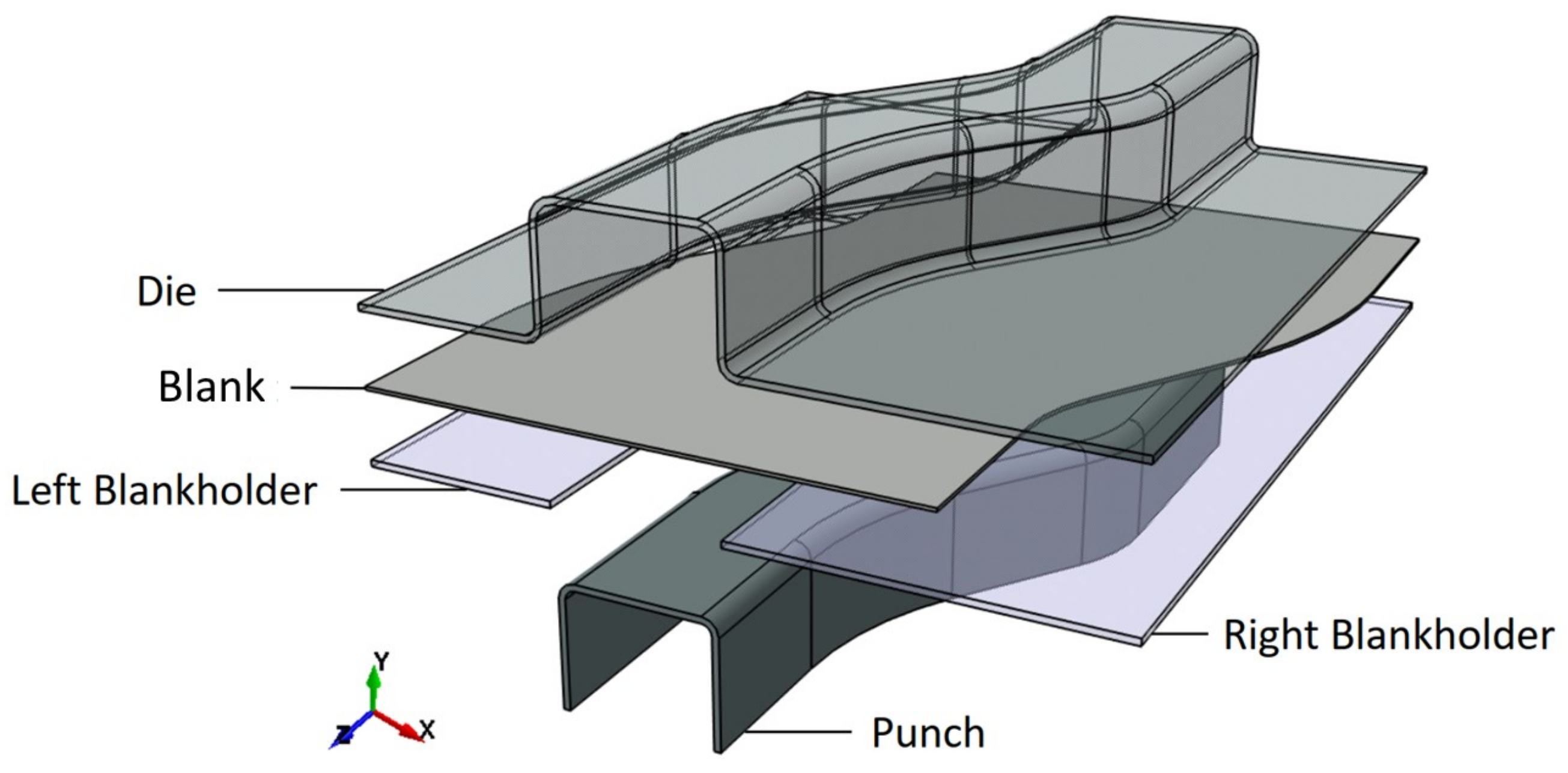
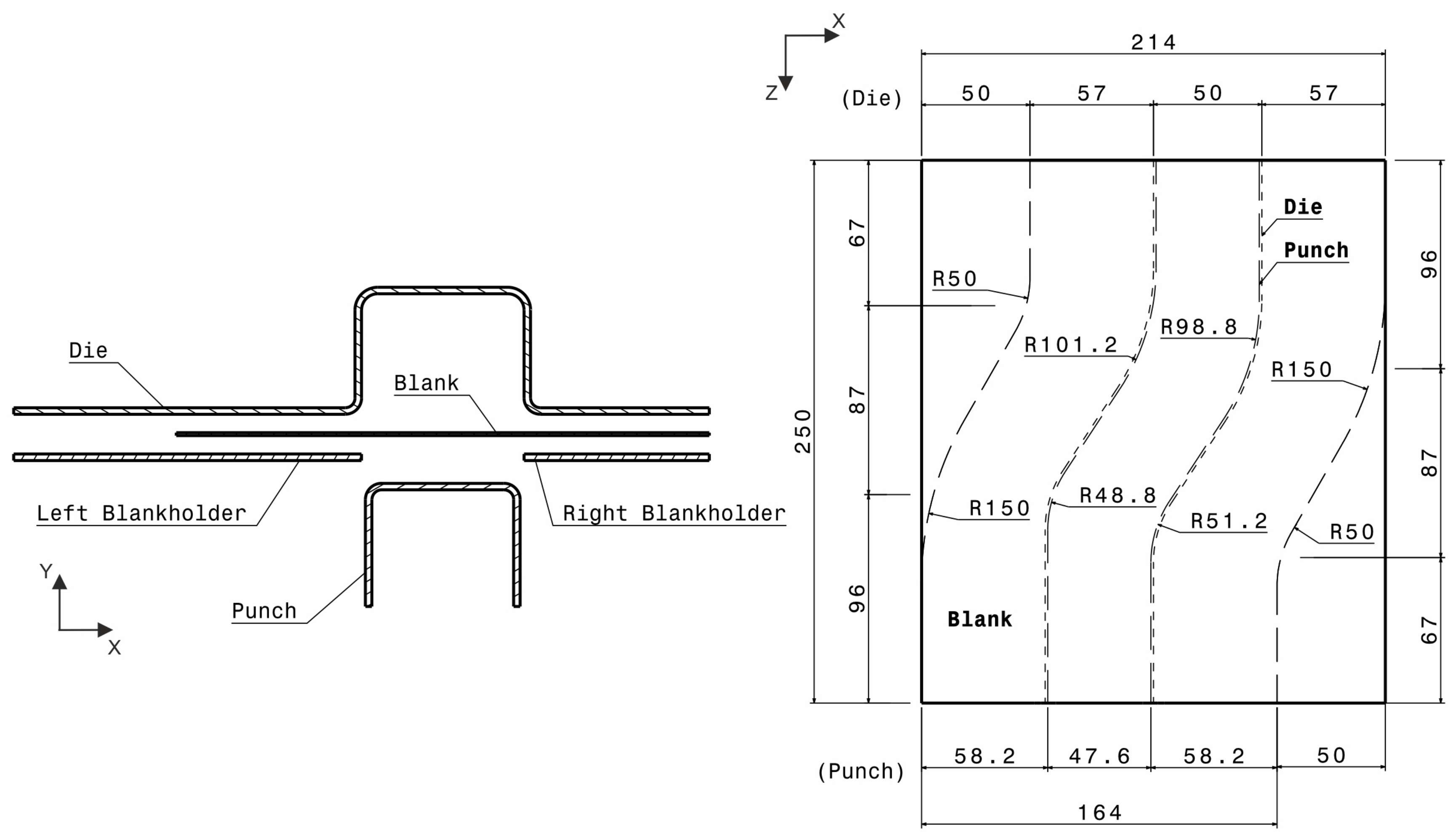
2. S-Rail Simulation

During this study, the S-Rail metal forming process is implemented in ANSYS Workbench environment, by using LS-Dyna integrated solver. The assembly configuration consists of the rigid forming tools (punch, die, blankholders), and a deformable blank, as shown in Figure 1 and Figure 2.

FEA Modelling

First of all, the following benchmark problem is modeled based on reference [13], while particularly the values of some of its parameters were utilized in the current analysis model as well. During that process, the specimen is clamped between the die and the blankholders. The punch moves upwards in order to bend the blank until reaching a full punch stroke of 37 mm. Subsequently, the tools are removed, in order to allow the specimen to be elastically unloaded since in that current study the geometry of the metal specimen is investigated before and after springback. Both states will be simulated through FEM, by using Explicit and Implicit solver, respectively.

Initially, the width and the length of the workpiece are 164 mm and 250 mm respectively, while its thickness is 0.92 mm. In addition, the punch reaches a maximum speed of 468 mm/s, which follows a trapezoidal velocity profile, and the Blankholder Force (BHF) is equal to 10 kN. As for the contacts between the rigid tools and blank, a SURFACE_TO_SURFACE contact type, with friction coefficient equal to $m{u}_c$ = 0.10, is utilized, similarly to the value used in [13]. During that type of contact, slave and master sides are defined by segments and since it is symmetric, both slave and master nodes are checked for penetration. Concerning the mesh of the model, solid elements were utilized for the rigid tools while shell elements used for the deformable blank, due to their high efficiency in such forming processes. The number of elements differs for each part of the assembly configuration. In particular, the punch, the die and the blankholders consist of 1716, 7696 and 516 elements respectively, while the deformable blank consists of 6386 elements. Regarding the material specification, AL6111-T4 was used for the metal specimen while its properties for the numerical simulation are specified in Table 1. Density $\rho$, Young modulus E, Poisson ratio $\nu$ are provided for the elastic region. The plastic region will be modeled by using the following isotropic hardening function,

$${\sigma }_y\left(\kappa \right)={\sigma }_{y0}+Q(1-exp(-\beta \kappa ))$$

where ${\sigma }_{y0}$ is the initial yield stress, Q is the max change in size of elastic range, $\beta$ is the rate of change of elastic range size and $\kappa$ is the accumulated plastic strain. In every case the results presented here have been produced by finite element models with less than 50,000 degrees of freedom. Finer meshes have not provided substantially different results.

3. Analysis Results

In this section, FE analysis by using AL6111-T4 and BHF equal to 10 KN will be implemented. The elicited results from deformation and springback simulations are compared with the corresponding outcomes from reference [13], during which the performance of a proposed solid-shell element is investigated in the framework of deep drawing simulations and springback predictions. The main differences between the current work and S-Rail forming simulation in reference [13] are the following: the explicit and implicit instead of implicit only simulation method, the use of shell instead of solid-shell element, and the punch tool velocity which equal to 468 mm/s instead of 5 mm/s. It should be noted here that the mplicit solver is in general moreaccurate than the explicit one. Furthermore, in the analysis of springback effects, it provides more stable results without oscillations between the loading increments, which in some caseds ifluence the final shape of the metal sheet.

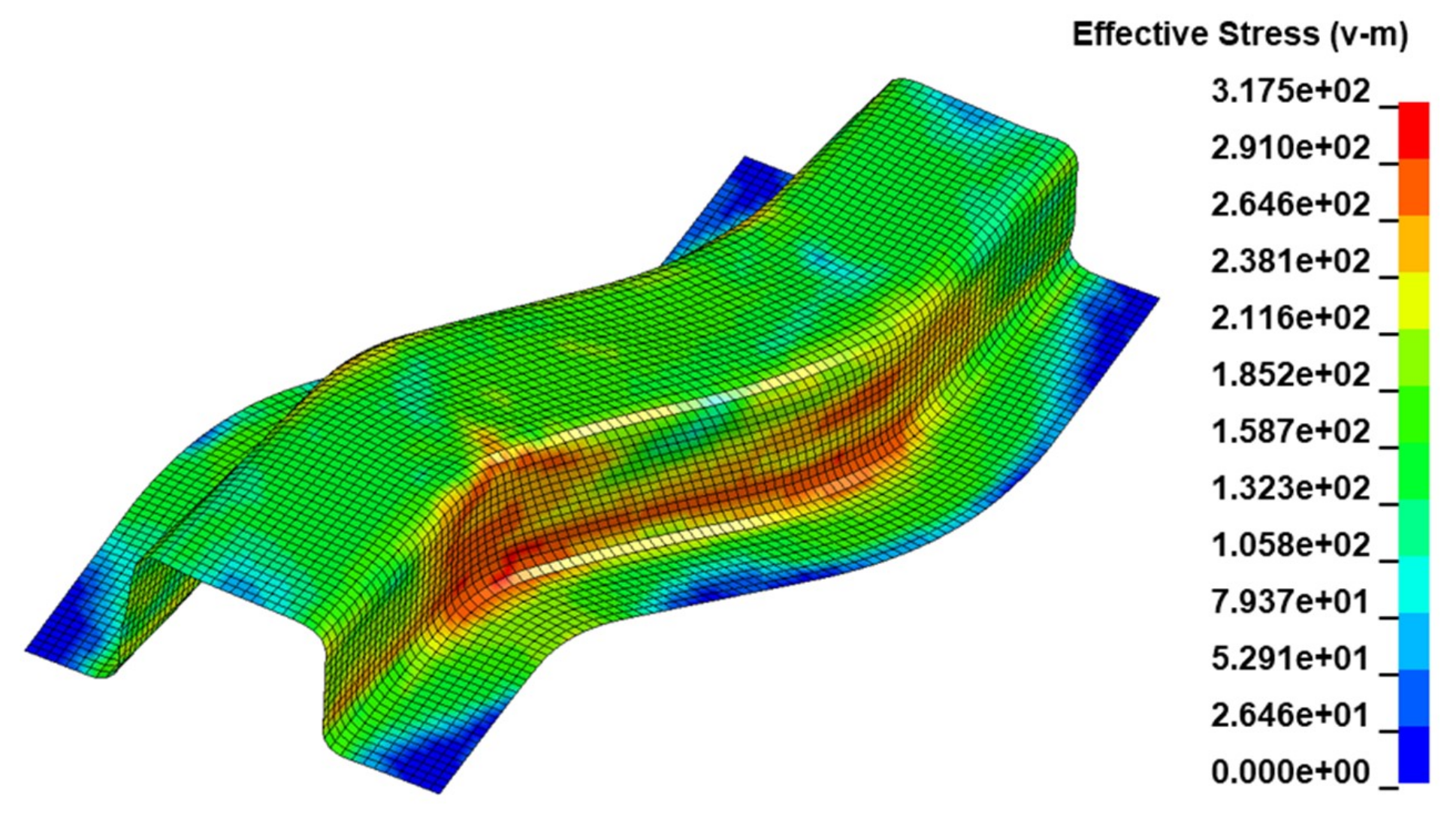
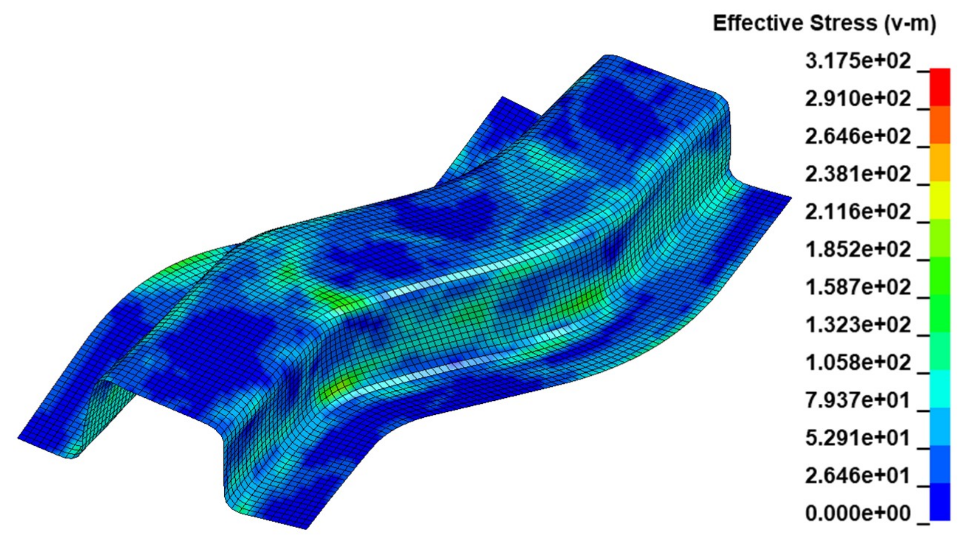
3.1. Forming Process Evaluation

After confirming that no inertial effects exist inside the simulation model, which actually means both quasi-static and energy conservation requirements are fulfilled, one should proceed to metal forming process evaluation.

3.1.1. Effective (Von-Mises) Stress

To begin with, the first step in evaluating the results contains the effective stresses of the model before springback. By looking into Figure 3, the maximum effective stress is 317.5 MPa. This is lower than the material Ultimate Tensile Strength (UTS), which is 368 MPa, which means that there are not any possibilities of necking or even crack failures. As such, the percentage error between the current work and compared simulation reaches a value of 15.4%.

Subsequently, the effective stress distribution after elastic unloading will be studied. As can be seen from Figure 4, the max effective von-Mises stress of the current model reaches a value of 238.8 MPa. Hence, the approximate percentage error between the two FE simulations reaches 15.4% as well.

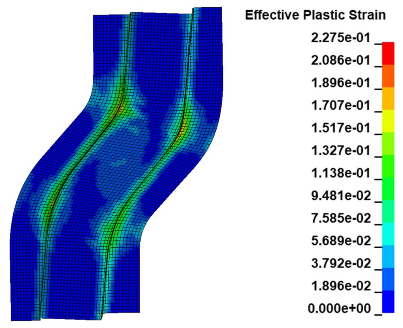
3.1.2. Effective Plastic Strain

After evaluating and comparing the effective stresses of the model, one should proceed in the plastic strain investigation. As observed in Figure 5, a maximum plastic strain of 0.2275 is reached. Thus, the approximate percentage error between the compared simulations is equal to 9.9%.

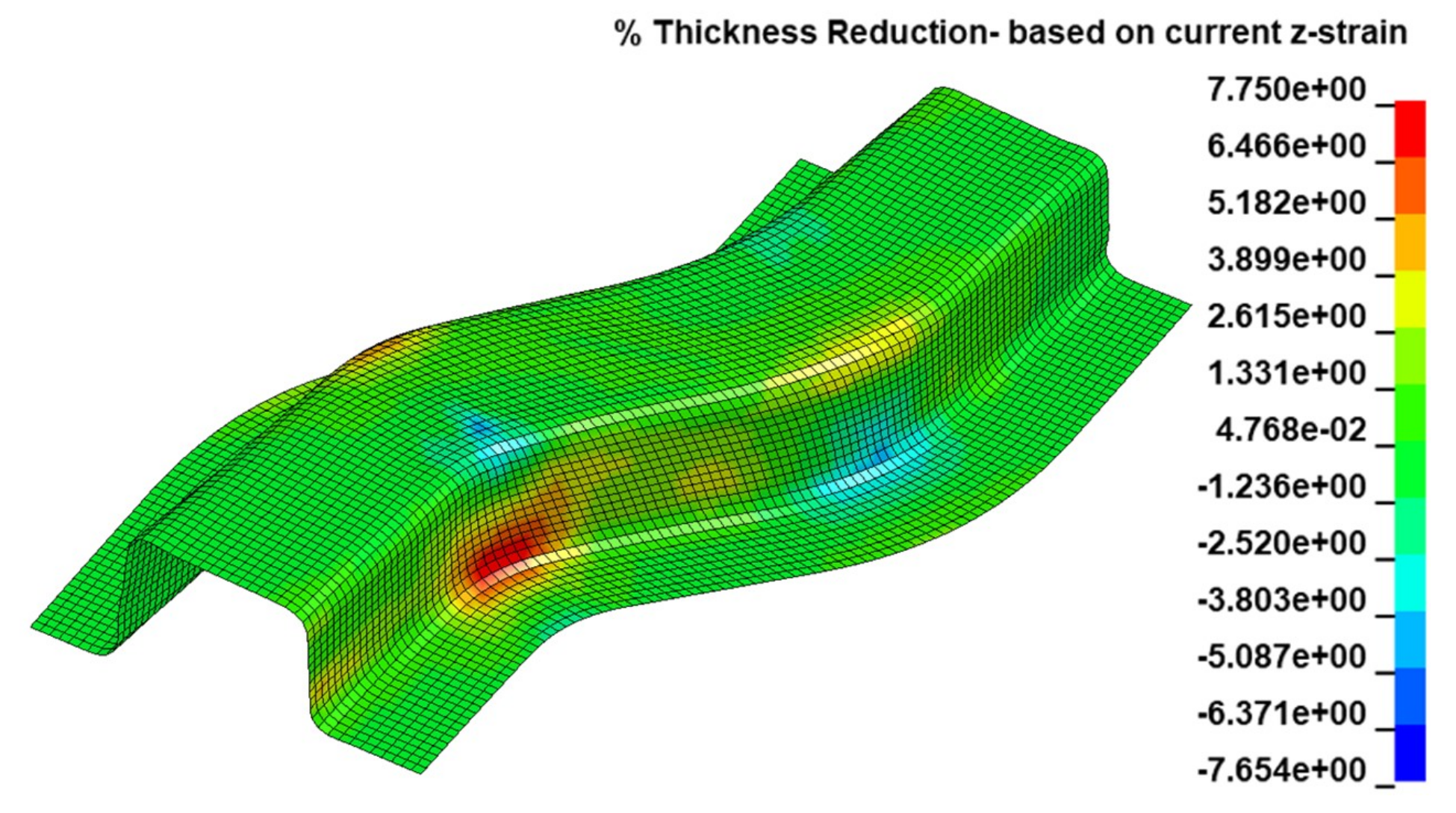
3.1.3. Material Failures Evaluation

To evaluate the material failures of the blank, one should refer to the thickness reduction plot as well as to the Forming Limit Diagram (FLD)/Strain distribution diagram. Through both of them, a good estimation can be made regarding the load that the specimen can withstand until some cracks appear.

In fact, by taking a look at the thickness reduction plot below in Figure 6, one can observe that the thickness is within a range of −7.65% to 7.75%, with an initial thickness of 0.92 mm. The material thinning is not that high to provoke cracks on the metal workpiece. In order to confirm that this prediction is correct, the FLD plot, as well as the strain distribution diagram, should be studied.

By taking a look at the FLD/Strain distribution plot, Figure 6, one can get an idea about the amount of thickness reduction the material can withstand before any cracks occur. As can be observed from the plot, there is no indication for cracks, not even for risks of cracks, which is a very good sign. Such results seem to be reasonable and by combining them with the low material thinning values, the assumption made at the beginning is confirmed. Now apart from the thinning, something also important to notice is the thickening of the specimen. There are many wrinkled areas and many areas that tend to wrinkle. If one checks again the thickness reduction plot, Figure 6, it can be confirmed that the wrinkling failures occur where thickening is indicated, as depicted in both formability and FLD plots, Figure 7 and Figure 8 respectively. However, to further investigate those results, one can detect the exact location of those wrinkles, by observing the plain geometry in Figure 9, and as such, it can be seen that some of the wrinkling areas indicated, does not even exist on the model surface. So, one can conclude in the fact that forming limit diagram should be used with caution when it comes to wrinkling evaluation because sometimes it can miss some indications.

Mesh size influences marginally the results in the sense that the general picture of wrinkling remains the same and only some small details change. The used mesh provides a reliable estimate of the results, by keeping a reasonable accuracy-to-cost ratio.

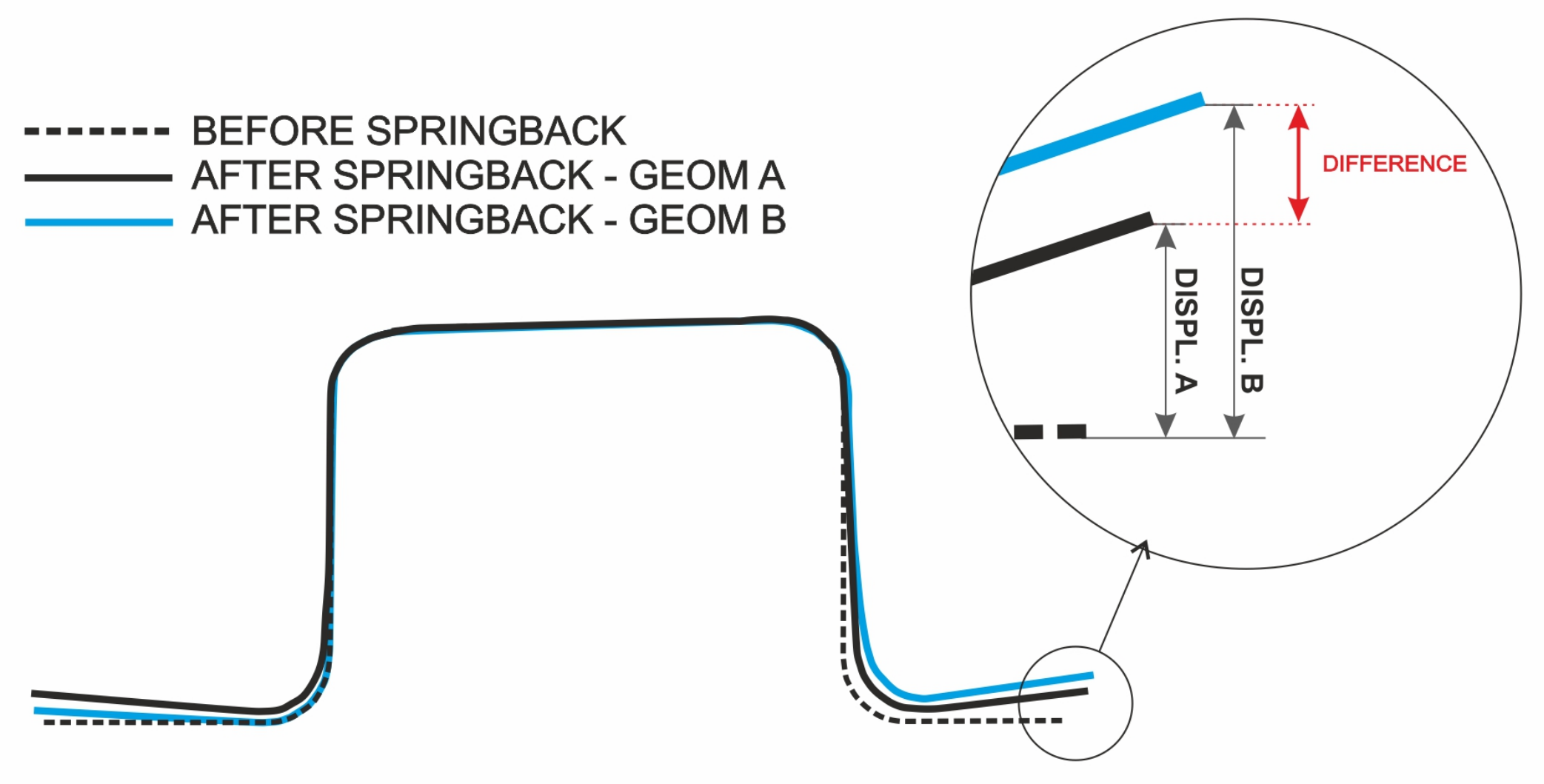
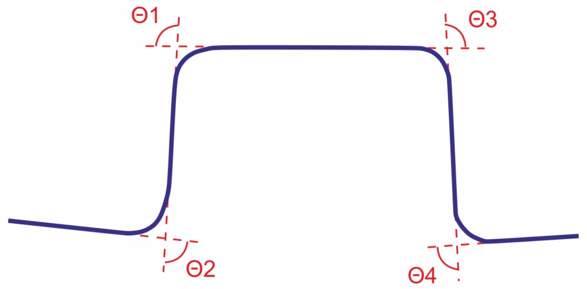
3.2. Springback Prediction

After the forming process finishes, the next step is springback evaluation. To quantify springback, two path lines J–D and I–E were considered, see in Figure 10. One section cut will be applied per corresponding path line. Afterward, along these section cuts, “before springback” and “after springback” states will be plotted. Subsequently, a comparison will be made between the blank z-axis displacements during “after springback” states, considering results from current analysis and reference [13] simulation, as shown in Figure 11. Thus, the actual displacement difference between them will be investigated.

To start with, as for the first section cut along the path J–D, by looking into Figure 12, one can observe the geometry change of the specimen after elastic unloading. Subsequently, a comparison between the states “after springback” of both current analysis results and those from reference [13] simulation, is implemented. By looking into a more detailed way, the displacement differences are 0.16 mm and 0.26 mm, for the J and D section side, respectively.

Afterward, the second section cut along the path I–E will be investigated. As depicted in Figure 13, one can again observe the displacement of the specimen in the current analysis between the “before” and “after” springback states. Subsequently, a comparison between the “after elastic unloading” states of the current analysis and the corresponding simulation from [13], is implemented. As can be seen, the displacement discrepancies are 1.17 mm and 2.02 mm for the I and E section sides, respectively. Thus, one can observe that the displacements along the I–E path, are larger than those along J–D.

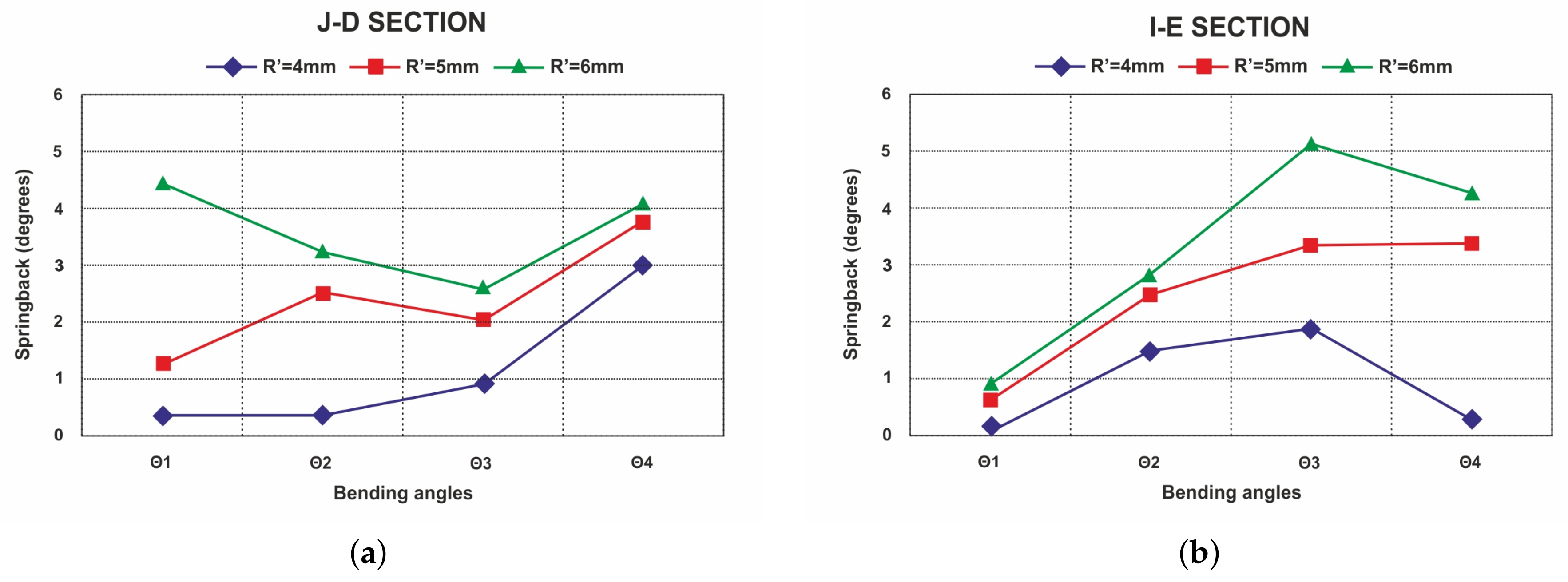
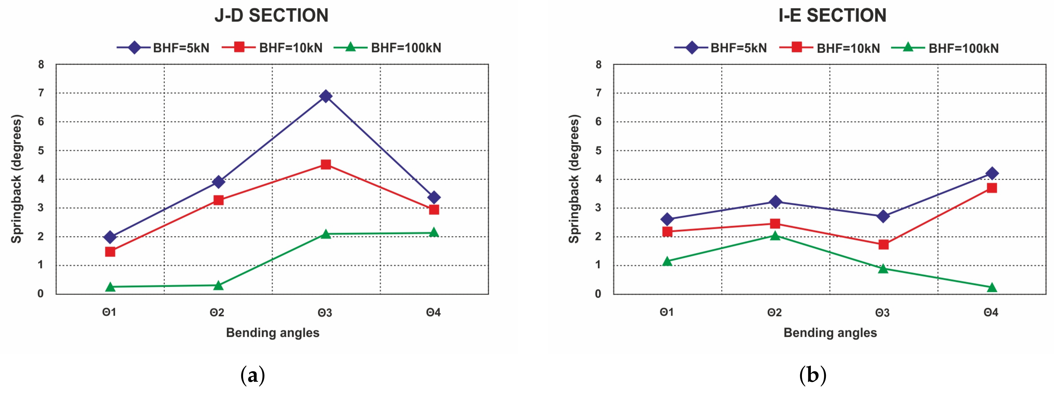
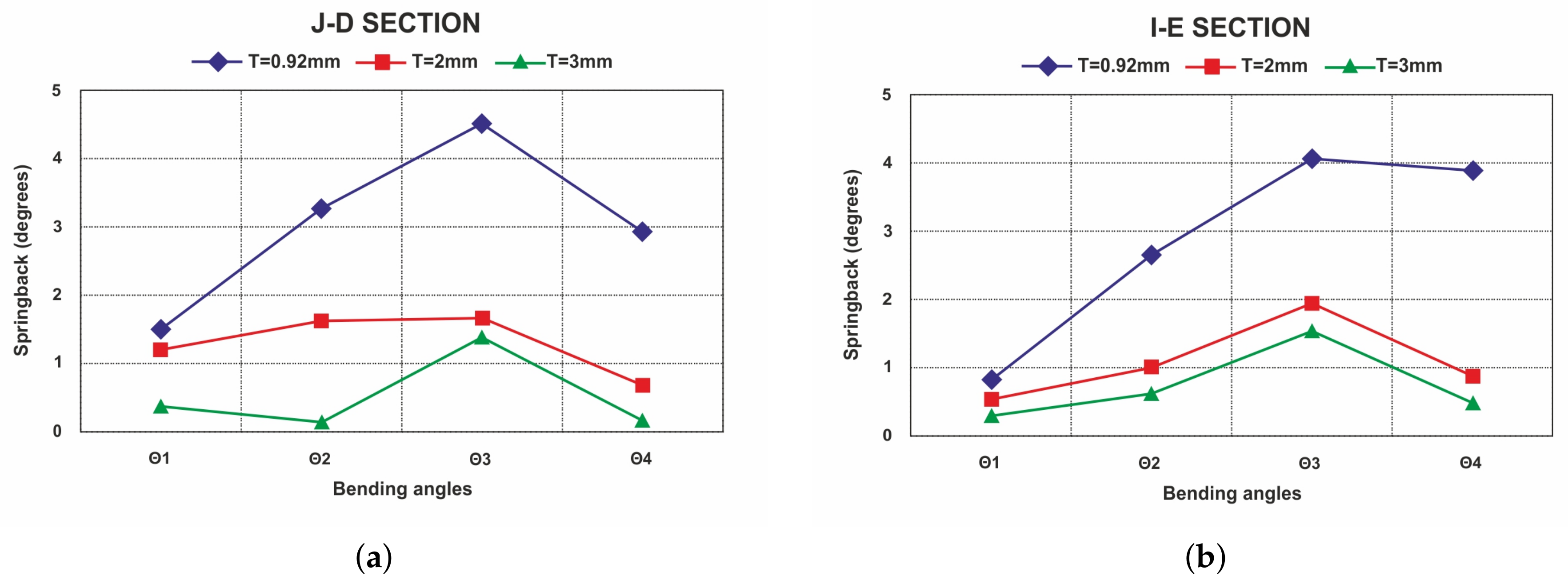
4. Springback Sensitivity Evaluation

In order to observe springback sensitivity, some parameters of the current model will be modified and then the elicited results will be evaluated. The springback will be investigated again along J–D and I–E, see Figure 10, but currently it will be quantified through the $\mathsf{\Theta }1,\mathsf{\Theta }2,\mathsf{\Theta }3,\mathsf{\Theta }4$ angles of the specimen, as depicted in Figure 14.

4.1. Effects of Tools Radius

First of all, in order to investigate the elastic unloading sensitivity during the punch and die radii change, a number of FE simulations will be executed, and in each one of them, the geometry tools will have a different radius, 4 mm, 5 mm, and 6 mm. During those simulations, the material AL6111-T4 will be utilized, the blankholder force will remain equal to 10 KN and the sheet thickness will not change. Therefore, by taking a look at the results, it can be observed that in both sections cuts J–D and I–E, as shown in Figure 15 respectively, by increasing the values of tool radiuses the springback of the workpiece increases as well. Hence, what already stated in [4,14,15] is confirmed.

4.2. Effects of BHF

In order to observe the effect of blankholder force (BHF) on elastic material unloading, FE simulations with BHF values of 5 KN, 10 KN and 100 KN will be executed, on an AL6111-T4 metal workpiece with thickness 0.92 mm. The obtained results are listed in Figure 16, so by looking in more detail, one can detect that elastic unloading decreases as the BHF increases in both section paths. Thus, what is already mentioned in [16,17,18] is confirmed. Additionally, that phenomenon is reasonable because when applying low BHF, punch induces mostly bending stresses in the material. On the contrary, when blankholder force increases, the stresses induced by the punch become mostly tensile stresses [15].

4.3. Effects of Sheet Thickness

Apart from springback sensitivity in radius and BHF, elastic unloading is also sensitive in sheet thickness alteration. Hence, in order to study that phenomenon, a number of simulations will be executed, by using sheet metal specimens with a gradually increased thickness of 0.92 mm, 2 mm, and 3 mm. The BHF will remain equal to 10 KN, and AL6111-T4 material will be utilized. By looking into Figure 17, one can clearly observe that while the sheet metal thickness increases, springback gradually decreases. Such behavior confirms what is already mentioned in [4,14].

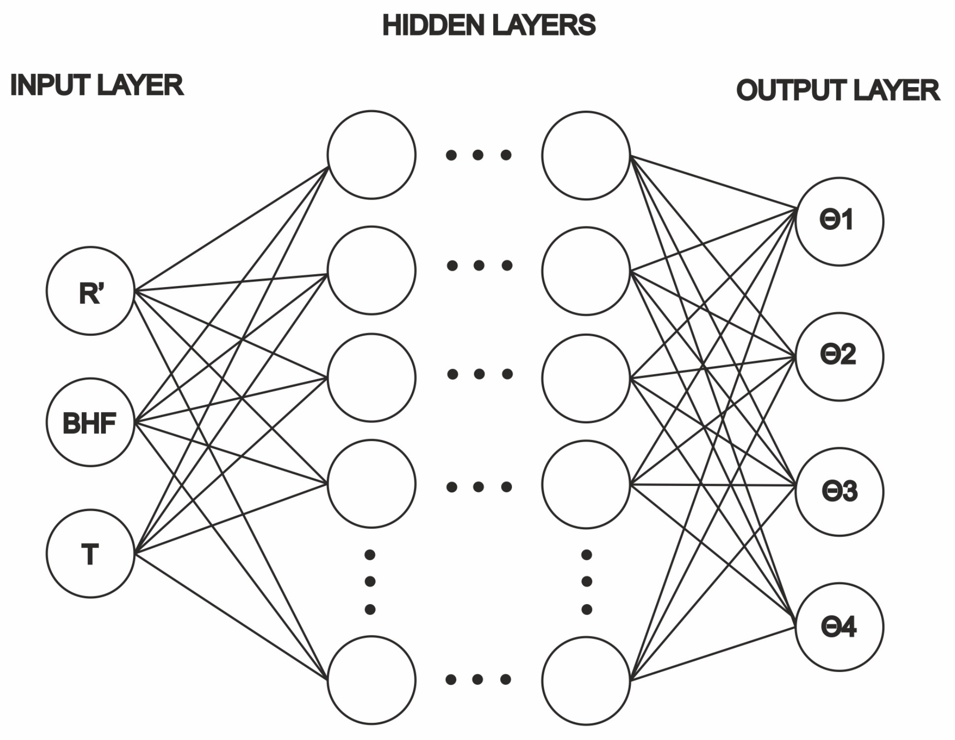
5. The Artificial Neural Network Metamodel

5.1. Artificial Neural Networks

A neural network is a set of fundamental processing elements or neurons and connections with adjustable weights, attempting to simulate the human brain as well as the biological neural networks function. ANNs have been successfully used to solve problems in various sectors such as engineering, neurology, medicine, mathematics, and others [19]. In case of a multi-layer NN, the network consists of an input layer, one or more hidden layers and an output layer. The first one is the layer that receives the already provided experimental results, which will be used as training data for the ANN. Concerning the hidden layer, it receives the data from input layer and after processing it, the results are conveyed to the output layer. Last but not least, the output layer receives all the responses from hidden layer, and exports a corresponding output. The ANN structure is depicted in Figure 18.

Each layer has a number of processing elements connected by links with adjustable synaptic weights. The output of each neuron is provided by

$$S_i=\sum _{j=1}^n{x}_j{w}_{ij}+b_j$$

where n is the number of inputs, $x_j$ is the value received from the previous neuron, $w_{ij}$ is the weight between i and j neurons and $b_j$ is the bias of the neuron. The output of the neuron is given by the following equation

$$y_j=f\left(S_i\right)$$

where f is the transfer or activation function.

An ANN that can be trained with the backpropagation algorithm, stores the experimentally gained knowledge by optimizing its parameters, i.e., synaptic weights based on the actual relationship between the provided input and output sets [3]. The error is described by the Mean-Squared Error (MSE) and is given as follows

$$MSE=\frac{1}{n}\sum _{j=1}^n{(t_j-a_j)}^2$$

where n is the number of sets that include input and output data, $a_j$ are the output based on the input values while $t_j$ are the corresponding predicted output values. Training with Bayessian method is suitable in case of small data sets, as it is in the preliminary investigation reported in this paper [20].

In order to define the optimal ANN structure to be used for the current model prediction, a script was performed in MATLAB environment, through which a large number of different ANN structure scenarios were implemented. The optimal architecture was selected based on each predictor’s performance, which was accessed through mean-squared error (MSE) and regression coefficient (R) between the output ANN results and the provided target values.

In particular, the input experimental values used in the current study consist of 13 datasets, as depicted in

Table 2. Finite element analysis (FEA) springback datasets for artificial neural network (ANN).

No.	Tool Radius	Blankholder Force	Sheet Thickness	$\mathit{\theta }1$ Angle	$\mathit{\theta }2$ Angle	$\mathit{\theta }3$ Angle	$\mathit{\theta }4$ Angle
1	4	10	0.92	0.36	0.36	0.91	3.01
2	5	20	0.92	1.48	2.61	2.18	3.85
3	6	10	0.92	4.45	3.24	2.57	4.08
4	5	5	0.92	1.98	3.97	6.86	3.15
5	5	50	0.92	1.58	3.38	4.46	2.87
6	5	100	0.92	0.28	0.30	2.10	2.16
7	5	10	0.92	1.49	3.27	4.52	2.93
8	5	10	2	1.19	1.62	1.57	0.67
9	5	10	3	0.37	0.12	1.43	0.12
10	4	5	0.92	1.06	2.06	0.24	2.88
11	4	100	0.92	2.92	1.18	1.76	2.07
12	6	15	0.92	2.79	2.79	3.99	1.98
13	6	100	0.92	1.93	1.23	0.09	4.80

, which were split into two different groups, one for training, and one for testing with ratios 0.8 and 0.2, respectively. The networks were trained through Bayesian regularization backpropagation (trainbr). As such, the optimum ANN selected architecture is 3-16-4. The architecture is based on the feed-forward Multilayer Perceptron (MLP) Neural Network which consists of 1 input layer with 3 inputs (Tool radius, BHF, Sheet thickness), 1 hidden layer having 16 hidden neurons, and 1 output layer with 4 outputs (angles of the specimen).

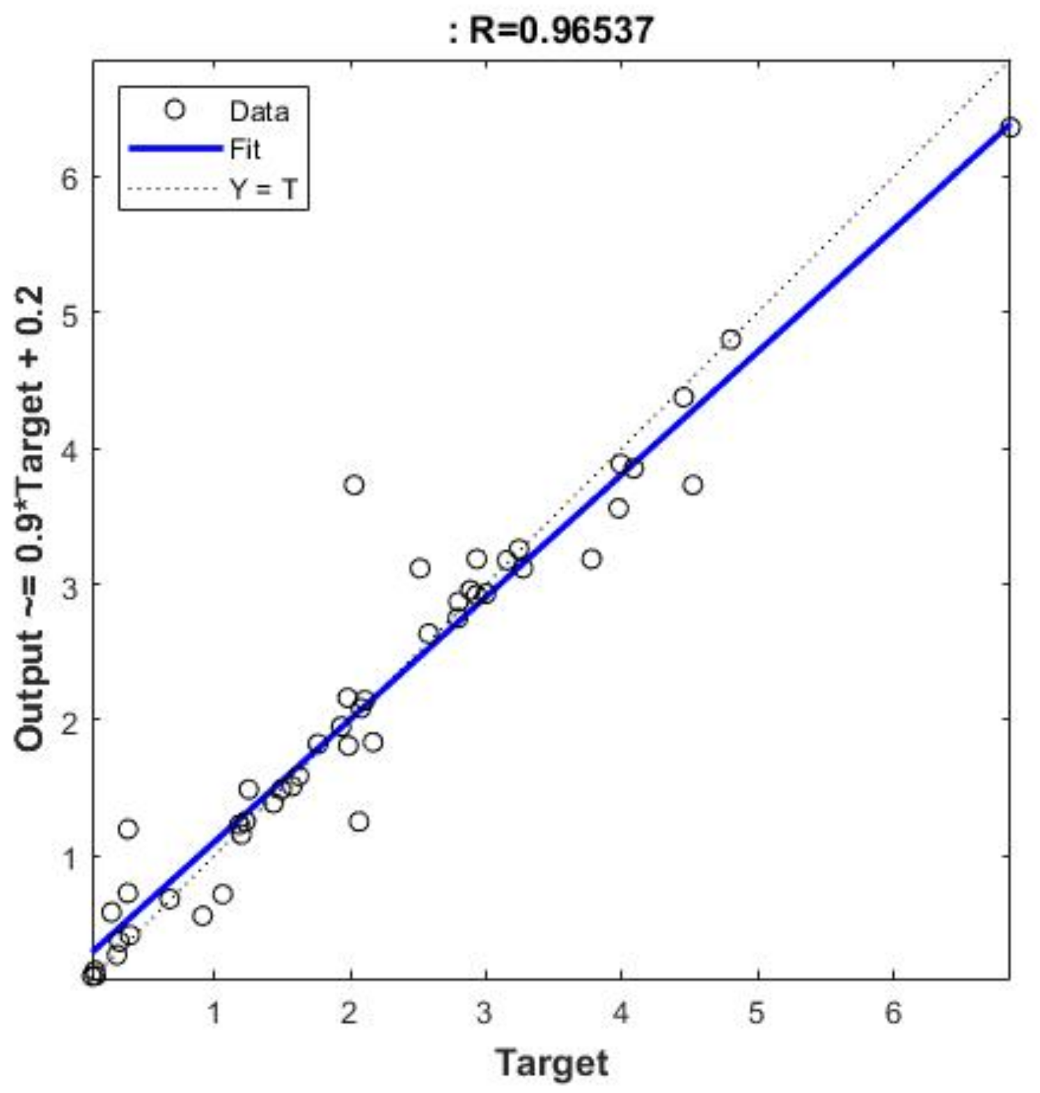
5.2. Springback Prediction with ANN

As mentioned above, the results obtained from FEA simulations were used to train the neural networks. Several networks were investigated considering various scenarios with different numbers of hidden layers, as well as different quantity of neurons inside each hidden layer. All the possible ANN cases were accessed through a MATLAB script, and eventually the one with the lowest generalization error was selected as the representative. The mean-squared error (MSE) value of the optimum network was the minimum one, and it was equal to 0.1473. Thus, after its optimal architecture was defined and trained properly, springback angle predictions were implemented based on different tools radius (R’), blankholder force (BHF) and sheet thickness (T) combinations. Subsequently, a comparison between FEA and ANN prediction results was conducted for all four angles of the deformable specimen ($\mathsf{\Theta }1,\mathsf{\Theta }2,\mathsf{\Theta }3,\mathsf{\Theta }4$), from Figure 14, and eventually a good agreement was achieved, as can be observed in Figure 19.

Additionally, in order to investigate the ANN performance in a more detailed way, one can implement a regression analysis as well as calculate the dispersion around the “Y = T” line. Therefore the regression coefficient is equal to 0.9653, as depicted in Figure 20, while the mean average deviation is receives a value equal to 1.1673. As such the performance of the ANN, seems to be adequate for the current study.

6. Conclusions

In this study, an innovative neural network system which predicts springback in sheet metal forming processes is proposed. For the ANN training purposes a number of examples were created, through a carefully prepared simulation of an S-Rail configuration. After validating the FE model for a test case used in similar industrial studies, a number of springback predictions were implemented by means of the Bayesian regularized backpropagation neural network.

With regards to the conclusions drawn from this study, during the FE model simulation one can observe that errors reach values of 15.4% and 9.9% in stresses and plastic strains plot, respectively. Subsequenlty, no strange indications concerning material failures detected, except for some wrinkling phenomena, at specific areas. During springback state, the maximum discrepancies between the two unloaded geometries reach values of 0.26 mm and 2.02 mm, for the D side and E side respectively. Considering the fact that the current analysis is a complex shaped problem, the material used was nonlinear, as well as some model parameters like mesh elements, punch velocity, etc., were differentiated from compared simulation, one can say that those error levels could be reasonable.

Last but not least, with regards to the neural network approach, springback predictions were implemented in the current sheet metal forming application. The neural networks were trained through Bayesian backpropagation algorithm (trainbr) by using 13 data sets as input, while after several trials with different network architecture scenarios, the optimum one selected was 3-16-4. A mean squared error, a regression coefficient and a mean average deviation equal to 0.1473, 0.9653 and 1.1673, respectively, were achieved. Consequently, as can be noticed, a good agreement between the target and predicted output values has been accomplished.

References

1. Teti, R.; Engel, U. Numerical Simulation of Metal Sheet Plastic Deformation Processes through Finite Element Method. Ph.D. Thesis, University of Naples Federico II, Naples, Italy, 2006. [Google Scholar]
2. Jadhav, S.; Schoiswohl, M.; Buchmayr, B. Applications of Finite Element Simulation in the Development of Advanced Sheet Metal Forming Processes. BHM Berg-und Hüttenmännische Monatshefte 2018, 163, 109–118. [Google Scholar] [CrossRef] [Green Version]
3. Kazan, R.; Fırat, M.; Tiryaki, A.E. Prediction of springback in wipe-bending process of sheet metal using neural network. Mater. Des. 2009, 30, 418–423. [Google Scholar] [CrossRef]
4. Gawade, S.; Nandedkar, V. Investigation of springback in U shape bending with holes in component. Ind. Eng. J. 2018, 11. [Google Scholar] [CrossRef]
5. Mulidrán, P.; Šiser, M.; Slota, J.; Spišák, E.; Sleziak, T. Numerical Prediction of Forming Car Body Parts with Emphasis on Springback. Metals 2018, 8, 435. [Google Scholar] [CrossRef] [Green Version]
6. Panthi, S.K.; Hora, M.S.; Ahmed, M.; Materials, C.A. Artificial neural network and experimental study of effect of velocity on springback in straight flanging process. Indian J. Eng. Mater. Sci. 2016, 23, 159–164. [Google Scholar]
7. Ruan, F.; Feng, Y.; Liu, W. Springback Prediction for Complex Sheet Metal Forming Parts Based on Genetic Neural Network. In Proceedings of the 2008 Second International Symposium on Intelligent Information Technology Application, Shanghai, China, 20–22 December 2008; pp. 157–161. [Google Scholar]
8. Han, F.; Mo, J.H.; Qi, H.W.; Long, R.F.; Cui, X.H.; Li, Z.W. Springback prediction for incremental sheet forming based on FEM-PSONN technology. Trans. Nonferrous Met. Soc. China 2013, 23, 1061–1071. [Google Scholar] [CrossRef]
9. Marretta, L.; Di Lorenzo, R. Influence of material properties variability on springback and thinning in sheet stamping processes: A stochastic analysis. Int. J. Adv. Manuf. Technol. 2010, 51, 117–134. [Google Scholar] [CrossRef]
10. Prates, P.A.; Adaixo, A.S.; Oliveira, M.C.; Fernandes, J.V. Numerical study on the effect of mechanical properties variability in sheet metal forming processes. Int. J. Adv. Manuf. Technol. 2018, 96, 561–580. [Google Scholar] [CrossRef]
11. Dib, M.; Ribeiro, B.; Prates, P. Model Prediction of Defects in Sheet Metal Forming Processes. In Engineering Applications of Neural Networks; Pimenidis, E., Jayne, C., Eds.; Springer: Cham, Switzerland, 2018; Volume 893, pp. 169–180. [Google Scholar]
12. Dib, M.A.; Oliveira, N.J.; Marques, A.E.; Oliveira, M.C.; Fernandes, J.V.; Ribeiro, B.M.; Prates, P.A. Single and ensemble classifiers for defect prediction in sheet metal forming under variability. Neural Comput. Appl. 2019. [Google Scholar] [CrossRef] [Green Version]
13. Schwarze, M.; Vladimirov, I.N.; Reese, S. Sheet metal forming and springback simulation by means of a new reduced integration solid-shell finite element technology. Comput. Methods Appl. Mech. Eng. 2011, 200, 454–476. [Google Scholar] [CrossRef]
14. Alghtani, A.H. Analysis and Optimization of Springback in Sheet Metal Forming. Ph.D. Thesis, The University of Leeds, West Yorkshire, UK, 2015. [Google Scholar]
15. Papeleux, L.; Ponthot, J.P. Finite element simulation of springback in sheet metal forming. J. Mater. Process. Technol. 2002, 125, 785–791. [Google Scholar] [CrossRef]
16. Choi, J.; Lee, J.; Bae, G.; Barlat, F.; Lee, M.G. Evaluation of Springback for DP980 S Rail Using Anisotropic Hardening Models. JOM 2016, 68, 1850–1857. [Google Scholar] [CrossRef]
17. Chirita, B.; Brabie, G. Control of Springback Intensity in U-Bending through variation of Blankholder force. In Proceedings of the 9th International Research/Expert Conference Trends in the Development of Machinery and Associated Technology, Antalya, Turkey, 26–30 September 2005; pp. 175–178. [Google Scholar]
18. Jiang, K.; Hou, Y.; Lin, J.; Min, J. A springback energy based method of springback prediction for complex automotive parts. IOP Conf. Ser. Mater. Sci. Eng. 2018, 418, 012104. [Google Scholar] [CrossRef]
19. Bozdemir, M.; Golcu, M. Artificial Neural Network Analysis of Springback in V Bending. J. Appl. Sci. 2008, 8, 3038–3043. [Google Scholar] [CrossRef]
20. Okut, H. Bayesian Regularized Neural Networks for Small n Big p Data. In Artificial Neural Networks. Methods and Applications; Rosa, J.L.G., Ed.; Intech Open Book: London, UK, 2016; pp. 16–48. ISBN 978-953-51-2705-5. [Google Scholar] [CrossRef]
Figure 1. Geometrical assembly configuration of the S-Rail forming process.
Applmech 01 00007 g001
Figure 2. S-Rail configuration drawings.
Applmech 01 00007 g002
Figure 3. Effective von-Mises stresses plot before springback.
Applmech 01 00007 g003
Figure 4. Effective von-Mises stresses plot after springback.
Applmech 01 00007 g004
Figure 5. Effective plastic strain plot.
Applmech 01 00007 g005
Figure 6. Thickness reduction plot.
Applmech 01 00007 g006
Figure 7. Formability plot.
Applmech 01 00007 g007
Figure 8. Forming Limit Diagram (FLD) plot.
Applmech 01 00007 g008
Figure 9. Plain geometry with wrinkling indications.
Applmech 01 00007 g009
Figure 10. J–D and I–E section cut paths.
Applmech 01 00007 g010
Figure 11. Blank displacement measurement, between “before” and “after” springback states. Implemented on both sides of each specimen section cut.
Applmech 01 00007 g011
Figure 12. (a) Workpiece deformation before and after springback in section J–D (b) After springback z-axis displacement comparison between reference [13] and current analysis.
Applmech 01 00007 g012
Figure 13. (a) Workpiece deformation before and after springback in section I–E (b) After springback z-axis displacement comparison between reference [13] and current analysis.
Applmech 01 00007 g013
Figure 14. Springback measurement angles.
Applmech 01 00007 g014
Figure 15. Springback comparison between different tools radiuses through (a) J–D (b) I–E section paths.
Applmech 01 00007 g015
Figure 16. Springback comparison between different blankholder forces through (a) J–D (b) I–E section paths.
Applmech 01 00007 g016
Figure 17. Springback comparison between different sheet thicknesses through (a) J–D (b) I–E section paths.
Applmech 01 00007 g017
Figure 18. Neural Network structure.
Applmech 01 00007 g018
Figure 19. Comparison between FEA and ANN prediction results of springback angles.
Applmech 01 00007 g019
Figure 20. Neural network predicted output results vs. FEA simulation target values regression.
Applmech 01 00007 g020