Conformal Wireframe Nets for Trimmed Symmetric Unit Cells in Functionally Graded Lattice Materials


Department of Mechanical and Aerospace Engineering, Carleton University, Ottawa, ON K1S 5B6, Canada
*
Author to whom correspondence should be addressed.
Appl. Mech. 2021, 2(1), 81-107; https://0-doi-org.brum.beds.ac.uk/10.3390/applmech2010006
Submission received: 29 January 2021
/
Revised: 20 February 2021
/
Accepted: 23 February 2021
/
Published: 28 February 2021
Abstract
:Tessellating a periodic unit cell of lattice material to fill a design space in complex geometries has many challenges arising from their computer-aided design (CAD) modeling intricacy. A solution to this difficulty is the use of trimmed micro-truss lattice structures with a conformal net. This paper presents a novel algorithm for constructing conformal lattice net as wireframe of one-dimensional line segments suitable for Bravais cubic symmetric truss-based topologies. The novel algorithm is an excellent candidate when dealing with lattice structures using cubic, body-centered cubic (BCC), face-centered cubic (FCC), and/or diamond unit cell configurations. The wireframe structure is easily transferred into one-dimensional beam elements for microscale optimizations to obtain a functionally graded lattice material. It is shown that introduction of the lattice net resulted in a significant reduction in the mass of the optimized design.
1. Introduction
A periodic micro-truss structure, also known as truss lattice or lattice material, is generated by tessellating a unit cell in a 2D or a 3D infinite periodicity. The most common example of a truss lattice material is the cubic and BCC unit cell. Truss lattice materials expand materials selection design space through providing meta-materials for advanced engineering applications [1]. The high specific properties of lattice materials make them an attractive hybrid material to save weight and costs [2]. However, due to their complex geometries, manufacturing such microstructures was near impossible a few decades ago. Nevertheless, lattice materials have been gaining popularity due to the advancements in additive manufacturing.
Due to the complexity of the micro-structure of truss lattice materials, where it involves a huge number of elements, the possibility of solving all underlying equations in full detail is computationally expensive and might be impossible. Accordingly, the laws of greatest importance are the principles of symmetry where the lattice is modeled through a unit cell. Such concept in continuum mechanics finds its roots in solid-state physics where a lattice is mainly concerned with replicating the strengths from atomic bonds commonly seen in metals and metallic alloys. Examples of atomic bonds and their strengths can be seen in diamonds where carbon atoms share all their valence electrons with other neighboring carbon atoms forming what is called a diamond lattice. The structure of the diamond lattice is known to have the highest tensile strength among all atomic topologies and could be a good candidate for creating strong micro lattice structures [3,4]. The number of possibilities for lattice topologies is endless. However, only symmetrical lattice structures with clear crystallographic planes are considered in this paper. The most common symmetric lattice topologies which are also analyzed in this paper include unit cells with Cubic and Body-Centered Cubic (BCC), Face-Centered Cubic (FCC), and diamond geometries [5].
There exist many methods for modeling truss lattice structures in computer-aided design (CAD). These range from the utilization of voxels to implicit surface definitions to generate the interior and exterior lattice topologies [6,7,8,9]. When it comes to implementing lattice structures into a design, there exists three main strategies [6]. The first is a swept interior lattice which distorts the lattice to meet the curvature of the design domain. The second is by directly meshing the design domain with elements and then converting those elements into the desired unit cell topology afterwards. The third is a trimmed interior where the periodic lattice pattern is conserved and is then truncated once outside the design domain. Sweeping methods require significant user intervention as well as panning and are very time consuming to produce. The problem is more apparent for complex geometries where transitions between sections does not guarantee a consistent unit cell size. Meshed domains also require a user defined mesh, which can be time consuming. However, if the unit cell size is changed, then the entire mesh will be required to be redone. The unit cell size could also be inconsistent and is subject to warping in the vicinity of curved geometries.
There are many advantages for swept and meshed lattice regions such as ease of application and limited complexity in modeling. The exterior of a domain can also be easily closed off using the correct lattice topology. However, connecting the exterior struts of the trimmed lattice is not as easily defined, especially in three-dimensional lattice configurations. An exterior mesh of structures connecting interior struts together is known as a conforming skin, lattice net, or a conformal lattice net [6].
Many of the proposed methods focus on modeling the interior lattice and omit the lattice connections on the surface. Some CAD applications, such as NX [10,11,12], opt for Delaunay triangulation to connect the lattice at the surface, which is considered among the simplest solutions. The drawback of using Delaunay triangulation for a lattice net is its dissociation from the interior lattice geometry does not always match the interior lattice geometry. The most robust lattice creation tool in the market currently is nTopology [13], which offers a suite of tools to insert a wide array of lattices. Sweeping, Voronoi meshing, and implicit modeling are available to users, however connecting trimmed lattices together at the surface is not supported [13]. Intralattice [14] is another lattice creation tool which presents the user with many options for inserting lattice into a closed volume which also includes trimmed lattice creation using rhino [15]. Unfortunately, at this time of writing, there is no option to connect the cut struts together to create a conformal lattice net using Intralattice. One open-source MATLAB code known as GIBBON, developed by Moerman, allows its users to create and optimize meshes of lattices structures inside complex geometries. However, trimmed lattices are not available [16].
Current research in conformal lattices focus on the meshing approach instead of trimmed lattices. Sosin et al. [17] utilized sphere packing to automatically generate conformal strut connections in any volume and offer two compatible truss topologies. The trade off to Sosin et al.’s methods is that it is not applicable for trimmed lattices. Another research into conforming lattices is by Wu et al. [18], who combined homogenization and topology optimization to develop lattice structures which conform to principal stress directions and the enclosed boundaries. The resulting structure contains a lattice net which conforms to the interior lattice; however, it is not a trimmed lattice. Finally, Liang et al. developed an algorithm to create conformal lattice structures on parametric solid models and which also includes a lattice net generation procedure [19]. The work of Liang et al. also includes solid shell (or skin) creation in place of the lattice net and will generate a NURBS representation of the new object. Liang et al.’s methods will fit the interior lattice to follow the boundary of the closed geometry which will not produce an interior trimmed lattice structure.
There are several advantages for selecting a trimmed lattice over the other two methods including the lack of user intervention when generating the mesh as it can be automated, unit cells are not distorted due to curved geometries and can be oriented in any direction, in addition, the unit cell size is also independent of the geometry because geometry complexity is not a factor in the lattice generation process [6].
Consistently sized unit cells are important to correctly reflect the properties of the lattice topologies. This is even more of a concern for topology optimizations of lattice structures that rely on asymptotic homogenization [20] where the homogenized relative properties rely on perfectly repeated unit cell properties. When distortions in the lattice representation occur, the simulated properties are no longer an accurate representation of the unit cell.
The work of Aremu et al. [6] had successfully developed an algorithm to generate a lattice net for any lattice unit cell. This method uses voxels to generate both the interior and the exterior lattice structures. Very few other algorithms can be found in the literature that focus on trimmed lattice structures and conformal lattice nets [21]. Therefore, a methodology for building a conformal lattice net as a wireframe is explored in this paper.
An advantage of using a wireframe object for representing lattice structures is that it can be easily converted into one-dimensional beam elements for finite element analysis and for structural optimizations. The application of the wireframe for beam-sizing optimizations is demonstrated in a case study at the end of this paper to determine beneficial uses of a conforming net. Sizing optimization is also used to obtain an optimal functionally graded structure. Currently, there has been no algorithm to connect the exterior struts together as a mean of a wireframe object without resorting to voxelization techniques. In this work, an algorithm for generating a lattice net for a trimmed lattice is developed along with an algorithm for generating a lattice net for a trimmed lattice structure.
The major contributions of this paper include the development of a robust method to generate the interior trimmed lattice structure in a triangulated closed volume. The paper also presents the methodology to generate the conforming lattice net for symmetric unit cells of the Bravais family in wireframe format. Finally, the developed methodology is applied to a case study to a demonstrate the application of the lattice net on a loaded lattice structure and to obtain a graded material through design optimization.
This paper is organized in eight sections. After this introduction, Section 2 discusses the mathematical representation of a symmetric unit cell. In Section 3, the methodology for developing an algorithm to create both an interior trimmed lattices structure and conforming lattice net is discussed. Section 4 explains the procedure to build an interior trimmed lattice structure without a lattice net. Section 5 describes the methodology for generating the conforming lattice net for the interior trimmed lattice structure. Numerical examples on common geometries for the lattice net are shown in Section 6. A case study for optimizing the lattice wireframe for functionally graded structure is shown in Section 7. Finally, Section 8 discusses the advantages and disadvantages of the proposed workflow for a wireframe trimmed lattice structure with a conforming net.
2. Symmetrical Unit Cells
There are four types of lattice symmetries: rotation, reflection, glide-reflection, and translation [5]. Here, we use Bravais lattice symmetries to define the unit cell topology, where a Bravais lattice can be defined as an infinite array of discrete points with arrangement that appears exactly the same from all symmetrical points of view. Position of the Bravais lattice points can be defined by a position vector of the form
where are a set of integers or Miller indices and are the periodicity of the unit cell, while is the dimensional space of 3D lattices [5].
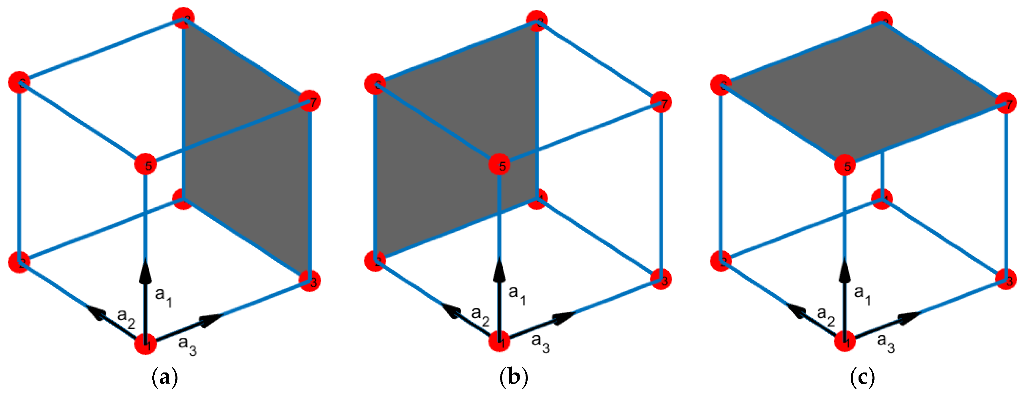
On the other hand, a crystallographic plane in a symmetrical lattice can be defined using the Miller indices in crystal Bravais lattices. Miller indices are defined by the planes intercepting along the unit cell axes. As shown in Figure 1, for example, the cubic cell has three crystallographic planes which can be numbered using Miller Indices Bravais system as (100), (010), and (001) [5].
In this paper, lattice unit cells are constructed by means of nodes and struts where a strut is a member that connects two nodes. Using the Bravais lattice terminology, a node in this paper is equivalent to a lattice point and is illustrated as a red point in Figure 2. Nodes occur at the intersections of one or more struts and a strut is a line or a member that is connected by two nodes. Crystallographic planes are defined when they can be drawn through a unit cell using only the nodes within that unit cell and that the resulting plane is either coplanar with the struts or intersects the nodes exclusively. A crystallographic plane may also be defined by symmetry elements within the unit cell if those planes pass through nodes.
The presented algorithm in this paper exploits the crystallographic planes by using them to connect cut struts where a cut strut is a section of the lattice inside a domain as illustrated in Figure 5.
While this can easily be expanded to all types of symmetries, the proposed meshing algorithm in this paper is only concerned with unit cells with translational or reflection symmetries. This limits the algorithm to work exclusively with cubic lattices from the Bravais lattice family [5]. However, cubic symmetries can be easily adapted for many other types of lattice symmetries. As shown in Figure 2, Cubic Bravais lattices have three topologies including the simple cubic or the primitive structure, the Body-Centered Cube (BCC), and the Face-Centered Cube (FCC). Symmetrical lattices that are also applicable for the presented lattice net algorithm include diamond and octet-truss topologies as they have Bravais cubic symmetry as well.
3. Trimmed Lattice with Conforming Net Algorithm Workflow
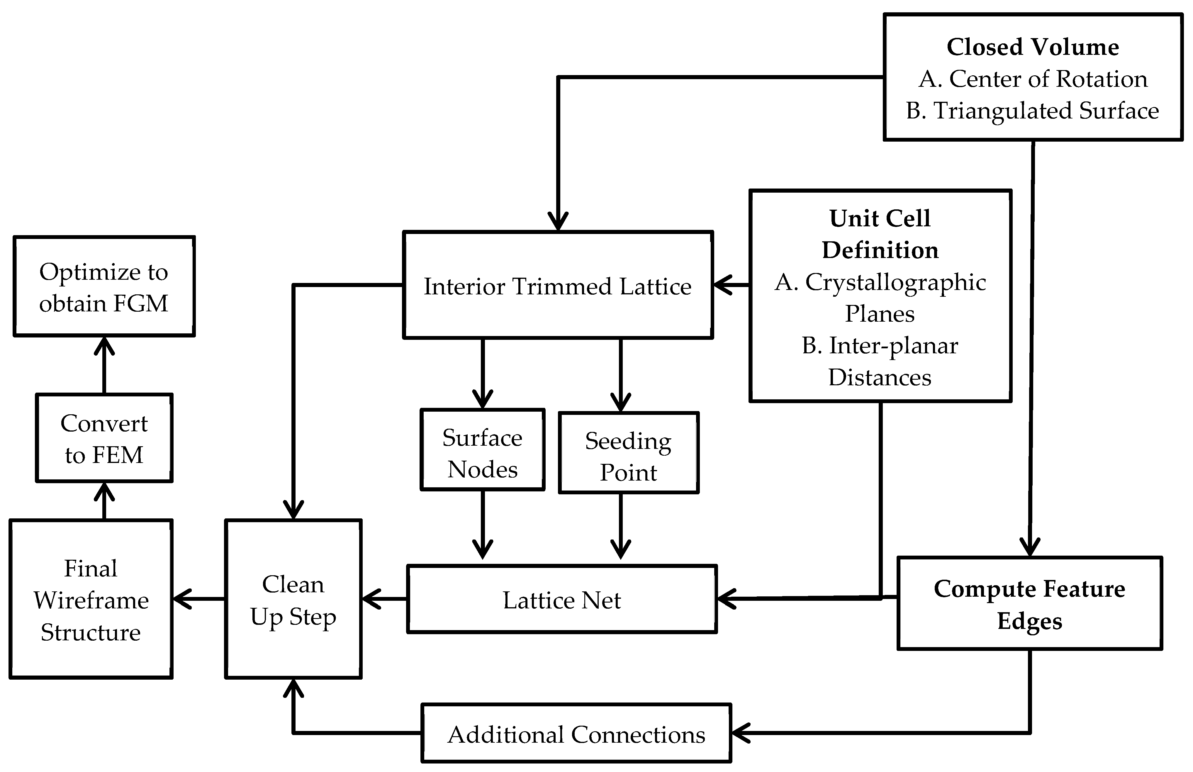
An interior trimmed lattice is a periodic structure that retains its periodicity within an arbitrary volume where the boundary of the volume does not influence the interior. A conforming net is a skin on the boundary of the trimmed lattice structure which connects the trimmed sections together in a mathematical or a logical pattern. The methodology for a conforming net (or lattice net) is presented to create a wireframe representation for symmetric unit cells of the Bravais family. The full workflow for generating a trimmed lattice with a conforming lattice net is presented in Figure 3. Each sub-algorithm is discussed in detail in the proceeding sections of this paper. The trimmed wireframe structure is then used for micro-truss optimizations to obtain functionally graded lattice materials.
4. Algorithm for an Interior Trimmed Lattice
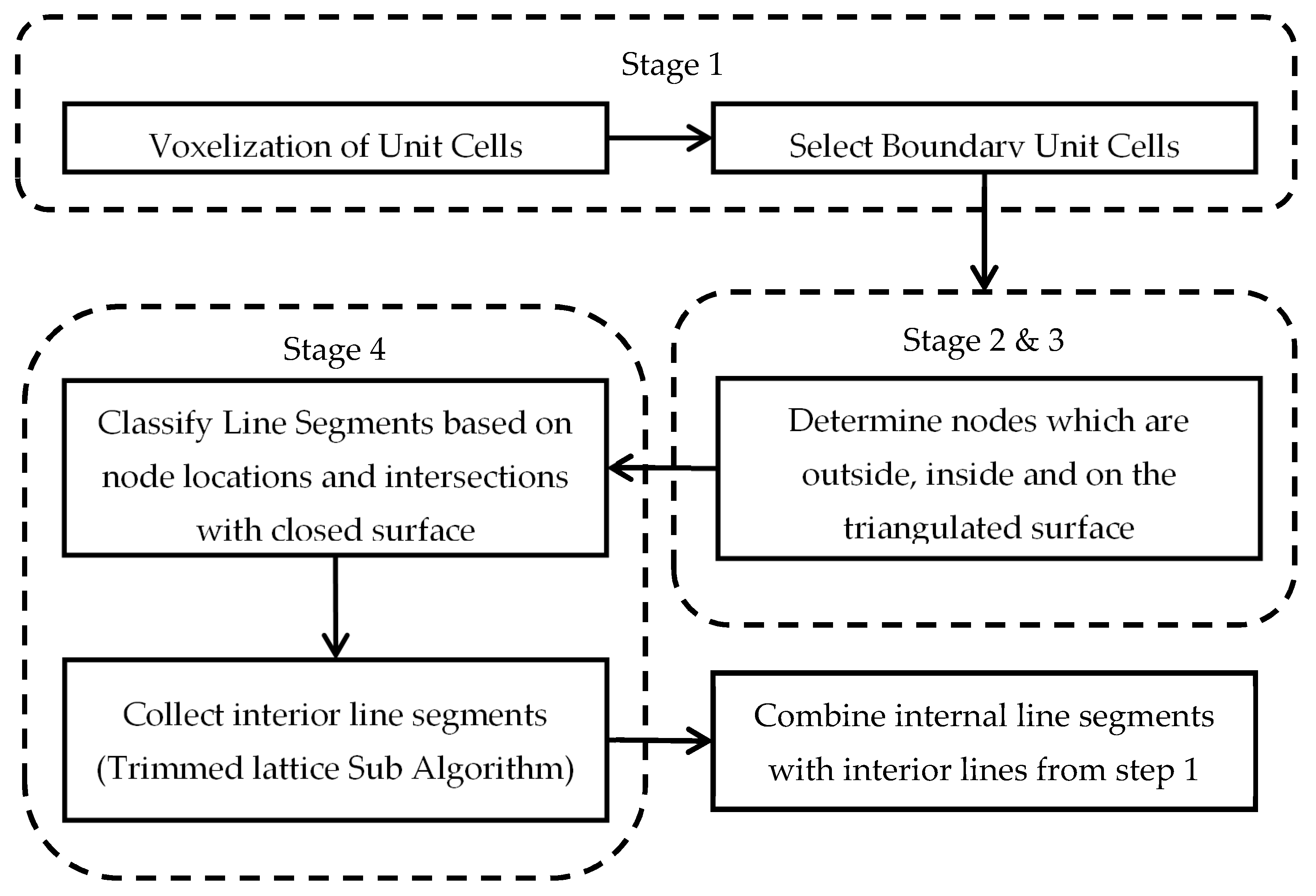
This section presents an algorithm for generating an interior wireframe structure of a trimmed lattice. The methodology implements the work of Tang et al. [8] but replaces a functional volume (FV) with a closed surface that is composed of triangles such as the CAD geometry presented in StereoLithography (StL) files [22], as shown in Figure 4; the algorithm includes four stages.
The first stage for creating the interior trimmed lattice replicates a lattice unit cell to fill a volume. This can be achieved through voxelization in a three-dimensional space [6]. The advantage of using voxels to fill a closed volume is that the boundary voxels can be extracted to be used in the trimming section of the algorithm. By limiting the number of struts to be processed by ignoring those which are fully inside, the volume increases the computational efficiency of the trimming algorithm. After trimming, the fully interior struts are combined with the cut struts to create the final trimmed lattice structure.
The second stage determines which nodes in the voxelated structure are outside or inside the closed surface. This is to group line segments based on the placement of the nodes in relation to the triangulated surface. The methods to sort the nodes are those formulated by Tuszynski [23] and Sven [24]. Ray-triangle intersection algorithms [25,26,27] determine if the point is interior or exterior of a closed surface. If an even number of ray intersection is found, then the point is outside of the surface, the point is outside the closed surface if an odd number is calculated.
Ray-triangle intersections can be determined by evaluating the intersection point between the ray and the plane given by the normal to the triangles. If the intersection point is expressed in terms of barycentric coordinates for that triangle, then it is possible to classify whether the ray intersects the triangle. In a mathematical sense, a ray with direction d and origin o intersects a triangle with edge vertices , , and if the following criteria shown in Equations (2) and (3) are satisfied:
where is the parametric distance along the ray and and are components of bary-centric coordinate system for a triangle. In practice, Cramer’s rule is used to solve for , , and [26]. Details of ray-search algorithms for interior/exterior point classification are shown in [12,13].
The third stage determines which nodes lay on the surface of the triangulated mesh. This stage is used for collecting information for classifying line segments in the fourth stage. Each node is projected onto the plane of each triangle and barycentric coordinates are used to check if the projected nodes lay within the triangles [14,15]. The criteria to determine if a node is within a triangle in three dimensions are
where is a function to determine if the node lies on a surface, is the first vertex of a triangle in , is the node being evaluated, is the unit normal of the triangle, is the numerical tolerance, and is the barycentric coordinates of a point for the triangle where is equal to
The fourth stage is the trimming algorithm which begins by evaluating each line segment from the voxelized structure and checks if an intersection occurs within it and the triangulated surface. Möller–Trumbore’s ray-triangle intersection algorithm is adopted for this operation [16,17]. During the trimming process, the nodes at the surface of the trimmed structure are also extracted to be used for constructing the lattice net.
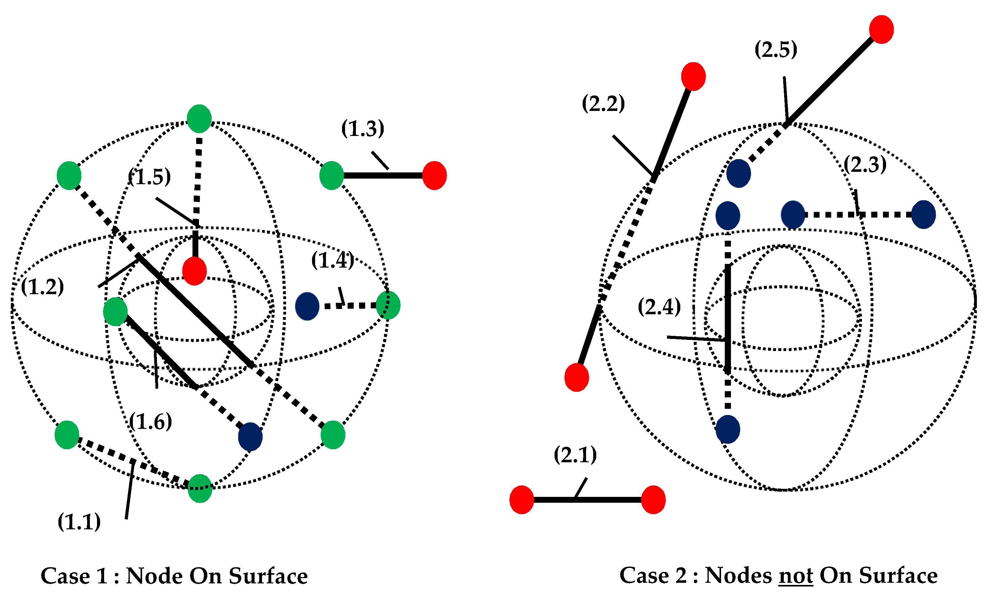
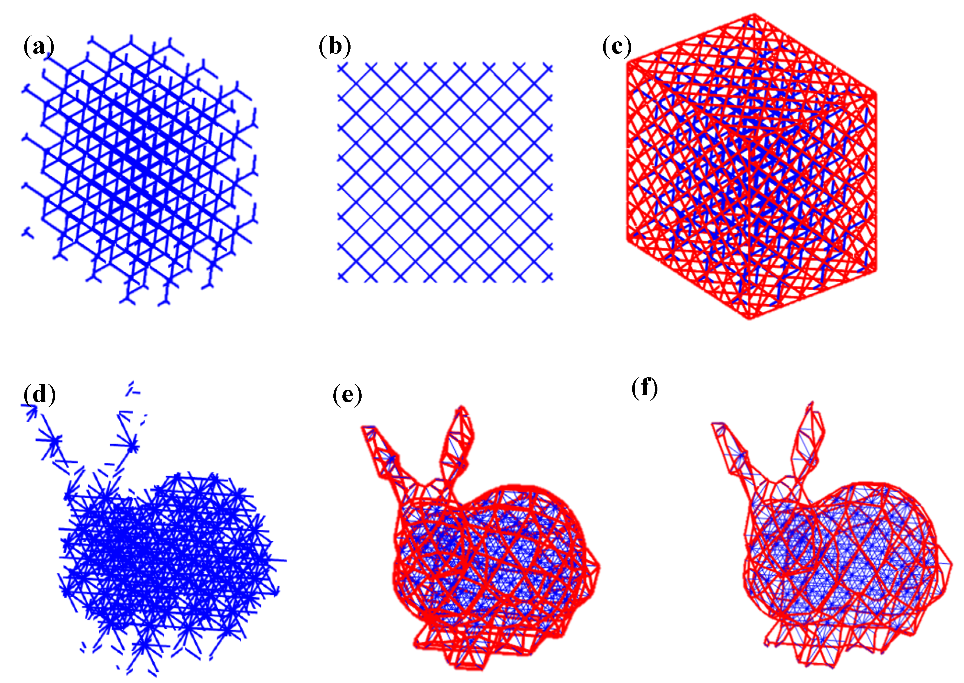
After calculating all possible intersections between the line and the triangulated surface, the algorithm is used to classify the intersections depending on the locations of the nodes from the second and third stage. The type of class determines if the line should be cut, kept, or rejected and which line segment pieces are to be retained. There are two main cases and eleven subcases for classifying line segments and is illustrated in Figure 5.
A hollow sphere is used to illustrate the different possibilities for a line segment intersection with a closed surface. Case 1 in Figure 5 shows six subcases where a node is on the surface of the triangulated surface while Case 2 contains five general subcases. The distinction between Case 1 and 2 is required because a node on the surface cannot be classified as either outside or inside the design space and the general method will fail. Dotted lines are line segments inside the hollow sphere and solid lines are located outside of the closed surface. The goal of the trimming and classification process is to retain the interior (dotted) line segments. The line subcase is used to determine a starting point (or reference node) for a pairing algorithm to determine the correct line segment pieces to be extracted. Intersection points at the surface are saved as surface nodes to build the lattice net.
Appendix A.1 contains Algorithm A1 that exploits line segments classification given positions of the nodes and its intersections with the triangulated surface. Algorithm A1 uses Boolean logical arrays to sort the line segments efficiently. After sorting, the interior line segment pieces can be identified by grouping nodes without replacement based on their distance from a reference node. In addition, Appendix A.2 presents the process of selecting the proper reference node for collecting the interior line segment pieces where a reference node is either an intersection point or an interior point depending on the line segment case. After the final step, the interior line segments are retained as the final trimmed lattices structure. The entire algorithm for generating the interior struts and collecting surface nodes is shown in Appendix A.3.
5. Algorithm for a Conformal Lattice Net for a Trimmed Symmetric Lattice
For a given closed surface and an interior trimmed lattice, it is possible to connect the cut struts together using the common crystallographic planes of the unit cell. Closing open connections is important, as unconnected struts bear no loads and only unnecessarily increase the weight and manufacturing time of the final design. Connecting the exterior lattice nodes also helps with ensuring that the entire volume is utilized.
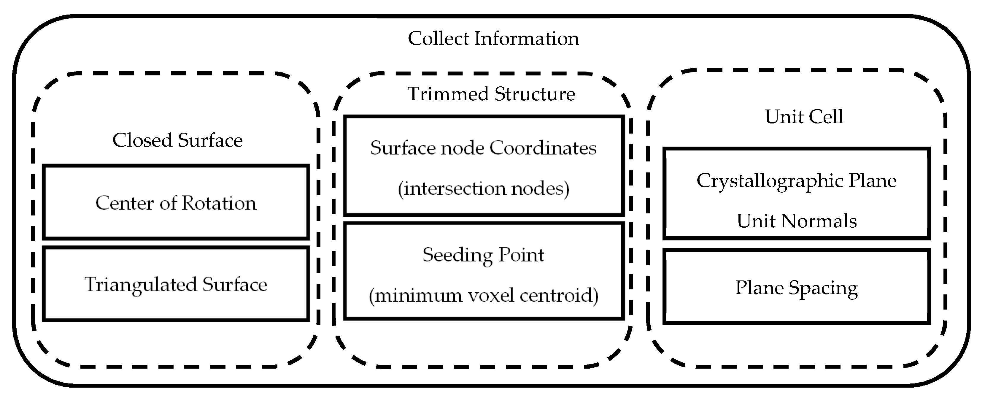
Before initializing the lattice net generation algorithm, the center of rotation (for the triangulated surface), surface node coordinates (intersection between the truncated struts and the triangulated surface), and a seeding point are required. The seeding point is the minimum coordinates for a unit cell or voxel centroid. The seeding point is used to orient and correctly space the contours along the triangulated surface. The center of rotation is used for plane-surface contour collection which rotates the triangulated surface so its z-axis is equivalent to the plane normal direction of the unit cells crystallographic planes. In addition, information about the unit cell crystallographic planes is required and includes the inter-planar spacing between common planes and their associated unit normal. Figure 6 displays and categorizes the necessary input required for the lattice net algorithm.
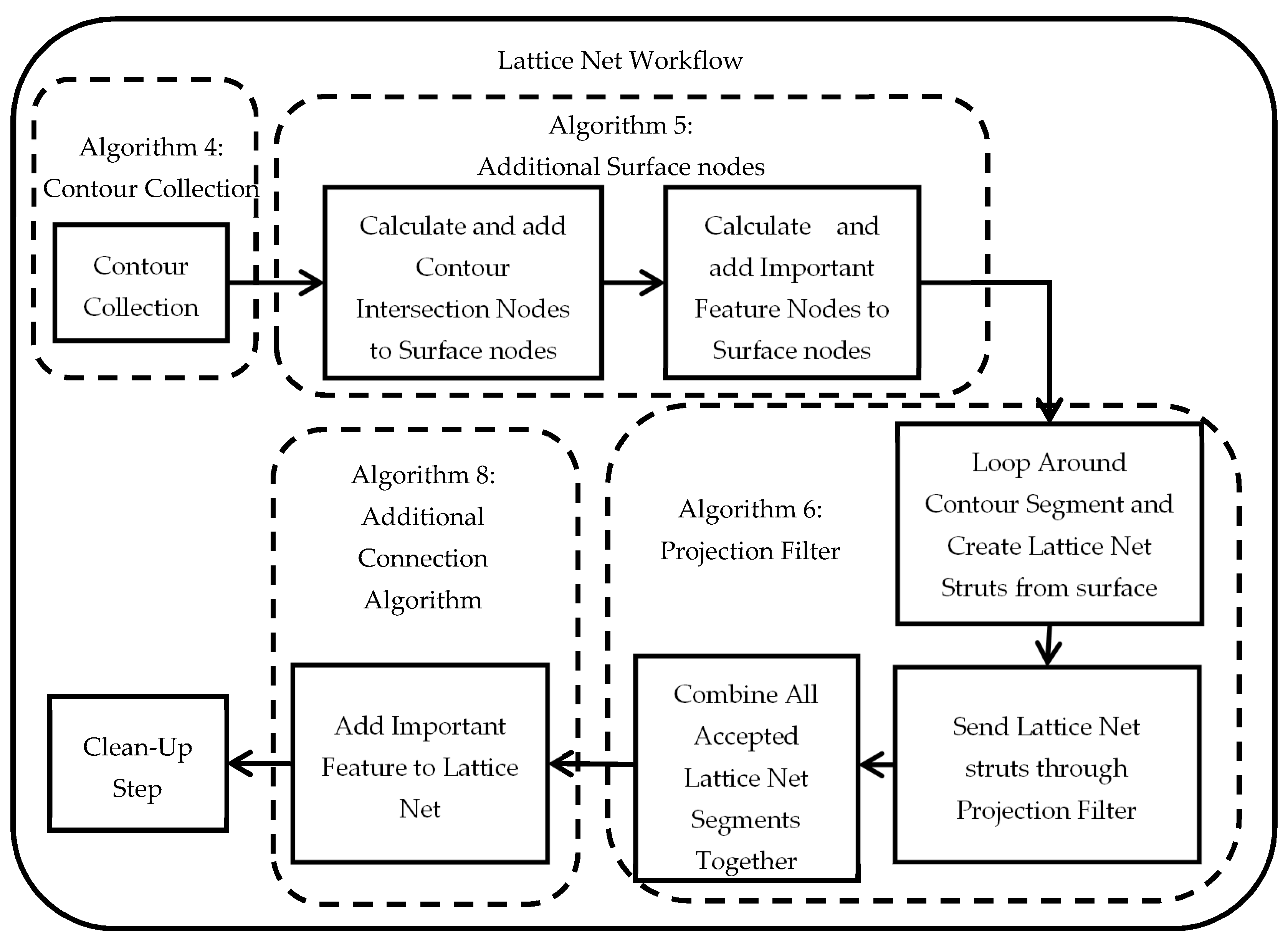
The lattice net generation algorithm contains five stages, as shown in Figure 7: a contour collection stage, additional nodes from contour intersection and “important features” collections stage, then the lattice net generations stage which includes a projection filter, then a feature preservation stage followed by a final clean-up stage. A feature is a sharp angle on the triangulated surface to be retained in the lattice net during the contour collection stage. After generating the lattice net, a postprocessing step is applied to remove any duplicate line segments. The final cleanup step, which collapses beams with less than three connections, is done to simplify the wireframe structure. A pseudocode is developed for the whole process and can be found in Appendix A.7.
5.1. Initial Contour Collection
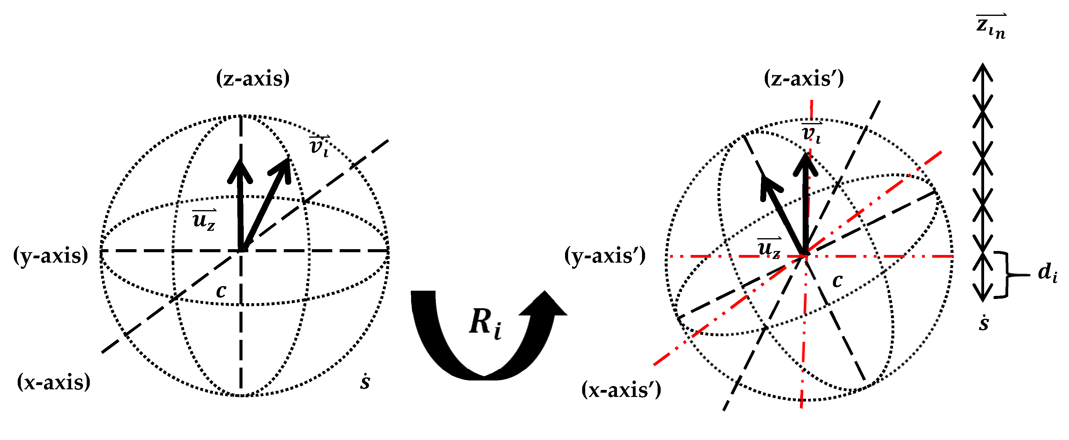
The first step collects the contours for all possible planes along the triangulated surface. The rotation center is used to rotate the triangulated surface so that the z-axis matches the normal of a particular crystallographic plane as illustrated in Figure 8. A rotation matrix is calculated for each crystallographic plane normal and can be defined as [28,29]
where is the rotation matrix to align with , is the identity matrix, is a skew-symmetric cross product matrix between , and and is a subscript for the crystallographic planes.
If both vectors and are equivalent, then the rotation matrix cannot be calculated and is instead replaced with the identity matrix. Another condition which results in a singular rotation matrix is when ; and must be replaced with . The vector is the crystallographic plane normal while is the direction of the z-axis and is .
Surface contours are collected at different elevations determined by crystallographic plane distances. The plane distances are the inter-planar distance between the same planes in a repeated unit cell structure. The planar elevations are calculated as
where is a sequence of elevations, is the inter-planar distance, and is the re-oriented seeding point for crystallographic plane . is an integer number such that the maximum elevation is higher than the rotated triangulated surfaces highest surface node. is the original coordinate of the seeding point and is the center of rotation.
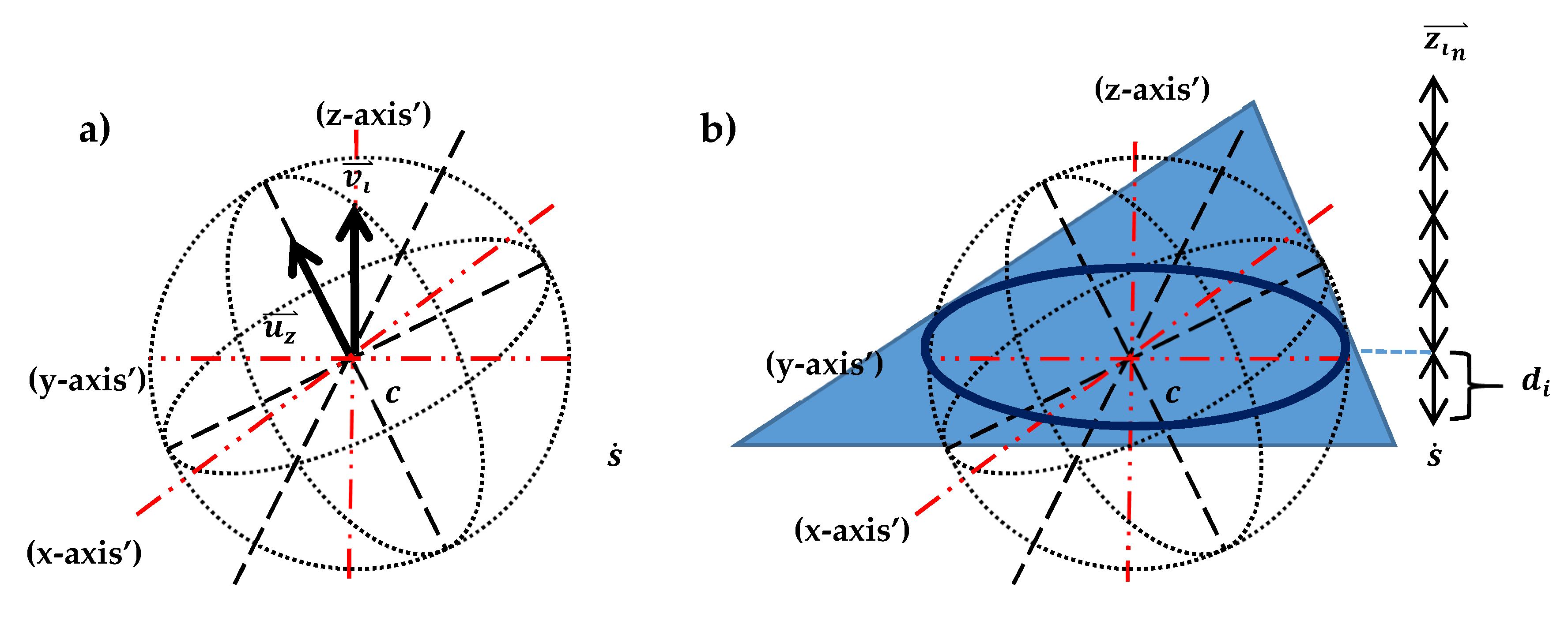
Contour edges are computed using the Möller–Trumbore’s algorithm for surface intersections [30,31]. As shown in Figure 9, one large equilateral triangle is used for slicing the triangulated surface; the contour edges are collected into organized lists to form a loop and then stored into an individual “bin” for each elevation and plane. For each contour, the nodes defining the path of the contour must be reoriented from the current z-axis to their original axis using about . A pseudocode for this process can be seen in Appendix A.4.
5.2. Additional Surface Nodes Calculations
Using the trimming algorithm, additional nodes are added to the input surface definition which are calculated from the intersections between the plane slicing contours. This occurs for lattice topologies such as BCC where an “X” shape of the interior struts must be projected onto the surface of the volume and can be seen in Figure 11a. In addition to the intersections, important sharp features can also be preserved. Important features can also be retained by supplying an edge list of sharp features. For example, the edges of a cube, shown in Figure 11b, are sharp features that can be preserved and retained in the lattice net. In MATLAB, this can be done using the function “featureEdges” [32].
The additional nodes for both the contour intersection and important features are found by first rotating the contour lines and the important feature edges around the center of rotation so that the crystallographic plane normal points into the z-direction. This rotation strategy is the same as for the contour collection algorithm shown in Equation (7). The second step is to calculate the intersection nodes from the specified planar heights for the given rotation. The heights or elevations are calculated using Equations (8) and (9). Edges in plane with the current plane or elevations are omitted. To find the intersection points, the feature and contour edges are converted into a parameterized line formulated as
where is the independent variable, and and are points along the line segment or edge. To solve for , Equation (10) can be rearranged as
where is a sequence of target elevations from the planar distances for a particular crystallographic plane . A valid intersection occurs when . Valid intersection points are rotated about with and added to the “bin” (or list) of surface nodes bin with duplicate nodes removed. This bin of nodes is then used to generate the lattice net in the third stage. A pseudocode is written to further explain the method and is referred to as “Appendix A.5. Algorithm A5: Additional Surface Nodes” in Appendix A.5.
5.3. Connecting the Lattice Net
The proposed algorithm loops through all the contours and connects the cut struts together based on a collection of surface nodes acquired from the second stage. Note in this research paper that the surface nodes obtained by the intersection points calculated from the trimming algorithm are the same as those calculated from the contour–contour intersection nodes. For this reason, it is possible to construct the net independently from the interior trimmed lattice.
For a collection of contours for a specific crystallographic plane (), the lattice net generation algorithm collects any surface nodes that lie within the specified contour loop into a list. That list is then converted into new line segments that represent wireframe sections of the lattice net.
When all the contours have been evaluated for the current plane, a projection filter is used to remove line segments that do not satisfy the unit cells strut orientation for that crystallographic plane. The filter also aims to remove zero-length line segments when projected into specific planes. If a line segment is accepted by the filter at certain angles, then it is retained in the lattice net. An illustration of this procedure can be seen in Figure 10a for a BCC lattice. The red segments are the accepted sections from the filter while the black sections are the rejected pieces. The summation of all the accepted contour sections will create the final lattice net. An example of the final lattice net and its construction is shown in Figure 10c.
There are two possible filtering methods developed in this work. The first filter works by comparing the ratio of the projected normalized crystallographic plane normal into the x, y, and z planes with the projected length of the line segments normalized directions into the same x, y, and z planes. However, any projection plane can be used depending on the type of lattice topology or crystallographic family. Projection of a line onto a plane can be calculated as
where is the normalized direction of the line, is the plane unit normal, and is the resulting projected line. For both discussed filters in the paper, the projected normal of the crystallographic plane is projected along with the list of line segments.
If the line segment can satisfy the projection onto any of the three planes, then it is not rejected. A tolerance is given for the ratios to relax the acceptance criteria; a tighter tolerance would mean that the remaining line segments will need to strictly satisfy the projection lines. A tolerance of zero would work best if the curvature of the surface is zero such as a cube. For curved surface a higher tolerance is needed. Equation (13) is used to determine if a line segment will be accepted by the first filter.
where is the projected crystallographic plane normal onto the projection plane, is a projected line segment onto the projection plane, and is a tolerance level.
The second projection filter method compares the components of the projected segments to and as the filtering criterion. The criteria to determine if the line segment is accepted by the second filter type can be expressed as
where indexes the dimensional entries of the vectors.
The second filter type cannot be applied to cubic unit cell crystallographic planes (100), (010), and (001) because all line segments will be rejected. However, this method has shown to work very well with BCC unit cell topologies for planes (110), (101), and (011). The pseudocode for the projection filters is given in Appendix A.6.
5.4. Additional Connections for the Conformal Lattice Net
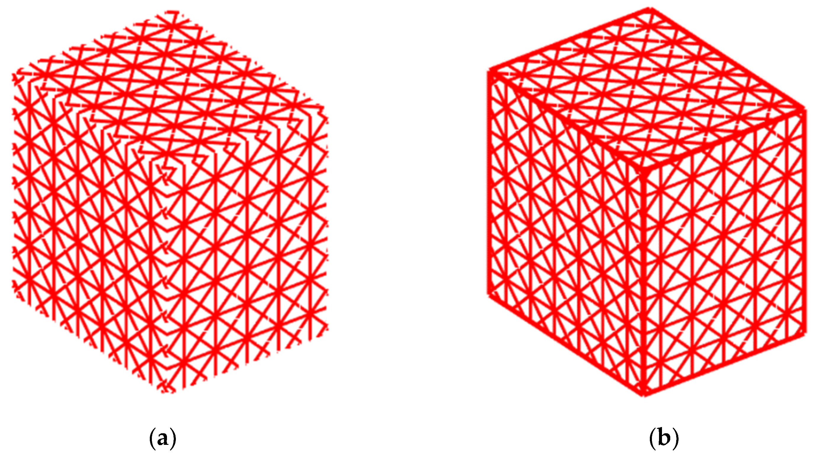
After the initial construction of the lattice net, unit cells could be projected onto sharp corners or features. If the unit cell size does not precisely match the dimensions of the sharp geometries, a discontinuity between the struts will occur at the sharp feature. This occurs when the corner of a unit cell is not placed directly at a vertex. Figure 11a shows a cube without any additional connections at the edges, while Figure 11b shows the addition of the important features into the lattice net. The added features allow structural loads to be transferred uniformly throughout the net eliminating discontinuities and improving the mechanical behavior of the lattice structure.
To promote better continuity in the lattice structure, sharp features of the geometry are extracted and added to the lattice net. This is done by collecting sharp edges of the input triangulated surface and then organizing those edges into open and closed loops. Loops are defined as edges connected to other edges based on a common node. A closed loop is a sequence of nodes where the first and final nodes are identical while an open loop has different nodes at each end. The nodes at intersections or junctions between the open and closed loops are also identified and are added to the list of lattice nodes. Junction points are found if a node is referenced more than twice from the extracted edges.
The new struts are created by following the open and closed loops and collecting any of the lattice net nodes or junction points that fall within the edges into an ordered list or sequence. If each node in the ordered lists is given unique identification, then the new struts can be created by connecting the nodes together from their positions in a list. A pseudocode is for the process is found in Appendix A.8, labeled as “Appendix A.8. Algorithm A8: Additional Connections Algorithm” to explain the entire process.
5.5. Clean Up Step
The last step for the wireframe development includes a clean-up stage. Line segment connections are simplified by ensuring that all nodes are connected to at least three line segments. This does not include nodes that are used to conserve important features or sharp edges. After the net clean-up step, the interior trimmed lattice and lattice net are combined, and any duplicate line segments are removed from the structure. In a structural sense, the clean-up step helps improve connectivity by removing non-load-bearing connections and creates more efficient load paths.
6. Numerical Examples and Demonstrations
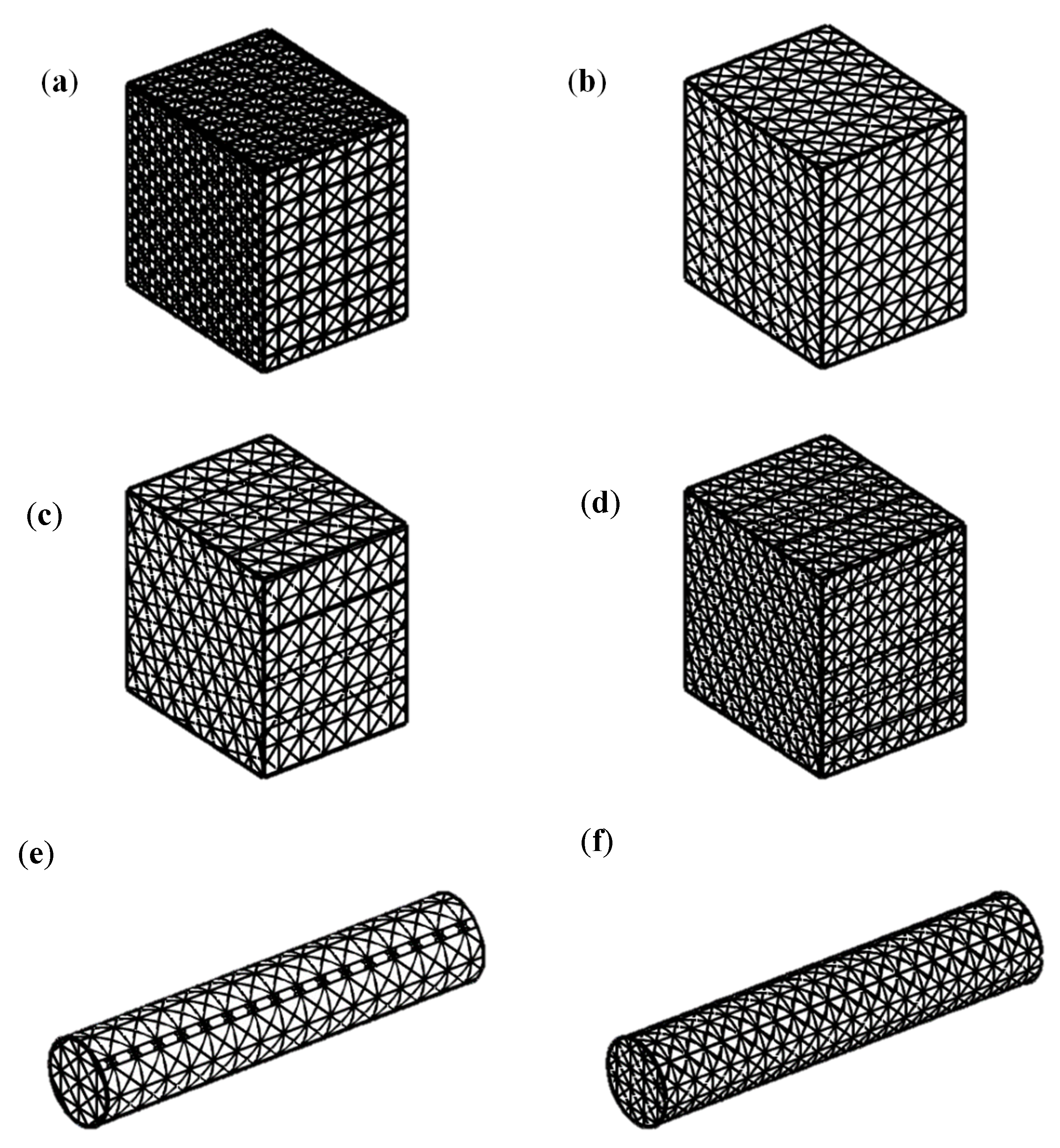
The importance of filtering the struts is shown in Figure 12a,b. The initial surface contours create additional vertical cuts in Figure 12a on the front and top faces. Figure 12b is the result of projection filtering to remove the unneeded contour lines. The effects of scaling by different unit cell sizes are shown in Figure 12e,f. The cylinder in Figure 12e contains small patterns where the unit cell is cut and produces nonuniform geometry radially. Figure 12f shows for smaller unit cell sizes the effects nonuniformity is diminished. Rotation of different sized unit cells is demonstrated in Figure 12c,d where the front faces pattern is rotated 30 degrees and has a net pattern slightly smaller than the top and side faces.
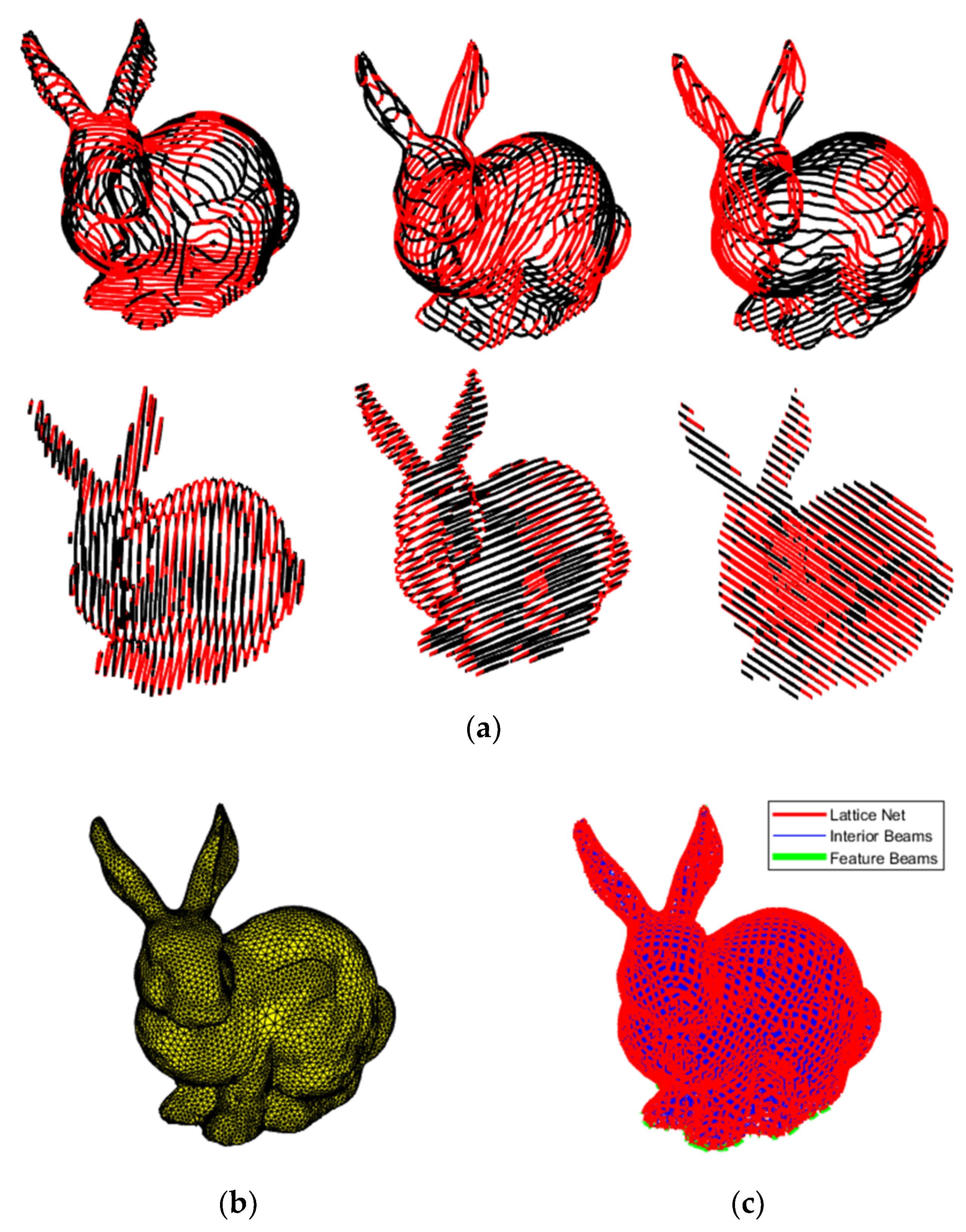
Six crystallographic planes are observed in cubic Bravais lattices. FCC topology contains six plane types and is a superposition of the Cubic planes and the BCC planes. For some lattice configurations such as diamond (Figure 13a) and the octet truss (Figure 13d), the side profiles of these topologies are equivalent to the BCC and FCC unit cell, respectively. Figure 13b shows the front view of the diamond lattice is equivalent to that of the BCC lattice and its skin is meshed using crystallographic planes (110), (101), and (011) in Figure 13c.
Figure 13f displays a lattice net around the Stanford bunny model using only three crystallographic planes and no filter to connect an interior octet-truss lattice shown in Figure 13d. The resulting net is very similar to Figure 13e which had used all family planes from {111} and the projection filter. This shows the possibility to omit the filter and select a few planes of symmetry to connect all the cut struts together of a trimmed lattice.
7. Lattice Net Case Study Example for Engineering Applications
The purpose the lattice trimming algorithm is to generate a wireframe structure that can be embedded into any complex geometry. This wire frame geometry is then directly converted into a collection of beam elements in a finite element mesh for sizing optimizations. This section will demonstrate the performance of an optimized lattice structure meshed with different lattice topologies when a lattice net is or is not applied to the outside geometry. A simple Messerschmitt–Bolkow–Blohm (MBB) Beam [33] is used to compare the different lattice topologies and their performances when subjected to sizing optimizations.
7.1. Problem Formulation
The optimization problem is formulated such that design variables are the cross section radii of the beam elements and are named and seen in Equation (15). Tapered beams are used in the finite element mesh with the common joints as a unified design variable for all connected tapered beams. The advantage of using tapered beam elements is that the unified joints will reduce the number of design variables during the optimization. The optimization problem will be referred to as a lattice beam optimization and is described by Equation (15).
where is the cross-sectional radii of the ends of the tapered beams, KI is the global stiffness matrix as a function of the design variables, F is a constant force vector for static analysis, is the maximum allowable stress (880 MPa), is the density of the material, is the length of the ith beam, and is the number of tapered beam elements. The objective measures the mass. The minimum radii distance for the optimization is 0.001 mm and the maximum radius is 0.5 mm. Titanium was chosen as the material of choice and the young’s modulus is rated at 11,400 MPa, Poisson ratio is 0.31, density is 4.506 g/cm3, and has a yield strength of 880 MPa. As a note to the reader, buckling is traditionally considered in beam sizing optimizations but is omitted due to limitations in the structural solver [34]. The effectiveness of the lattice net in this research will therefore demonstrate the benefits for stress constraint mass minimization.
The MBB beam is meshed with different lattice topologies and includes Cubic, BCC, FCC, and the octet truss. The MBB beam is a double supported beam with a vertical force applied at the center. Figure 14 shows the MBB mesh where the yellow elements represent the lattice domain to be replaced with a trimmed lattice structure and the brown elements represent the solid domain to attach forces and boundary conditions.
The beams are then attached to the solid elements by tie contacts (contact surface), where the lattice beam nodes are the slave set and the solid elements as the master set. For test cases with a lattice net, any beam elements whose nodes are twice connected to the master set are removed. The optimizations for the case study will be done in Altair Optistruct using the “BIGOPT” optimization algorithm [34].
The dimensions of the MBB beam are 20 mm in the x direction, 10 mm in the y direction, and 120 mm in the z direction. The boundary conditions are applied such that the side of the beam where the applied force is placed is free to move in the x-direction. The constraints applied on the side of the beam without applied loads are free to move in the z-direction. The applied force is 500 N in the x-direction and will cause a maximum deflection of 0.0215 mm in the x-direction with a maximum von Mises stress of approximately 21 MPa.
7.2. Results
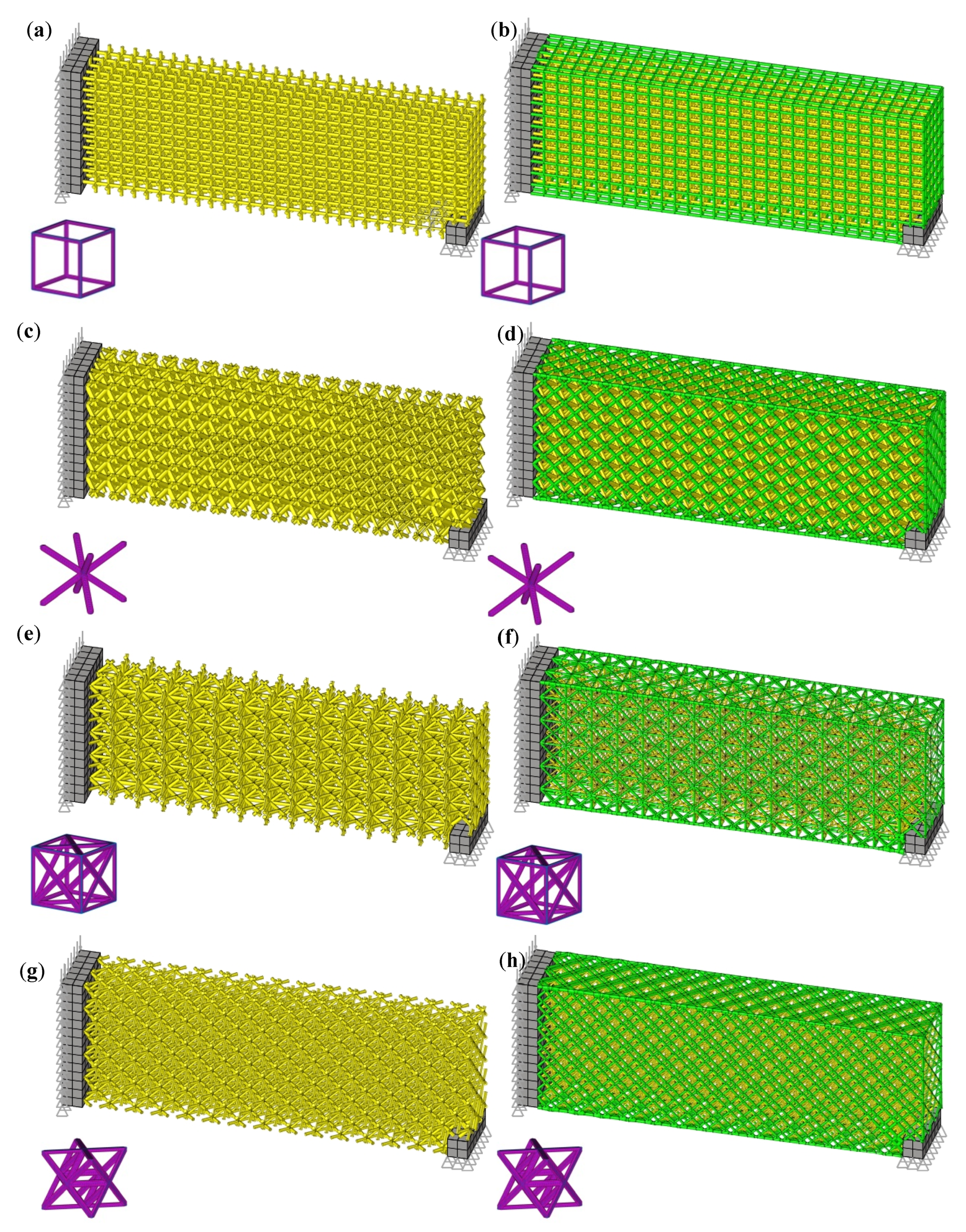
The results in Table 2 show that when a lattice net is added to the outside of a trimmed lattice structure, the optimizations with the net had a significantly lower final mass. This indicates that an added exterior lattice net is beneficial when creating lattice embedded geometries for trimmed lattices. A lower mass will therefore reduce printing time and save on material costs.
The topology with the lowest mass was the FCC topology. This could be a result of it having more favorable strut directions and connections and a larger unit cell size than the other topologies for this specific load case. The maximum stress in the FCC final design was also much lower than the constraint maximum, meaning that the final mass could potentially be much lower. Figure 15 displays the final optimized designs; the beam size distribution was fairly homogenous among the test cases and the majority of the beam’s radii fell between 0.24 and 0.26 mm. The specific stiffness for the net-based optimization cases where much higher than those without the net. The octet truss, however, had decreased its specific stiffness as the results of adding the lattice net. However, specific strength had improved significantly for all cases from the addition of the lattice net.
The optimization problem posed assumes that the maximum stress in the beams does not exceed the yield strength of the material. Realistically, the maximum stress in the beams is not the highest stress seen by the complex structure but at the nodes connecting the struts together where stress concentrations are located. Current Euler beam theory cannot capture this phenomenon and incorporate it into the optimization process. This in turn resulted in lighter final designs than required for the desired loads. To avoid potential stress concentrations with Euler beams, a stricter stress constraint would need to be imposed or by applying a new beam formulation specifically for lattice struts. Some research has been attempted to create a new element type to more accurately model lattice struts and could take into consideration of the stress concentrations at the nodes [35,36]. As the methods for representing lattice struts improve, so can the application of beam optimizations on wireframe lattice structures.
8. Advantages and Disadvantages of the Current Lattice Net Algorithm
The main advantage of the lattice net algorithm is its ability to connect the struts of a symmetric unit cell of any size while maintaining the overall geometry of the triangulated surface. The ability to preserve important features is another advantage which helps promote continuity and shape. The lattice net construction is also very fast, even for a high number of surface nodes and plane intersections. Another crucial advantage is that connectivity is guaranteed among all cut struts, even if the lattice net does not follow the unit cell pattern very well. The final wireframe is also memory-efficient due to being comprised of a list of nodal coordinates and can be easily converted into a finite element mesh for optimization applications. Another key factor about the lattice net algorithm is that its creation is independent of the interior trimmed lattice. This is because all of the contour intersections between different crystallographic planes produce the same intersection points from the lattice trimming section. The final advantage is that a BCC combined with a CUBIC lattice net can be used for many lattice topologies that share cubic symmetries such as the diamond lattice.
Disadvantages include the lack of support for non-symmetric lattices. Truncated octahedron lattice structures cannot be used for the lattice net to accurately capture the projected pattern of the lattice on a surface. However, a BCC and cubic lattice net can connect all the cut struts of this topology because it contains Bravais crystallographic planes. A final disadvantage is that it is not robust and depends on the tolerance level of the projection filter. For complex surfaces, the projection filter may fail to filter out or over filter connected struts. At sharp curvatures, the connected struts for the net may be rejected more easily by the filter. There is also an issue of impossible strut connections at highly curved cross sections. The issue of projection onto curved surfaces for lattice nets has been noted by Aremu et al. [6] in their own implementation of conforming lattice skins. Irregular strut connections arise from complex geometries such as saddle points which give the algorithm the most problems. However, for flat surfaces, such as a cube or rectangle, the algorithm works very well as seen Figure 11.
In conclusion, the lattice net algorithm, while not perfect, is quite flexible as only two or three crystallographic planes are needed to connect all the cut struts together for most symmetric topologies as seen in Figure 13f.
9. Conclusions
A method for creating a trimmed wireframe lattice was developed. This method provides a list of surface nodes from the trimming operation to be used for constructing the lattice net. In addition, a novel method for constructing a conformal lattice net as a wireframe is presented. The generated lattice net is created by using the crystallographic planes from symmetric unit cell topologies. The lattice net algorithm functions by using contours from plane slicing at calculated intervals to connect surface nodes together which are then paired up and converted into struts. A projection filter is applied to remove unneeded connections and produce an approximate projection of the unit cell onto a closed triangulated surface. The proposed algorithm can produce a net for any complex geometry, and construction of the net is independent of the interior trimmed structure.
An engineering comparison for microscale optimization of functionally graded materials with and without lattice nets was also done. For topologies such as cubic, BCC, and FCC, the addition of a lattice net was beneficial during the micro-scale optimizations. The FCC topology performed best with the net as it required the least mass for the optimization load case. The performance improvement of the added net shows that the overall mass of the lattice structure was lower and yielded higher specific strength and stiffness.
Author Contributions
Conceptualization, M.S.A.E.; methodology, E.T. and M.S.A.E.; software, E.T.; validation, E.T. and M.S.A.E.; formal analysis, E.T.; investigation, E.T. and M.S.A.E.; resources, M.S.A.E.; data curation, E.T.; writing—original draft preparation, E.T.; writing—review and editing, M.S.A.E.; visualization, E.T.; supervision, M.S.A.E.; project administration, M.S.A.E.; funding acquisition, M.S.A.E. Both authors have read and agreed to the published version of the manuscript.
Funding
This research was funded by BOMBARDIER INC., in collaboration with CARIC National Forum, grant number MDO-1601 TRL4+ and MITACS Canada, grant number IT07461.
Institutional Review Board Statement
Not applicable.
Data Availability Statement
The data presented in this study are available on request from the corresponding author.
Acknowledgments
The authors would like to thank the financial support from BOMBARDIER INC. Montreal, in collaboration with CARIC National Forum and MITACS Canada.
Conflicts of Interest
The authors declare no conflict of interest.
Appendix A
Appendix A.1. Algorithm A1: Trimmed Lattice Case Sorting
| Algorithm A1: Trimmed Lattice Case Sorting |
| {case_select, in_t, surf_t} = AlgortithmA1(in, surf, nodal_ids, int_crd) |
| Input: in: A logical array that classifies nodes as inside the volume |
| surf_t: A logical array classifying nodes as on the surface |
| int_crd: A list of intersection points |
| nodal_ids: A line segment as a pair of nodal ids |
| Output: a logical array to select the case case_select, in_t and surf_t |
| 1. Index in and surf using the nodal ids to create in_t and surf_t |
| 2. Get logical: int_occur is true if int_crd contains intersection points |
| 3. Get logical: C1A = surf_t[1] ∧ in_t[2] |
| 4. Get logical: C1B = surf_t[2] ∧ in_t[1] |
| 5. Get logical: C1C = surf_t[1] ∧ ¬in_t[2] |
| 6. Get logical: C1D = surf_t[2] ∧ ¬in_t[1] |
| 7. Get logical: dual_surf = surf_t[1] ∧ surf_t[2] |
| 8. Get logical: single_surf = (surf_t[1] ∧ ¬surf_t[2]) ∨ (¬surf_t[1] ∧ surf_t[2]) |
| 9. Get logical: no_surf = ¬surf_t[1] ∧ ¬surf_t[2] |
| 10. Get logical: both_interior = in_t[1] ∧ in_t[2] |
| 11. Get logical: both_exterior = ¬in_t[1] ∧ ¬in_t[2] |
| 12. Case1.1: case_select[1] = dual_surf ∧ ¬int_occur |
| 13. Case1.2: case_select[2] = dual_surf ∧ int_occur |
| 14. Case1.3: case_select[3] = single_surf ∧ (C1C ∨ C1D) ∧ ¬int_occur |
| 15. Case1.4: case_select[4] = single_surf ∧ (C1A ∨ C1B) ∧ ¬int_occur |
| 16. Case1.5: case_select[5] = single_surf ∧ (C1C ∨ C1D) ∧ int_occur |
| 17. Case1.6: case_select[6] = single_surf ∧ (C1A ∨ C1B) ∧ int_occur |
| 18. Case2.1: case_select[7] = no_surf ∧ both_exterior ∧ ¬int_occur |
| 19. Case2.2: case_select[8] = no_surf ∧ both_exterior ∧ int_occur |
| 20. Case2.3: case_select[9] = no_surf ∧ both_interior ∧ ¬int_occur |
| 21. Case2.4: case_select[10] = no_surf ∧ both_interior ∧ int_occur |
| 22. Case2.5: case_select[11] = no_surf ∧ single_surf ∧ int_occur |
| ∨ = Or, ∧ = And, ¬ = not. |
Appendix A.2. Algorithm A2: Trimmed Lattice Sub Algorithm
| Algorithm A2: Trimmed Lattice Sub-Algorithm |
| {tmp_mat_sort, surf_nodes} = AlgorithmA2(case_select, in_t, surf_t, nodal_ids, int_crd) |
| Input:case_select: A logical array to select the case (or string) |
| nodal_ids: A line segment as a pair of nodal ids and coordinates |
| int_crd: list of nodes from intersection between surface FV and a line segment |
| in_t, surf_t |
| Output: An organized list tmp_mat_sort, a list of nodes at the surface surf_nodes |
| 1. Organize all intersection points and nodes into a list starting from the closest to the first node referenced by the line segment (index = 1) |
| 2. switch (case_select) |
| 3. Case 1.3 ∨ Case 2.1 |
| 4. Reject the Line, set tmp_mat_sort as empty |
| 5. Case 1.1 ∨ Case 1.4 ∨ Case 2.3 |
| 6. Accept the Line and save both nodes to surf_nodes |
| 7. Case 1.2 |
| 8. Save both nodes to surf_nodes |
| 9. Case 1.5 |
| 10. If surf_t[2] then |
| 11. Flip tmp_mat_sort |
| 12. Save node 2 to surf_nodes |
| 13. else |
| 14. Save node 1 to surf_nodes |
| 15. end if statement |
| 16. Remove the last row of tmp_mat_sort |
| 17. Case 1.6 |
| 18. If surf_t[2] then |
| 19. Flip tmp_mat_sort |
| 20. Save node 2 to surf_nodes |
| 21. else |
| 22. Save node 1 to surf_nodes |
| 23. end if statement |
| 24. if (tmp_mat_sort has an odd number of points) then |
| 25. Remove the surface node from the list |
| 26. end if statement |
| 27. Case 2.2 |
| 28. Remove the first and last rows from tmp_mat_sort |
| 29. Save the intersection nodes to surf_nodes |
| 30. Case 2.4 |
| 31. Pair up new beams using tmp_mat_sort. |
| 32. Save the intersection nodes to surf_nodes |
| 33. Case 2.5 |
| 34. If in_t[2] then |
| 35. Flip tmp_mat_sort |
| 36. end if statement |
| 37. Save the intersection nodes to surf_nodes |
| 38. Remove the last row from tmp_mat_sort |
| 39. End case statement |
| 40. Pair up new beams using tmp_mat_sort |
Appendix A.3. Algorithm A3: Trimmed Lattice Algorithm
| Algorithm A3: Trimmed Lattice Algorithm |
| { lattice_nodes, interior_lattice, surf_nodes_total } = AlgorithmA3(unit_cell, FV) |
| Input: unit_cell: type and size |
| A closed triangulated surface FV |
| Output: trimmed lattice nodes lattice_nodes, connectivity table interior_lattice and surf_nodes_total |
| 1. Voxelate the closed Surface FV with lattice unit cells |
| 2. Select the boundary voxels (unit cells) and save the interior as a separate object |
| 3. Classify nodes as inside the volume (in) or as a surface node (surf). |
| 4. Initialize a surf_nodes_total, interior_lattice and lattice_nodes bin |
| 5. For each (line segment in the boundary voxels) then |
| 6. Compute intersections between FV and the current line segment as int_crd |
| 7. {case_select, in_t, surf_t} = AlgortithmA2(in, surf, nodal_ids, int_crd) |
| 8. {tmp_mat_sort, surf_nodes} = AlgorithmA3(case_select, in_t, surf_t, nodal_ids, int_crd) |
| 9. Add surf_nodes to surf_nodes_total and lattice_nodes |
| 10. Add tmp_mat_sort to interior_lattice |
| 11. End For loop |
| 12. Combine interior_lattice with the interior voxel unit cells |
Appendix A.4. Algorithm A4: Contour Collection
| Algorithm A4: Contour Collection |
| {contour_bin, edge_nodes} = AlgorithmA4(seeding_point, FV, unit_cell) |
| Input: unit_cell: crystallographic planes and planar distances |
| A closed triangulated surface FV and center of rotation c |
| The minimum coordinates from voxel centroids seeding_point |
| Output: contours bin called contour_bin and a set of nodes called edge_nodes |
| 1. Initialize contour_bin to store results for each crystallographic plane |
| 2. For each (crystallographic plane) then |
| 3. j = j + 1 |
| 4. Rotate FV and seeding_point around c so the current plane normal points in the z-axis. |
| 5. Beginning from the seed point elevation, calculate elevations (distance between elevation points are the inter-planar spacing). |
| 6. Calculate the number of elevations num_elev |
| 7. Create a sub bin surface_intersection for each elevation |
| 8. For i = 1 to num_elev then |
| 9. Perform surface intersection calculation at the given elevation and |
| save the result into surface_intersection[i] |
| 10. Rotate the intersection nodes back to the original orientation and |
| add them to edge_nodes |
| 11. Process edges or triangles on the cutting plane separately then add |
| the contour edges into surface_intersection[i] |
| 12. Organize surface_intersection[i] into closed loops |
| 13. End For Loop |
| 14. Add surface_intersection to contour_bin[j] |
| 15. End For Loop |
Appendix A.5. Algorithm A5: Additional Surface Nodes
| Algorithm A5: Additional Surface Nodes |
| {new_surface_nodes} = AlgorithmA5(feature_edges, feature_nodes, contour_bin, edge_nodes, seeding_point, rot,unit_cell) |
| Input: Feature edges feature_edges and the associated nodes feature_nodes |
| unit_cell: crystallographic planes and inter-planar distances |
| contour_bin, edge_nodes, seeding_point, rot |
| Output: a list of new surface nodes new_surface_nodes |
| 1. Initialize new_surface_nodes |
| 2. For each (crystallographic plane) then |
| 3. j = j + 1 |
| 4. Rotate FV, seeding_point, feature_nodes and edge_nodes around rot so the current plane normal points in the z-axis. |
| 5. Create list of edges from contour_bin[j] and feature_edges |
| 6. Omit all edges in plane with the current crystallographic plane |
| 7. Beginning from the seed point elevation, calculate elevations (distance between elevation points are the inter-planar spacing). |
| 8. Create parameterized line equations for the edges (Equation (1)) |
| 9. Given the elevations as planes, apply Equation (2) to calculate the intersection points |
| 10. Rotate the intersection points back by applying the inverse rotation |
| 11. Add the new points to new_surface_nodes |
| 12. End For Loop |
Appendix A.6. Algorithm A6: Projection Filter
| Algorithm A6: Projection Filter |
| {lattice_net_new} = AlgorithmA6(lattice_net_in, surface_nodes, Proj_norms, Cryst_plane, filter_type, tolerance) |
| Input: list of lattice struts lattice_net_in and surface_nodes for a crystallographic plane |
| Proj_norms: A set of projection plane normals (ex: xy, xz, zy) |
| A filter_type {1 or 2} and tolerance setting tolerance |
| Cryst_plane: crystallographic plane |
| Output: an filtered list of lattice struts lattice_net_new |
| 1. Initialize lattice_net_new |
| 2. For each (projection plane) then |
| 3. Project normal of Cryst_plane onto the projection plane to make p_proj |
| 4. Project lattice_net_in onto the projection plane to make lattice_net_proj |
| 5. switch (filter_type) |
| 6. case 1 |
| 7. Compute ratios between the projected lengths of |
| lattice_net_proj to p_proj |
| 8. Add line segments where the ratio is within tolerance to |
| lattice_net_new |
| 9. case 2 |
| 10. If (crystallographic plane is in the xy,xz or yz plane) then |
| 11. Add all line segments into lattice_net_new |
| 12. Else |
| 13. Compute and calculate ratios of the directions |
| between lattice_net_proj to p_proj |
| 14. Add line segments where the ratios are within |
| tolerance to lattice_net_new |
| 15. End If Statement |
| 16. end switch statement |
| 17. End For Loop |
Appendix A.7. Algorithm A7: Lattice Net
| Algorithm A7: Lattice Net |
| {lattice_net, lattice_net_nodes} = AlgorithmA7(unit_cell, c, FV, surf_nodes_total) |
| Input: unit_cell: crystallographic planes and inter-planar distances |
| c, FV, surf_nodes_total, filter_type, tolerance |
| Output: list of lattice struts for the lattice net lattice_netand nodes lattice_net_nodes |
| 1. Initialize lattice_net |
| 2. { contour_bin, edge_nodes } = Algorithm5(seeding_point, FV, unit_cell) |
| 3. { new_surface_nodes } = Algorithm6(feature_edges, feature_nodes, contour_bin, edge_nodes, seeding_point, rot,unit_cell) |
| 4. Add new_surface_nodes to surf_nodes_total |
| 5. For each (crystallographic plane in Cryst_plane) then |
| 6. j = j +1 |
| 7. Initialize lattice_net_in |
| 8. For each (loop in contour_bin[j]) then |
| 9. Follow the contour and collect nodes from surf_nodes_total and |
| store into a list |
| 10. Convert the list into line segments and add to lattice_net_in |
| 11. End for loop |
| 12. { lattice_net_new } = AlgorithmA7(lattice_net_in, surface_nodes, Proj_norms, Cryst_plane[j], filter_type, tolerance) |
| 13. Add lattice_net_tmp to lattice_net |
| 14. End for loop |
| 15. Remove Duplicate Line segments from lattice_net |
| 16. Find nodes in lattice_net and add to lattice_net_nodes |
Appendix A.8. Algorithm A8: Additional Connections Algorithm
| Algorithm A8: Additional Connections Algorithm |
| {lattice_net, lattice_net_nodes} = AlgorithmA8(Feature_edges, lattice_net, feature_nodes, lattice_net_nodes) |
| Input: Feature_edges, lattice_net, feature_nodes, lattice_net_nodes |
| Output: Updated lattice_net and lattice_net_nodes with integrated feature edges |
| 1. Sort the edge list from Feature_edges into closed or open loops called loop |
| 2. Organize the loops in loop to be in order (edges connected) |
| 3. Add nodes from feature_nodes referenced more than twice into lattice_net_nodes |
| 4. Initialize new_line_segment as an empty bin |
| 5. for each (loop) do |
| 6. Collect nodes from lattice_net_nodes along the current loop to form a list |
| 7. Turn the list into line segments |
| 8. Add the new line segments into new_line_segment |
| 9. End For Loop |
| 10. Add new_line_segment into lattice_net |
References
- Gibson, L.J.; Ashby, M.F. Cellular Solids: Structure and Properties; Cambridge university press: Cambridge, UK, 1999. [Google Scholar]
- Ashby, M.F.; Cebon, D. Materials selection in mechanical design. J. Phys. IV 1993, 3, C7-1. [Google Scholar] [CrossRef] [Green Version]
- Hooreweder, B.V.; Kruth, J.-P. Advanced fatigue analysis of metal lattice structures produced by Selective Laser Melting. CIRP Ann. Manuf. Technol. 2017. [Google Scholar]
- Kazuhisa, M. Structures and Mechanical Properties of Natural and Synthetic Diamonds. Diam. Film. Technol. 1999, 8, 153–172. [Google Scholar]
- Callister, W.J.D.; Rethwiseh, D.G. Materials Science and Engineering: An Introduction, 8th ed.; John Wiley & Sons, Inc.: New York, NY, USA, 2010. [Google Scholar]
- Aremu, A.; Brennan-Craddock, J.; Panesar, A.; Ashcroft, I.; Hague, R.; Wildman, R.; Tuck, C. A voxel-based method of constructing and skinning conformal and functionally graded lattice structures suitable for additive manufacturing. Addit. Manuf. 2017, 13, 1–13. [Google Scholar] [CrossRef]
- Feng, J.; Fu, J.; Lin, Z.; Shang, C.; Li, B. A review of the design methods of complex topology structures for 3D printing. Vis. Comput. Ind. Biomed. Art 2018, 1, 1–16. [Google Scholar] [CrossRef] [PubMed]
- Tang, Y.; Kurtz, A.; Zhao, Y.F. Bidirectional Evolutionary Structural Optimization (BESO) based design method for lattice structure to be fabricated by additive manufacturing. Comput. Des. 2015, 69, 91–101. [Google Scholar] [CrossRef] [Green Version]
- Chen, X.; Zheng, W.; Liu, S. Finite-Element-Mesh Based Method for Modelinga nd Optimization of Lattice Structures for Additive Manufacturing. Materials 2018, 11, 2073. [Google Scholar] [CrossRef] [PubMed] [Green Version]
- CAMdivision. NX January 2019—New Connect Lattice Structures. Youtube. 21 December 2018. Available online: https://www.youtube.com/watch?v=4atkW8imoT8 (accessed on 19 February 2021).
- Design: Connect Lattice Structures Command. Siemens. 29 August 2019. Available online: https://community.sw.siemens.com/s/article/design-connect-lattice-structures-command (accessed on 19 February 2021).
- NX for Design Streamlines and Accelerates the Product Development Process. Siemens. 2021. Available online: https://www.plm.automation.siemens.com/global/en/products/nx/nx-for-design.html (accessed on 19 February 2021).
- nTopology. Available online: https://ntopology.com/ (accessed on 19 February 2021).
- Kurtz, A. INTRALATTICE Generative Lattice Design with Grasshopper ADML. 2021. [Online]. Available online: http://www.intralattice.com/ (accessed on 19 February 2021).
- Robert McNeel & Associates Rhinoceros. Available online: https://www.rhino3d.com/ (accessed on 24 January 2020).
- Moerman, K.M. GIBBON: The Geometry and Image-Based Bioengineering Add-On. J. Open Source Softw. 2018, 3, 506. [Google Scholar] [CrossRef]
- Van Sosin, B.; Rodin, D.; Sliusarenko, H.; Bartoň, M.; Elber, G. The Construction of Conforming-to-Shape Truss Lattice Structures via 3D Sphere Packing. Comput. Des. 2021, 132, 102962. [Google Scholar] [CrossRef]
- Wu, J.; Wang, W.; Gao, X. Design and Optimization of Conforming Lattice Structures. IEEE Trans. Vis. Comput. Graph. 2021, 27, 43–56. [Google Scholar] [CrossRef] [PubMed] [Green Version]
- Liang, Y.; Zhao, F.; Yoo, D.-J.; Zheng, B. Design of conformal lattice structures using the volumetric distance field based on parametric solid models. Rapid Prototyp. J. 2020, 26, 1005–1017. [Google Scholar] [CrossRef]
- Zhang, C.; Chen, F.; Huang, Z.; Jia, M.; Chen, G.; Ye, Y.; Lin, Y.; Liu, W.; Chen, B.; Shen, Q.; et al. Additive manufacturing of functionally graded materials: A review. Mater. Sci. Eng. A 2019, 764, 138209. [Google Scholar] [CrossRef]
- Pasini, D.; Moussa, A.; Rahimizadeh, A. Stress-Constrained Topology Optimization for Lattice Materials. Encycl. Contin. Mech. 2018. [Google Scholar]
- Burns, M. Automated Fabrication: Improving Productivity in Manufacturing, 1st ed.; Prentice Hall: Upper Saddle River, NJ, USA, 1993; ISBN1 10: 0131194623. ISBN2 13: 9780131194625. [Google Scholar]
- Tuszynski, J. MATLAB Central File Exchange. 20 August 2018. [Online]. Available online: https://www.mathworks.com/matlabcentral/fileexchange/48041-in_polyhedron (accessed on 15 December 2019).
- Sven, inpolyhedron—Are Points Inside a Triangulated Volume? MATLAB CENTRAL File Exchange. 12 November 2015. Available online: https://www.mathworks.com/matlabcentral/fileexchange/37856-inpolyhedron-are-points-inside-a-triangulated-volume (accessed on 12 January 2020).
- Frisch, D. Distance between Point and Triangulated Surface. MATLAB Central File Exchange. 25 September 2016. [Online]. Available online: https://www.mathworks.com/matlabcentral/fileexchange/52882-point2trimesh-distance-between-point-and-triangulated-surface (accessed on 25 January 2020).
- Jones, M. 3D Distance from a Point to a Triangle. In Technical Report CSR-5-95; Department of Computer Science, University of Wales Swansea: Swansea, UK, 1995. [Google Scholar]
- Tuszynski, J. Triangle/Ray Intersection. MATLAB Central File Exchange. 18 May 2018. Available online: https://www.mathworks.com/matlabcentral/fileexchange/33073-triangle-ray-intersection (accessed on 15 December 2019).
- Van den Berg, J. Calculate Rotation Matrix to align Vector A to Vector B in 3d? URL (version: 2016-09-01) StackExchange. 26 August 2013. Available online: https://math.stackexchange.com/questions/180418/calculate-rotation-matrix-to-align-vector-a-to-vector-b-in-3d/897677#897677 (accessed on 18 May 2020).
- Kuipers, J.B. Quaternions and Rotation Sequences: A Primer with Applications to Orbits, Aerospace and Virtual Reality; Princeton University Press: Princeton, NJ, USA, 2002. [Google Scholar]
- Moller, T.; Trumbore, B. Fast, Minimum Storage Ray-Triangle Intersection. J. Graph. Tools 1997, 2, 21–28. [Google Scholar] [CrossRef]
- Tuszynski, J. Surface Intersection. MATLAB Central File Exchange. 1 December 2014. [Online]. Available online: https://www.mathworks.com/matlabcentral/fileexchange/48613-surface-intersection. (accessed on 15 December 2019).
- MATLAB. Available online: https://www.mathworks.com/help/matlab/ref/triangulation.featureedges.html (accessed on 12 January 2020).
- Bendsoe, M.P.; Sigmund, O. Topology Optimization: Theory, Methods and Applications; Springer: New York, NY, USA, 1999. [Google Scholar]
- Altair University. Practical Aspects of Structural Optimization with Altair OptiStruct a Study Guide, 3rd ed.; Altair Engineering Inc.: Troy, MI, USA, 2018. [Google Scholar]
- Hatami-Marbini, H.; Rohanifar, M. Mechanical Behavior of Hybrid Lattices Composed of Elastic and Elastoplastic Struts. J. Eng. Mech. 2020, 146, 04019122. [Google Scholar] [CrossRef]
- Guo, H.; Takezawa, A.; Honda, M.; Kawamura, C.; Kitamura, M. Finite element simulation of the compressive response of additively manufactured lattice structures with large diameters. Comput. Mater. Sci. 2020, 175, 109610. [Google Scholar] [CrossRef]
Figure 1.
Miller indices (n1, n2, n3) planes for cubic system: (a) (100), (b) (010), and (c) (001).

Figure 2.
Bravais cubic lattices (a) cubic/primitive, (b) body-centered cubic (BCC), and (c) face-centered cubic (FCC).
Figure 2.
Bravais cubic lattices (a) cubic/primitive, (b) body-centered cubic (BCC), and (c) face-centered cubic (FCC).

Figure 3.
Block diagram of workflow for a wireframe trimmed lattice with a conforming net.

Figure 4.
Interior trimmed lattice workflow.

Figure 5.
Line segment classification within a hollow sphere: (red) exterior node, (blue) interior node, (green) surface node, (dotted line) interior segment, and (solid line) exterior segment.
Figure 5.
Line segment classification within a hollow sphere: (red) exterior node, (blue) interior node, (green) surface node, (dotted line) interior segment, and (solid line) exterior segment.

Figure 6.
Input information for lattice net generation.

Figure 7.
Lattice net workflow.

Figure 8.
Axis realignment and planar elevations calculations.

Figure 9.
Surface intersection: (a) orientation and (b) sphere sliced by triangle creates contour at .
Figure 9.
Surface intersection: (a) orientation and (b) sphere sliced by triangle creates contour at .

Figure 10.
(a) Filtering of lattice net segments for each crystallographic plane of a BCC unit cell (Red = Accepted, Black = Rejected), (b) input mesh, and (c) final construction.
Figure 10.
(a) Filtering of lattice net segments for each crystallographic plane of a BCC unit cell (Red = Accepted, Black = Rejected), (b) input mesh, and (c) final construction.

Figure 11.
(a) Lattice net without preserved features (b) Lattice net with preserved features.

Figure 12.
FCC net (a), no filter (b) and with filter applied (c,d), cube with lattice rotated 30° with unit cell sizes 12 and 9 (e,f), and cylinder with unit cell sizes 12 and 9.
Figure 12.
FCC net (a), no filter (b) and with filter applied (c,d), cube with lattice rotated 30° with unit cell sizes 12 and 9 (e,f), and cylinder with unit cell sizes 12 and 9.

Figure 13.
(a) Interior diamond lattice, (b) front view of diamond lattice, (c) diamond lattice net using {110}, (d) bunny interior of octet truss, (e) octet truss lattice net with {111}, and (f) octet truss lattice net with no filter and planes .
Figure 13.
(a) Interior diamond lattice, (b) front view of diamond lattice, (c) diamond lattice net using {110}, (d) bunny interior of octet truss, (e) octet truss lattice net with {111}, and (f) octet truss lattice net with no filter and planes .

Figure 14.
MBB Initial Problem, Yellow = Design Space, Brown = Non-design Space.

Figure 15.
Optimized results (yellow = trimmed interior lattice, green = lattice net, purple = single unit cell): (a) Cubic without net. (b) Cubic with net. (c) BCC without net. (d) BCC with net. (e) FCC without net. (f) FCC with net. (g) Octet truss without net. (h) Octet truss with net.
Figure 15.
Optimized results (yellow = trimmed interior lattice, green = lattice net, purple = single unit cell): (a) Cubic without net. (b) Cubic with net. (c) BCC without net. (d) BCC with net. (e) FCC without net. (f) FCC with net. (g) Octet truss without net. (h) Octet truss with net.


Table 1.
Lattice net settings for selected topologies.
| Topology | Unit Cell Size | Crystallographic Plane Normal(s) | Plane Distance | ||
|---|---|---|---|---|---|
| CUBIC | 1.9 | 1 | 0 | 0 | 1.9 |
| 0 | 1 | 0 | 1.9 | ||
| 0 | 0 | 1 | 1.9 | ||
| BCC | 3 | 0 | 2.1213 | ||
| 0 | 2.1213 | ||||
| 0 | 2.1213 | ||||
| 0 | 2.1213 | ||||
| 0 | 2.1213 | ||||
| 0 | 2.1213 | ||||
| FCC | 3.8 | 0 | 2.6870 | ||
| 0 | 2.6870 | ||||
| 0 | 2.6870 | ||||
| 0 | 2.6870 | ||||
| 0 | 2.6870 | ||||
| 0 | 2.6870 | ||||
| 1 | 0 | 0 | 3.8 | ||
| 0 | 1 | 0 | 3.8 | ||
| 0 | 0 | 1 | 3.8 | ||
| Octet Truss | 3.8 | 2.1939 | |||
| 2.1939 | |||||
| 2.1939 | |||||
| 2.1939 | |||||
| 2.1939 | |||||
| 2.1939 | |||||
Table 2.
Lattice net case study results.
| Topology | Final Mass (kg) | Max Deflection | Max Stress (MPa) | Net? | Design Variables | Unit Cell Size |
|---|---|---|---|---|---|---|
| CUBIC | 1.0821 × 10⁻⁵ | 0.98556 | 880.0763 | No | 2443 | 1.9 |
| CUBIC | 1.0061 × 10⁻⁵ | 1.11896 | 878.2104 | Yes | 2607 | 1.9 |
| BCC | 1.7263 × 10⁻⁵ | 1.31736 | 880.2637 | No | 2397 | 3 |
| BCC | 1.3831 × 10⁻⁵ | 0.701368 | 878.8573 | Yes | 3543 | 3 |
| FCC | 1.0247 × 10⁻⁵ | 0.875091 | 878.3241 | No | 1931 | 3.8 |
| FCC | 5.4147 × 10⁻⁶ | 0.805261 | 823.5212 | Yes | 3474 | 3.8 |
| Octet Truss | 8.7844 × 10⁻⁶ | 1.10066 | 870.5327 | No | 2703 | 3.8 |
| Octet Truss | 7.3769 × 10⁻⁶ | 0.724165 | 872.1389 | Yes | 3011 | 3.8 |
Publisher’s Note: MDPI stays neutral with regard to jurisdictional claims in published maps and institutional affiliations. |
© 2021 by the authors. Licensee MDPI, Basel, Switzerland. This article is an open access article distributed under the terms and conditions of the Creative Commons Attribution (CC BY) license (http://creativecommons.org/licenses/by/4.0/).
Share and Cite
MDPI and ACS Style
Trudel, E.; ElSayed, M.S.A. Conformal Wireframe Nets for Trimmed Symmetric Unit Cells in Functionally Graded Lattice Materials. Appl. Mech. 2021, 2, 81-107. https://0-doi-org.brum.beds.ac.uk/10.3390/applmech2010006
AMA Style
Trudel E, ElSayed MSA. Conformal Wireframe Nets for Trimmed Symmetric Unit Cells in Functionally Graded Lattice Materials. Applied Mechanics. 2021; 2(1):81-107. https://0-doi-org.brum.beds.ac.uk/10.3390/applmech2010006
Chicago/Turabian StyleTrudel, Eric, and Mostafa S. A. ElSayed. 2021. "Conformal Wireframe Nets for Trimmed Symmetric Unit Cells in Functionally Graded Lattice Materials" Applied Mechanics 2, no. 1: 81-107. https://0-doi-org.brum.beds.ac.uk/10.3390/applmech2010006