Fracture Analysis for a Crack in Orthotropic Material Subjected to Combined 2i-Order Symmetrical Thermal Flux and 2j-Order Symmetrical Mechanical Loading

Abstract

The problems of crack formation in orthotropic materials under 2i order polynomial function heat flow and 2j order polynomial function mechanical loading are considered. An extended local insulation crack model is proposed, and fracture analysis is carried out for the above problems. Utilizing Fourier transform technique (FTT) and principle of superposition, the jumps of temperature, elastic displacements on the crack, and so on are obtained. The advantage of this analysis is that the explicit closed form solutions of main parameters in classical fracture mechanics, i.e., the stress intensity factor, the energy release rate, and the energy density have been presented. A simple example is used to demonstrate the method proposed in this paper. The analysis results show that the non-dimensional thermal conductivity and the combined ratio of the heat flux per thickness perpendicular to the crack surface to the mechanical load have a great influence on the calculation of fracture parameters. Only when they meet certain conditions can the correct fracture parameter calculation results be obtained.

1. Introduction

With the thermal-stress effects in consideration, fracture behavior of engineering structures resulting from applied thermal loading has been induced [1,2]. So, it is of much importance to conduct research on thermo-elastic field of various cracks embedded in a solid in genuine engineering situations [3,4,5]. A range of papers published have been investigating the fracture behaviors of an orthotropic solid with a variety of cracks under thermal loading [6,7,8,9,10,11,12,13,14]. Tsai considered the stress intensity factors for a cracked orthotropic material under uniform heat flow [10]. Chen addressed thermo-elasticity problem of two collinear cracks embedded in an orthotropic solid [11]. Wilson and Yu gave the way to the J-integral approach to compute the thermal stress intensity factor for cracked problems [12]. Prasad et al. calculated the stress intensity factors of a crack in isotropic plate subjected to the transient thermoelastic loading with application of two-dimensional dual boundary element method [13]. Chang et al. gave the closed-form solution of a penny-shaped crack embedded in an infinite linear transversely isotropic triple medium under uniform anti-symmetric heat flux [14]. Hu and Chen obtained the temperature field and thermal stress of a partially insulated cracked material in a half-plane subjected to temperature impact by using heat conduction theory [15,16]. Brock investigated the problem of a crack which was embedded in a thermo-elastic solid under plane temperature-step waves [17]. Wu et al. used Fourier transform technique (FTT) to address the thermo-elastic field of two collinear cracks under anti-symmetrical linear thermal flux [18]. Afterwards, Wu et al. obtained the explicit solution of a crack under combined quadratic thermo-mechanical loads by making use of FTT and principle of superposition [19]. Rekik considered the response of an elastic material under thermal loading that had an effect on mixed-mode crack which is axisymmetric and partially insulated [20]. The method of combining differential quadrature method (DQM) and dual-phase-lag (DPL) theory to solve the thermoelastic or viscoelastic fracture analysis of orthotropic materials can be found in References [21,22]. The applications of fracture analysis under thermal field in other fields, such as functionally graded material (FGM) coating and Mageto- Electroelastic solid, are presented in References [23,24,25,26,27].

In the above-mentioned works, the following partially insulated crack model is frequently used:

$$Q_c=-h_c\mathrm{\Delta }T$$

(1a)

where $Q_c$ denotes the heat flux per thickness to the crack surface, $h_c$ stands for the thermal conductivity on the crack region, and $\mathrm{\Delta }T$ is the temperature difference on the crack, respectively. The values of $h_c\to 0$ and $h_c\to \infty$ represent completely thermally insulated and permeable cases on the crack surface, respectively. Furthermore, based on the mathematical intuition, an extended partially insulated crack model in Equation (1a) can be proposed as [28]

$$Q_c=-h_c\mathrm{\Delta }T+\epsilon Q_0,$$

(1b)

where $Q_0$ denotes initial heat flux, and the coefficient $\epsilon$ can be an arbitrary constant. Obviously, when $\epsilon$ = 0, the crack model presented in Equation (1b) reduces to that with the crack-face boundary thermal condition of (1a).

Moreover, there follow two reasons of introducing the constant $\epsilon Q_0$ in Equation (1b). Firstly, the thermal conductivity through the crack region $h_c$ is invariably regarded as a constant. Nevertheless, thermal loading has an effect on $h_c$ in practical engineering. In other words, the value of $h_c$ cannot be used to precisely investigate crack filled with a certain thermal resistance through the crack region. So, the constant $\epsilon Q_0$ is regarded as an adjustment factor to be consistent with the complicated and genuine situation, and to model on the non-optimal cases of complicated crack surface. The coefficient $\epsilon$ can turn positive or negative relying on temperature field.

An extended partially insulated crack model is proposed to consider the problem of a single crack in an orthotropic solid subjected to combined 2i order polynomial function thermal flux and 2j order polynomial function mechanical loading. With application of FTT, the thermo-elastic partial differential equations (PDE) are transformed to singular integral equations, on which the thermo-elastic fields with principle of superposition are based. The obtained results reveal that dimensionless thermal conductivity and the coefficient have influences on the heat flux per thickness normal to the crack surface and fracture parameters for cracked solid subjected to combined constant thermo-mechanical loading.

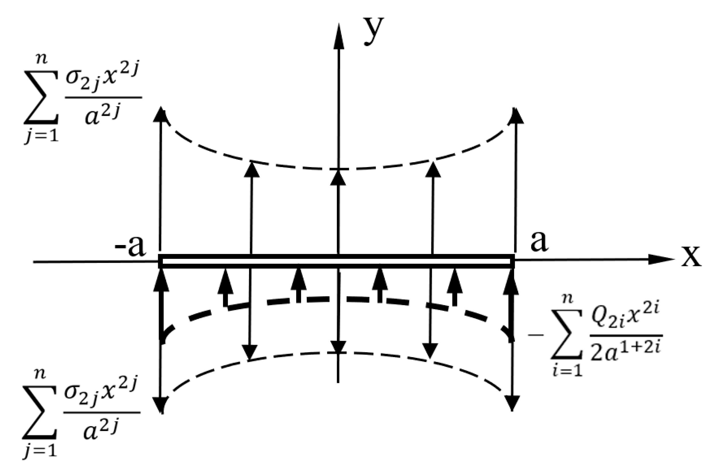
2. Problem Statement

A single crack embedded in an orthotropic solid is shown in Figure 1. And 2i order polynomial function thermal flux and 2j order polynomial function mechanical loading are considered.

The constitute equations are given based on the state of plane stress:

$${\sigma }_{xx}=c_{11}\frac{\partial u}{\partial x}+c_{12}\frac{\partial v}{\partial y}-{\beta }_1\theta ,$$

(2)

$${\sigma }_{yy}=c_{12}\frac{\partial u}{\partial x}+c_{22}\frac{\partial v}{\partial y}-{\beta }_2\theta ,$$

(3)

$${\sigma }_{xy}=c_{66}[\frac{\partial u}{\partial y}+\frac{\partial v}{\partial x}],$$

(4)

where

$$c_{11}=\frac{E_{xx}}{1-v_{xy}{v}_{yx}}, c_{22}=\frac{E_{yy}}{1-v_{xy}{v}_{yx}},$$

(5)

$$c_{12}=\frac{E_{xx}{v}_{yx}}{1-v_{xy}{v}_{yx}}=\frac{E_{yy}{v}_{xy}}{1-v_{xy}{v}_{yx}},$$

(6)

$$\left[\begin{array}{c}{\beta }_1\\ {\beta }_2\end{array}\right]=\left[\begin{array}{cc}{c}_{11}& c_{12}\\ c_{12}& c_{22}\end{array}\right]\left[\begin{array}{c}{\alpha }_{xx}\\ {\alpha }_{yy}\end{array}\right],$$

(7)

where ${\sigma }_{yy}$ and ${\sigma }_{xy}$ represent the components of stress, $E_{xx}$ and $E_{yy}$ denote the Young’s moduli, $\theta$ is the temperature, $v_{xx}$ and $v_{yy}$ indicate the Poisson’s ratios, $u$ and $v$ represent the components of elastic displacement, $c_{66}=G_{xy}$ represent the shear modulus, and ${\alpha }_{xx}$ and ${\alpha }_{yy}$ are the coefficients of linear expansion. Utilizing the following equations:

$$\frac{\partial {\sigma }_{xx}}{\partial x}+\frac{\partial {\sigma }_{xy}}{\partial y}=0,\frac{\partial {\sigma }_{xy}}{\partial x}+\frac{\partial {\sigma }_{yy}}{\partial y}=0$$

(8)

one obtains

$$c_{11}\frac{{\partial }^{2}u}{\partial x^2}+c_{66}\frac{{\partial }^{2}u}{\partial y^2}+(c_{12}+c_{66})\frac{{\partial }^{2}v}{\partial x\partial y}={\beta }_1\frac{\partial T}{\partial x}$$

(9)

$$c_{66}\frac{{\partial }^{2}v}{\partial x^2}+c_{22}\frac{{\partial }^{2}v}{\partial y^2}+(c_{12}+c_{66})\frac{{\partial }^{2}u}{\partial x\partial y}={\beta }_2\frac{\partial T}{\partial y}$$

(10)

Based on the Fourier heat conduction, it can be obtained as follows:

$$Q_x=-{\lambda }_x\frac{\partial T}{\partial x},Q_y=-{\lambda }_y\frac{\partial T}{\partial y}$$

(11)

where $Q_x$, $Q_y$ denote the components of the heat flux, and ${\lambda }_x$ and ${\lambda }_y$ denote the coefficient of heat conduction. Furthermore, in accordance with equilibrium equation, one leads to

$$\frac{\partial Q_x}{\partial x}+\frac{\partial Q_y}{\partial y}=0$$

(12)

and assuming thermal equilibrium equation, one obtains

$${\lambda }^2\frac{{\partial }^{2}T}{\partial x^2}+\frac{{\partial }^{2}T}{\partial y^2}=0$$

(13)

where

$$\lambda =\sqrt{\frac{{\lambda }_x}{{\lambda }_y}}$$

(14)

In this paper, we take advantage of the crack-face boundary conditions as follows:

$$Q_y^I(x,0)-Q_y^{II}(x,0)=-(Q_{0i}-Q_{\mathrm{c}i}){\displaystyle \sum _{i=0}^n\frac{x^{2i}}{2a^{2i+1}}}\hspace{1em} -a<x<a$$

(15a)

$${\sigma }_{{}_{yy}}^{II}(x,0)={\sigma }_{{}_{yy}}^I(x,0)={\displaystyle \sum _{j=0}^n\frac{{\sigma }_{2j}}{a^{2j}}{x}^{2j}}\hspace{1em} -a<x<a$$

(15b)

The superscripts $I$ and $II$ represent the physical quantities of $y>0$ and $y<0$ region, respectively. $Q_i$ and ${\sigma }_{2j}$ denote the prescribed constants. With the symmetry of the thermomechanical loadings in account, we simply consider half of the thermo-elastic field (i.e., $x>0$ and $-\infty <y<+\infty$) under the thermomechanical loadings $-{\displaystyle \sum _{i=0}^n{Q}_{0i}{x}^{2i}/2a^{2i+1}}$ and ${\displaystyle \sum _{j=0}^n{\sigma }_{2j}{x}^{2j}/a^{2j}}$. The following boundary conditions of the crack-surface are depicted as

$${\sigma }_{xy}^I(x,0)={\sigma }_{xy}^{II}(x,0)=0\hspace{1em} \hspace{1em} 0<x<a$$

(16)

$$Q_y^{II}(x,0)-Q_y^I(x,0)=-(Q_{0i}-Q_{ci}){\displaystyle \sum _{i=0}^n{x}^{2i}/2a^{2i+1}}\hspace{1em} \hspace{1em} 0<x<a$$

(17a)

$${\sigma }_{yy}^{II}(x,0)={\sigma }_{yy}^I(x,0)={\displaystyle \sum _{j=0}^n\frac{{\sigma }_{2j}^{}}{a^{2j}}{x}^{2j}}\hspace{1em} \hspace{1em} 0<x<a$$

(17b)

From Equations (17a) to (17b), the thermal flux and the mechanical loading consist of several parts. Firstly, the solutions under the thermal flux $-Q_{0i}{x}^{2i}/2a^{2i+1}$ and mechanical loading ${\sigma }_{2j}{x}^{{}_{2j}}/a^{{}_{2j}}$ will be given. Secondly, utilizing principle of superposition, such expressions as temperature change, elastic displacement on the crack and stresses under thermal flux $-{\displaystyle \sum _{i=0}^n{Q}_{0i}{x}^{2i}/2a^{2i+1}}$, and mechanical loading ${\displaystyle \sum _{j=0}^n{\sigma }_{2j}{x}^{2j}}/a^{2j}$, will be obtained. The thermo-elastic boundary conditions across the crack-surface subjected to the thermal flux $-Q_{0i}{x}^{2i}/2a^{2i+1}$ and mechanical loading ${\sigma }_{2j}/a^{2j}$ are as follows.

$${\sigma }_{xy}^I(x,0)={\sigma }_{xy}^{II}(x,0)=0\hspace{1em} \hspace{1em} \hspace{1em} 0<x<a$$

(18)

$$Q_y^I(x,0)-Q_y^{II}(x,0)=-\frac{(Q_{0i}-Q_{ci})x^{2i}}{2a^{2i+1}},{\sigma }_{yy}^{II}(x,0)={\sigma }_{yy}^I(x,0)=\frac{{\sigma }_{2j}}{a^{2j}}{x}^{2j}\hspace{1em} 0<x<a$$

(19)

where

$$Q_{ci}=-h_c(T_{}^I(x,0)-T_{}^{II}(x,0))+\epsilon Q_{i0}$$

(20)

Moreover, such factors as stresses, elastic displacements, and temperature and heat flux across the crack-free region of the horizontal x-axis comply with the following conditions.

$${\sigma }_{{}_{xy}}^I(x,0)={\sigma }_{{}_{xy}}^{II}(x,0), {\sigma }_{yy}^I(x,0)={\sigma }_{yy}^{II}(x,0) x>a or x<-a$$

(21)

$$u_{}^I(x,0)=-u_{}^{II}(x,0), v_{}^I(x,0)= -v^{II}(x,0)\hspace{1em} x>a or x<-a$$

(22)

$$T_{}^I(x,0)=T_{}^{II}(x,0),\hspace{1em} Q_{{}_y}^I(x,0)=Q_{{}_y}^{II}(x,0)\hspace{1em} x>a or x<-a$$

(23)

3. Solution Procedure

3.1. Temperature Field

The temperature field can be solved out first now that Equation (13) is irrelevant to the elastic strain. With application of FTT, one can depict the solution of Equation (13) as follows:

$$T_{}^{I,II}(x,y)={\displaystyle {\int }_0^{+\infty }{g}_{}^{\pm }(\xi )e^{-\xi {\delta }^{\pm }\lambda y}\cos }(\xi x)d\xi$$

(24)

$g_{}^{\pm }(\xi )$ are unknown and will be solved. ${\delta }^{+}=1$ and ${\delta }^{-}=-1$ denote $y>0$ and $y<0$, respectively. From (11), one gets

$$Q_x^{I,II}(x,y)={\lambda }_x{\displaystyle {\int }_{ 0}^{ \infty }\xi g^{\pm }(\xi )e^{-\xi {\delta }^{\pm }\lambda y}\sin (\xi x)d\xi }$$

(25)

$$Q_y^{I,II}(x,y)={\lambda }_y\lambda {\displaystyle {\int }_{ 0}^{ \infty }{\delta }^{\pm }\xi g^{\pm }(\xi )e^{-\xi {\delta }^{\pm }\lambda y}\cos (\xi x)d\xi }$$

(26)

Applying the second relation in Equation (23), one gets

$$g_{}^{+}(\xi )=-g_{}^{-}(\xi )$$

(27)

Utilizing the first relation in Equations (23) and (19), one attains

$${\displaystyle {\int }_0^{+\infty }{g}^{+}}(\xi )\cos (\xi x)d\xi =0\hspace{1em} x>a$$

(28)

$${\displaystyle {\int }_0^{+\infty }{g}^{+}}(\xi )\cos (\xi x)d\xi =-\frac{(Q_{ci}-Q_{0i})x^{2i}}{4a^{2i+1}\lambda {\lambda }_y} 0<x<a$$

(29)

For the solvation of Equations (28) and (29), the auxiliary function ${\gamma }_{2i}(x)$ is defined as

$$\gamma (x)=\frac{\partial [T^I(x,0)-T^{II}(x,0)]}{\partial x}$$

(30)

Applying inverse Fourier transform leads to

$$g^{+}(\xi )\xi =-\frac{1}{\pi }{\displaystyle {\int }_0^a\gamma }(s)\sin (\xi s)ds$$

(31)

Substituting Equation (31) into (29), one gets

$$\frac{2}{\pi }{\displaystyle {\int }_0^a\gamma }(s)ds{\displaystyle {\int }_0^{+\infty }\sin }(\xi s)\cos (\xi x)d\xi =\frac{(Q_{0i}-Q_{ci})x^{2i}}{2a^{2i+1}\lambda {\lambda }_y}$$

(32)

from the known result [29].

$${\displaystyle {\int }_0^{+\infty }\cos (\xi x)\sin }(\xi s)d\xi =\frac{1}{2}(\frac{1}{s-x}+\frac{1}{s+x})$$

(33)

Equation (32) can be expressed as follows:

$$\frac{1}{\pi }{\displaystyle {\int }_{-a}^a\gamma }(s)\frac{1}{s-x}ds=\frac{(Q_{0i}-Q_{ci})x^{2i}}{2a^{2i+1}\lambda {\lambda }_y}$$

(34)

Equation (34) features a singular integral equation including the Cauchy kernel [28], and the solution can be unraveled as

$$\gamma (x)=\frac{1}{\pi \sqrt{a^2-x^2}}{\displaystyle {\int }_{-a}^a\frac{\sqrt{a^2-s^2}}{x-s}}\frac{(Q_{0i}-Q_{ci})s^{2i}}{2a^{2i+1}\lambda {\lambda }_y}ds+\frac{C_{2i}}{\sqrt{a^2-x^2}}$$

(35)

Considering the following condition:

$${\displaystyle {\int }_{-a}^a\gamma (s)ds=0}$$

(36)

After some computations, one has $C_{2i}=0$, and Equation (35) can be given as

$$\gamma (x)=\frac{(Q_{0i}-Q_{ci})x}{2a\lambda {\lambda }_y\pi \sqrt{a^2-x^2}} i=0$$

(37a)

$$\gamma (x)=-{\displaystyle \sum _{j=0}^{2i-1}\frac{(Q_{0i}-Q_{ci})x^j}{2a^{2i+1}\lambda {\lambda }_y\pi \sqrt{a^2-x^2}}}{I}_j+\frac{(Q_{0i}-Q_{ci})}{2a^{2i+1}\lambda {\lambda }_y\sqrt{a^2-x^2}}{x}^{2i+1} i\ge 1$$

(37b)

where

$$I_l=-{\displaystyle {\int }_{-a}^a\sqrt{(a^2-s^2)}}{s}^{2i-l-1}ds\left(1\le l\le 2i-1\right).$$

(38)

In addition, with application of Equations (30), (37a) and (37b), the temperature change on the crack is given as

$$T_{}^I(x,0)-T_{}^{II}(x,0)=-\frac{(Q_{00}-Q_{\mathrm{c}0})}{a\lambda {\lambda }_y}\sqrt{a^2-x^2} i=0$$

(39a)

$$T^I(x,0)-T_{}^{II}(x,0)=-{\displaystyle \sum _{l=0}^{2i-1}\frac{(Q_{0i}-Q_{ci})I_l}{2a^{2i+1}\lambda {\lambda }_y\pi \sqrt{a^2-x^2}}}{\displaystyle {\int }_{-a}^x\frac{s^l}{\sqrt{a^2-s^2}}}ds+\frac{(Q_{0i}-Q_{ci})}{2a^{2i+1}\lambda {\lambda }_y}{\displaystyle {\int }_{-a}^x\frac{s^{2i+1}}{\sqrt{a^2-s^2}}}ds i\ge 1$$

(39b)

where

$$\begin{array}{l}E(x,l)={\displaystyle {\int }_{-a}^x\frac{s^l}{\sqrt{a^2-s^2}}}ds l=2k<2i-1\\ =\left[\frac{1}{2^l}\left(\begin{array}{c}l\\ l/2\end{array}\right)\arcsin (x)+\frac{{(-1)}^{l/2}}{2^{l-1}}{\displaystyle \sum _{m=0}^{l/2-1}{(-1)}^m}\left(\begin{array}{c}l\\ m\end{array}\right)\frac{\sin [l-2m)(\arcsin (x/a))]}{l-2m}\right]\\ -\left[-\frac{\pi }{2^{l+1}}\left(\begin{array}{c}l\\ l/2\end{array}\right)+\frac{{(-1)}^{l/2}}{2^l}{\displaystyle \sum _{m=0}^{l/2-1}{(-1)}^m}\left(\begin{array}{c}l\\ m\end{array}\right)\frac{\sin [-(l-2m)\pi /2]}{l-2m}\right]\end{array}$$

(40a)

$$\begin{array}{l}E(x,l)={\displaystyle {\int }_{-a}^x\frac{s^l}{\sqrt{a^2-s^2}}}ds l=2k+1\le 2i-1\\ =\frac{{(-1)}^{(l+1)/2}}{2^{l-1}}{\displaystyle \sum _{m=0}^{(l-1)/2}{(-1)}^m}\left(\begin{array}{c}l\\ m\end{array}\right)\frac{\cos [(l-2m)(\arcsin (x/a))]}{l-2m}\\ -\frac{{(-1)}^{(l+1)/2}}{2^{l-1}}{\displaystyle \sum _{m=0}^{(l-1)/2}{(-1)}^m}\left(\begin{array}{c}l\\ m\end{array}\right)\frac{\cos [(l-2m)\pi /2]}{l-2m}\end{array}$$

(40b)

$$\begin{array}{l}F(x,i)={\displaystyle {\int }_{-a}^x\frac{s^{2i+1}}{\sqrt{a^2-s^2}}}ds \\ =\frac{{(-1)}^{i+1}}{2^{2i}}{\displaystyle \sum _{m=0}^i{(-1)}^m}\left(\begin{array}{c}2i+1\\ m\end{array}\right)\frac{\cos [(2i+1-2m)(\arcsin (x/a))]}{2i+1-2m}\\ -\frac{{(-1)}^{i+1}}{2^{2i}}{\displaystyle \sum _{m=0}^i{(-1)}^m}\left(\begin{array}{c}2i+1\\ m\end{array}\right)\frac{\cos [\pi (2i+1-2m)/2]}{2i+1-2m}\end{array}$$

(40c)

3.2. Elastic Field

In order to solve Equations (9) and (10), $u_{{}_{}}^{I,II}(x,y)$ and $v_{{}_{}}^{I,II}(x,y)$ are written as [19]

$$u_{{}_{}}^{I,II}(x,y)=u_1^{I,II}(x,y)+u_2^{I,II}(x,y),v_{{}_{}}^{I,II}(x,y)=v_{{}_1}^{I,II}(x,y)+v_1^{I,II}(x,y)$$

(41)

$u_{{}_1}^{I,II}(x,y)$ and $v_{{}_1}^{I,II}(x,y)$ respond to the general solutions under $T_{}^{I,II}(x,y)=0$. $u_{{}_2}^{I,II}(x,y)$ and $v_2^{I,II}(x,y)$ are the peculiar solutions subjected to thermal flux loading. With application of FTT, $u_{{}_1}^{I,II}(x,y)$ and $v_{{}_1}^{I,II}(x,y)$ can be written as

$$u_{{}_1}^{I,II}(x,y)={\displaystyle \sum _{j=1}^2{\displaystyle {\int }_0^{+\infty }{g}_{{}_j}^{\pm }}}(\xi )e^{-\xi {\delta }^{\pm }{\gamma }_{j}y}\sin (\xi x)d\xi$$

(42)

$$v_1^{I,II}(x,y)={\displaystyle \sum _{j=1}^2{\displaystyle {\int }_0^{+\infty }{\eta }_j{\delta }^{\pm }{g}_j^{\pm }}}(\xi )e^{-\xi {\delta }^{\pm }{\gamma }_{j}y}\cos (\xi x)d\xi$$

(43)

$g_{{}_j}^{\pm }(\xi )$ have not been solved. ${\gamma }_j(j=1,2)$($Re{\gamma }_j>0$) are the roots of character equation as follows:

$$c_{22}{c}_{66}{\gamma }_{}^4+(c_{12}^2+2c_{12}{c}_{66}-c_{12}{c}_{22}){\gamma }_{}^2+c_{11}{c}_{66}=0$$

(44)

where

$${\eta }_j=\frac{c_{11}-c_{66}{\gamma }_j^2}{(c_{12}+c_{66}){\gamma }_j}$$

(45)

Furthermore, $u_2^{I,II}(x,y)$ and $v_2^{I,II}(x,y)$ are chosen as

$$u_2^{I,II}(x,y)={\displaystyle \sum _{j=1}^2{\displaystyle {\int }_0^{+\infty }{g}_{}^{*\pm }(\xi )}{e}^{-\delta \pm \xi \lambda y}\sin (\xi x)d\xi }$$

(46)

$$v_2^{I,II}(x,y)={\displaystyle \sum _{j=1}^2{\displaystyle {\int }_0^{+\infty }{\delta }^{\pm }{L}_{}^{*\pm }(\xi )}{e}^{-\delta \pm \xi \lambda y}\cos (\xi x)d\xi }$$

(47)

Substituting Equations (46) and (47) into Equations (9) and (10), one has

$$\left[\begin{array}{c}{g}_{}^{*\pm }(\xi )\\ L_{}^{*\pm }(\xi )\end{array}\right]=\left[\begin{array}{c}{K}_1\\ K_2\end{array}\right]\frac{g_{}^{\pm }(\xi )}{\xi }$$

(48)

where

$$\left[\begin{array}{c}{K}_1\\ K_2\end{array}\right]={\left[\begin{array}{cc}{c}_{11}-c_{66}{\lambda }^2& -(c_{12}+c_{66})\lambda \\ (c_{12}+c_{66})\lambda & c_{66}-c_{22}{\lambda }^2\end{array}\right]}^{-1}\left[\begin{array}{c}{\beta }_1\\ {\beta }_2\lambda \end{array}\right]$$

(49)

Based on Equations (2)–(4), (42), (43), (46) and (47), the components of stress are rewritten as

$$\begin{array}{l}{\sigma }_{xx}^{I,II}(x,0)={\displaystyle \sum _{j=1}^2{\displaystyle {\int }_0^{+\infty }(c_{11}-c_{12}{\gamma }_j{\eta }_j)\xi g_j^{\pm }}}(\xi )\cos (\xi x)d\xi \\ \begin{array}{ccc}& & \end{array}+(c_{11}{M}_1-c_{12}\lambda M_2-{\beta }_1){\displaystyle {\int }_0^{+\infty }{g}^{\pm }(\xi )}\cos (\xi x)d\xi \end{array}$$

(50)

$$\begin{array}{l}{\sigma }_{yy}^{I,II}(x,0)={\displaystyle \sum _{j=1}^2{\displaystyle {\int }_0^{+\infty }(c_{12}-c_{22}{\gamma }_j{\eta }_j)\xi g_j^{\pm }}}(\xi )\cos (\xi x)d\xi \\ \begin{array}{ccc}& & \end{array}+(c_{12}{M}_1-c_{22}\lambda M_2-{\beta }_2){\displaystyle {\int }_0^{+\infty }{g}_{}^{{}^{\pm }}(\xi )\cos }(\xi x)d\xi \end{array}$$

(51)

$$\begin{array}{l}{\sigma }_{xy}^{I,II}(x,0)=-c_{66}[{\displaystyle \sum _{j=1}^2{\displaystyle {\int }_0^{+\infty }{\delta }^{\pm }({\gamma }_j+{\eta }_j)\xi g_j^{\pm }}}(\xi )\sin (\xi x)d\xi \\ \begin{array}{ccc}& & +{\displaystyle {\int }_0^{+\infty }{\delta }^{\pm }(M_1\lambda +M_2)g^{\pm }(\xi )}\sin (\xi x)d\xi ]\end{array}\end{array}$$

(52)

To solve the problem, it is divided into two parts. One part is what is resulted from mechanical loading ${\sigma }_{2j}{x}^{2j}/a^{2j}$. The other part is what is induced by thermal flux $-Q_{0i}{x}^{2i}/2a^{2i+1}$. Firstly, the mechanical loading is considered and the dual integral equations are written.

$${\sigma }_{xy}^I(x,0)={\sigma }_{xy}^{II}(x,0)=0 x>0$$

(53)

$$v^I(x,0)=-v_{}^{II}(x,0)=0 x>a$$

(54)

Utilizing Equations (53) and (54), one obtains

$$g_j^{+}(\xi )=g_j^{-}(\xi ), g_2^{+}(\xi )=-\frac{{\gamma }_1+{\eta }_1}{{\gamma }_2+{\eta }_2}{g}_1^{-}(\xi )$$

(55)

Applying the second relation in Equations (19) and (54), one arrives at

$${\displaystyle {\int }_0^{+\infty }\xi g_1^{+}(\xi )}\cos (\xi x)d\xi =0 x>a$$

(56)

$${\displaystyle {\int }_0^{+\infty }\xi g_1^{+}(\xi )}\cos (\xi x)d\xi =\frac{{\sigma }_{2j}{x}^{2i}}{{\omega }_1{a}^{2i}} 0<x<a$$

(57)

where

$${\omega }_1=(c_{12}-c_{22}{\gamma }_1{\eta }_1)-\frac{{\gamma }_1+{\eta }_1}{{\gamma }_2+{\eta }_2}(c_{12}-c_{22}{\gamma }_2{\eta }_2)$$

(58)

The auxiliary function $\varphi (x)$ is chosen to solve Equations (56) and (57),

$$\varphi (x)=\frac{\partial v^I(x,0)}{\partial x}$$

(59)

With knowledge of inverse Fourier transform (IFT), one has

$$g_1^{+}(\xi )\xi =-\frac{2({\gamma }_2+{\eta }_2)}{({\eta }_1{\gamma }_2-{\eta }_2{\gamma }_1)\pi }{\displaystyle {\int }_0^a\varphi }(s)\sin (\xi s)ds$$

(60)

According to the known result of Equation (33), inserting Equation (60) into (57), we have

$$\frac{1}{\pi }{\displaystyle {\int }_{-a}^a\frac{\varphi (s)}{s-x}}ds=\frac{{\sigma }_{2j}({\eta }_1{\gamma }_2-{\eta }_2{\gamma }_1)}{{\omega }_1({\gamma }_2+{\eta }_2)a^{2j}}{x}^{2j}$$

(61)

Based on the singular integral theory including the Cauchy kernel, the following solution is given:

$$\varphi (x)=\frac{1}{\pi \sqrt{a^2-x^2}}{\displaystyle {\int }_{-a}^a\frac{\sqrt{a^2-s^2}}{x-s}}\frac{{\sigma }_{2j}({\eta }_1{\gamma }_2-{\eta }_2{\gamma }_1)}{{\omega }_1({\gamma }_2+{\eta }_2)a^{2j}}{s}^{2j}ds+\frac{D_{2j}}{\sqrt{a^2-x^2}}$$

(62)

After some computations, $D_{2j}=0$. With application of Equations (59) and (62), one obtains the elastic displacement as

$$v^I(x,0)={\displaystyle {\int }_{-a}^x{\varphi }_{}(s)}ds=\frac{{\sigma }_0({\eta }_1{\gamma }_2-{\eta }_2{\gamma }_1)\sqrt{a^2-x^2}}{{\omega }_1({\gamma }_2+{\eta }_2)} j=0$$

(63a)

$$v_{}^I(x,0)={\displaystyle {\int }_{-a}^x\varphi (s)}ds=-{\displaystyle \sum _{l=0}^{2j-1}\frac{{\sigma }_{2j}({\eta }_1{\gamma }_2-{\eta }_2{\gamma }_1)I_l}{{\omega }_1({\gamma }_2+{\eta }_2)\pi a^{2j}\sqrt{a^2-x^2}}}{\displaystyle {\int }_{-a}^x\frac{s^l}{\sqrt{a^2-s^2}}}ds+\frac{{\sigma }_{2j}({\eta }_1{\gamma }_2-{\eta }_2{\gamma }_1)}{{\omega }_1({\gamma }_2+{\eta }_2)a^{2j}}{\displaystyle {\int }_{-a}^x\frac{s^{2j+1}}{\sqrt{a^2-s^2}}}ds j\ge 1$$

(63b)

Furthermore, one can obtain the stress fields as follows:

$${\sigma }_{{}^{yy}}^{I,II}(x,0)=-\left(1-\frac{x}{\sqrt{x^2-a^2}}\right){\sigma }_0 j=0$$

(64)

$${\sigma }_{{}_{yy}}^{I,II}(x,0)=-{\displaystyle {\int }_{-a}^a\frac{{\sigma }_{2j}{\displaystyle \sum _{l=0}^{2j-1}{s}^l}{I}_l}{a^{2j}\sqrt{a^2-s^2}(s-x)}ds}+{\displaystyle {\int }_{-a}^a\frac{{\sigma }_{2j}{s}^{2j+1}}{a^{2j}\sqrt{a^2-s^2}(s-x)}ds} j\ge 1$$

(65)

Then, the explicit solution of elastic field under 2i order polynomial function thermal flux will be obtained. With the application of heat flux, it fits in the following condition.

$${\sigma }_{yy}^I(x,0)={\sigma }_{yy}^{II}(x,0)=0 0<x<a$$

(66)

With application of Equations (51) and (66), one arrives at

$$g_j^{+}(\xi )=-g_j^{-}(\xi )$$

(67)

$${\displaystyle \sum _{j=1}^2(c_{12}-c_{22}{\gamma }_j{\eta }_j)}{g}_j^{+}(\xi )=(c_{22}\lambda M_2+{\beta }_2-c_{12}{M}_1)\frac{g_{}^{+}(\xi )}{\xi }$$

(68)

With application of Equation (16), one can depict the first relation in Equation (22), and the dual integral equations are:

$${\displaystyle {\int }_0^{+\infty }\left[{\displaystyle \sum _{j=1}^2{g}_j^{+}(\xi )}\sin (\xi x)+\frac{M_1{g}_{}^{+}(\xi )}{\xi }\sin (\xi x)\right]} d\xi =0 x>a$$

(69)

$${\displaystyle {\int }_0^{+\infty }{\displaystyle \sum _{j=1}^2({\gamma }_j+{\eta }_j)\xi g_j^{+}(\xi )}\sin (\xi x)}d\xi +{\displaystyle {\int }_0^{+\infty }(M_1}\lambda +M_2)g^{+}(\xi )\sin (\xi x)d\xi =0 0<x<a$$

(70)

To achieve the solvation of Equations (69) and (70), the auxiliary function $\chi (x)$ can be defined as

$${\chi }_{{}_{}}(x)=\frac{\partial u_{}^I(x,0)}{\partial x}$$

(71)

Applying Equation (69) and inverse Fourier transform leads to

$${\displaystyle \sum _{j=1}^2{g}_j^{+}(\xi )}\xi +M_1{g}_{}^{+}(\xi )=\frac{2}{\pi }{\displaystyle {\int }_0^a{\chi }_{}(s)} \cos (\xi s)ds$$

(72)

Utilizing Equations (68) and (72), one obtains

$$g_1^{+}(\xi )\xi =\frac{c_{22}\lambda M_2+{\beta }_2-c_{22}{\gamma }_2{\eta }_2{M}_1}{c_{22}({\gamma }_2{\eta }_2-{\gamma }_1{\eta }_1)}{g}_{}^{+}(\xi )+\frac{c_{22}{\gamma }_2{\eta }_2-c_{12}}{c_{22}({\gamma }_2{\eta }_2-{\gamma }_1{\eta }_1)}\frac{2}{\pi }{\displaystyle {\int }_0^a{\chi }_{}(s)}\cos (\xi s)ds$$

(73)

$$g_2^{+}(\xi )\xi =\frac{c_{22}{\gamma }_1{\eta }_1{M}_1-c_{22}\lambda M_2-{\beta }_2}{c_{22}({\gamma }_2{\eta }_2-{\gamma }_1{\eta }_1)}{g}_{}^{+}(\xi )+\frac{c_{12}-c_{22}{\gamma }_1{\eta }_1}{c_{22}({\gamma }_2{\eta }_2-{\gamma }_1{\eta }_1)}\frac{2}{\pi }{\displaystyle {\int }_0^a\chi (s)} \cos (\xi s)ds$$

(74)

With application of Equations (70), (73) and (74), one obtains

$$2{\displaystyle {\int }_0^a\chi (s)}ds{\displaystyle {\int }_0^{+\infty }\sin (\xi x)\cos (\xi s)}d\xi =\pi {\omega }_2{\displaystyle {\int }_0^{+\infty }{g}_{}^{+}(\xi )}\sin (\xi x)d\xi 0<x<a$$

(75)

where

$${\omega }_2=\frac{H_1}{H_2}$$

(76)

With

$$\begin{array}{l}{H}_1=({\gamma }_1+{\eta }_1)(c_{22}{\gamma }_2{\eta }_2{M}_1-c_{22}\lambda M_2-{\beta }_2)+({\gamma }_2+{\eta }_2)\\ (c_{22}\lambda M_2+{\beta }_2-c_{22}{\gamma }_1{\eta }_1{M}_1)+c_{22}(M_1\lambda +M_2)({\gamma }_1{\eta }_1-{\gamma }_2{\eta }_2)\end{array}$$

(77)

$$H_2=({\gamma }_1+{\eta }_1)(c_{22}{\gamma }_2{\eta }_2-c_{12})+({\gamma }_2+{\eta }_2)(c_{12}-c_{22}{\gamma }_1{\eta }_1)$$

(78)

With the knowledge of Equation (35), Equation (75) can be rewritten as

$$\frac{1}{\pi }{\displaystyle {\int }_{-a}^a\frac{\chi (s)}{x-s}}ds={\omega }_2{\displaystyle {\int }_0^{+\infty }{g}_{}^{+}(\xi )}\sin (\xi x)d\xi$$

(79)

The use of Equation (24) and the inverse Fourier transform leads to

$$\begin{array}{l}{\displaystyle {\int }_0^{+\infty }{g}_{}^{+}(\xi )}\sin (\xi x)d\xi =-\frac{2}{\pi }{\displaystyle {\int }_0^{+\infty }\chi (s)ds{\displaystyle {\int }_0^{+\infty }\frac{\sin (\xi x)\sin (\xi s)}{\xi }}}d\xi \\ =-\frac{1}{\pi }{\displaystyle {\int }_0^{+\infty }\chi (s)\ln \left|\frac{x+s}{x-s}\right|ds}\end{array}$$

(80)

from the known result [29].

$${\displaystyle {\int }_0^{+\infty }\frac{1}{\xi }}\sin (\xi x)\sin (\xi s)d\xi =\frac{1}{2}\ln \left|\frac{x+s}{x-s}\right|$$

(81)

According to the singular integral theory with the Cauchy kernel, Equation (79) is obtained:

$$\chi (x)=\frac{{\omega }_2}{\pi \sqrt{a^2-x^2}}{\displaystyle {\int }_{-a}^a\frac{\sqrt{a^2-t^2}}{x-t}dt}{\displaystyle {\int }_0^{+\infty }\gamma (s)\ln \left|\frac{t+s}{t-s}\right|ds}$$

(82)

With application of Equation (71), one obtains

$$u_{}^I(x,0)={\displaystyle {\int }_{-a}^x\chi }(s)ds$$

(83)

From Equations (52), (73), (74) and (80), one can obtain the shearing stresses as follows:

$${\sigma }_{xy}^{I,II}(x,0)=\frac{c_{66}}{\pi c_{22}({\gamma }_2{\eta }_2-{\gamma }_1{\eta }_1)}{\displaystyle {\int }_{-a}^a\left[\frac{H_2\chi (s)}{s-x}-H_1\gamma (s)\ln \left|\frac{x+s}{x-s}\right|\right]}ds$$

(84)

The shearing stresses are given, which is distinct from the achieved results for cracked solid under combined constant thermal flux and constant mechanical loading [19]. Taking the advantage of principle of superposition, such expressions as temperature change, elastic displacement on the crack, and stresses under combined 2i order polynomial function thermal flux and 2j order polynomial function mechanical loading can be given.

3.3. Crack-Tip Field

The behavior of the stress intensity factors (SIF) is of much importance, and the corresponding SIF are given as

$$K_I=\underset{x\to a^{+}}{\lim }\sqrt{2\pi (x-a)}{\sigma }_{yy}^I(x,0)$$

(85)

$$K_{II}=\underset{x\to a^{+}}{\lim }\sqrt{2\pi (x-a)}{\sigma }_{xy}^I(x,0)$$

(86)

Next, we define the corresponding intensity factors to characterize opening crack displacement.

$$K_v^{COD}=\underset{x\to a^{+}}{\lim }\sqrt{\frac{\pi }{2(a-x)}}{v}^I(x,0)$$

(87)

$$K_u^{COD}=\underset{x\to a^{+}}{\lim }\sqrt{\frac{\pi }{2(a-x)}}{u}^I(x,0)$$

(88)

The energy release rate has an important effect on the analysis of crack growth, and the energy release rate is defined as

$$G_{}=\underset{\delta \to 0}{\lim }\frac{1}{\delta }{\displaystyle {\int }_0^{\delta }{\sigma }_{xy}^I(x+a,0)u_{}^I(a-x,0)+{\sigma }_{yy}^I(x+a,0)v_{}^I(a-x,0)dx}$$

(89)

The energy density dW/dV featuring positive definiteness is of fundamental significance to the formulation of mechanics theories and physics of solids. As for non-iso-thermal problem, the strain energy which is reserved in a unit volume of the orthotropic solid is written [2,30].

$$\frac{dW}{dV}=\frac{S}{r}=\frac{1}{2}{\sigma }_{ij}{\epsilon }_{ij}-\frac{1}{2}{\alpha }_{kk}\theta {\sigma }_{kk}$$

(90)

where S indicates the strain energy density factor, along with r representing the reach to the crack tip. The application of concepts above entails an understanding of the energy density function. For the orthotropic solid, Equation (90) can also be illustrated as

$$\frac{dW}{dV}=\frac{S}{r}=\frac{1}{2}\left(\frac{c_{22}{\sigma }_{xx}^2{}^{}+c_{11}{\sigma }_{yy}^2{}^{}-2c_{12}{\sigma }_{xx}^{}{\sigma }_{{}_{yy}}^{}}{2c_{11}{c}_{22}-c_{12}^2}+\frac{{\sigma }_{xy}^2{}^{}}{c_{66}}\right)$$

(91)

Furthermore, the strain energy density factor on the crack line have an effect on the analysis of crack growth. That is, we have

$$S_0=\frac{1}{4\pi }\left(\frac{c_{22}{w}^2+c_{11}-2c_{12}w}{c_{11}{c}_{22}-c_{{}_{12}}^2}{K}_{{}_I}^2+\frac{1}{c_{66}}{K}_{II}^2\right)$$

(92)

where

$$w=\frac{1}{w_1}{\displaystyle \sum _{j=1}^2{(-1)}^j}\frac{{\gamma }_1+{\eta }_1}{{\gamma }_j+{\eta }_j}(c_{11}-c_{12}{\gamma }_j{\eta }_j)$$

(93)

3.4. Explicit Expressions for the Particular Case of Combined the Constant Thermo-Mechanical Loading

According to the above results, the thermoelastic field in the full plane under combined the constant thermal flux $-(Q_{00}-Q_{c0})/2a$ and the constant mechanical loading ${\sigma }_0$ can be given inexplicit form.

$${\sigma }_{{}_{yy}}^{I,II}(x,0)=-\left(1-\frac{x}{\sqrt{x^2-a^2}}\right){\sigma }_0$$

(94)

$${\sigma }_{{}_{xy}}^{I,II}(x,0)=-\frac{c_{66}{\omega }_2(Q_{00}-Q_{c0})a}{2c_{22}\lambda {\lambda }_y({\gamma }_2{\eta }_2-{\gamma }_1{\eta }_1)\sqrt{x^2-a^2}}$$

(95)

$$u^I(x,0)=-\frac{(Q_{00}-Q_{c0}){\omega }_{2}x\sqrt{a^2-x^2}}{4\lambda {\lambda }_y}$$

(96)

$$v_{}^I(x,0)=\frac{{\sigma }_0({\eta }_1{\gamma }_2-{\eta }_2{\gamma }_1)}{{\omega }_1({\gamma }_2+{\eta }_2)}\sqrt{a^2-x^2}$$

(97)

With application of Equations (85)–(88) and (94)–(97), one has

$$K_I={\sigma }_0\sqrt{\pi a}$$

(98)

$$K_{II}=\frac{c_{66}{\omega }_2(Q_{c0}-Q_{00})\sqrt{\pi a}}{2\lambda {\lambda }_y{c}_{22}({\rho }_2{\eta }_2-{\rho }_1{\eta }_1)}$$

(99)

$$K_u^{COD}=\frac{(Q_{c0}-Q_{00}){\omega }_2\sqrt{\pi a}}{4\lambda {\lambda }_y}$$

(100)

$$K_v^{COD}=\frac{{\sigma }_0({\eta }_1{\gamma }_2-{\eta }_2{\gamma }_1)\sqrt{\pi a}}{{\omega }_1({\gamma }_2+{\eta }_2)}$$

(101)

Equations (94)–(101) are the same as Reference [19]. Making use of Equations (20) and (39a) yields

$$Q_{c0}(x)=\frac{E_c{Q}_{00}\sqrt{a^2-x^2}+\epsilon Q_{00}a\lambda }{E_c\sqrt{a^2-x^2}+a\lambda }$$

(102)

which is the same as Reference [28] for cracked solid under combined constant thermomechanical loading. In particular, when ε = 0, it gives

$$Q_{c0}(x)=\frac{E_c{Q}_{00}\sqrt{a^2-x^2}}{E_c\sqrt{a^2-x^2}+a\lambda }$$

(103)

which is the same as Reference [19] for cracked solid under combined constant thermomechanical loading. The quantity $E_c=h_c/{\lambda }_y$ stands for dimensionless thermal conductivity. In Equation (102), when $E_c\to \infty$ or $E_c\to 0$, $Q_{c0}\to Q_{00}$, or $Q_{c0}\to \epsilon Q_{00}$. The observation reveals $\epsilon Q_{00}$ can be considered to be created by the thermal flux or other large loading, such as mechanical loading.

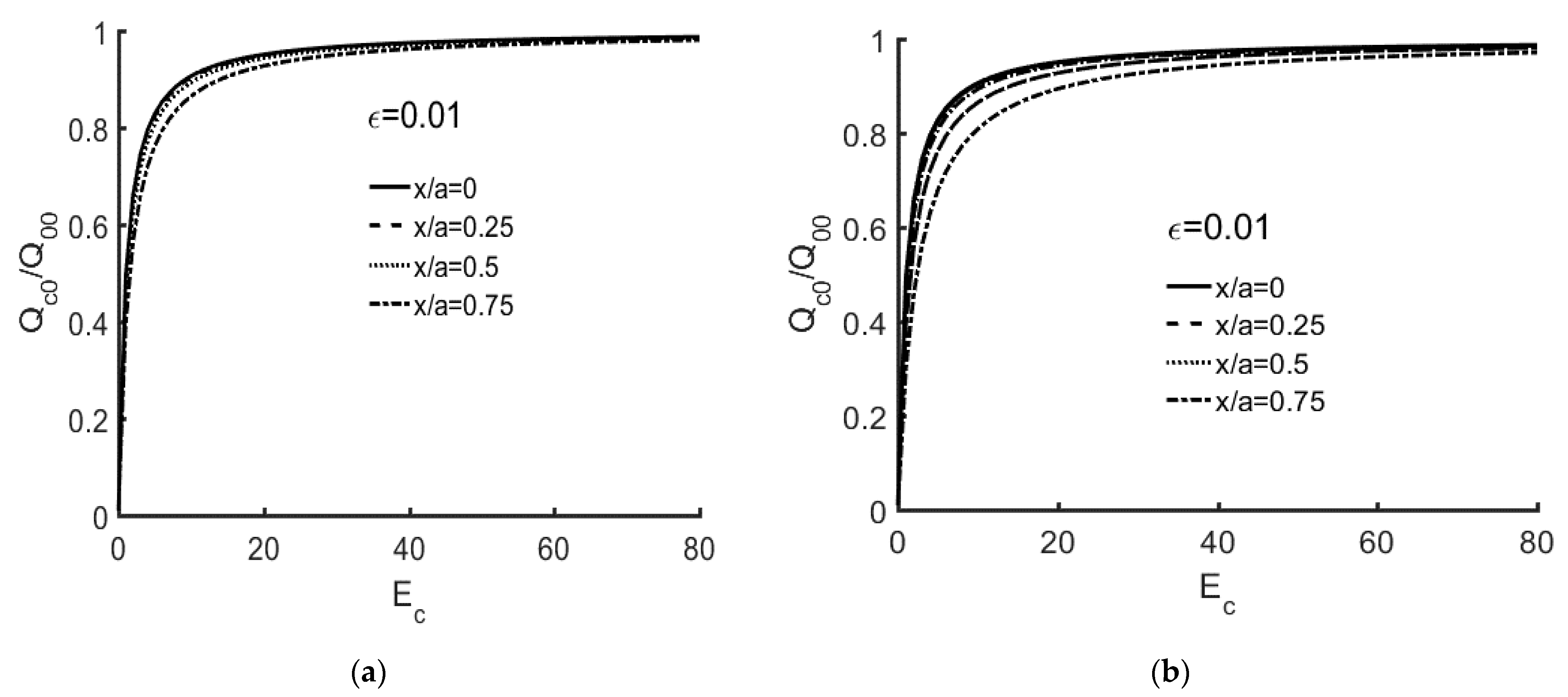
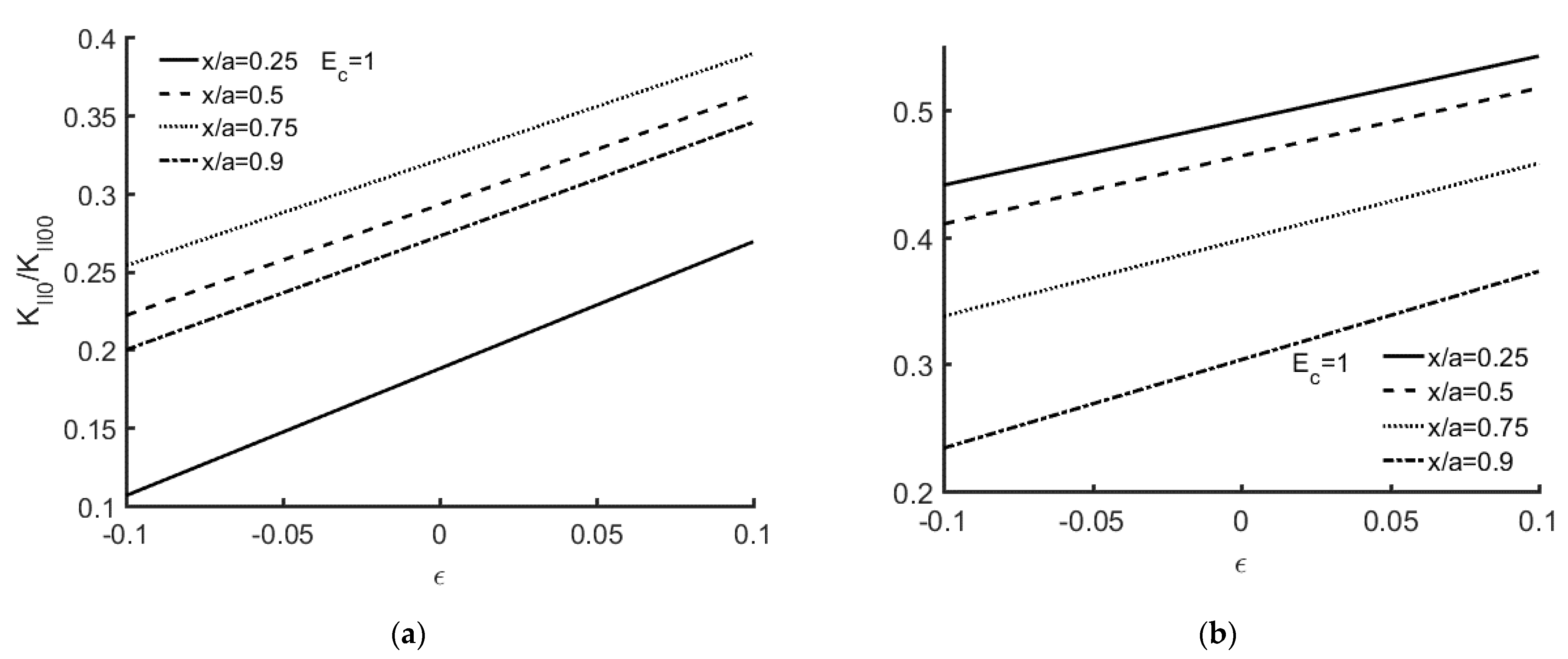
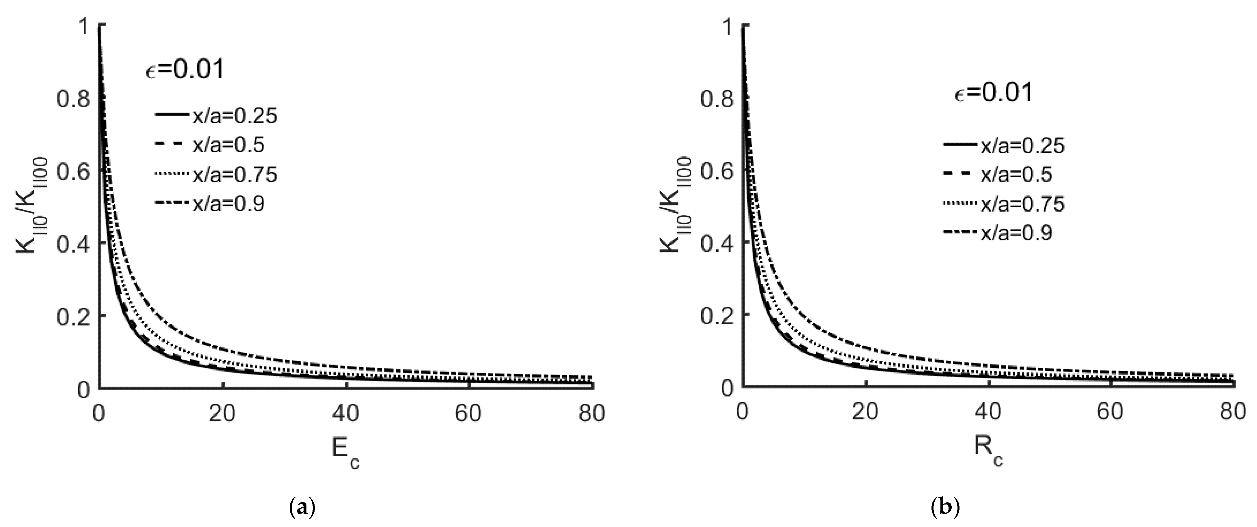
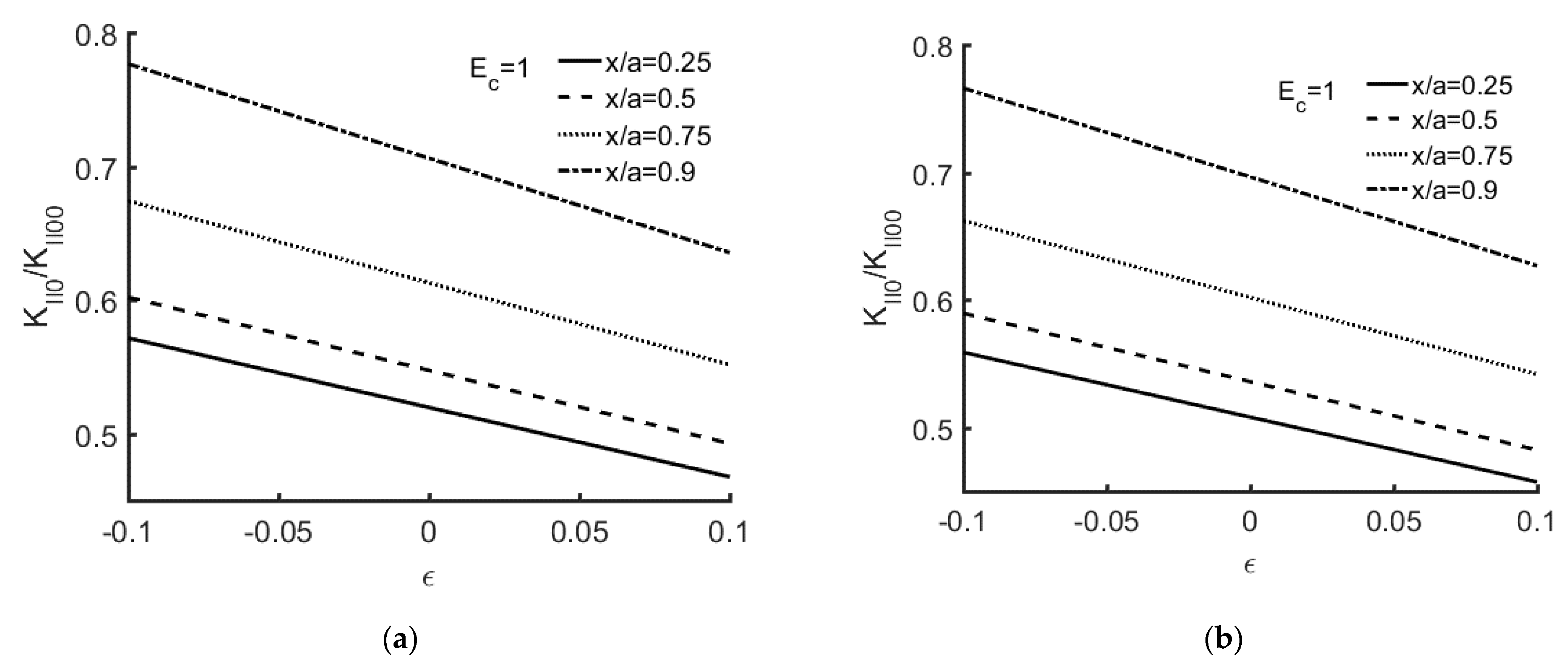
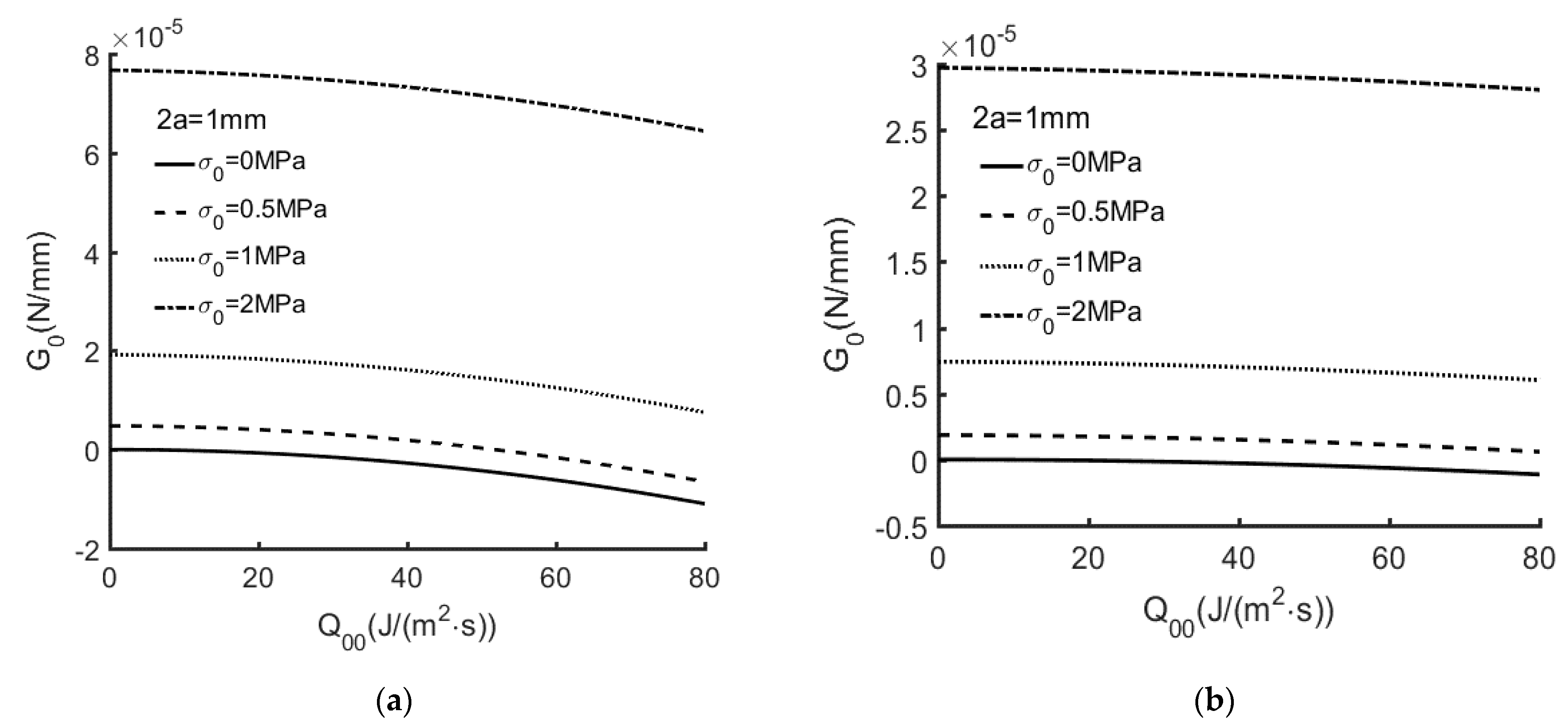
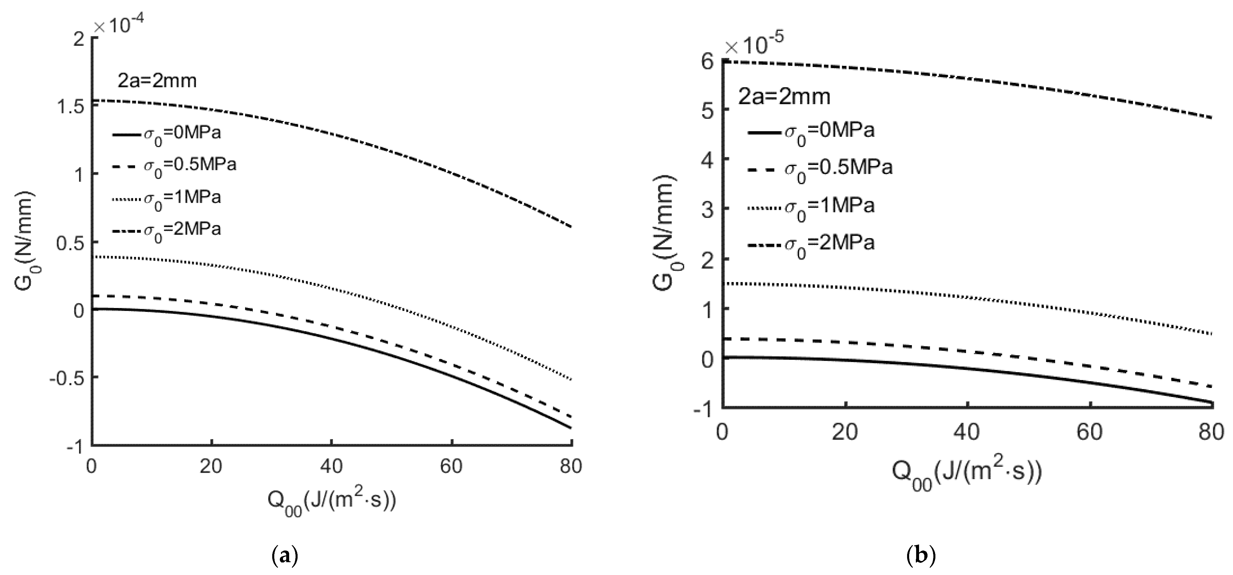
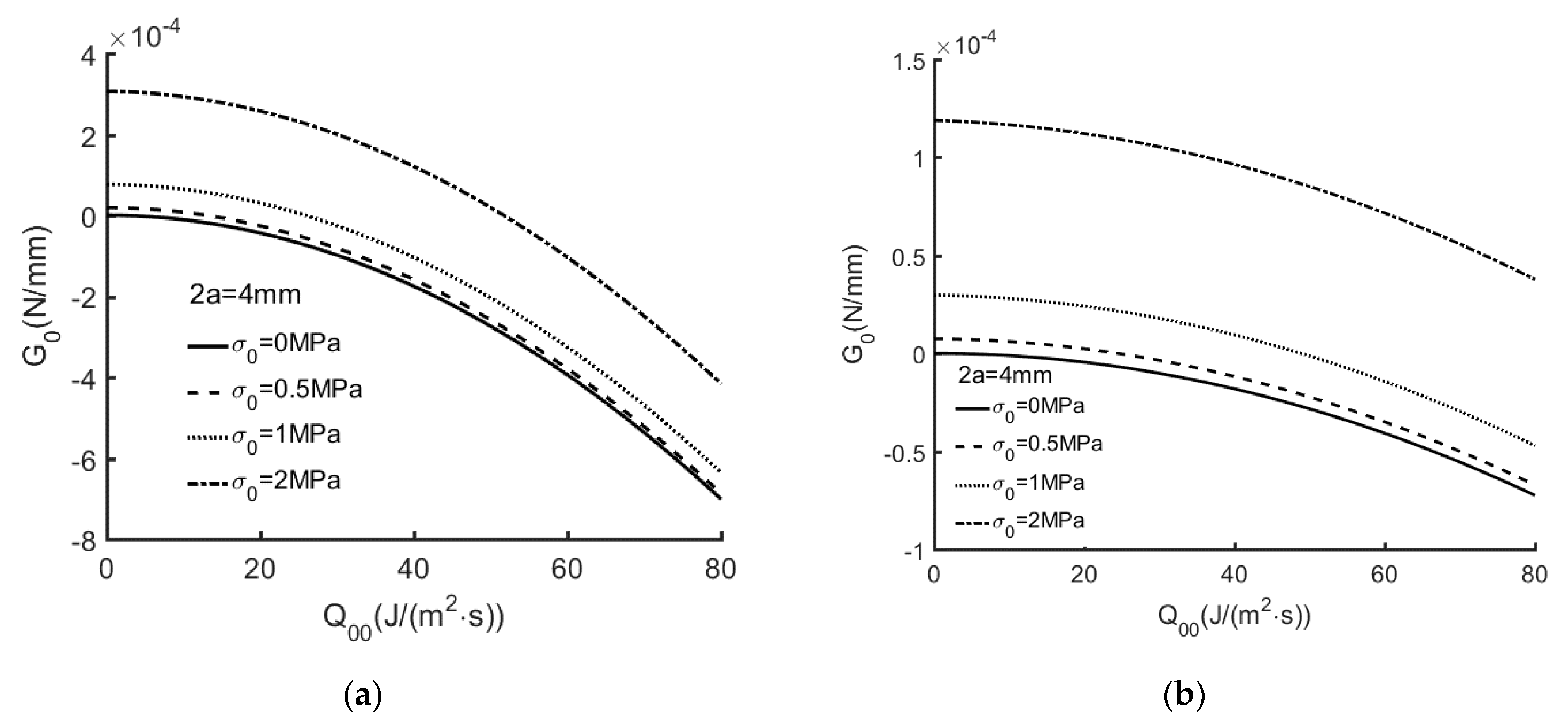
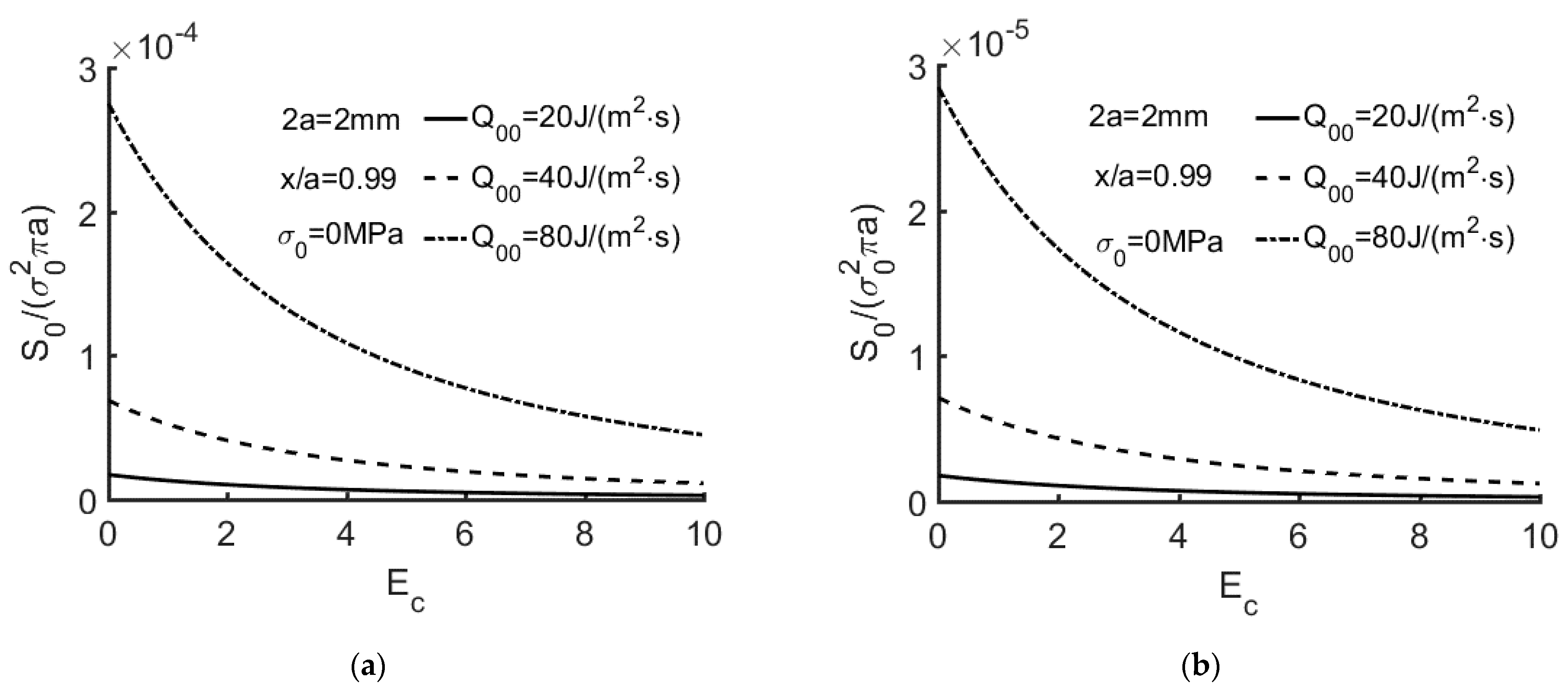
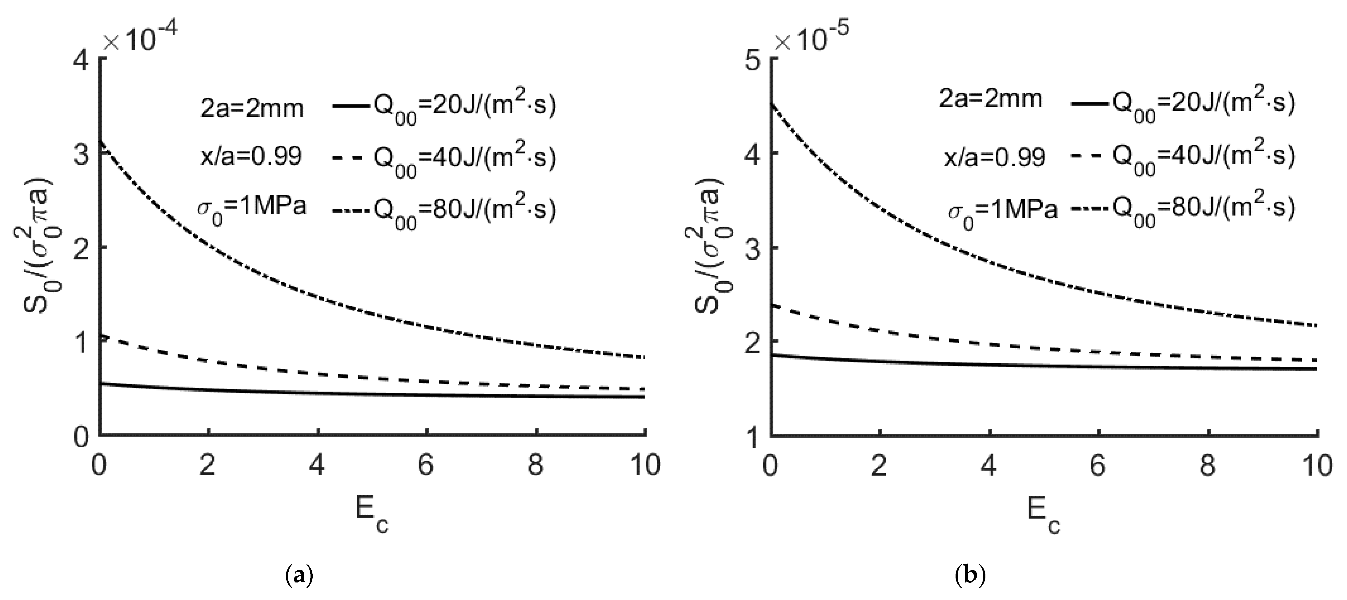
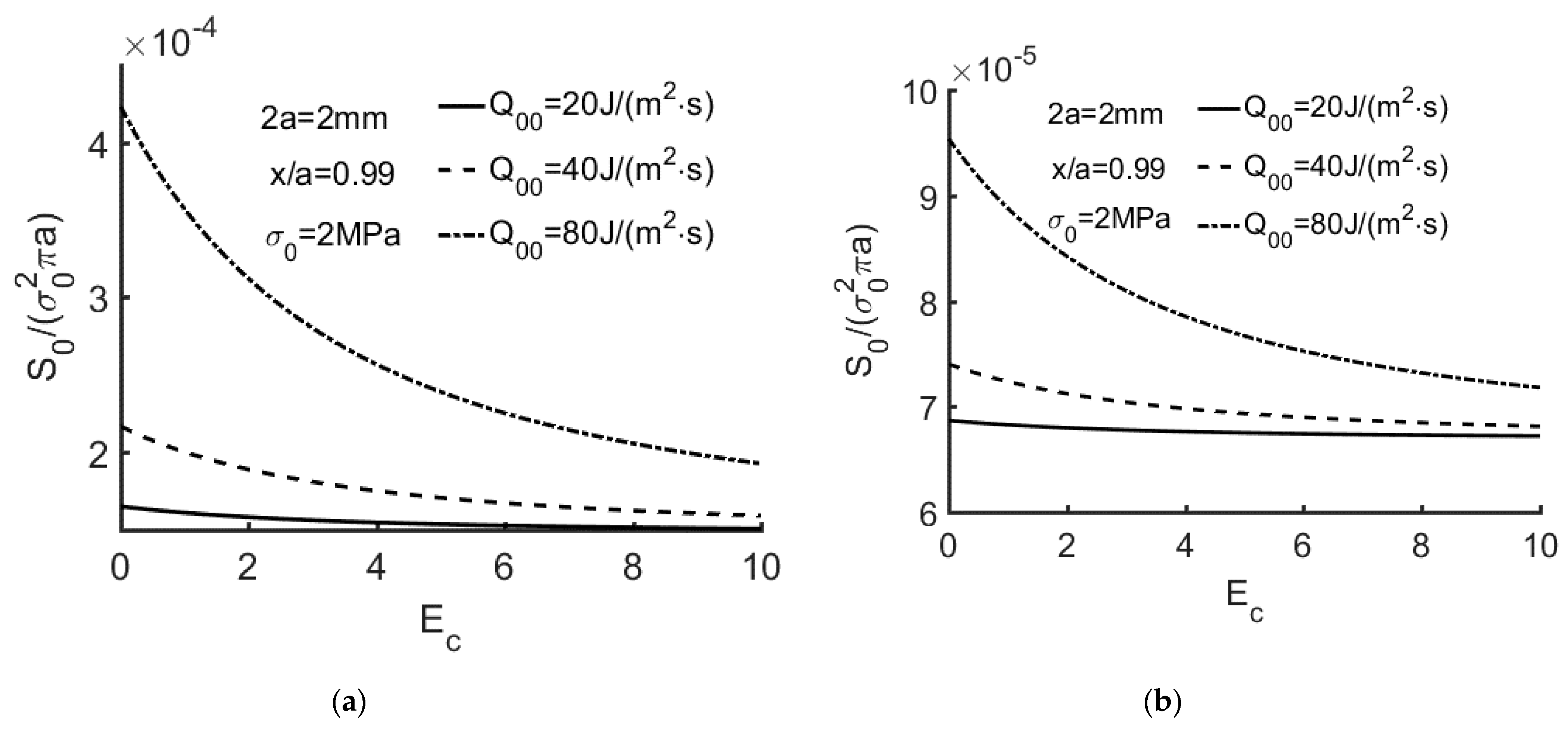
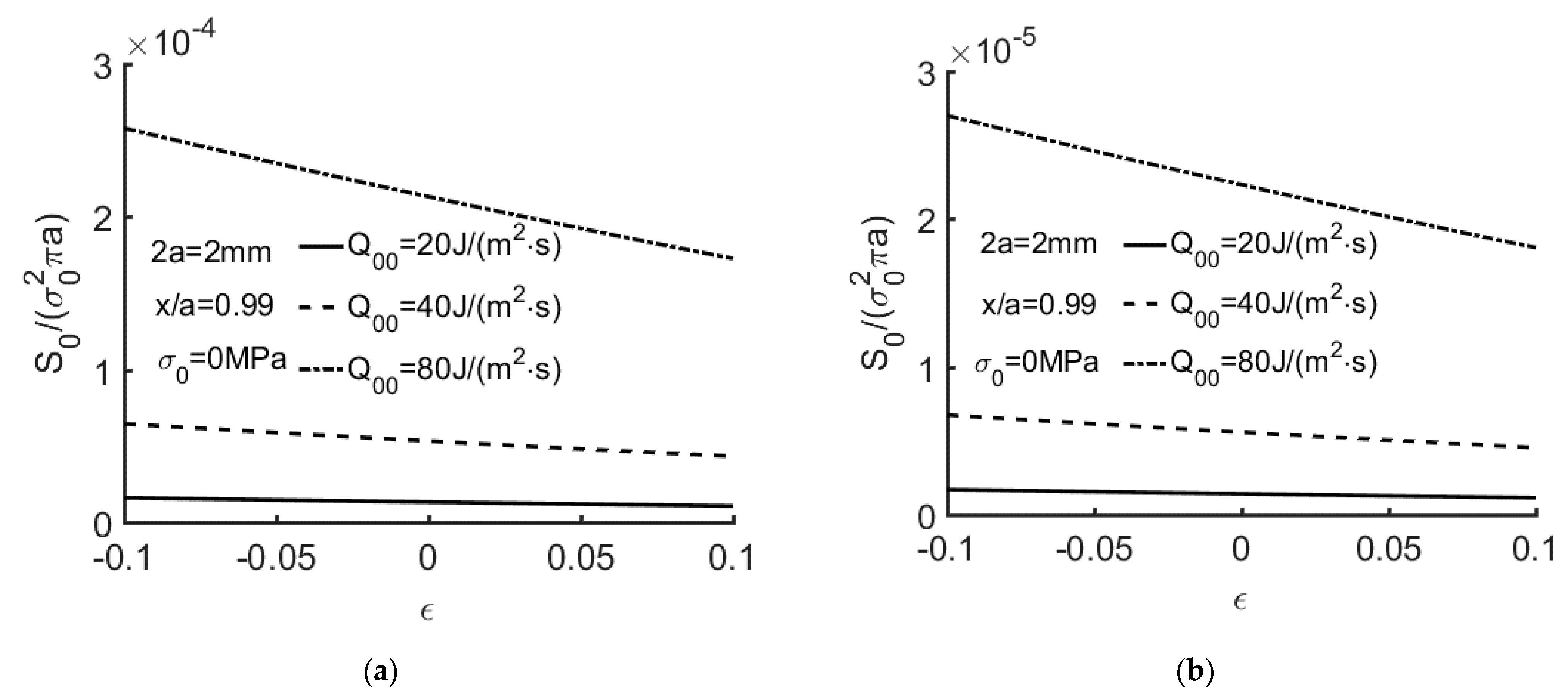
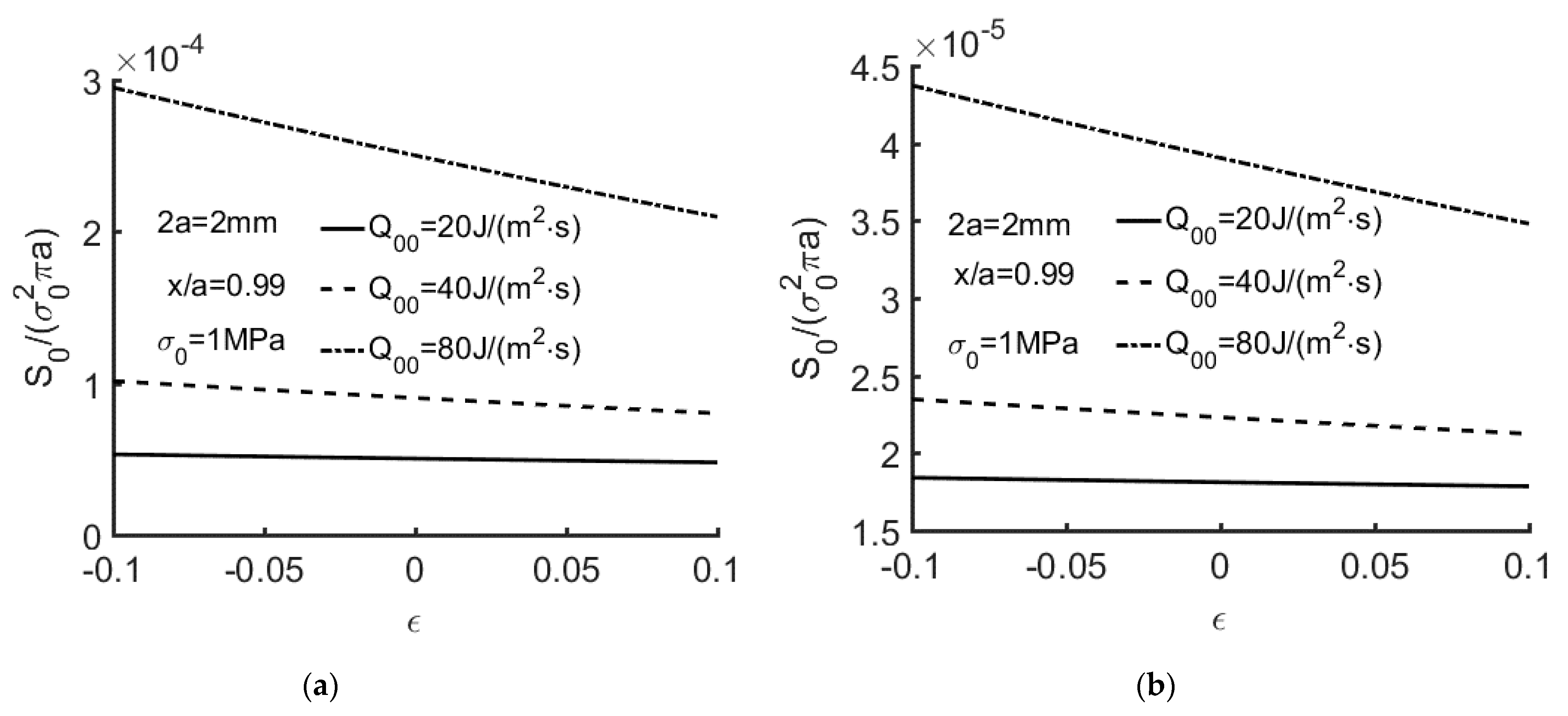
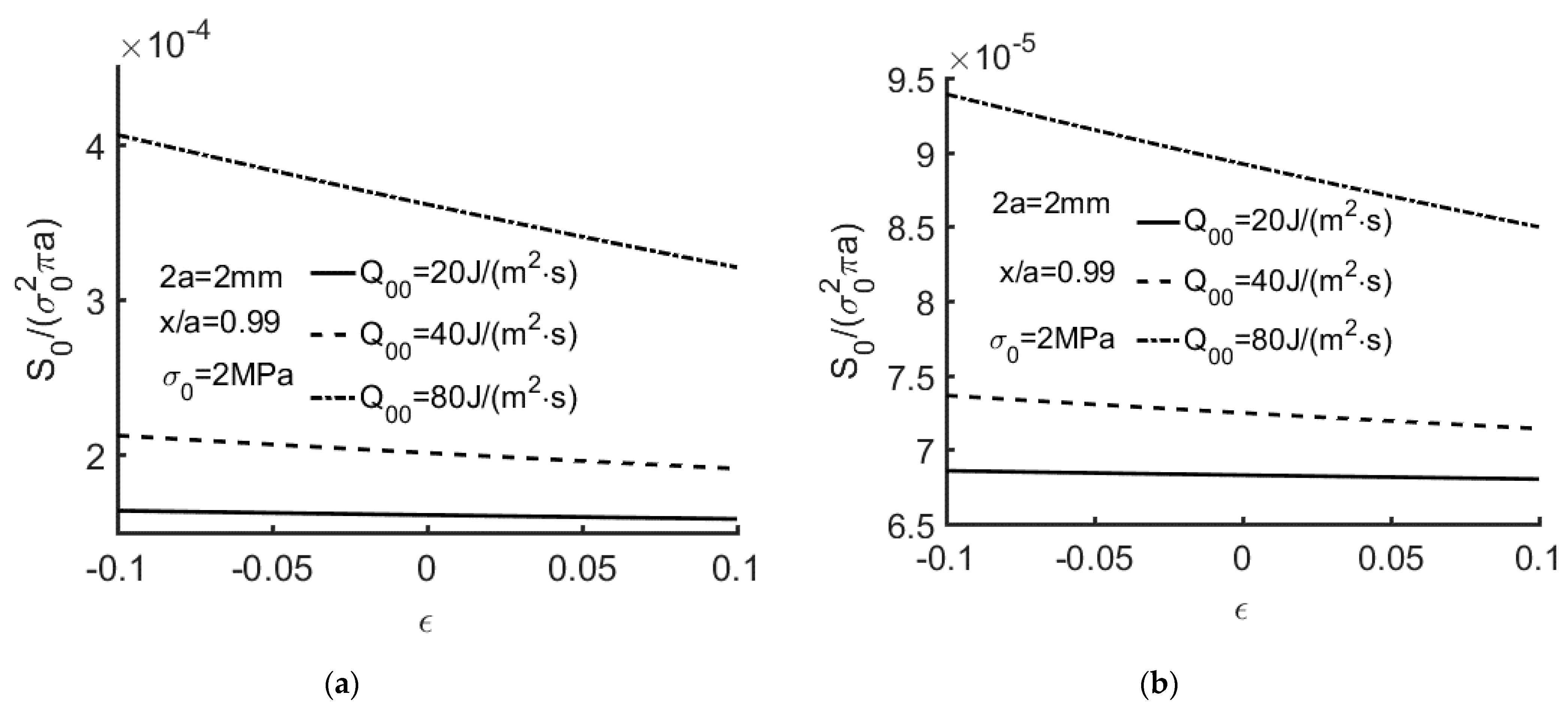
4. Numerical Results

In this section, we take the example of combined constant thermal flux and constant mechanical loading and research the influence of the constant thermo-mechanical loading, the dimensionless thermal resistance and the coefficient on the heat flux to the crack surface and the Mode-II SIF. The Mode-II SIF, the energy release rate (G) and the strain energy density factor on the crack line (S) under the constant thermal flux $-(Q_{00}-Q_{c0})/2a$ and the constant mechanical loading ${\sigma }_0$ are rewritten as $K_{II0}$, $G_0$, and $S_0$. The material constants of orthotropic and isotropic are listed in

Table 1. Material constants of Tyrannohex.

$\begin{array}{l}{\mathit{E}}_{\mathit{x}\mathit{x}}\\ (\mathit{G}\mathit{P}\mathit{a})\end{array}$	$\begin{array}{l}{\mathit{E}}_{\mathit{y}\mathit{y}}\\ (\mathit{G}\mathit{P}\mathit{a})\end{array}$	$\begin{array}{l}{\mathit{G}}_{\mathit{x}\mathit{y}}\\ (\mathit{G}\mathit{P}\mathit{a})\end{array}$	${\mathit{v}}_{\mathit{x}\mathit{y}}$	${\mathit{v}}_{\mathit{y}\mathit{x}}$	$\begin{array}{l}{\mathit{\alpha }}_{\mathit{x}\mathit{x}}\\ ({10}^{-5}{/}^0\mathit{C})\end{array}$	$\begin{array}{l} {\mathit{\alpha }}_{\mathit{y}\mathit{y}}\\ ({10}^{-5}{/}^0\mathit{C})\end{array}$	$\begin{array}{l}{\mathit{\lambda }}_{\mathit{x}}\\ (\mathit{w}/{\mathit{m}}^0\mathit{C})\end{array}$	$\begin{array}{l} {\mathit{\lambda }}_{\mathit{y}}\\ (\mathit{w}/{\mathit{m}}^0\mathit{C})\end{array}$
135	87	50	0.15	0.09667	0.32	0.32	3.08	2.81

and

Table 2. Constants of Steel.

$\begin{array}{l} {\mathit{E}}_{\mathit{x}\mathit{x}}\\ (\mathit{M}\mathit{P}\mathit{a})\end{array}$	$\begin{array}{l} {\mathit{E}}_{\mathit{y}\mathit{y}}\\ (\mathit{M}\mathit{P}\mathit{a})\end{array}$	$\begin{array}{l}{\mathit{G}}_{\mathit{x}\mathit{x}}\\ (\mathit{M}\mathit{P}\mathit{a})\end{array}$	${\mathit{v}}_{\mathit{x}\mathit{y}}$	${\mathit{v}}_{\mathit{y}\mathit{x}}$	$\begin{array}{l}{\mathit{\alpha }}_{\mathit{x}\mathit{x}}\\ ({10}^{-5}{/}^0\mathit{C})\end{array}$	$\begin{array}{l} {\mathit{\alpha }}_{\mathit{y}\mathit{y}}\\ ({10}^{-5}{/}^0\mathit{C})\end{array}$	$\begin{array}{l}{\mathit{\lambda }}_{\mathit{x}}\\ (\mathit{w}/{\mathit{m}}^0\mathit{C})\end{array}$	$\begin{array}{l} {\mathit{\lambda }}_{\mathit{y}}\\ (\mathit{w}/{\mathit{m}}^0\mathit{C})\end{array}$
205900	205900	79200	0.3	0.303	$1.14$	$1.14$	48.6	48.6

[31].

Figure 2a,b show $Q_{c0}/Q_{00}$ versus Ec with x/a = 0, 0.25, 0.5, 0.75 for $\epsilon$ = 0.01. It is easily seen that $Q_{c0}/Q_{00}$ increases with an increase of Ec for $\epsilon$ = 0.01. When Ec increases, it means that the heat flux per thickness to the crack surface increases. So, $Q_{c0}/Q_{00}$ increases. The constant $\epsilon$ is regarded as an adjustment physical quantity. The higher the value of constant $\epsilon$, the greater the heat flux per thickness to the crack surface. When Ec = 0 and $\epsilon$ = 0, we have $Q_{c0}=0$, which means a fully thermally impermeable crack. When Ec→∞, we have $Q_{c0}=Q_{00}$, which means a fully thermally permeable crack.

Figure 3a,b show Q_c0/Q₀₀ versus $\epsilon$ with x/a = 0, 0.25, 0.5, 0.75 for Ec = 1. It is easily seen that the variations of Q_c0/Q₀₀ increase with an increase of $\epsilon$ for Ec = 1. From Figure 2 to Figure 3, the case Ec = 1 correlates with the situation that the crack region is identical to that of the orthotropic material. The cases Ec = 2, Ec = 3, and Ec = 4 indicate that the heat conduction is one, two and three times stronger than thermal conductivity of the orthotropic material respectively. The case with Ec = 0 and $\epsilon$ = 0 corresponds to the thermally impermeable and the case with Ec→∞ corresponds to the thermally impermeable.

Figure 4a,b display K_II0/K_II00 versus Ec, where K_II0 represents K_I00 when Q_c0 = 0 and $\epsilon$ = 0. It is easily seen that K_II0/K_II00 decreases with an increase of Ec for $\epsilon$ = 0.01.

Figure 5a,b display K_II0/K_II00 versus $\epsilon$. It is easily seen that the K_II0/K_II00 decreases with an increase of Ec and $\epsilon$, respectively).

Figure 6, Figure 7 and Figure 8 show G₀, as computed using Equation (89), for the extended partially insulated crack (E_c = 0, $\epsilon$ = 0) with a variety of thermal flux and crack lengths. With the increase of crack length, the thermal flux around the crack surface increases. It means that the value of energy release rate increases with the increase of the shearing stress and shear displacement induced by the thermal flux. When thermal flux outweighs remote tensile stress, the value of G₀ may turn negative.

Figure 9, Figure 10 and Figure 11 show S₀/(σ₀²πa) versus E_c for the extended partially insulated crack ($\epsilon$ = 0.01) with a variety of thermal flux. It is found that S₀/(σ₀²πa), as computed using Equation (92), decreases with E_c.

Figure 12, Figure 13 and Figure 14 show S₀/(σ₀²πa) for the extended partially insulated crack (E_C = 1) with a variety of thermal flux. From Equation (92), S₀/(σ₀²πa) consist of the mode-I stress intensity factor induced by thermal flux and the mode-II stress intensity factor created by mechanical loading. When thermal flux and mechanical loading increase, the corresponding intensity factors and S₀/(σ₀²πa) increase. It is revealed that crack face boundary conditions have a great effect on strain energy density factor on the crack line based on numerical results.

5. Conclusions

This paper presents a detailed study into the fracture analysis for a crack in orthotropic material subjected to combined 2i-order symmetrical thermal flux and 2j-order symmetrical mechanical loading. As the closed form solutions of main fracture parameters have been obtained, it provides a quick and convenient way to solve predicting the remaining life of above problems.

The analysis presented in this paper has also revealed that, for a given mechanical load, the presence of thermal loads can induce the energy release rate to become either negative or positive, depending on the relative magnitude of the thermal loads and the crack surface conditions of impermeability. In contrast, the strain energy density ahead of the crack is always positive. This finding should not be taken to infer that energy release rate approaches should be avoided when assessing structural integrity, merely that only the positive excursion of G should be used to assess delamination growth. This recommendation mimics the approach commonly used to assess crack growth in metals, where only the positive excursion of K is used to compute crack growth.

References

1. Nowacki, W. Thermoelasticity; Pergamon Press: New York, NY, USA, 1962. [Google Scholar]
2. Sih, G.C.; Michaopoloulos, J.; Chou, S.C. Hygrothermoelasticity; Martinus Niijhoof Publishing: Leiden, The Netherlands, 1986. [Google Scholar]
3. Nowinski, J.L. Theory of Thermoelasticity with Applications; Sijthoff and Noordhoff: Amsterdam, The Netherlands, 1978. [Google Scholar]
4. Sih, G.C. Thermomechanics of solids: Non-equilibrium and irreversibility. Theor. Appl. Fract. Mec. 1988, 9, 175–198. [Google Scholar] [CrossRef]
5. Olesiak, Z.; Sneddon, I.N. The distribution of thermal stress in an infinite elastic solid containing a penny-shaped crack. Arch. Ration. Mech. Anal. 1959, 4, 238–254. [Google Scholar] [CrossRef]
6. Fabrikant, V.I. Mixed Boundary Value Problem of Potential Theory and Their Applications in Engineering; Kluwer Academic Publishers: Dordrecht, The Netherlands, 1991. [Google Scholar]
7. Fabrikant, V.I. Complete solution to the problem of an external circular crack in a transversely isotropic body subjected to arbitrary shear loading. Int. J. Solids. Struct. 1996, 33, 167–191. [Google Scholar] [CrossRef]
8. Georgiadis, H.G.; Brock, L.M.; Rigatos, A.P. Transient concentrated thermal/mechanical loading of the faces of a crack in a coupled-thermoelastic solid. Int. J. Solids. Struct. 1998, 35, 1075–1097. [Google Scholar] [CrossRef]
9. Sih, G.C. On the singular character of thermal stress near a crack tip. J. Appl. Mech. 1962, 29, 587–589. [Google Scholar] [CrossRef]
10. Tsai, Y.M. Orthotropic thermoelastic problem of uniform heat flow disturbed by a central crack. J. Compos. Mater. 1984, 18, 122–131. [Google Scholar] [CrossRef]
11. Chen, B.X.; Zhang, X.Z. Thermoelasticity problem of an orthotropic plate with two collinear cracks. Int. J. Fract. 1988, 38, 161–192. [Google Scholar]
12. Wilson, W.K.; Yu, I.W. The use of J-integral in thermal stress crack problems. Int. J. Fract. 1979, 15, 377–387. [Google Scholar]
13. Prasad, N.N.V.; Aliabaid, M.H. The dual boundary element method for transient thermoelastic crack problems. Int. J. Solids Struct. 1996, 33, 2695–2718. [Google Scholar] [CrossRef]
14. Yang, J.; Jin, X.Y.; Jin, N.G. A penny-shaped crack in an infinite linear transversely isotropic triple medium subjected to uniform anti-symmetric heat flux: Closed-form solution. Eur. J. Mech. A Solids 2014, 47, 254–270. [Google Scholar] [CrossRef]
15. Hu, K.Q.; Chen, Z.T. Thermoelastic analysis of a partially insulated crack in a strip under thermal impact loading using the hyperbolic heat conduction theory. Int. J. Eng. Sci. 2012, 51, 144–160. [Google Scholar] [CrossRef]
16. Hu, K.Q.; Chen, Z.T. Transient heat conduction analysis of a cracked half-plane using dual-phase-lag theory. Int. J. Heat Mass Transf. 2013, 62, 445–451. [Google Scholar] [CrossRef]
17. Brock, L.M. Reflection and diffraction of plane temperature-step waves in orthotropic thermoelastic solids. J. Therm. Stresses 2010, 33, 879–904. [Google Scholar] [CrossRef]
18. Wu, B.; Zhu, J.G.; Peng, D. Thermoelastic analysis for two collinear cracks in an orthotropic solid disturbed by anti-symmetrical linear heat flow. Math. Probl. Eng. 2017, 10, 1–10. [Google Scholar]
19. Wu, B.; Peng, D.; Jones, R. The analysis of cracking under a combined quadratic thermal flux and a quadratic mechanical loading. Appl. Math. Model. 2019, 68, 182–197. [Google Scholar] [CrossRef]
20. Rekik, M.; Neifar, M.; El-Borgi, S. An axisymmetric problem of a partially insulated crack embedded in a graded layer bonded to a homogeneous half-space under thermal loading. J. Therm. Stresses 2011, 34, 201–227. [Google Scholar] [CrossRef]
21. Yang, W.; Pourasghar, A.; Chen, Z. Thermoviscoelastic fracture analysis of a cracked orthotropic fiber reinforced composite strip by the dual-phase-lag theory. Compos. Struct. 2021, 258, 113194. [Google Scholar] [CrossRef]
22. Pourasghar, A.; Chen, Z. Dual-phase-lag heat conduction in the composites by introducing a new application of DQM. Heat Mass Transf. 2020, 56, 1171–1177. [Google Scholar] [CrossRef]
23. Kuo, A.Y. Effects of crack surface heat conductance on stress intensity factors. Math. Probl. Eng. 1990, 57, 354–358. [Google Scholar] [CrossRef]
24. Lee, Y.D.; Erdogan, F. Interface cracking of FGM coatings under steady-state heat flow. Eng. Fract. Mech. 1998, 59, 361–380. [Google Scholar] [CrossRef]
25. Lee, K.Y.; Park, S.J. Thermal stress intensity factors for partially insulated interface crack under uniform heat flow. Eng. Fract. Mech. 1995, 50, 475–482. [Google Scholar] [CrossRef]
26. Zhou, Y.T.; Li, X.; Yu, D.B. A partially insulated interface crack between a graded orthotropic coating and a homogeneous orthotropic substrate under heat flux supply. Int. J. Solids Struct. 2010, 47, 768–778. [Google Scholar] [CrossRef] [Green Version]
27. Zhong, X.C. Closed-form solutions for two collinear dielectric crack in mageto-electroelastic solid. Appl. Math. Model. 2011, 35, 2930–2944. [Google Scholar] [CrossRef]
28. Wu, B. Closed-Form Solutions of Cracked Elastic Solids under a Combined Thermal Flux and a Mechanical Loading and Application. Ph.D. Thesis, HHu, Nanjing, China, 2019. [Google Scholar]
29. Gradshteyn, I.S.; Ryzhik, I.M. Table of Integrals, Series, and Products; Elsevier Academic Press: Cambridge, MA, USA, 2007. [Google Scholar]
30. Sih, G.C. Mechanics of Fracture Initiation and Propagation; Kluwer Academic Publishers: Boston, MA, USA, 1991. [Google Scholar]
31. Itou, S. Thermal stress intensity factors of an infinite orthotropic layer with a crack. Int. J. Fract. 2000, 103, 279–291. [Google Scholar] [CrossRef]
Figure 1. A single crack which is embedded in an orthotropic solid subjected to combined 2i order polynomial function thermal flux and 2j order polynomial function mechanical loading.
Applmech 02 00008 g001
Figure 2. (a) Qc0/Q00 versus Ec with x/a = 0, 0.25, 0.5, 0.75 for ε = 0.01. The orthotropic material listed in Table 1; (b) Qc0/Q00 versus Ec with x/a = 0, 0.25, 0.5, 0.75 for ε = 0.01. The isotropic material listed in Table 2.
Applmech 02 00008 g002
Figure 3. (a) Qc0/Q00 versus ε with x/a = 0.25, 0.5, 0.75, 0.9 for Ec = 1. The orthotropic material listed in Table 1; (b) Qc0/Q00 versus ε with x/a = 0, 0.25, 0.5, 0.75 for Ec = 1. The isotropic material listed in Table 2.
Applmech 02 00008 g003
Figure 4. (a) KII0/KI00 versus Ec with x / a = 0.25, 0.5, 0.75, 0.9 for ε = 0.01. The orthotropic material listed in Table 1; (b) KII0/KI00 versus Ec with x / a = 0.25, 0.5, 0.75, 0.9 for ε = 0.01. The isotropic material listed in Table 2.
Applmech 02 00008 g004
Figure 5. (a) KII0/KII00 versus ε with x/a = 0.25, 0.5, 0.75, 0.9 for Ec = 1 The orthotropic material listed in Table 1; (b) KII0/KII00 versus ε with x/a = 0.25, 0.5, 0.75, 0.9 for Ec = 1. The isotropic material listed in Table 2.
Applmech 02 00008 g005
Figure 6. (a) G0 versus tension stress with σ0 = 0, 0.5, 1, 2 MPa for Ec = 0, ε = 0, 2a = 1 mm. The orthotropic material listed in Table 1; (b) G0 versus tension stress with σ0 = 0, 0.5, 1, 2 MPa for Ec = 0, ε = 0, 2a = 1 mm. The isotropic material listed in Table 2.
Applmech 02 00008 g006
Figure 7. (a) G0 versus tension stress with σ0 = 0, 0.5, 1, 2 MPa for Ec = 0, ε = 0. (2a = 2 mm). The orthotropic material listed in Table 1. (b) G0 versus tension stress with σ0 = 0, 0.5, 1, 2 MPa for Ec = 0, ε = 0. (2a = 2 mm). The isotropic material listed in Table 2.
Applmech 02 00008 g007
Figure 8. (a) G0 versus tension stress with σ0 = 0, 0.5, 1, 2 MPa for Ec = 0, ε = 0. (2a = 4 mm). The orthotropic material listed in Table 1. (b) G0 versus tension stress with σ0 = 0, 0.5, 1, 2 MPa for Ec = 0, ε = 0. (2a = 4 mm). The isotropic material listed in Table 2.
Applmech 02 00008 g008
Figure 9. (a) S0/(σ02πa) versus Ec with Q00 = 20, 40, 80 J/(m2·s) for ε = 0.01. (2a = 2 mm, x/a = 0.99, σ0 = 0 MPa). The orthotropic material listed in Table 1. (b) S0/(σ02πa) of versus Ec with Q00 = 20, 40, 80 J/(m2·s) for ε = 0.01. (2a = 2 mm, x/a = 0.99, σ0 = 0 MPa). The isotropic material listed in Table 2.
Applmech 02 00008 g009
Figure 10. (a) S0/(σ02πa) versus Ec with Q00 = 20, 40, 80 J/(m2·s) for ε = 0.01. (2a = 2 mm, x/a = 0.99, σ0 = 2 MPa). The orthotropic material listed in Table 1. (b) S0/(σ02πa) versus Ec with Q00 = 20, 40, 80 J/(m2·s) for ε = 0.01 (2a = 2 mm, x/a = 0.99, σ0 = 1 MPa). The isotropic material listed in Table 2.
Applmech 02 00008 g010
Figure 11. (a) S0/(σ02πa) versus Ec with Q00 = 20, 40, 80 J/(m2·s) for ε = 0.01. (2a = 2 mm, x/a = 0.99, σ0 = 2 MPa). The orthotropic material listed in Table 1. (b) S0/(σ02πa) versus Ec with Q00 = 20, 40, 80 J/(m2·s) for ε = 0.01. (2a = 2 mm, x/a = 0.99, σ0 = 2 MPa). The isotropic.
Applmech 02 00008 g011
Figure 12. (a) S0/(σ02πa) versus ε with Q00 = 20, 40, 80 J/(m2·s) for Ec = 1. (2a = 2 mm, x/a = 0.99, σ0 = 0 MPa). The orthotropic material listed in Table 1. (b) S0/(σ02πa) versus ε with Q00 = 20, 40, 80 J/(m2·s) for Ec = 1. (2a = 2 mm, x/a = 0.99, σ0 = 0 MPa). The isotropic material listed in Table 2.
Applmech 02 00008 g012
Figure 13. (a) S0/(σ02πa) versus ε with Q00 = 20, 40, 80 J/(m2·s) for Ec = 1. (2a = 2 mm, x/a = 0.99, σ0 = 1 MPa). The orthotropic material listed in Table 1. (b) S0/(σ02πa) versus ε with Q00 = 20, 40, 80 J/(m2·s) for Ec = 1. (2a = 2 mm, x/a = 0.99, σ0 = 1 MPa). The isotropic material listed in Table 2.
Applmech 02 00008 g013
Figure 14. (a) S0/(σ02πa) versus ε with Q00 = 20, 40, 80 J/(m2·s) for Ec = 1. (2a = 2 mm, x/a = 0.99, σ0 = 2 MPa). The orthotropic material listed in Table 1. (b) S0/(σ02πa) versus ε with Q00 = 20, 40, 80 J/(m2·s) for Ec = 1. (2a = 2 mm, x/a = 0.99, σ0 = 2 MPa). The isotropic material listed in Table 2.
Applmech 02 00008 g014