Person Identification by Footstep Sound Using Convolutional Neural Networks


German Aerospace Center (DLR), Lilienthalplatz 7, 38108 Braunschweig, Germany
*
Author to whom correspondence should be addressed.
Appl. Mech. 2021, 2(2), 257-273; https://0-doi-org.brum.beds.ac.uk/10.3390/applmech2020016
Submission received: 13 April 2021
/
Revised: 27 April 2021
/
Accepted: 27 April 2021
/
Published: 11 May 2021
(This article belongs to the Special Issue Smart Structures and Systems: Actual Scientific and Industrial Research)
Abstract
:Human gait is very individual and it may serve as biometric to identify people in camera recordings. Comparable results can be achieved while using the acoustic signature of human footstep sounds. This acoustic solution offers the opportunity of less installation space and the use of cost-efficient microphones when compared to visual system. In this paper, a method for person identification based on footstep sounds is proposed. First, step sounds are isolated from microphone recordings and separated into 500 ms samples. The samples are transformed with a sliding window into mel-frequency cepstral coefficients (MFCC). The result is represented as an image that serves as input to a convolutional neural network (CNN). The dataset for training and validating the CNN is recorded with five subjects in the acoustic lab of DLR. These experiments identify a total number of 1125 steps. The validation of the CNN reveals a minimum -score of 0.94 for all five classes and an accuracy of 0.98. The Grad-CAM method is applied to visualize the background of its decision in order to verify the functionality of the proposed CNN. Subsequently, two challenges for practical implementations, noise and different footwear, are discussed using experimental data.
1. Introduction
Human gait is a complex process that involves the entire locomotor system. As a consequence, it is affected by many factors, like diseases, injuries, and age, just to mention a few [1]. Gait analysis is a discipline that studies the walking process of subjects in order to reveal these factors. Since the gait is very individual, not only medical professionals are interested in its analysis. Security research recognized the opportunity to use the walking behavior as a biometric [2]. Progressing computer performance allowed for complex image processing tasks. Gait analysis now offers person identification using a biometric that is recorded from a distance by surveillance cameras, for example.
Not only can vision systems identify individuals by their gait, but humans themselves are able to recognize others in their workplace, e.g., by means of visual and aural perception [3]. Even without visual information, humans are still able to identify a passerby in front of their office door only by its walking sound. Individual training may enhance the performance of recognition.
Person identification using only walking sound includes some advantages. It requires less complex and expensive hardware than visual systems. Difficult coverage, illumination, and view angle are just a few difficulties that are associated with the use of cameras. Sound, on the other hand, propagates freely in the air, and the position of the microphone can be selected less strictly.
An acoustic gait analysis to extract parameters for medical purposes is presented in [4]. The authors are able to extract the quantitative characteristics of human gait by using audio signals from a recording room. Further studies are foreseen to apply this technique in clinical conditions. In contrast to the preceding non-intrusive measurement, the authors in [5] work with wearable microphones to record the walking sound of individuals. Data analysis is performed with an external laptop.
Nevertheless, walking sounds are complex audio signals. Simple time signal recording and comparison cannot reveal the identity of the walker. Variations of walking sound from step-to-step are rather high. The human ear and brain are able to distinguish individuals. Therefore, neural networks seem to be ideally suited to solve this issue and identify a walker. In fact, neural networks have been discovered for this application in recent years [6,7,8,9,10]. The increasing capability of convolutional neural networks make them popular in machine learning applications. Deep learning facilitates the training of CNN with high numbers of layers and parameters. The origin of the CNN lies in image recognition tasks. Nets, like VGG16/19 [11], AlexNet [12], or DenseNet [13], are able to classify images with human-like performance.
This performance led to a trend of reformulating non-image based problems into image-based ones. Bird song recordings are transformed into spectrograms in [14,15]. The species are determined with high accuracy by using image recognition CNN on the spectrograms. Comparable approaches have been made to recognize speakers [16,17] and their emotion [17,18]. Auditory information allows humans to recognize their environment and react to events. The same functionality is transferred to machine learning using CNN. Numerous challenges, like Detection and Classification of Acoustic Scenes and Events (DCASE) (dcase.community), provide tasks for event and scene recognition based on audio recordings. In many cases these tasks are solved by the use of CNN [17,19,20,21,22].
In this paper, the objective is to identify walking subjects based on single microphone recordings of airborne sound. The focus lies on the recognition of step sound. Here, step sound is treated as a subset of walking sound. Walking sound includes all sounds that are emitted by a walking person. Sources may be clothing, backpacks, handbags, etc. Furthermore, the selection of step sound for recognition gives the opportunity to neglect the walking speed or step frequency, respectively. Additionally, the process of running is excluded from analysis by defining that at least one foot must contact the ground [1].
In medicine, the human gait is defined as a gait cycle subdivided into seven events. It begins when the heel of a foot has initial contact to the ground and it ends when the same foot touches the ground again. One cycle is divided into a stance and a swing phase. The stance phase begins with the initial contact of the heel and it remains as long as the foot is in contact with the ground. During the swing phase, the foot swings back and forward until the heel touches the ground again. From an acoustical point of view, the stance phase is of interest, since the footstep sound is emitted here. The human ear usually perceives only a single impact sound when the foot touches the ground. However, recordings of step sounds reveal that it consists of three subsequent impacts [1,4]. The initial contact of the heel leads to the heelstrike transient. It is followed by the mid-stance peak when the metatarso-phalangeal (MTP) joints hit the ground. The terminal stance or so-called toe-off event concludes the step sound. The characteristic of these three acoustic events is very individual and it may serve as a kind of biometric for person identification. For practical implementations, additional filtering of the step sounds by footwear, injuries, additional weight, or floor type, e.g., have to be considered.
The first section of this article describes the recording of experimental data in the acoustic lab of DLR. The recordings are pre-processed and transformed into images for the use in an input layer of a CNN. Afterwards, the setup and the training of the CNN is described in detail. In order to obtain the performance of the proposed CNN, it is applied to the validation dataset. Because CNN are like black boxes, a class activation mapping algorithm is used afterwards to gain insight in the functionality of the net. Two challenges in practical applications, noise and different footwear, are investigated in the final section.
2. Experiment
2.1. Setup
Footsteps are relatively quiet sound events as compared to other urban or indoor sounds. Measurements are conducted in the acoustic transmission loss test facility (ATB) of DLR in order to create a low noise database of footstep sounds. One part of the ATB is a semi-anechoic room with a lower cut-off frequency of 100 Hz, which complies to DIN EN ISO 3745. With its inner dimensions of 5.8 × 3.5 m2 and its sealed concrete floor, it is ideally suited for walking experiments. The setup consists of a single microphone of type T130D21 from PCB® elastically mounted on the floor in vertical direction. Around the microphone, a circle with app. 2 m diameter is marked on the floor as guidance for the subjects. The circular path ensures a constant distance to the microphone and, therefore, a constant mean sound pressure level (SPL). For the recordings, a NoisePAD™ from Sinus Messtechnik GmbH is used. The audio signals are recorded with 51.2 kHz sampling rate and 24 bit resolution. The recordings are saved without compression to preserve signal quality.
2.2. Measurement
Five subjects (one female, four male) took part in the experiment. Each subject was requested to walk the circular path for 60 s clockwise (CW). Afterwards, the measurement was repeated in counter-clockwise (CCW) direction. While walking clockwise, the right foot is closer to the microphone than the left one. Additionally, individual walking behaviour may lead to differences between inner and outer foot. Walking in both directions averages these effects and enables the recording of a consistent database.
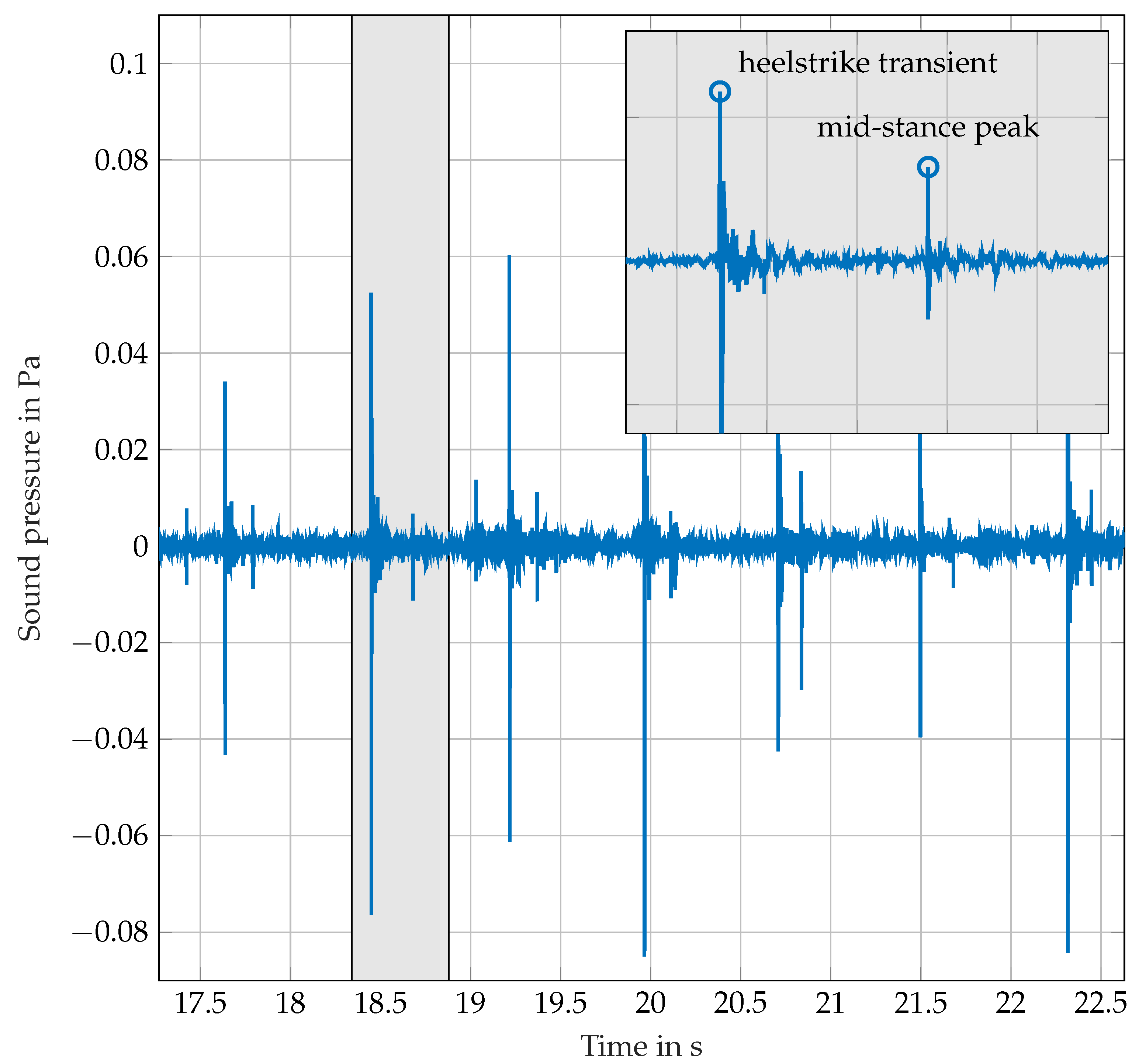
A total of 14 measurements were conducted, which are summarized in Table 1. For further tests, two subjects (1 & 4) changed their footwear and repeated walking. In measurements M03-06 additional squeaking of the footwear occurred during some steps. Figure 1 shows an example of the recorded signals. Here, seven steps from M13 are plotted. The second step is magnified and the heelstrike transient and the mid-stance peak are clearly identifiable. A toe off event cannot be unambiguously determined. Subject 5 was wearing shoes with rather stiff soles which lead to a distinct step sound. The SPL of the heelstrike transients in M13 reached up to 77 dB. In all measurements, only the direct sound was recorded. No echoes could be observed because of the anechoic environment. The magnified single step in Figure 1 has a length of 536 ms. The duration of a typical acoustic step event in the recordings is around 500 ms.
3. Data Pre-Processing
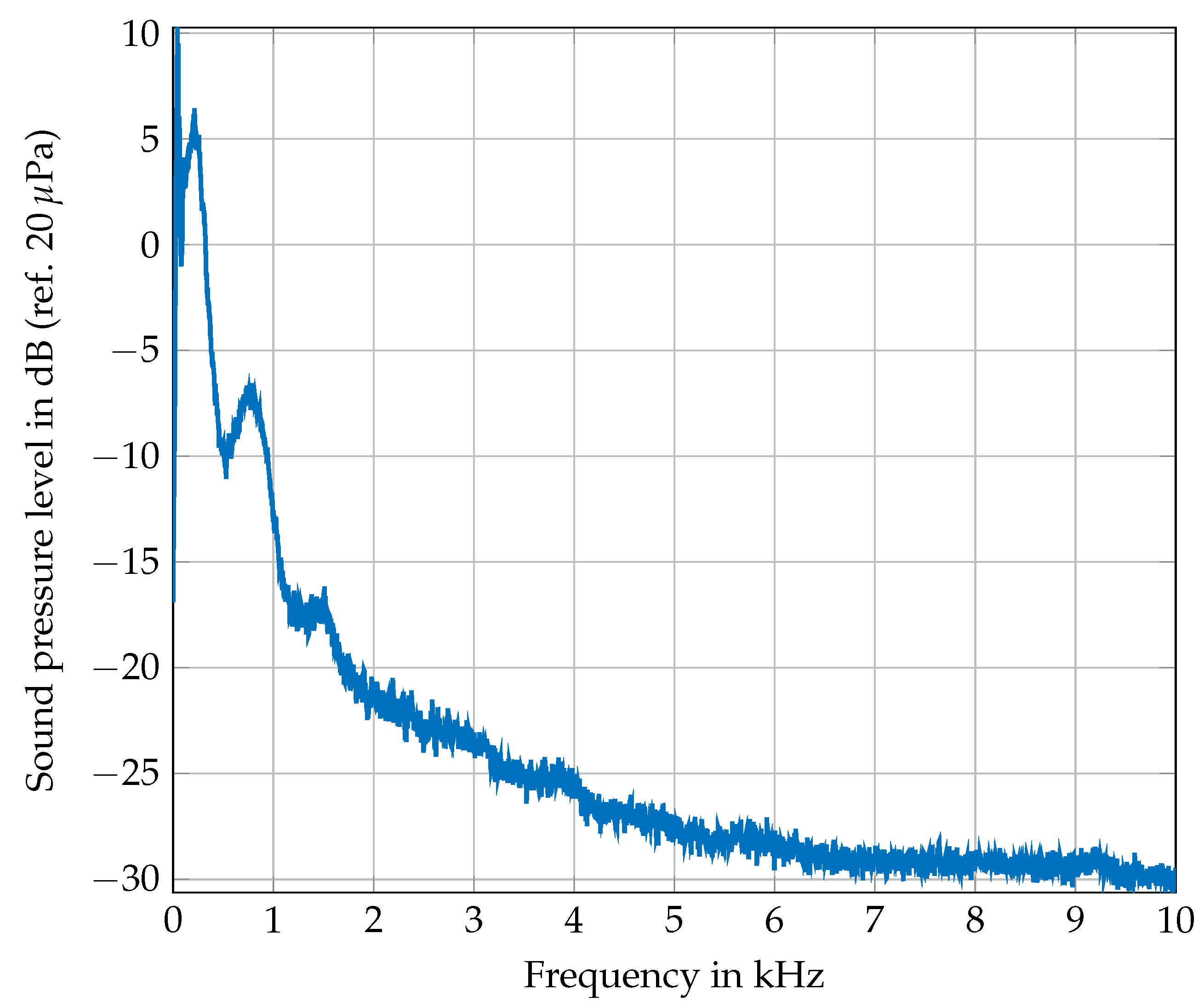
The recorded raw audio signals have to be pre-processed before they are suitable as inputs for a CNN. The selected microphone has a frequency bandwidth of 20–20,000 Hz. Even in a semi-anechoic room, like the ATB, external low frequency noise with several meters wavelength is measured. Sources of this noise are often construction sites or traffic on highways or airports. To eliminate these disturbances, all of the time signals are high-pass filtered by a butterworth filter of fourth order with a cut-off frequency of 40 Hz. Afterwards, the steps are visible in the time signal, like in Figure 1. Additionally, Figure 2 shows the spectrum of the signal from M13. It becomes apparent that the main frequency content is below 1 kHz. This holds for all of the measurements.
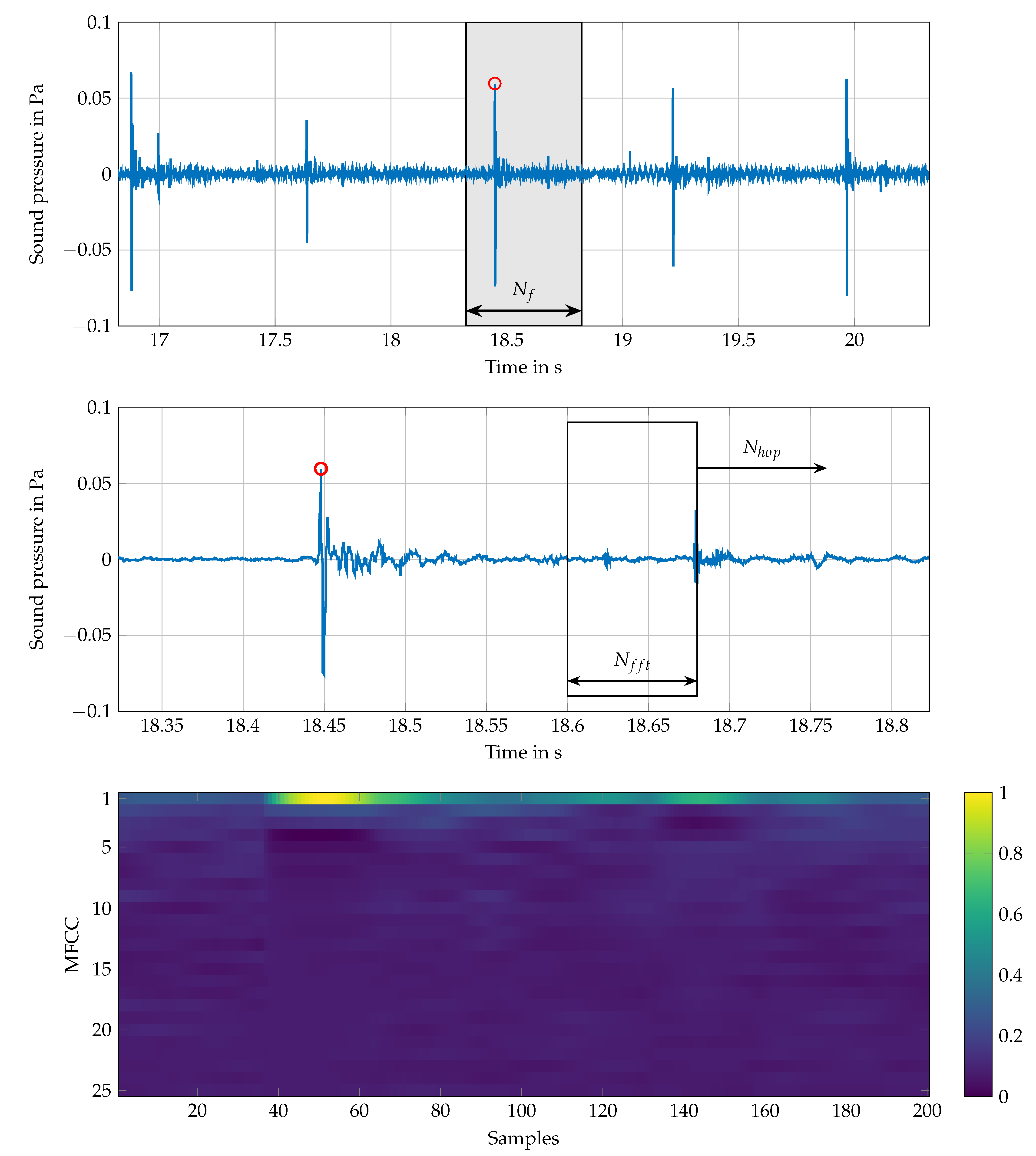
The objective of this work is to identify the subjects by their step sound. Therefore, the locations of single steps have to be determined in the time signal. The localization is performed with the find_peaks() method from SciPy (www.scipy.org/scipylib, accessed on 1 December 2020) library in Python. The peak to find is the heelstrike transient, since it is usually higher than the mid-stance peak. Two additional parameters are given to the find_peaks() method to ensure correct identification. First, the distance parameter is set to the number of samples that correspond to 500 ms, which is the lower bound for the step distance observed in all measurements. Second, the parameter height is set to five times the root mean square (RMS) value of the entire signal. This minimum height leads to a stable identification of the heelstrike transients while neglecting disturbance peaks or weak steps. Starting from the position of a heelstrike transient, a frame with samples is placed around it to separate the step, see Figure 3 (top). The heelstrike is placed at the first quarter of the frame. corresponds to the mean step duration of 500 ms. The frame time signal is normalized to a RMS value of 1 to ensure constant signal energy. The time signal is transformed into a spectrogram by means of a Fast Fourier Transform (FFT) with overlapping windows, see Figure 3 (mid). The size of the window is set to 4096 to achieve a frequency resolution of 12.5 Hz. Because the step sound peaks are rather short events with 5–10 ms duration, a time resolution of 2.5 ms is chosen for the spectrogram. This leads to a large overlapping of the windows and, thus, a small hop size of . The spectrogram is transformed to a mel-spectrogram by applying a mel filterbank [23]. The filterbank consists of 25 triangular shaped filters within the bandwidth from 0 to 1 kHz, since the main frequency content is located here, see Figure 2. The center frequencies are evenly distributed in the mel frequency domain. A discrete cosine transform (DCT) is applied to the result after calculating the logarithm of the mel-spectrogram.
As a result, each window in the frame is reduced to a vector of 25 so-called mel-frequency cepstral coefficients (MFCC). All 200 vectors of a frame are arranged in a matrix. This MFCC matrix is normalized to an interval of [0, 1]. Figure 3 (bottom) shows this matrix as a bitmap using a viridis colormap from Matplotlib (matplotlib.org, accessed on 1 December 2020).
Finally, 70 to 90 steps are identified in each measurement of Table 1. Each of these steps is transformed into a MFCC matrix and then exported as bitmap without compression. It serves as input to the CNN described in the following section.
4. Network
The pre-processing of the previous section transforms the walker identification problem into the domain of image classification tasks. In the last decade, powerful CNNs for image classification, like VGG16/19 [11], AlexNet [12], or DenseNet [13], emerged. Instances of these CNN with pre-trained weights are freely available within the Keras (keras.io) framework for example. The pre-trained networks can be used as a starting point, since they already learned to extract a large number of features from millions of pictures. By replacing the classification layers, new classes can be defined that are suitable for the desired application. The weights in the feature recognition layers are kept fixed, while the weights in the new layers are trained. This so-called transfer learning is well established and easy to implement. The number of parameters is the drawback of the pre-trained image classification networks, which easily exceeds several millions. In AlexNet, for example, only the convolutional layers contain nearly four million parameters.
4.1. Setup
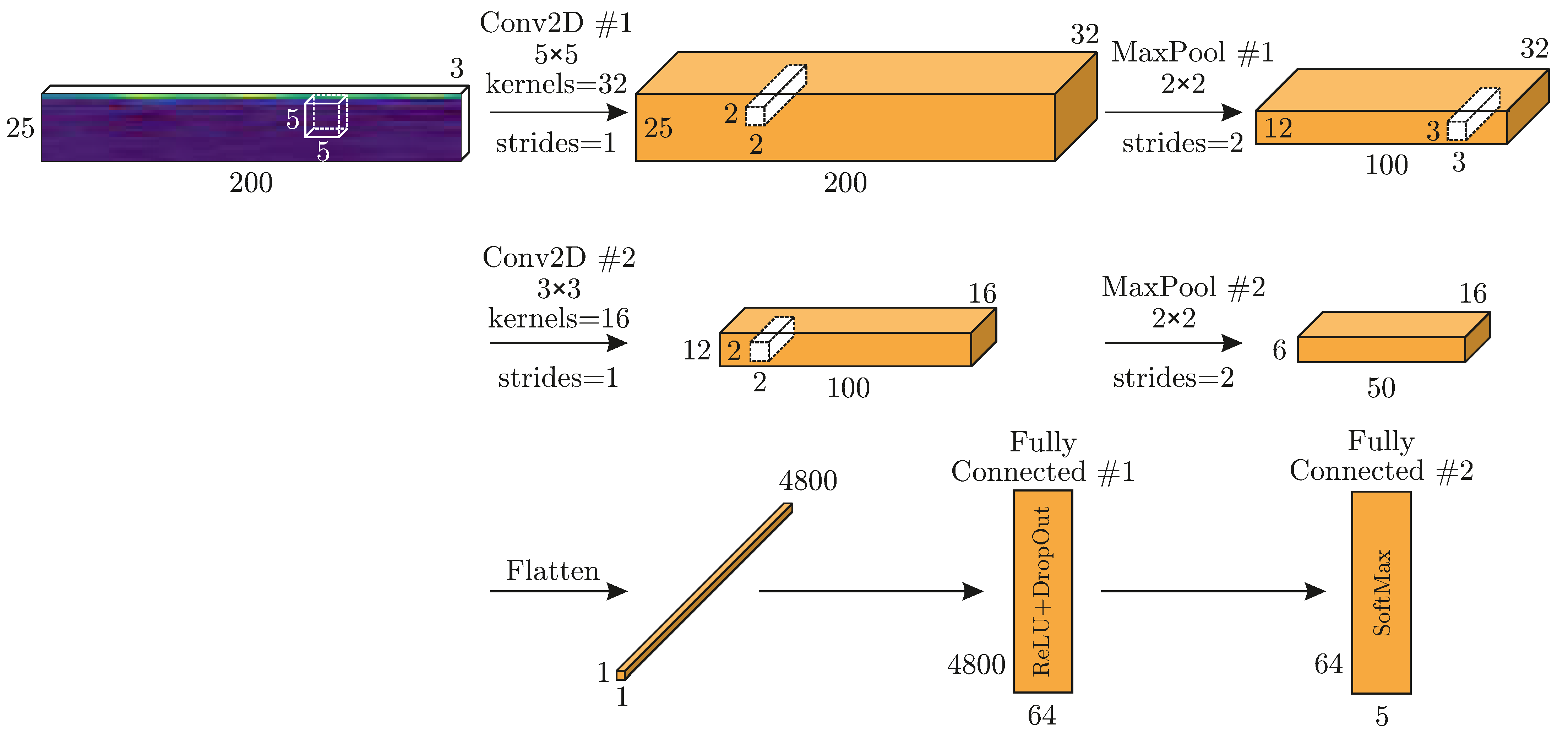
For this application, the objective is to generate a CNN that is computationally efficient and less demanding for computational power than AlexNet, etc., such that a future implementation on small computer architectures, like microcontrollers, is more feasible. Therefore, the network architecture that is shown in Figure 4 is set up. The input picture from the pre-processing with dimensions 25 × 200 × 3 (H × W × D) is convolved in two dimensions with 32 kernels of size 5 × 5. Because the strides parameter is set to one the result has size of 25 × 200 × 32. The spatial dimensions are reduced by factor two with a subsequent MaxPooling layer. After a second convolution with 16, 3 × 3 kernels, followed by a further MaxPooling layer, the result is a 6 × 50 × 16 tensor. After flattening, the data are fed through two fully connected (FC) layers. The last layer contains a SoftMax activation, which leads to five outputs that represent the probability of the corresponding class. The convolutional layers and the first FC layer use ReLu activation and are initialized according to [24]. Additionally, a DropOut is performed after each MaxPooling and the first FC layer. The principle structure is inherited from AlexNet. Several convolutional and MaxPooling layers are followed by a number of FC layers. Whenc ompared to the network architecture that is presented here, AlexNet consists of five convolutional and three FC layers, with a total of 61 million trainable parameters. Table 2 summarizes the number of trainable parameters for the network shown in Figure 4. With around three hundred thousand parameters, the net is much leaner than large image classification CNN and, therefore, easier to implement on small architectures with limited memory and computational capacity. The presented CNN is implemented within the Keras environment.
4.2. Training
The training of a CNN in Keras is straightforward. Besides several optimizers, different parameters and callback functions are available to steer the training and avoid overfitting. In the pre-processing, 1125 MFCC step bitmaps are generated. They are randomly split into train (75 %) and validation (25 %) datasets. Five different classes of subjects are defined representing the five outputs of the CNN. Table 3 shows the mapping of measurement and classes. A single class includes all of the measurements of a subject independent from walking direction or footwear.
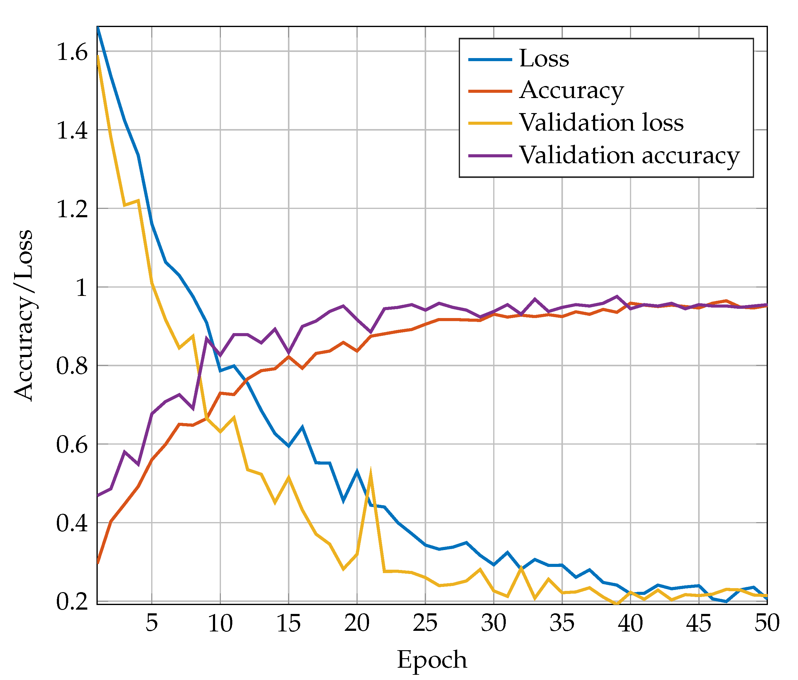
The training is carried out with the stochastic gradient descent (SGD) optimizer using a momentum of 0.9. The training spans over 50 epoches using a batch size of 16. A learning rate scheduler is used to ensure the convergence of the optimization process and avoid overfitting. Starting with a learning rate of it decreases linearly to in epoch 50. By the use of model checkpoints, the weights of the epoch with the best validation accuracy are saved during training. The training is executed on a Intel® Core™ i7-6820HQ CPU with 16 GB RAM and takes 6 s per epoch. Figure 5 shows a typical progress of accuracy and loss values over the training period. The training runs smoothly and no overfitting occurs. The learning rate scheduler and the DropOuts are adjusted properly. In this run, a maximum validation accuracy of 0.976 could be achieved.
5. Results
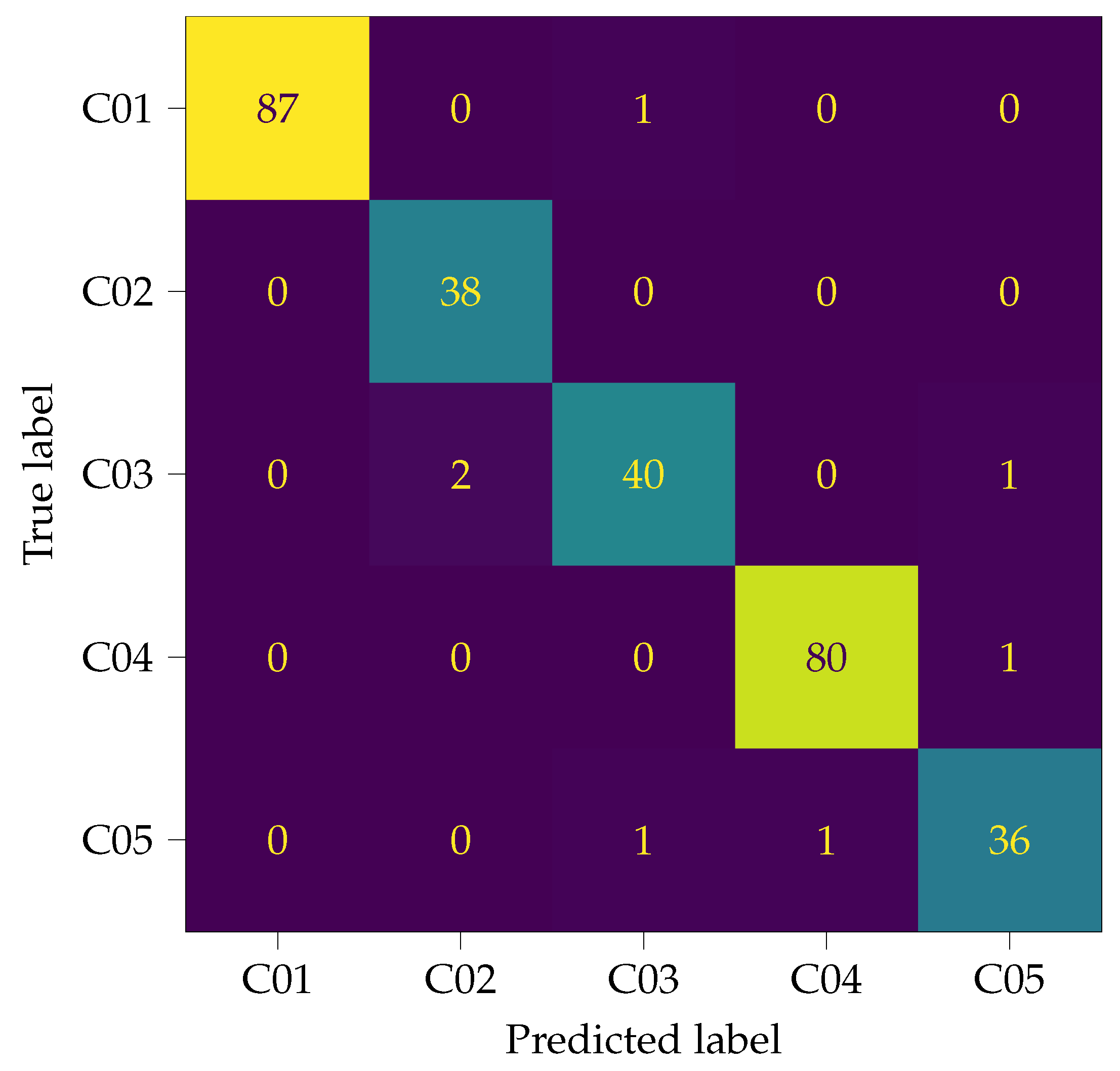
The CNN designed in the preceding section is evaluated against the entire validation dataset, which consists of 288 steps. Each step is classified by the CNN and then checked for correctness afterwards. The results are summarized in the confusion matrix shown in Figure 6. The majority of the classifications are correct. Only a few false detections are located in the upper and lower triangles of the matrix. Additional metrics are calculated to quantify the quality of the results. Therefore, the results are divided into true positive (step is labelled correctly), false positive (step is incorrectly labelled as belonging to class), and false negative (step belongs to class, but it is labelled incorrectly) predictions for each class. Based on these values, three metrics, precision P, recall R, and -score, which are widely used in machine learning, are calculated:
Table 4 summarizes the metrics for each class. The precision and recall metrics range between 0.93 and 1.0, while the -score is above 0.94 for all classes. The accuracy A, which is the ratio of correct predictions to all predictions, is 0.98 for this net. These results are excellent and, within this validation dataset, the CNN allows nearly perfect predictions. It is also noticeable that the classes C01 and C04 with the most steps gain the highest -score. When interpreting the metrics it has to be considered that these results represent the upper boundary of detection and cannot be reached in practical implementations. It has to be kept in mind that the recordings are conducted in a semi-anechoic room without any background noise and echoes. The detection of the steps in the time signals are clear, apart from some time shifts where the mid-stance peak is detected instead of the heelstrike transient. This is discussed in more depth in the following section.
Another topic shall be touched to conclude this section. The more superior the results of CNNs are, the less understandable and interpretable they are. CNNs are a kind of black box and the question “…why they predict what they predict…” [25] always arises when the results have to be interpreted. In the past years, several approaches were made to gain insight into CNNs and visualize which region in an image is relevant for prediction. In this paper, the Gradient-weighted Class Activation Mapping (Grad-CAM) approach [25,26] is applied to the CNN above. The Grad-CAM method produces a heatmap that is a kind of overlay to the original image. The heatmap highlights regions that lead to the prediction of the class. Grad-CAM uses the class specific gradients flowing into the last convolutional layer of the CNN to create it. No change or re-training of the CNN is necessary.
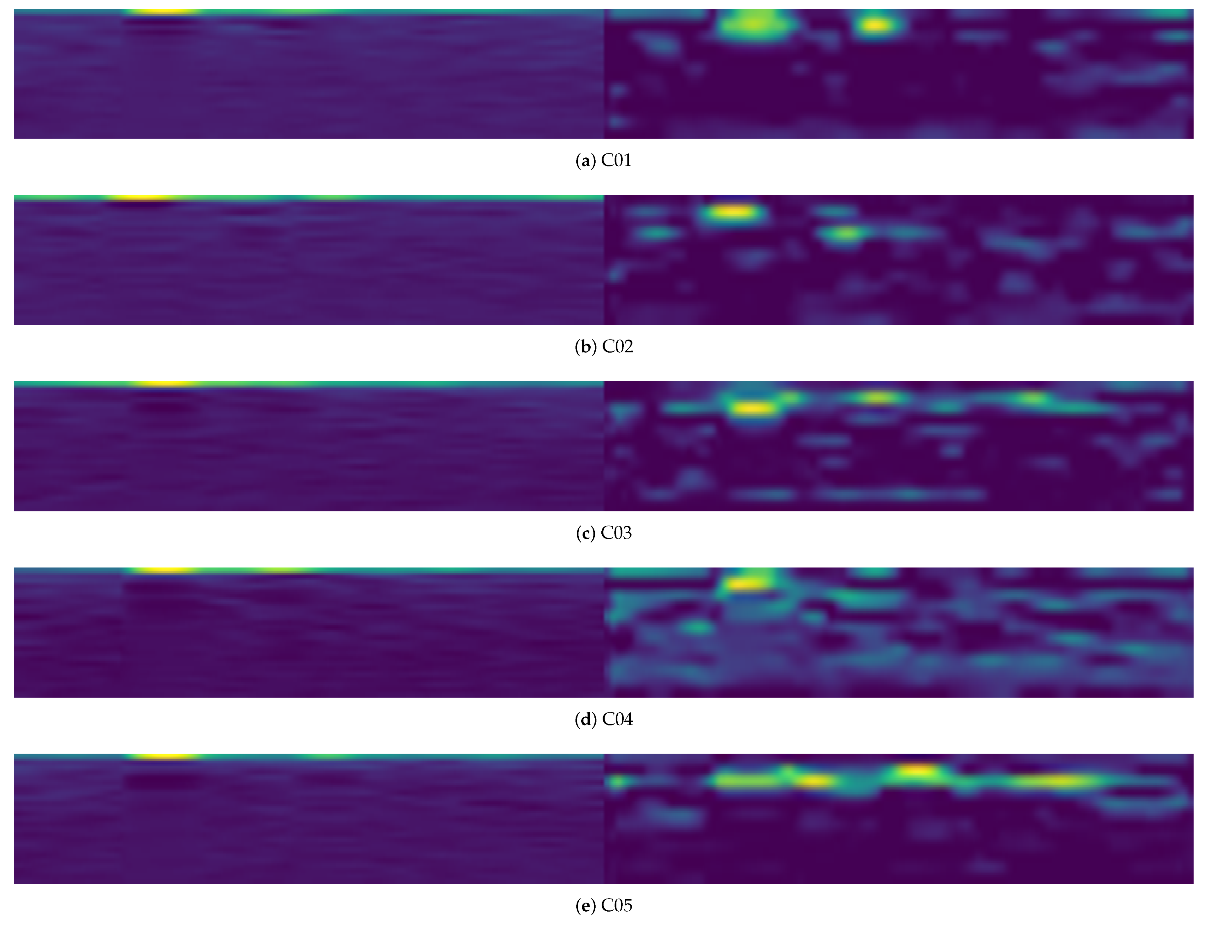
A heatmap is calculated for each of the 288 MFCC images of the validation dataset. The objective is to compare the heatmaps with the regions that the designer considers important. If there were differences, then the CNN would “look” everywhere but the step event. It would be a sign for a not properly trained net. In Figure 7a, a selected MFCC image for each class, together with the corresponding heatmap, are shown side-by-side. In all MFCC images, the location of the heelstrike transient is clearly identifiable in the first quarter, compare Figure 3 (bottom). A closer look also reveals the mid-stance peak. Looking at the heatmaps on the right hand side, it becomes obvious that the highlighted regions are mapping to the acoustic events in the MFCC images. Because this behavior holds for nearly all heatmaps of the validation dataset, it is assumed that the classification of the CNN is based on the step acoustics and that the functionality is given. The Grad-CAM method cannot prove a safe operation of the CNN, but it is able to create confidence by gaining insight into internal processes.
6. Challenges in Practical Applications
The CNN designed above is trained and validated with acoustic data being recorded in an anechoic environment. To roll-out this design for practical applications, a lot of boundary conditions have to be considered. Human gait, for example, is influenced by the footwear, the mood, injuries, etc., or even by extra weight that is carried. Furthermore, the environmental influences cannot be neglected. Long reverberation times in a corridor with tile floor produce echoes and complicate classification just as ambient noise. Several subjects in the location of recording produce a mixture of step sounds, which are usually paired with conversation. Unknown subjects may lead to incorrect or not clear identification results. Two practical challenges are addressed in the following sections. The objective is to provide an insight into the opportunities and limitations of person identification using CNN.
6.1. Different Footwear
Many factors influence the step sound of a walker. The footwear of the walker is the one with the largest impact apart from injuries or similar. The individual walking behavior is heavily “filtered” by the footwear of the walker. For practical implementations, the question arises as to whether a CNN trained to a subject with footwear A is able to identify the same subject with footwear B.
In the measurements for this paper, subjects 1 and 4 were recorded with different footwear, see Table 1. This gives the opportunity to perhaps answer the question raised above within a different footwear test (DFT). For this purpose, the CNN is trained without M07, M08, M11, and M12, which represent the measurements of subjects 1 and 4 with a second set of footwear. Table 5 summarizes the mapping of classes and measurements for the training. All of the training parameters and settings of the CNN are kept fixed as in the preceding section. After 50 epochs, a maximum validation accuracy of 0.958 could be achieved, which is comparable to the one of the original CNN (0.976). Table 6 summarizes the validation metrics for the DFT. The validation dataset has a reduced size of 192 steps due to the missing measurements. The metrics only show small changes. The -score is again over 0.94 for all classes.
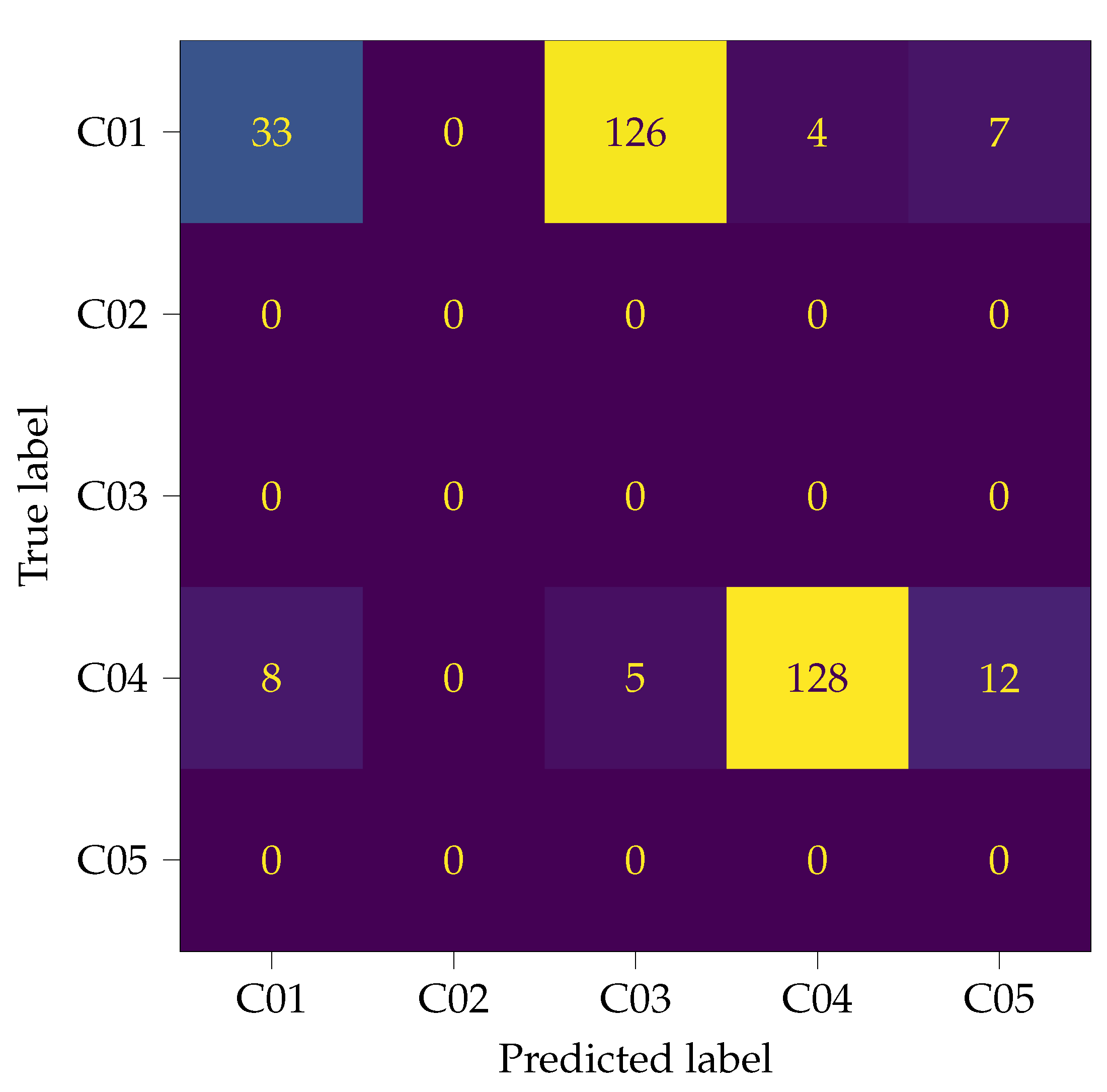
Because the measurements left out for training are not sub-divided into train and validation data, all 323 steps of M07, M08, M11, and M12 are given to the CNN for classification. The test results are summarized in the confusion matrix of Figure 8. The differences to the confusion matrix in Figure 6 become obvious. Subject 1 is misclassified in 137 of 170 cases. The prevailing majority is classified as subject 3, which suggests a strong similarity between C03 and M07/M08. In contrast to that, subject 4 is correctly classified in 128 of 153 cases. Table 7 shows the corresponding test metrics. The recall value drops, as expected, and leads to a poor -score, because of the misclassification of subject 1. The metrics for subject 4 are sufficient for classification.
From this test it can be concluded that the footwear has a strong impact on the classification results. The results for unknown footwear have to be considered with caution. As presented, it may work properly (e.g., subject 4), but it could also be completely misleading (e.g., for subject 1).
6.2. Influence of Noise
Footsteps are rather quiet sound events when compared to urban or indoor sound scenarios. Except for some high heel shoes, the footstep sounds are often masked by environmental noise and cannot be easily identified in practical measurement setups. Calculations with extra noise are conducted in this section to explore the potential of the CNN footstep detection.
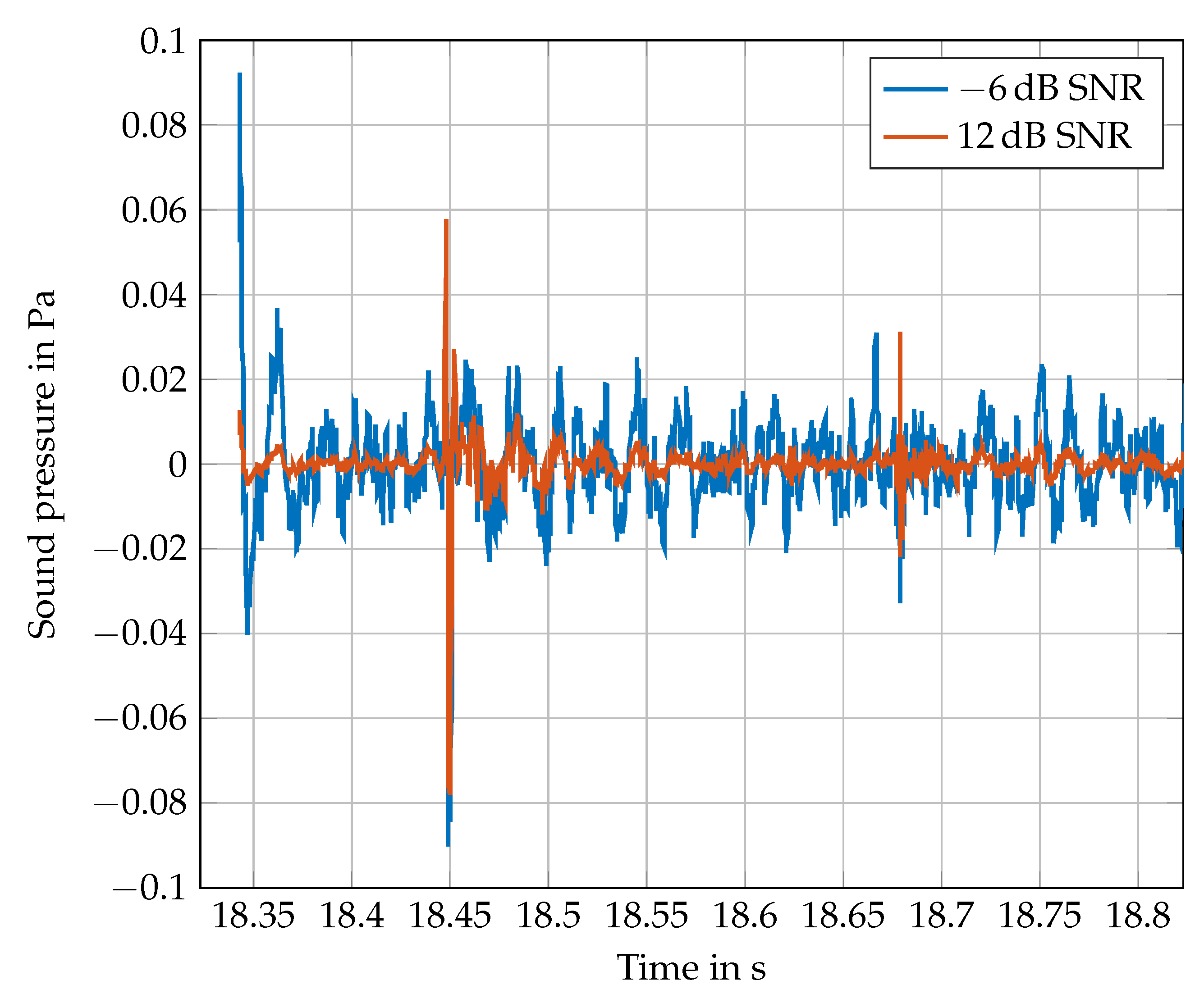
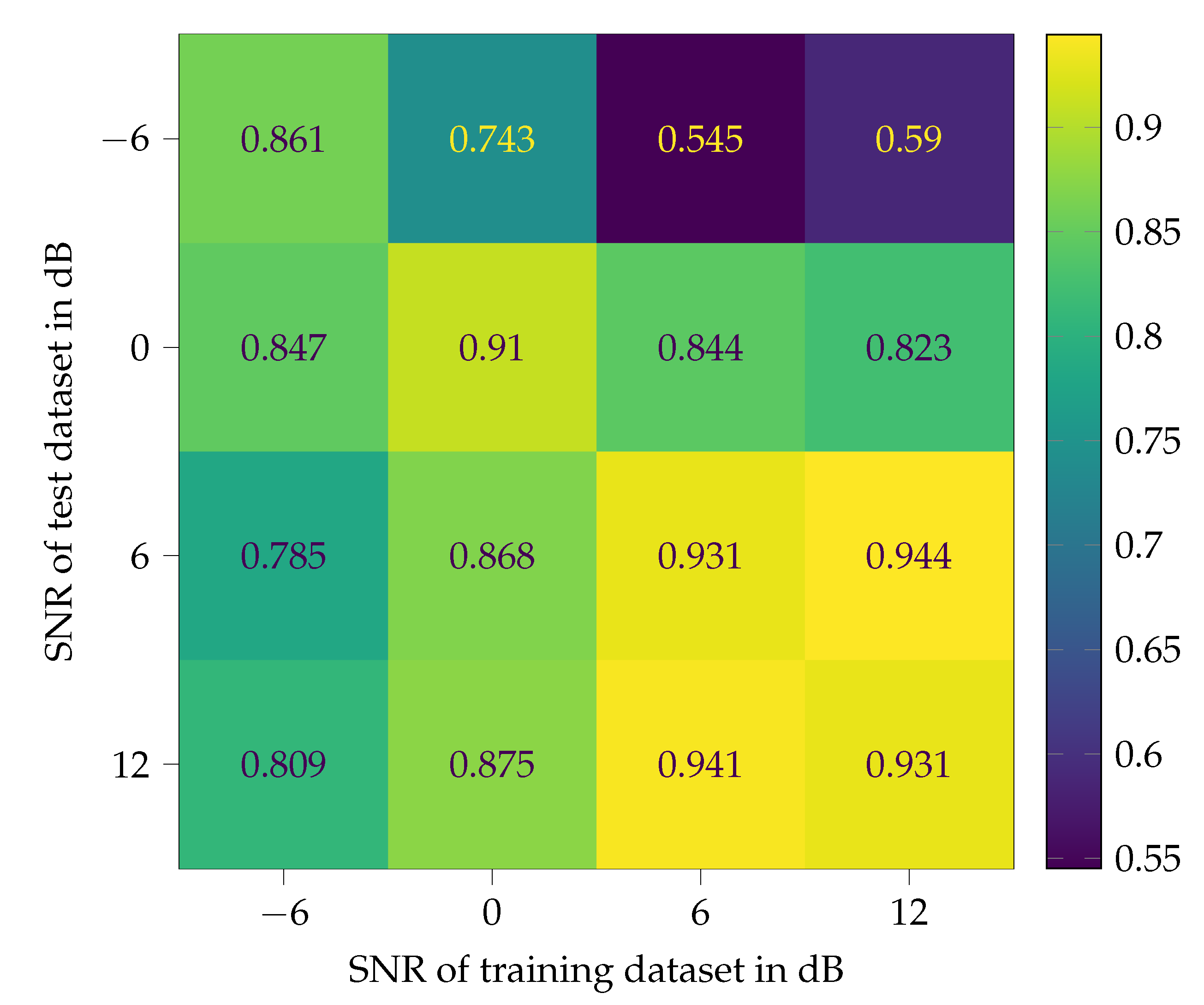
To explore the influence of noise in two ways, it is added to the training/validation data as well as to the test data. Four different signal-to-noise ratios (SNR) −6, 0, 6, and 12 dB are defined for this study. Therefore, the original footstep sounds measured in M01–M14 are treated as “pure” and noise free signals. The SNR only refers to the additional noise. In common measurement setups, SNR are much higher. These low values are selected to create representative conditions of environmental noise scenarios. Figure 9 shows an impression of the influence of different SNR on a signal. With a SNR of 12 dB, the footstep is clearly recognizable by eye, while, with −6 dB SNR, it is not. Nevertheless, the ear is able to detect the step in both time signals when played with a loudspeaker system. The CNN of Figure 4 is trained and tested with all SNR, which leads to a matrix of 16 tests. Pink or noise is chosen as additional noise, since its spectrum matches very well with that of the footstep sounds, compare Figure 2. Before the noise is added, it is high-pass filtered, like the original footstep sounds, see Section 3. A dataset for each SNR is created from all measurements. These datasets are split again into training (75 %) and validation (25 %) data. For each SNR, a CNN is trained with the corresponding train dataset. The validation data of a SNR serve as test data for the other SNR. The results are shown in confusion matrix style in Figure 10. The test accuracy is chosen for comparison of the different CNN. The validation accuracies of the CNN during training appear on the diagonal.
It becomes obvious that training and testing with a SNR of 6 dB and 12 dB lead to excellent classification results. The performance of the two CNN drop at a SNR of 0 dB and disappear at −6 dB. The CNN trained with 0 dB SNR is able to enhance the test accuracy up to 0.743 at −6 dB SNR, while the performance at 6 dB and 12 dB decreases significantly. Astonishing results can be achieved with the CNN that was trained with −6 dB SNR data. Although the validation accuracy is 0.861 only, test accuracies of around 0.8 are reached for all other datasets. It must be considered that the dataset with −6 dB SNR is really noisy, even for human ears.
The results of the test above can be summarized, as follows. If in the application phase of a CNN quiet and clear measurement are expected, training with additional noise in a mixing ratio of 12 dB and more would be sufficient and lead to stable classification results. When a significant presence of noise is expected, a SNR of 0 dB is recommended for the training data. A SNR of −6 dB should not be aimed at for practical applications. If it occurs, then it would not be acceptable and the entire setup should be redesigned. This case is only used in this paper to demonstrate the limits of feasibility.
The results are comparable to many problems in control applications. The robustness and performance are two opposing objectives that cannot be simultaneously maximized.
7. Conclusions & Outlook
The approach that is presented in this article is able to identify persons based on their step sound. It shows excellent performance with an accuracy of 0.98 and a minimum -score of 0.94 for all five classes. Only two convolutional and two fully connected layers with 314 k trainable parameters were needed to achieve the results. Furthermore, the confidence in the method was strengthened by the application of the Grad-CAM method. The depicted heatmaps revealed that the designed CNN uses areas of the MFCC bitmaps that are closely related to the step sound. Although the experiments were conducted in a laboratory environment, the results are promising that this method is capable of real world applications. To tackle challenges that may occur in practical applications, two of these, noise and different footwear, were addressed. The experimental data with different SNR were used for the training and test. When considering the low SNR values, the synthesized CNN showed astonishing performance. The influence of different footwear on the classification results showed the limitations of the CNN. One subject is identified with different shoes with a -score of 0.90, which is nearly perfect. The identification of the other subject failed, with a -score of 0.31. It can be concluded that, for correct classification, the CNN needs as many different footwear training samples as possible. Finally, it could be shown that image recognition CNN are able to solve problems in classifying complex audio signals.
Future work will transfer these results to comparable audio classification tasks. This paper is a pre-study for the further development of recognition applications in aerospace and traffic research.
Author Contributions
Conceptualization, methodology, software, validation, writing, S.A.; Investigation, experiments, S.A. and M.H. Both authors have read and agreed to the published version of the manuscript.
Funding
This research received no external funding.
Acknowledgments
The authors gratefully acknowledge the support of the individuals participating the acoustic lab tests.
Conflicts of Interest
The authors declare no conflict of interest.
Abbreviations
The following abbreviations are used in this manuscript:
| ATB | Acoustic transmission loss test facility |
| CNN | Convolutional neural network |
| CW | Clockwise |
| CCW | Counter-clockwise |
| DCASE | Detection and Classification of Acoustic Scenes and Events |
| DCT | Discrete cosine transform |
| DFT | Different footwear test |
| DLR | German Aerospace Center |
| FC | Fully connected |
| FFT | Fast Fourier transform |
| MFCC | Mel-frequency cepstral coefficients |
| MTP | Metatarso-phalangeal |
| RMS | Root mean square |
| SGD | Stochastic gradient descent |
| SNR | Signal-to-noise ratio |
| SPL | Sound pressure level |
References
- Whittle, M.W. Gait Analysis—An Introduction, 4th ed.; Elsevier: Amsterdam, The Netherlands, 2007. [Google Scholar]
- Nixon, M.S.; Chellappa, R.; Tan, T. Human Identification Based on Gait; International Series on Biometrics; Springer: Berlin, Germany, 2006; Volume 4. [Google Scholar] [CrossRef]
- Makela, K.; Hakulinen, J.; Turunen, M. The use of walking sounds in supporting awareness. In Proceedings of the 2003 International Conference on Auditory Display, Boston, MA, USA, 6–9 July 2003; pp. 144–147. [Google Scholar]
- Altaf, M.U.B.; Butko, T.; Juang, B.H.F. Acoustic Gaits: Gait Analysis With Footstep Sounds. IEEE Trans. Biomed. Eng. 2015, 62, 2001–2011. [Google Scholar] [CrossRef] [PubMed]
- Wang, C.; Wang, X.; Long, Z.; Yuan, J.; Qian, Y.; Li, J. Estimation of Temporal Gait Parameters Using a Wearable Microphone-Sensor-Based System. Sensors 2016, 16, 2167. [Google Scholar] [CrossRef] [PubMed]
- Alpert, D.T.; Allen, M. Acoustic gait recognition on a staircase. In Proceedings of the World Automation Congress (WAC), Kobe, Japan, 19–23 September 2010. [Google Scholar]
- Diapoulis, G.; Rosas, C.; Larsson, K.; Kropp, W. Person identification from walking sound on wooden floor. In Proceedings of the Euronoise 2018, Heraklion, Greece, 27–31 May 2018; pp. 1727–1732. [Google Scholar]
- Geiger, J.T.; Kneißl, M.; Schuller, B.W.; Rigoll, G. Acoustic Gait-based Person Identification using Hidden Markov Models. In Proceedings of the 2014 Workshop on Mapping Personality Traits Challenge and Workshop, Istanbul, Turkey, 12 November 2014; Gunes, H., Ed.; ACM: New York, NY, USA, 2014; pp. 25–30. [Google Scholar] [CrossRef] [Green Version]
- Huang, J.; Di Troia, F.; Stamp, M. Acoustic Gait Analysis using Support Vector Machines. In Proceedings of the 4th International Conference on Information Systems Security and Privacy (ICISSP), Funchal, Portugal, 22–24 January 2018; SCITEPRESS—Science and Technology Publications: Setúbal, Portugal, 2018; pp. 545–552. [Google Scholar] [CrossRef]
- Pan, S.; Wang, N.; Qian, Y.; Velibeyoglu, I.; Noh, H. Indoor Person Identification through Footstep Induced Structural Vibration. In Proceedings of the 16th International Workshop on Mobile Computing Systems and Applications, Santa Fe, NM, USA, 12–13 February 2015; Association for Computing Machinery: New York, NY, USA, 2015. [Google Scholar] [CrossRef]
- Simonyan, K.; Zisserman, A. Very Deep Convolutional Networks for Large-Scale Image Recognition. In Proceedings of the Third International Conference on Learning Representations (ICLR), San Diego, CA, USA, 7–9 May 2015; Bengio, Y., Lecun, Y., Eds.; 2015. [Google Scholar]
- Krizhevsky, A.; Sutskever, I.; Hinton, G.E. ImageNet Classification with Deep Convolutional Neural Networks. Commun. ACM 2017, 60, 84–90. [Google Scholar] [CrossRef]
- Huang, G.; Liu, Z.; van der Maaten, L.; Weinberger, K.Q. Densely Connected Convolutional Networks. In Proceedings of the IEEE Conference on Computer Vision and Pattern Recognition (CVPR), Honolulu, HI, USA, 21–26 July 2017. [Google Scholar]
- Lasseck, M. Bird Song Classification in Field Recordings: Winning Solution for NIPS4B 2013 Competition. In Proceedings of the Neural Information Processing Scaled for Bioacoustics (NIPS4B), Lake Tahoe, NV, USA, 10 December 2013; pp. 176–181. [Google Scholar]
- Sprengel, E.; Jaggi, M.; Kilcher, Y.; Hofmann, T. Audio Based Bird Species Identification Using Deep Learning Techniques. In Proceedings of the Working Notes of CLEF 2016, Évora, Portugal, 5–8 September 2016; CEUR Workshop Proceedings: Aachen, Germany, 2016; pp. 547–559. [Google Scholar]
- Zhao, X.; Wang, D. Analyzing noise robustness of MFCC and GFCC features in speaker identification. In Proceedings of the IEEE International Conference on Acoustics, Speech and Signal Processing, Vancouver, BC, Canada, 26–31 May 2013; pp. 7204–7208. [Google Scholar]
- Lane, N.D.; Georgiev, P.; Qendro, L. DeepEar: Robust Smartphone Audio Sensing in Unconstrained Acoustic Environments using Deep Learning. In Proceedings of the 2015 ACM International Joint Conference on Pervasive and Ubiquitous Computing—UbiComp’15, Osaka, Japan, 7–11 September 2015; Mase, K., Langheinrich, M., Gatica-Perez, D., Gellersen, H., Choudhury, T., Yatani, K., Eds.; ACM Press: New York, NY, USA, 2015; pp. 283–294. [Google Scholar] [CrossRef] [Green Version]
- Cummins, N.; Amiriparian, S.; Hagerer, G.; Batliner, A.; Steidl, S.; Schuller, B.W. An Image-based Deep Spectrum Feature Representation for the Recognition of Emotional Speech. In Proceedings of the 25th ACM international conference on Multimedia, Mountain View, CA, USA, 23–27 October 2017; Liu, Q., Lienhart, R., Wang, H., Chen, S.W.T., Boll, S., Chen, P., Friedland, G., Li, J., Yan, S., Eds.; ACM: New York, NY, USA, 2017; pp. 478–484. [Google Scholar] [CrossRef]
- Dai, W.; Li, J.; Pham, P.; Das, S.; Qu, S. Acoustic Scene Recognition with Deep Neural Networks. In Proceedings of the Detection and Classification of Acoustic Scenes and Events (DCASE), Budapest, Hungary, 3 September 2016. [Google Scholar]
- Kahl, S.; Hussein, H.; Fabian, E.; Schloßhauer, J.; Thangaraju, E.; Kowerko, D.; Eibl, M. Acoustic Event Classification Using Convolutional Neural Networks. In Proceedings of the INFORMATIK 2017, Chemnitz, Germany, 25–29 September 2017; pp. 2177–2188. [Google Scholar]
- Lim, H.; Park, J.; Kyogu, L.; Han, Y. Rare sound event detection using 1D convolutional recurrent neural networks. In Proceedings of the Detection and Classification of Acoustic Scenes and Events (DCASE), Munich, Germany, 16–17 November 2017. [Google Scholar]
- Sakashita, Y.; Aono, M. Acoustic Scene Classification by Ensemble of Spectrograms Based on Adaptive Temporal Divisions. In Proceedings of the Detection and Classification of Acoustic Scenes and Events (DCASE), Surrey, UK, 19–20 November 2018. [Google Scholar]
- Davis, S.; Mermelstein, P. Comparison of parametric representations for monosyllabic word recognition in continuously spoken sentences. IEEE Trans. Acoust. Speech Signal Process. 1980, 28, 357–366. [Google Scholar] [CrossRef] [Green Version]
- He, K.; Zhang, X.; Ren, S.; Sun, J. Delving Deep into Rectifiers: Surpassing Human-Level Performance on ImageNet Classification. In Proceedings of the IEEE International Conference on Computer Vision (ICCV), Santiago, Chile, 7–13 December 2015; pp. 1026–1034. [Google Scholar]
- Selvaraju, R.R.; Cogswell, M.; Das, A.; Vedantam, R.; Parikh, D.; Batra, D. Grad-CAM: Visual Explanations From Deep Networks via Gradient-Based Localization. In Proceedings of the IEEE International Conference on Computer Vision (ICCV), Venice, Italy, 22–29 October 2017. [Google Scholar]
- Chollet, F. Deep Learning with Python; Manning Publications Company: Shelter Island, NY, USA, 2018. [Google Scholar]
Figure 1.
Time signal with seven steps taken from M13; magnification: single step.

Figure 2.
Spectrum of time signal from M13.

Figure 3.
Step pre-processing with data from M13; (top) time signal with marked heelstrike transient and surrounding frame; (middle) single step with sliding window; and, (bottom) MFCC image of frame.
Figure 3.
Step pre-processing with data from M13; (top) time signal with marked heelstrike transient and surrounding frame; (middle) single step with sliding window; and, (bottom) MFCC image of frame.

Figure 4.
CNN architecture.

Figure 5.
Progress of accuracy and loss.

Figure 6.
Confusion matrix.

Figure 7.
CNN at work, same colorbar as in Figure 3; left: MFCC image, right: Grad-CAM heatmap.
Figure 7.
CNN at work, same colorbar as in Figure 3; left: MFCC image, right: Grad-CAM heatmap.

Figure 8.
Confusion matrix of the DFT.

Figure 9.
Single step time signal, see Figure 3, with additional noise.
Figure 9.
Single step time signal, see Figure 3, with additional noise.

Figure 10.
Test accuracy of classification.


Table 1.
Summary of measurements.
| Measurement | Subject (Gender) | Direction | Footwear | Measurement | Subject (Gender) | Direction | Footwear |
|---|---|---|---|---|---|---|---|
| M01 | 1 (m) | CW | A | M08 | 1 (m) | CCW | D |
| M02 | 1 (m) | CCW | A | M09 | 4 (m) | CW | E |
| M03 | 2 (m) | CW | B | M10 | 4 (m) | CCW | E |
| M04 | 2 (m) | CCW | B | M11 | 4 (m) | CW | F |
| M05 | 3 (m) | CW | C | M12 | 4 (m) | CCW | F |
| M06 | 3 (m) | CCW | C | M13 | 5 (fm) | CW | G |
| M07 | 1 (m) | CW | D | M14 | 5 (fm) | CCW | G |
Table 2.
Trainable layer parameters.
| Layer | No. Trainable Parameters | ||
|---|---|---|---|
| Conv2D #1 | = | 2432 | |
| Conv2D #2 | = | 4624 | |
| FC #1 | 4800 | = | 307,264 |
| FC #2 | = | 325 | |
| Total | 314,645 | ||
Table 3.
Mapping of classes and measurements.
| Class | Measurements |
|---|---|
| C01 | M01, M02, M07, M08 |
| C02 | M03, M04 |
| C03 | M05, M06 |
| C04 | M09, M10, M11, M12 |
| C05 | M13, M14 |
Table 4.
Validation metrics.
| Class | Precision | Recall | -Score | No. Steps |
|---|---|---|---|---|
| C01 | 1.00 | 0.99 | 0.99 | 88 |
| C02 | 0.95 | 1.00 | 0.97 | 38 |
| C03 | 0.95 | 0.93 | 0.94 | 43 |
| C04 | 0.99 | 0.99 | 0.99 | 81 |
| C05 | 0.95 | 0.95 | 0.95 | 38 |
Table 5.
Mapping of classes and measurements for the DFT.
| Class | Measurements |
|---|---|
| C01 | M01, M02 |
| C02 | M03, M04 |
| C03 | M05, M06 |
| C04 | M09, M10 |
| C05 | M13, M14 |
Table 6.
Validation metrics of the DFT.
| Class | Precision | Recall | -Score | No. Steps |
|---|---|---|---|---|
| C01 | 0.95 | 0.93 | 0.94 | 44 |
| C02 | 0.93 | 0.97 | 0.95 | 38 |
| C03 | 0.95 | 0.98 | 0.97 | 43 |
| C04 | 0.98 | 0.95 | 0.96 | 42 |
| C05 | 1.00 | 0.96 | 0.98 | 25 |
Table 7.
Test metrics of the DFT.
| Class | Precision | Recall | -Score | No. Steps |
|---|---|---|---|---|
| C01 | 0.80 | 0.19 | 0.31 | 170 |
| C04 | 0.97 | 0.84 | 0.90 | 153 |
Publisher’s Note: MDPI stays neutral with regard to jurisdictional claims in published maps and institutional affiliations. |
© 2021 by the authors. Licensee MDPI, Basel, Switzerland. This article is an open access article distributed under the terms and conditions of the Creative Commons Attribution (CC BY) license (https://creativecommons.org/licenses/by/4.0/).
Share and Cite
MDPI and ACS Style
Algermissen, S.; Hörnlein, M. Person Identification by Footstep Sound Using Convolutional Neural Networks. Appl. Mech. 2021, 2, 257-273. https://0-doi-org.brum.beds.ac.uk/10.3390/applmech2020016
AMA Style
Algermissen S, Hörnlein M. Person Identification by Footstep Sound Using Convolutional Neural Networks. Applied Mechanics. 2021; 2(2):257-273. https://0-doi-org.brum.beds.ac.uk/10.3390/applmech2020016
Chicago/Turabian StyleAlgermissen, Stephan, and Max Hörnlein. 2021. "Person Identification by Footstep Sound Using Convolutional Neural Networks" Applied Mechanics 2, no. 2: 257-273. https://0-doi-org.brum.beds.ac.uk/10.3390/applmech2020016