New Numerical and Measurements Flow Analyses Near Radars

Abstract

An experimental and numerical investigation of the flow near a blunt body has been conducted in this study. Most experimental methods of flow studies use flow visualization and probes introduction into the flow field. The main goal of this research was the development of a new methodology to analyze flows, and to measure flow characteristics without taking into account the distorting effects of measuring probes. A series of experiments were performed on a ground surveillance radar in the Price-Païdoussis subsonic wind tunnel. Forces and moments were measured as functions of wind speeds and angular positions by the use of a six-component aerodynamic scale. A Computational Fluid Dynamics three-dimensional model was employed to analyze the wake region of the ground surveillance radar. A turbulence reduction system was proposed and analyzed in this research. The use of the proposed turbulence reduction system was found to be an effective way to reduce turbulent flow intensity by 50%, drag coefficients by 9.6%, and delay the flow transition point by 7.6 times.

1. Introduction

Blunt body flow analyses are very important in Engineering. Most bodies and structures do not present a streamlined shape; for this reason, an accurate analysis of wake regions would lead to a major understanding of turbulence flows and turbulence reduction mechanisms [1]. Blunt bodies in turbulent flow conditions can lead to material fatigue and damage, and therefore, to increased drag and energy consumption. There are few studies, both in theoretical and in experimental research related to methods of studying flow behaviors in the presence of blunt bodies [2,3]. A methodology to measure and analyze the flow characteristics near a full-size “Ground Surveillance Radar” without introducing probes into the flow field, that would affect its structure, to the best of our knowledge, has not been described in the literature. The proposed methodology employs a quantitative approach [4] to analyze the wake region to evaluate the turbulence intensity, drag coefficient, pressure distribution coefficient, and boundary separation of a flow near a blunt body. A procedure to quantitatively validate numerical models using experimental data from wind tunnel tests, including an analysis of a proposed “turbulence reduction system” is also part of this research.

The experimental tests were performed for the ground surveillance radar in the Price-Païdoussis subsonic wind tunnel at our Research Laboratory in Active Controls, Avionics and Aeroservoelasticity LARCASE. The LARCASE laboratory is one of the few multidisciplinary aerospace research laboratories in Canada that has four pieces of state-of-the-art research equipment, such as a Cessna Citation X Business Aircraft Research Flight Simulator, a Bombardier series regional jet CRJ-700 Research Flight Simulator, an Autonomous Aerial System UAS-S4 from Hydra Technologies and a Subsonic Wind Tunnel Price-Païdoussis. At the LARCASE, new methodologies in the aeronautical industry have been developed in the areas of actuated morphing wings and wing-tip systems [5,6,7], upper surface optimization of wing shapes for unmanned aerial systems [8,9,10,11], and Computational Fluid Dynamics models validations with experimental results from subsonic wind tunnel tests [12,13].

2. Literature Review

2.1. Wake Characteristics of Blunt Bodies

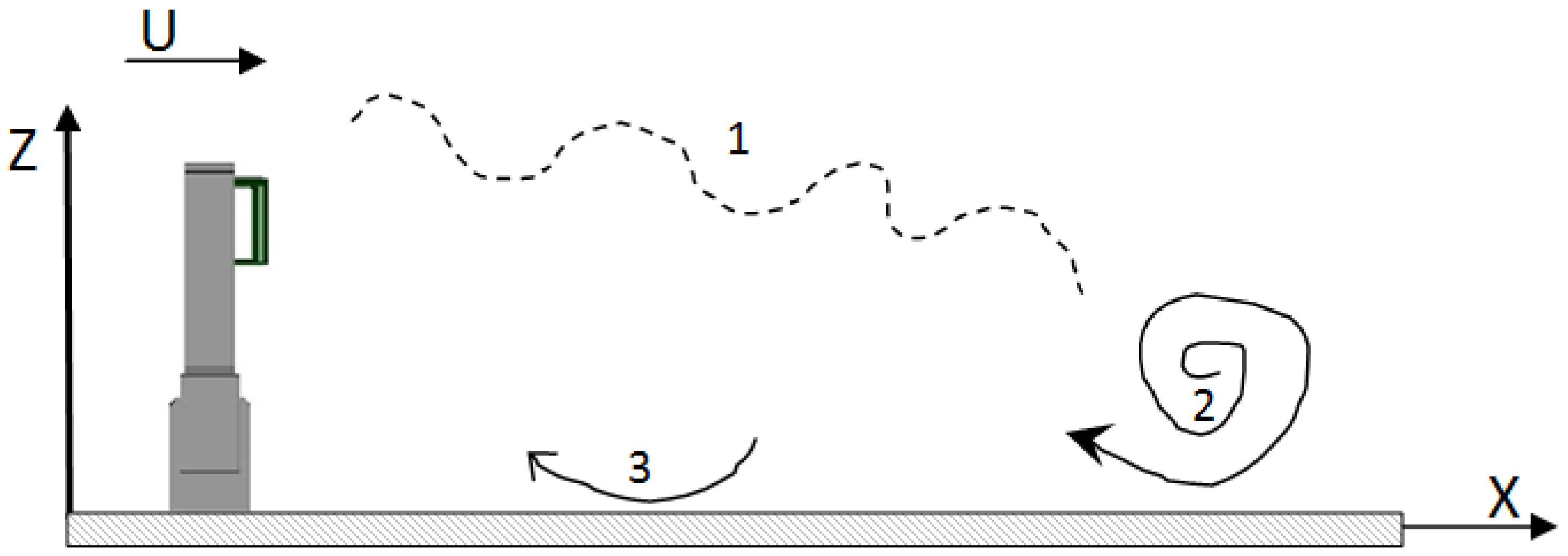
The boundary layer at the blunt body surface can be described in terms of flow separation, shear layers, vortex shedding, flow recirculation, and vortex formation, which may lead to a high surface drag coefficient. The reason is that the sharp edges of blunt bodies accelerate a transition to turbulent flow and a flow separation dominated by vortices and eddies [14,15]. The “ground surveillance radar” in this study had the same characteristics as a blunt body while the wake region had a turbulent flow behavior. The “ground surveillance radar” will be shortened by “radar” in the following sections. Figure 1 illustrates the flow behavior at the wake on a blunt body (radar), as explained in experimental research papers done on blunt bodies. On the left side of Figure 1, the radar model is visualized, while on its right side, the flow starts to separate, and then reattach on the radar upper surface, but the viscous forces and shear layers are not strong enough [16,17]. The detached shear layer path was indicated by number 1. At the wake region, a closed boundary would form; the length and width increase as the recirculation regions indicated by number 2, and the separation regions indicated by number 3 grow at the rear of the blunt body.

2.2. Turbulence Model

Most common flows encountered in nature and industrial applications are three-dimensional, and they are turbulent. There are the Reynolds-Averaged Navier-Stokes (RANS) one-equation turbulence models, such as the Spalart-Allmaras model, that are useful in wings and wing tip CFD simulations [18], and two-equation models such as k-ε models and k-ω models. In the next section, only the k-ε turbulence model will be used. The k-ε turbulence model predicts the flow behavior by solving the RANS equations where k is the turbulence kinetic energy and ε represents the rate of dissipation of turbulence kinetic energy; it is also a suitable model for solving external flow problems with complex geometries where the wall function and y⁺ values have to be carefully considered for each type of simulation [19,20]. Solving at the flow smallest scales, near the wall region, as well as at the flow largest scales, has led to the development of hybrid models, which combine the best properties of RANS with those of Large Eddie Simulation (LES). One of these hybrid techniques is the Detached Eddy Simulation (DES) model, where the regions close to the walls are solved using a RANS model, while the rest of the flow is solved with an LES approach [21,22].

The choice of a hybrid model was the best option to solve the flow model of the radar in this paper, because of the fact that important pressure gradients, eddies, and vortices were expected.

2.3. Model Validation

According to the ASME’s guide [23], uncertainties should be taken into account during the validation process of a numerical model. To validate a model, a specific metric is not imposed by ASME, but this metric should “be equal to zero” when the data is identical to the experimental results.

The “Area Metric” method allows the comparison of simulation results with experimental data. Moreover, this metric meets all the ASME’s requirements including the uncertainties modeling. This method has an important advantage with respect to classical methods for being able to evaluate and subsequently refuse or accept the proposed model [24,25]. This method is robust, as it provides quantitative measures of differences between the predicted and experimental data, and enables a graphical representation of these differences in the same physical units as for experimental data [26,27]. The measurement of the error d(P,O) is evaluated using Equation (1) on the entire range of the distributed data, where P(x) are the predicted values and O(X) are the observed values obtained during wind tunnel tests. This method is applied using the Cumulative Distribution Function (CDF) of experimental and numerical model data. Both CDFs are step functions and the variable A represents the difference between the model and the experimental test data.

$$A=d\left(P,O\right)={{\displaystyle \int }}_{-\infty }^{\infty }\left|P\left(x\right)-O\left(x\right)\right| dx$$

(1)

2.4. Vortex Detection

A vortex detection technique would greatly improve the results obtained in our research. There are a few vortex techniques developed in the last years, but the classical and more used vortex techniques are Q-criterion, Delta-criterion, and Lambda2-criterion [28]. The vortex detection technique lambda2 (suggested by the reviewers) is used mainly for body shapes where multiples vortices are presented. The radar body is a symmetric blunt body with one main vortex created by the boundary layer at its upper surface. We have consulted the suggested articles, as well as other articles in which various vortex techniques were used, and we found that the Q-criterion applies to the shape of the radar, and to the subsonic flow velocity in this study, and is less time consuming than the lambda2 criterion.

Largely steady or recirculation vortices at the wake region can orientate the flow in different directions and change the pressure distribution around the blunt body surface. Unsteady vortices can store energy and dissipate it in the wake flow, thus increasing the induced drag of the blunt body. Besides using the flow variables, such as velocity, pressure, and vorticity, it is challenging to analyze vortices at the surface and the wake region of a blunt body. From the classical vortex detection techniques [28,29] studied in the literature, the Q-Criterion [30] was found to be well suited to accurately identify vortex location, strength, and behavior in the flow field encountered in the radars wake region. The Q-Criterion vortex representation technique shows the variation of the rotational and deformation components of a fluid element in the flow field.

Equation (2) was programmed in the CFD model, in which Ω is the vorticity magnitude and S is the rate of strain.

$$Q=\frac{1}{2}\left(W^2-S^2\right)$$

(2)

The vortex detection technique Q-Criterion shows the local balance between the shear strain rate and the rotation rate or vorticity magnitude near the wake region of the radar. The Q-Criterion allows separating the region of the location where the strength of rotation overcomes the strain rate of a flow field. The threshold applied to the Q-Criterion plays an important role in detecting the outer shell of the vortex, as well as the strength of the vortices. The threshold values for Q-Criterion 10¹ < Q ≤ 10⁶ were chosen to account for the highest velocity of the flow inside the wind tunnel (15 m/s), the large size of the radar, and the fully turbulent flow at the wake region.

The vortices made up sheering motion, as well as their inviscid part cannot be captured using the Q-criterion. Most of the classical vortex detection techniques are limited to the narrow core region of vortices and are not applied outside it. Classical vortex criteria are tools to capture the topological structures of the flow rather than to extract and quantify values of individual vortices [31,32]. We are presenting results obtained using the Q-criterion for the original radar without a turbulence reduction system and for the radar with a turbulence reduction system.

2.5. Wind Tunnel

There are two main factors to be considered in a wind tunnel test procedure for blunt bodies; the “blockage constraint” of a closed test section and the Reynolds number. Different techniques and methods were established to measure, and thus to reduce the impact of blockage constraint on experimental data. It was found that the blockage area ratio should be 10% to remove wall interference and to calculate the wind tunnel empirical factor ω needed to remove the blockage constraint from aerodynamic coefficients. The Reynolds number plays an important role in experimental testing because of the fact that flow separation and turbulence are often dependent on the Reynolds number [33].

3. Research Objectives

The research objectives are:

(1)

The design of a new methodology for numerical and experimental analysis of turbulent flows.

(2)

The quantitative metrics consideration to measure flow analysis improvements.

(3)

The analysis of a “turbulence reduction system” for blunt bodies.

4. Apparatus and Instrumentation

The Applied Research Laboratory in Active Controls, Avionics, and Aeroservoelasticity LARCASE team obtained the Subsonic Wind Tunnel Price-Païdoussis for numerical model validation and testing in the Aerospace field. The details of this Blow-Down Subsonic Wind Tunnel, the aerodynamic scale, as well as the instrumentation used in this research are described in this section.

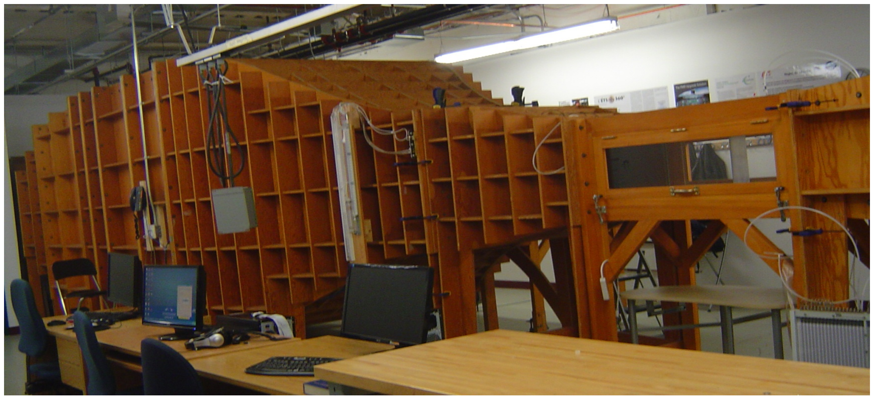
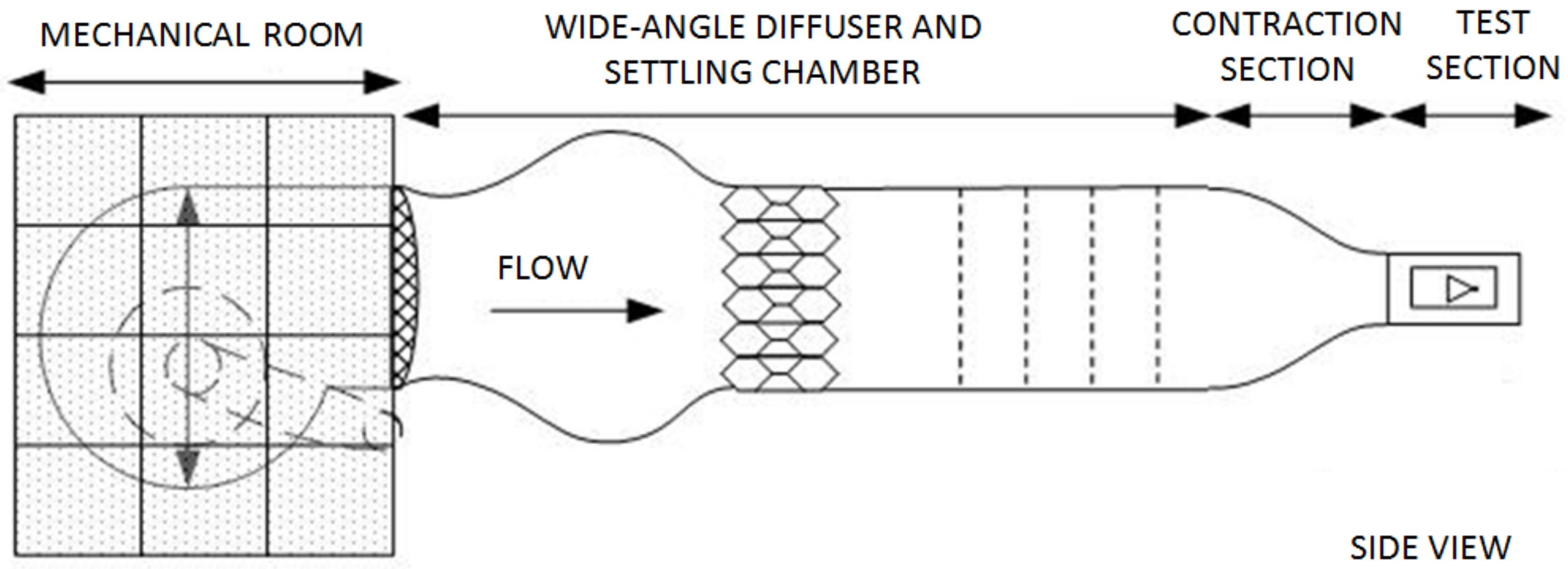
The Price-Païdoussis Open Return Subsonic Wind Tunnel shown in Figure 2 is a research apparatus for the validation of Computational Fluid Dynamics (CFD) models of various geometrical shapes and dimensions. The wind tunnel consists of a centrifugal fan, a diffusing and settling chamber, a contraction section, and a test chamber or test section, as shown in detail in Figure 3. The air supply enters the wind tunnel by two inlets located on opposite sides of the centrifugal fan. The engine and the centrifugal fan are protected from dust particles inside a closed area.

An important step to perform before experimental tests is the “calibration phase”, in which the flow conditions inside the test chamber are obtained. The main parameters to characterize the flow during a wind tunnel test are: (1) the total, static and dynamic pressures; (2) the temperature variation during the test; (3) the controlled flow speeds, and finally the Reynolds number. The internal filters shown in Figure 3 are dissipating the flow turbulence, and the laminar flow enters the contraction section where the flow speed increases. The large test chamber for full-scale models has a height, width, and length of 1.5 × 2 × 4 m, respectively, a maximum speed given by Mach number M = 0.05, and a maximum Reynolds number of 10⁵.

The “aerodynamic scale” was designed and built in-house. It has three strain gages that convert force into ‘electrical resistance’, which can be used to measure forces and moments values in all three coordinates. The output signal from strain gages is amplified and filtered, and the overall noise is minimized. The LARCASE aerodynamic scale can measure Fx and Fy forces up to 2500 N with an accuracy of 1/2N and can support full-scale models with an Fz of up to 6250 N with an accuracy of ¾ N. The maximum values of Mx, My, and Mz moments are 400 Nm with an accuracy of 1/20 Nm. The radar was fixed to a pan/tilt device by use of eight screws, which lead to a ground clearance of 0.38 m and 360° operational range. The scale can measure three forces (lift, drag, and side) and three moments (pitch, roll, and yaw) and it was mounted between the pan/tilt device and a high-grade steel tripod screwed to the floor. The pan/tilt device allows the variation of the yaw angle within ±0.01°. Two circular aluminum plates were used as interfaces and manufactured for this study. They were rigidly coupled to align the pan/tilt device, the aerodynamic scale, and the tripod. The pan/tilt device is a cube with a constant surface area on its front, back, and both sides [34].

The temperature and pressure readings are important for calculating the air density and flow speed during wind tunnel tests. The sensor used in the wind tunnel for measuring the temperature is a thermocouple type K with its accuracy of ±0.5 per degree Celsius. The Pitot tube inside the test section measures the flow static and the total pressures. The holes on the Pitot tube surface that are perpendicular to the speed direction are used for static pressure measurements, and the hole at the tip of this tube is used for total pressure measurements [35].

A multifunction data acquisition system USB-6210 from National Instruments (NI) was chosen to convert the analog signals of the aerodynamic scale into digital during the wind tunnel tests, and further to save them for their post-processing. The USB-6210 allows measurements of up to 16 analog inputs and does not require external power for its functioning. It reduces all input signals to a single USB cable, and can thus send the data from the force sensors to a remote PC. A custom interface was designed to acquire, visualize, and save data for post-processing. A video film was also recorded during the wind tunnel tests by use of the camera installed inside the test section. The aerodynamic data saved for each wind tunnel test were later imported in MATLAB 9.0 (2016b) for their analysis in the research post-processing phase. Each wind tunnel test was done at a sampling rate of 1000 Hz for pressure and temperature sensors, and 10,000 Hz for force and moment sensors.

5. Experimental Approach

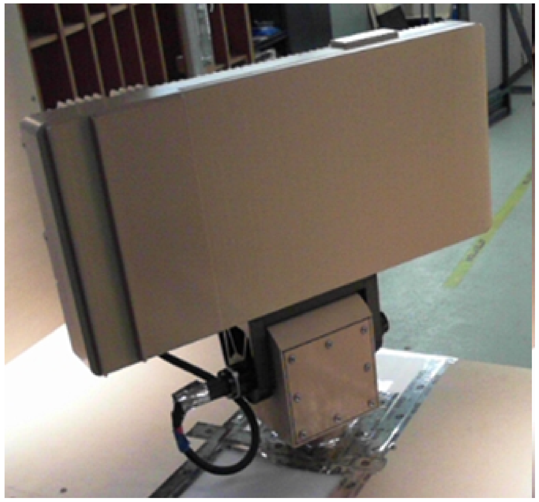
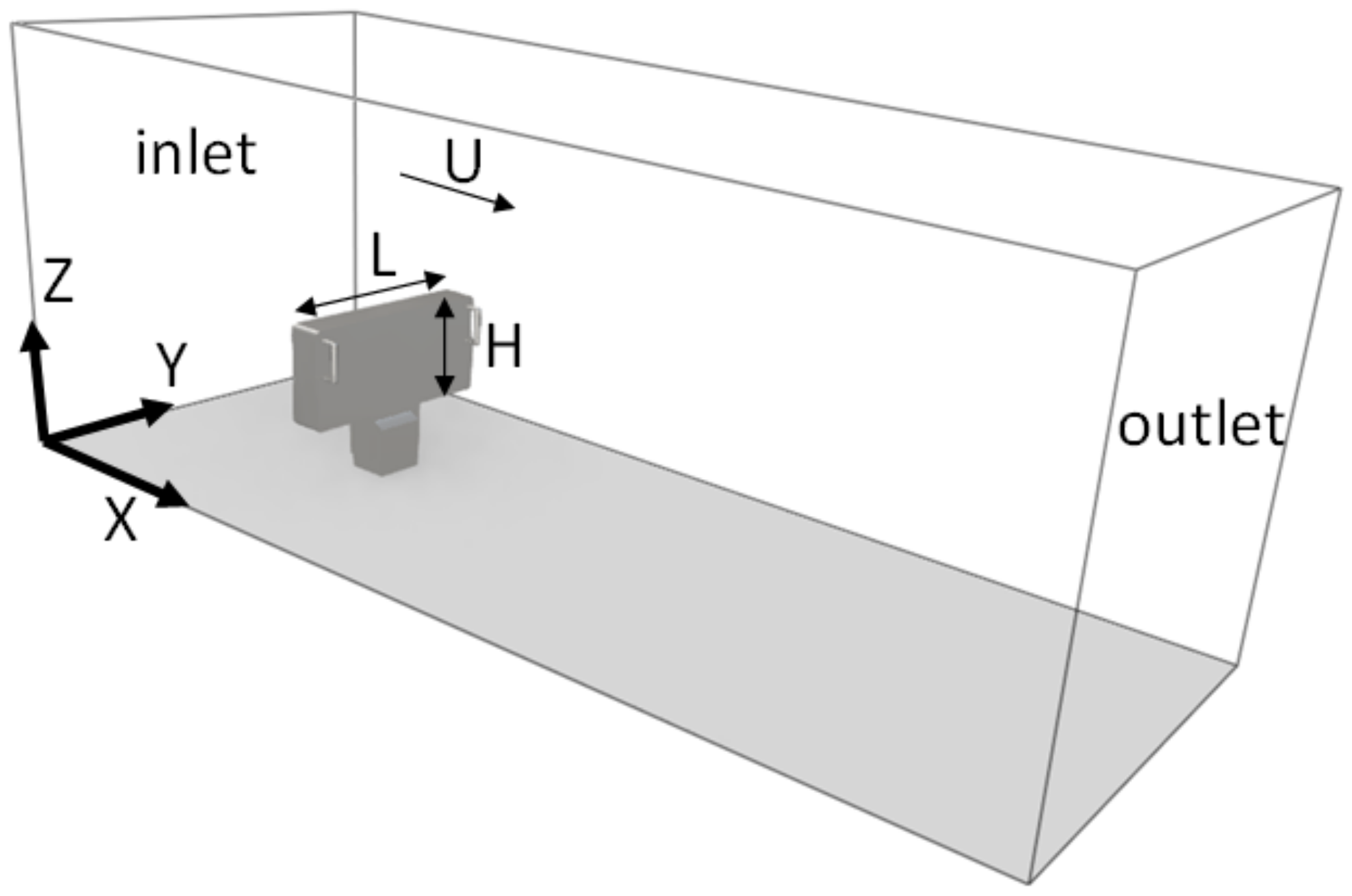
For each wind tunnel test performed for this research, the authors measured and recorded the values of forces, moments, shedding frequencies, pressure, and velocity variations at the wake region of the radar. Before performing experimental tests, a structural analysis was done to evaluate the stress distribution on the radar at the flow speed of 15 m/s. The photograph of the radar tested at the LARCASE wind tunnel is illustrated in Figure 4. The dimensions of the radar are the following: the height H = 0.37 m, the length L = 0.75 m, and the thickness h = 0.16 m. The projected frontal area of the radar is A_m = 0.278 m² with an aspect ratio AR = H/L = 0.49. Experimental tests were conducted at the Price–Païdoussis subsonic wind tunnel in its 1.5 m × 2.0 m × 4.0 m test section with a frontal surface area A_wt = 3.0 m². The positions of the yaw angle were denoted by γ as they measured the angles in degrees between the airflow direction and the frontal area of the radar. The angles are positive in are oriented in the clockwise direction. An angle γ = 0° indicates that the radar maximum surface A_m is perpendicular to the flow, and an angle γ = 90° indicates that the radar maximum surface rotates towards the right side wall of the test section while the radar’s smaller surface (side of the radar) is perpendicular to the airflow direction.

The radar was located at the center of the test section, where the blockage ratio $\frac{A_m}{A_{wt}}$ is equal to $\frac{0.278}{3.0}$ = 9.27% for γ = 0°.

5.1. Empirical Equations

The flow speed $U$ was determined by using the air density $\rho$ and the difference between the total pressure $P_t$ and the static pressure $P_s$, as shown in the Bernoulli equation [36].

$$P_t-P_s=q_c=\frac{1}{2} \rho U^2$$

(3)

The Reynolds number [36] $R{e}_H$ was calculated using the wind tunnel speed U, the radar height H, and the constant air kinematic viscosity $\vartheta \left(T\right)$ at T = 22°:

$$R{e}_H=\frac{UH}{\vartheta \left(T\right)}$$

(4)

The drag coefficient [36] $C_d$ is a non-dimensional form of the drag force $F_d$ acting on the radar body and in the flow opposite direction. Equation (5) of the drag coefficient is given next:

$$C_d=\frac{2F_d}{\rho \left(\mathrm{T}\right)U^2{A}_m}$$

(5)

As the flow acts on the radar in the wind tunnel test section, a constraint occurs in the flow at the wake region. Equation (6) proposed and verified experimentally by Garner and Maskell [37] captures the blockage effects on bluff bodies. To determine the aerodynamic coefficients $C$ without taking into account the constraints of the wind tunnel test section walls, the values of the uncorrected aerodynamic coefficients [37] $C_u$, the blockage ratio $\frac{A_m}{A_{wt}}$ and the empirical value ω need to be calculated. Therefore $C$ is obtained using the next equation:

$$C=\omega C_u\left(\frac{A_m}{A_{wt}}\right)$$

(6)

The blockage factor for blunt-body [37] ω is an empirical value describing the effects of the rigid walls, and those of the blunt body stopping the flow lateral displacement. The ω value is calculated based on the pressure coefficient $C_p$ as follows:

$$\omega =\frac{1}{\left(1-C_p\right)2-1}$$

(7)

The pressure coefficient $C_p$ is a non-dimensional ratio between the local static pressure differences and the dynamic pressure of the incoming flow. The local static pressure $P_i$ is evaluated at various locations in the test section. The pressure coefficient $C_p$ measures the local static pressure relative to the freestream static pressure $P_s$ and the freestream dynamic pressure $q_c$. The pressure distribution is therefore calculated with the following equation:

$$C_p=\frac{P_i-P_s}{q_c}$$

(8)

The dynamic pressure increase at the wake region produces a local reduction of the static pressure; therefore, the correction $C$ presented in Equation (6) is applied to the aerodynamic coefficients $C_u$. The corrected $C$ values are given by the following equation:

$$C=0.942 C_u$$

(9)

The turbulence intensity I is the ratio between the velocity variation in the flow local components $u_x$, $u_y$, and $u_z$ and the free stream velocity U inside the wind tunnel test section. The turbulence intensity values I were calculated with the following equation:

$$I=\frac{{(u_x+u_y+u_z)}^2}{U^2}$$

(10)

The Strouhal number (St) is the most important parameter associated with periodic vortex shedding, flow oscillations, and turbulence kinetic energy production at the wake region for blunt bodies [38]. At St ≥ 0.3, the flow is fully turbulent and dominated by periodic vortices shedding. For an intermediate range of Strouhal number 0.2 ≤ St ≥ 0.3, oscillations and periodic motions appear, and a turbulent wake forms behind the blunt body. At low Strouhal numbers (St ≤ 0.2), the oscillations and vortices are dissipated by the moving fluid. St is defined by the vortex shedding frequency f, the length H, and the free stream flow velocity U. The St value is calculated with the following equation:

$$St=\frac{fH}{U}$$

(11)

5.2. Experimental Data

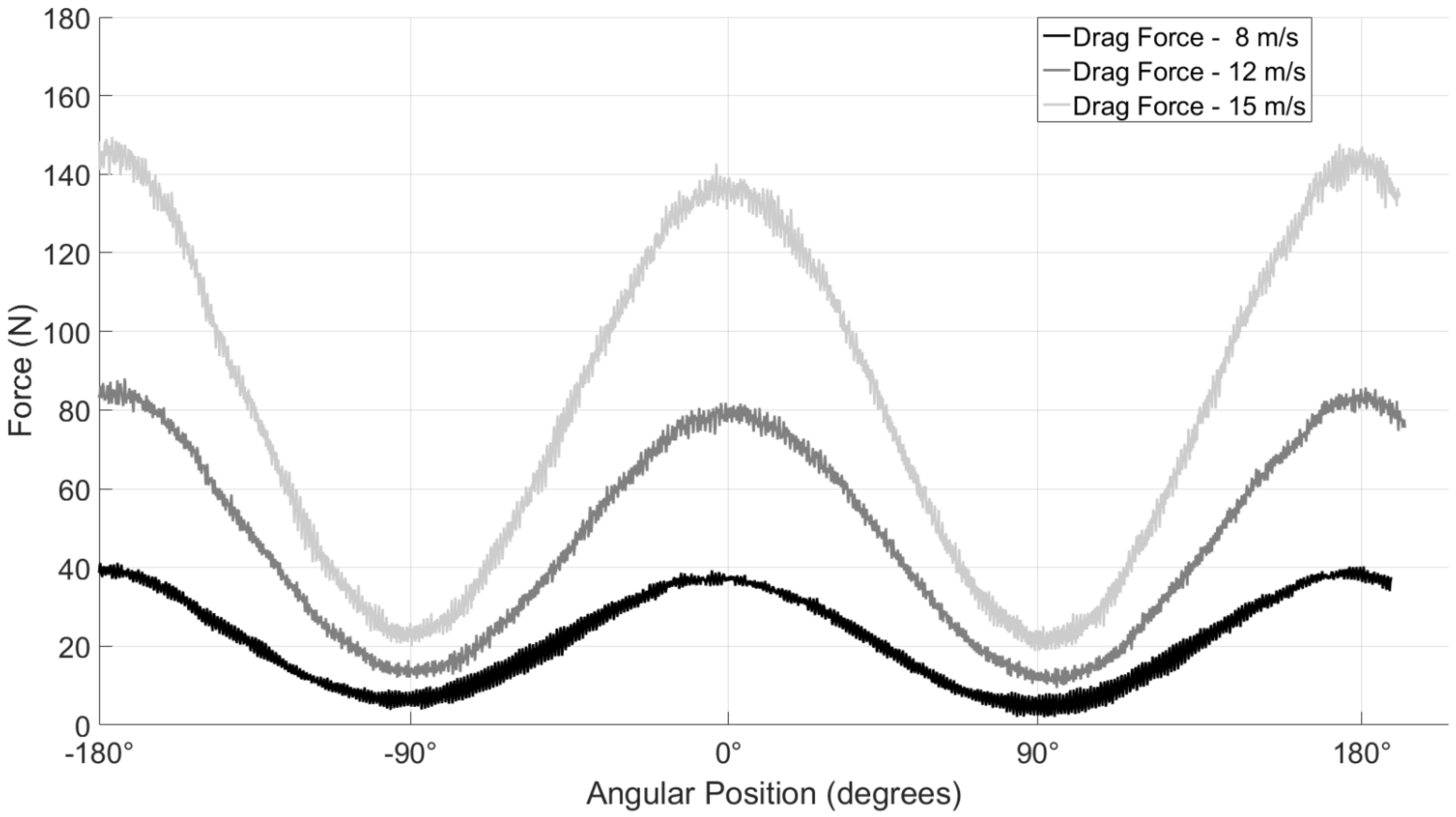
The experimental data were collected in real-time as the radar changes its angular position. The unfiltered drag forces obtained for three flow velocities are presented in Figure 5. The drag force has a maximum value at γ = 0°, and has its minimum value at γ = 90°. It can be mentioned that as the cross-section surface of the radar decreases with the angular position γ, the drag force exerted on the radar body decreases independently of the flow speed. Figure 5 also shows the blunt body symmetry between its front and rear sides, as well as between its left and right sides.

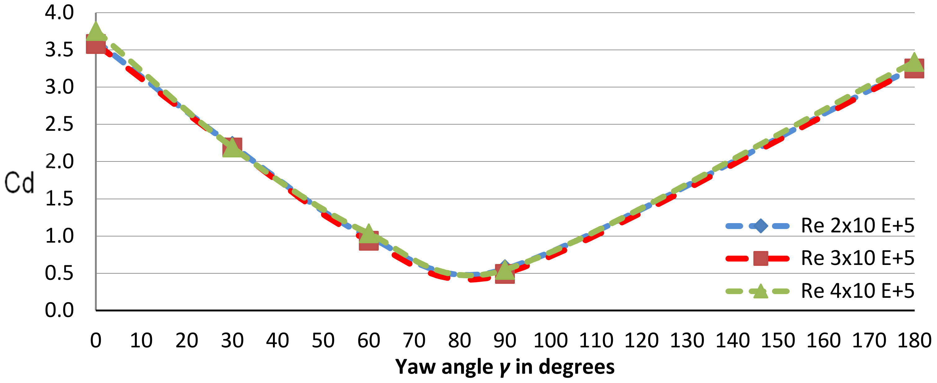
For blunt bodies, the drag coefficient is independent of the Reynolds number because of the fact that in a turbulent flow regime, the wake region is dominated by sharp edges and blunt body shapes^. The drag coefficient values variations were obtained using Equations (5) and (9) and they are presented in Figure 6. The experimental drag coefficient values were found to be close for each angular position, which meant that they were independent of the Reynolds number. Their non-dependence on the Reynolds number allowed the design and analysis of a system able to decrease the drag force for any flow speed encountered by the radar.

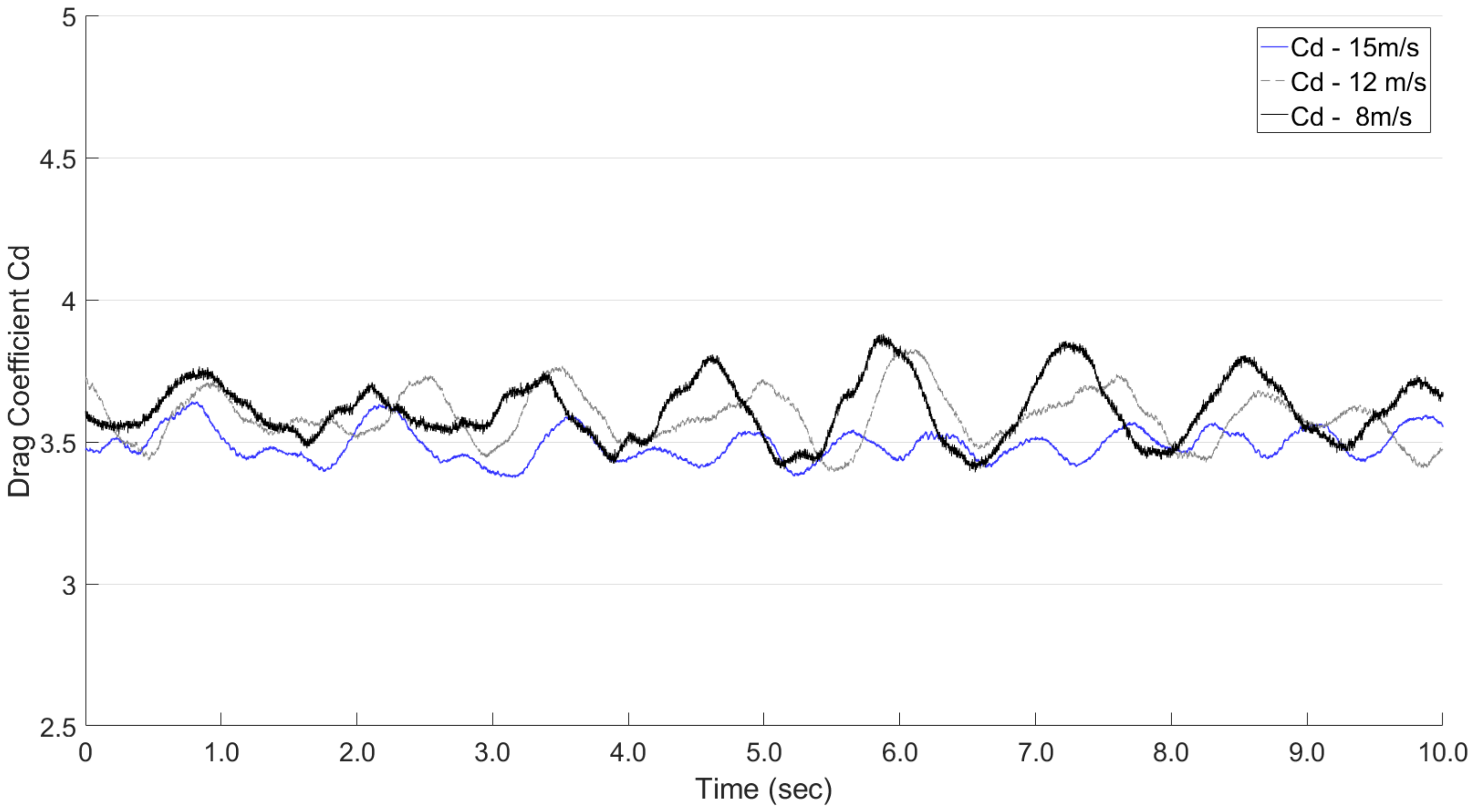
Periodic oscillations are present in the streamwise loads for the three flow regimes tested during the wind tunnel test of the radar. The experimental load Fx is characterized by a periodic motion, associated with oscillations in the wake region and provoked by the constant boundary layer separation at the upper surface of the radar, and by changes in the velocity of the flow field. Figure 7 presents the drag coefficient of the force Fx variation with time at the angular position γ = 0° collected for 10 s and for three flow velocities: 8, 12, and 15 m/s.

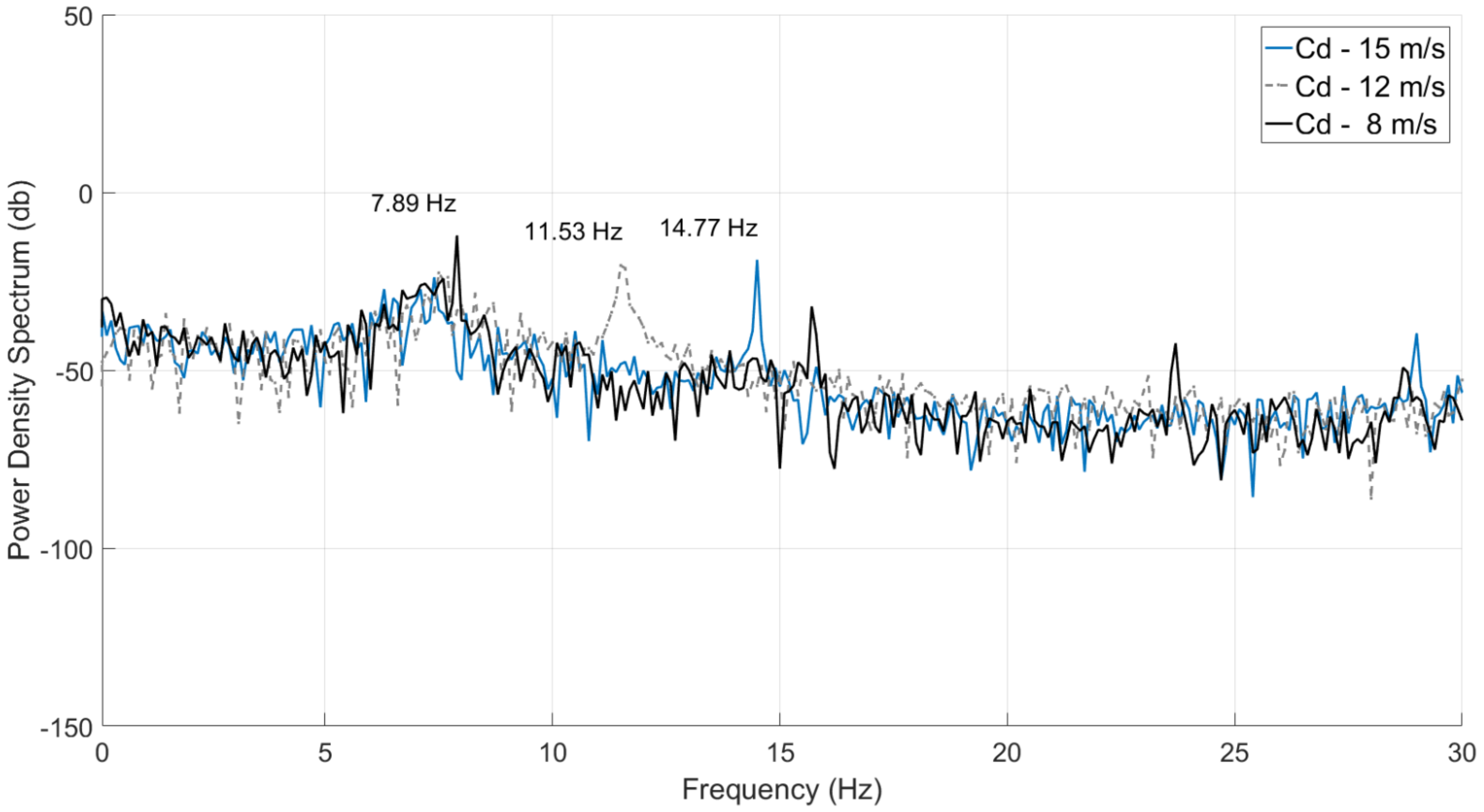
The Strouhal number (St) describes turbulent periodic flow characteristics of blunt bodies. The oscillations for the drag forces are composed of a spectrum of frequencies. To find the frequency distribution for each flow velocity, the drag coefficients values shown in Figure 7 are decomposed in discrete frequencies as seen in Figure 8, where the power spectrum for each drag coefficient is traced versus frequency. The fundamental frequency presented in the flow at a velocity of 8 m/s is 7.89 Hz; at a velocity of 12 m/s is 11.53 Hz and at a velocity of 15 m/s is 14.77 Hz. Using the dimensionless Strouhal number defined in Equation (11), the radar’s dimension normal to the flow direction H = 0.37 m and the fundamental frequencies for each wind tunnel test, the St number representing the vortex shedding on the radar blunt structure had three values $S{t}_{8\mathrm{m}/\mathrm{s}}=0.365; S{t}_{12\mathrm{m}/\mathrm{s}}=0.356$ and $S{t}_{15\mathrm{m}/\mathrm{s}}=0.364$. As a Strouhal number St ≥ 0.3, we can conclude that the wake region of the radar is turbulent and unsteady while flow separation and vortices shedding downstream occur.

6. Numerical Approach

The full-scale radar, the Price–Païdoussis subsonic wind tunnel, and the flow around the radar were all modeled, meshed, and solved using ANSYS Fluent. This section shows in detail the numerical approach needed to obtain the radar aerodynamics coefficients; also, it shows the verification and validation process following the ASME guidelines.

6.1. CFD Models Design and Grid Domain

The physical dimensions and shapes of the test section and the radar were used to design a numerical representation of these two models. The aerodynamic scale measures the forces and moments at the base of the radar system; therefore, the moments are calculated at the same location as the forces. The meshing process includes the next steps: (a) the design of an initial mesh, followed by an evaluation of its quality, and by specifications of its boundary conditions; (b) the improvement and repairing of the mesh discontinuities and space between its cells; (c) the generation of the volume mesh using Triangle and Quad elements and refining of the mesh density close to its boundary layer; (d) the exportation of the final mesh to a neutral format. Two meshes were designed separately and then merged into a single mesh for its use in the Finite Element Analysis and Computational Fluid Dynamics solvers.

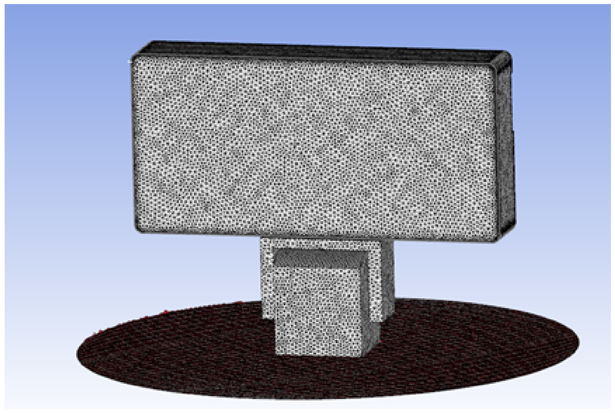
The CAD of the original radar has been prepared for meshing by eliminating small details on the radar’s surface. The y⁺ value was an important parameter for mesh-size calculation in the near-the-surface-mesh design with a growth rate of 20% for the next mesh layers. The radar mesh at its surface was composed of 130,580 unstructured mesh elements; 97% of these elements were modeled by triangular prisms. The radar face and rear meshes can be seen in Figure 9.

A mesh with a higher resolution was designed around the radar to accurately capture the turbulent wake at the rear of the radar. The 3D mesh was called ‘InnerFluid’, and it was composed of 2,583,142 prisms and tetra unstructured mesh elements. To ensure an accurate simulation of the boundary layer flow near the model, 15 prism layers were used with the y⁺ calculated value as the first mesh size. The grid independence tests were performed with coarse, medium, and fine meshes; the forces and moments were not dependent on the mesh resolution [39,40].

The numerical model of the radar was constrained by four wall regions and two pressure regions (inlet and outlet) to simulate the flow conditions during wind tunnel tests. The flow direction, the radar position inside the test section, and the reference axis are shown in Figure 10.

6.2. Boundary Layer Region Thickness

Speed gradients are important for enclosed domains, such as wind tunnels, where the mesh resolution and number of inflation layers are critical [41,42]. The flow mesh inside the wind tunnel section was called ‘Inner_Fluid’ in the CFD software. An accurate mesh size and number of layers at the boundary layer near the four walls of the test section were needed to accurately simulate and describe the flow behavior in this region.

The resolution and size of the mesh (cells heights forming the mesh) and the number of cells-layers at the boundary layer were important for the turbulence model to accurately find the speed profile and further to predict the flow behavior. The CFD model allows modifying the mesh resolution and size, as well as the height of each cell by use of a non-dimensional distance y⁺. To accurately simulate a CFD model, the y⁺ distance must be calculated as a function of the (1) turbulence model, (2) Reynolds number defined by the experimental tests of the radar, and (3) flow behavior at the wake. In this study, the k-ε turbulence model was chosen to be used with Re > 10⁵ and a wake region experiencing flow separation, recirculation, and vortices [43,44].

The turbulence model k-ε recommends y⁺ = 300 to define the boundary conditions at the wall. Since it is difficult to gauge the near-wall resolution requirements for the size of the radar, the y⁺ value was estimated inside the wind tunnel test section by use of a semi-empirical equation provided by ANSYS Fluent documentation [45].

For this study, it was important to calculate the height of the boundary layer inside the wind tunnel test section for the same flow conditions as the ones of the wind tunnel tests. The density was set to ρ(22 °C) = 1.196 Kg/m³ and the dynamic viscosity was set to μ(22 °C) = 1.822 × 10⁻⁵ Pa × s. The Reynolds number was calculated with Equation (5) for 15 m/s at the location of the radar L = 5 m, thus $R{e}_L$ = 5 × 10⁶ was obtained.

The turbulence thickness $\delta$ at the location L was calculated with Equation (12):

$$\delta =\frac{0.382 L}{R{e}_L^{0.2}}$$

(12)

The turbulence thicknesses $\delta$ at the locations L = 2 m and L = 5 m were ${\delta }_{L=2}$ = 4 × 10⁻² m and ${\delta }_{L=5}$ = 9 × 10⁻² m. The skin friction coefficient for a turbulent flow $C_{ft}$ was calculated with Equation (13), thus $C_{ft}$ = 2.7 × 10⁻³ for $R{e}_L$ = 5 × 10⁶.

$$C_{ft}=\frac{0.0583}{R{e}_L^{0.2}}$$

(13)

The wall shear stress ${\tau }_w$ = 0.36 Pa was calculated with Equation (14).

$${\tau }_w=C_{ft}0.5 \rho U^2$$

(14)

The frictional velocity $U_{\tau }$ = 0.55 m/s was obtained by use of Equation (15).

$$U_{\tau }=\sqrt{\frac{{\tau }_w}{\rho }}$$

(15)

The estimated boundary layer thickness at the radar position had a height $\delta$ = 4 × 10⁻² m. Therefore 15 mesh layers were installed at the boundary layer region to ensure accurate grid inflation on the whole mesh. The total height $\delta$ = 4 × 10⁻² m of the boundary layer divided by 15 mesh gave the value y = 2.7 × 10⁻³ m for each mesh layer by use of Equation (16).

$$y=\frac{4\times {10}^{-2}}{15}$$

(16)

Then, Equation (17) was used to find $y^{+}$ for a cell height of y = 2.7 × 10⁻³ m.

$$y^{+}=\frac{\rho U_{\tau }}{\mu }y=96$$

(17)

Therefore, $y^{+}$ = 96 for the radar’s wake region.

6.3. CFD Model Simulation Characteristics

The flow around the radar changes over time from laminar to turbulent flow with its recirculation and vortices emerging in the wake region; as a result, the CFD model of the radar was solved using a transient flow simulation. The solver was designed to simulate with a high degree of accuracy the wind tunnel tests performed on the radar. In this paper, the pressure-based method was used as it was mainly developed for incompressible low Reynolds number applications (Mach numbers below 0.3); in fact, the Pressure-Implicit with Splitting of Operators algorithm was used as a pressure-velocity calculation procedure for solving the Navier–Stokes equations. A k-ε model coupled with the Detached Eddy Simulation (DES) and a wall function with the above-calculated value of y⁺ were chosen for the flow analysis. The inlet x-velocity was set to its desired speed during the wind tunnel tests (8 m/s, 12 m/s, and 15 m/s). During these tests, the speed variation across the empty test section was 1% while the turbulence intensity was 0.3%; these values were used in the turbulence model. The outlet gauge pressure was set to atmospheric pressure as the outlet pressure of the wind tunnel. The radar transient simulations were calculated for more than 22,500 iterations for each case (1 case is considered for 1 flow speed and 1 angular position of the radar). To have information on the flow time variation, the simulation step time was set to a value of 10⁻⁴ s. The simulation time converged to an accurate solution after 2000 time steps, which corresponded to a total time of 2000 × 1 × 10⁻⁴ = 0.2 s. The Residual Convergence criteria were set to a value equal to 1 × 10⁻⁵, to obtain accurate forces and moments values.

6.4. CFD Validation

This sub-section provides the validation requirements of the ASME guidelines described in Section 2.3. In total, 15 test cases were performed during wind tunnel tests, in which three forces (Fx, Fy, Fz) and three moments (Mx, My, Mz) were measured by our in-house aerodynamic scale. The radar and aerodynamic scale were mechanically connected by a non-permanent joint consisting of a bolt flange and 4 bolts (each bolt of a diameter of 10 mm). This joint has not allowed any motion in the Fz direction and has not allowed any Mz moment between the radar and the aerodynamic scale. The values measured by the aerodynamic scale were found to be very low, Fz = 0.002 N and Mz = 0.001 Nm. These Fz and Mz values were observed during experimental tests for safety reasons, to ensure that the radar and aerodynamic scale were fixed together. These values were not calculated by use of CFD as they were very low and have not provided any information on the interaction between the radar and the flow. The Fx, Fy, Mx, and My values were calculated by CFD as they were the most important loads in this research.

6.4.1. Linear Regression Method

Linear Regression analysis [46] is a statistical process that allows for an estimation of the order of difference between the model’s predicted values and its experimental values. The correlation magnitude between the experimental values and the predicted values can be quantified by calculating the Adjusted R² (R-squared) of the model. This value denoted the proportion of the variance in the experimental data that is predicted by the model data. An Adjusted R² of 1 indicates that the model predicts very well all experimental data, but practically models are never perfect, therefore an Adjusted R² has any value between 0 and less than 1. The Adjusted R² values were 0.9986 for Fx, and 0.9945 for Fy, therefore the prediction for Fx was 99.86% and for Fy 99.45%. The moments Mx and My have an Adjusted R² of 98.29% and 98.26% respectively, which suggested a very good agreement between the experimental data and the simulated data.

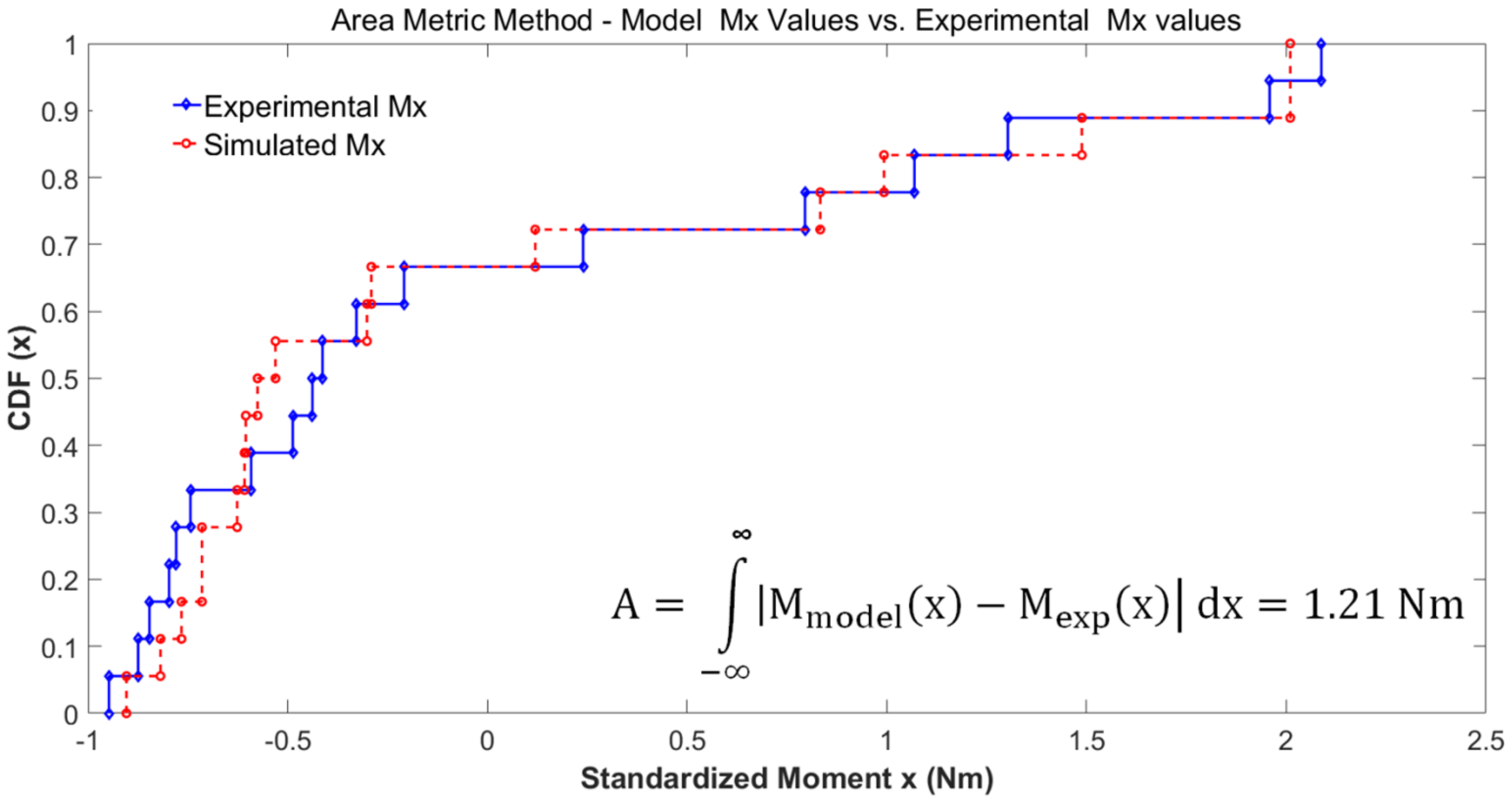
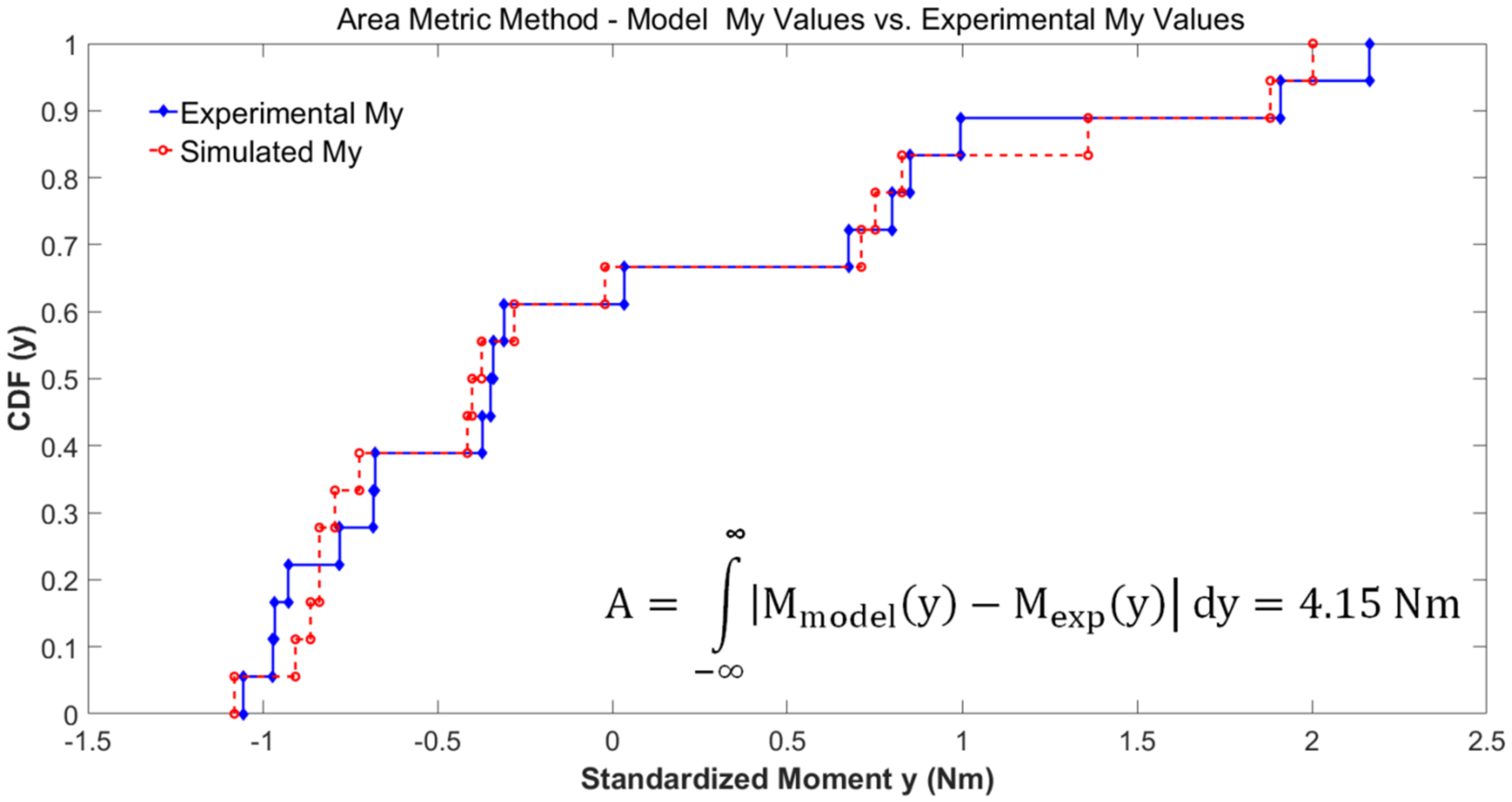
6.4.2. Area Metric Method

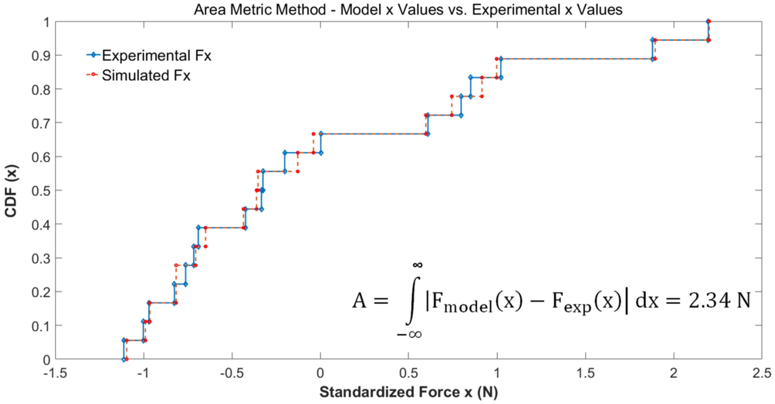
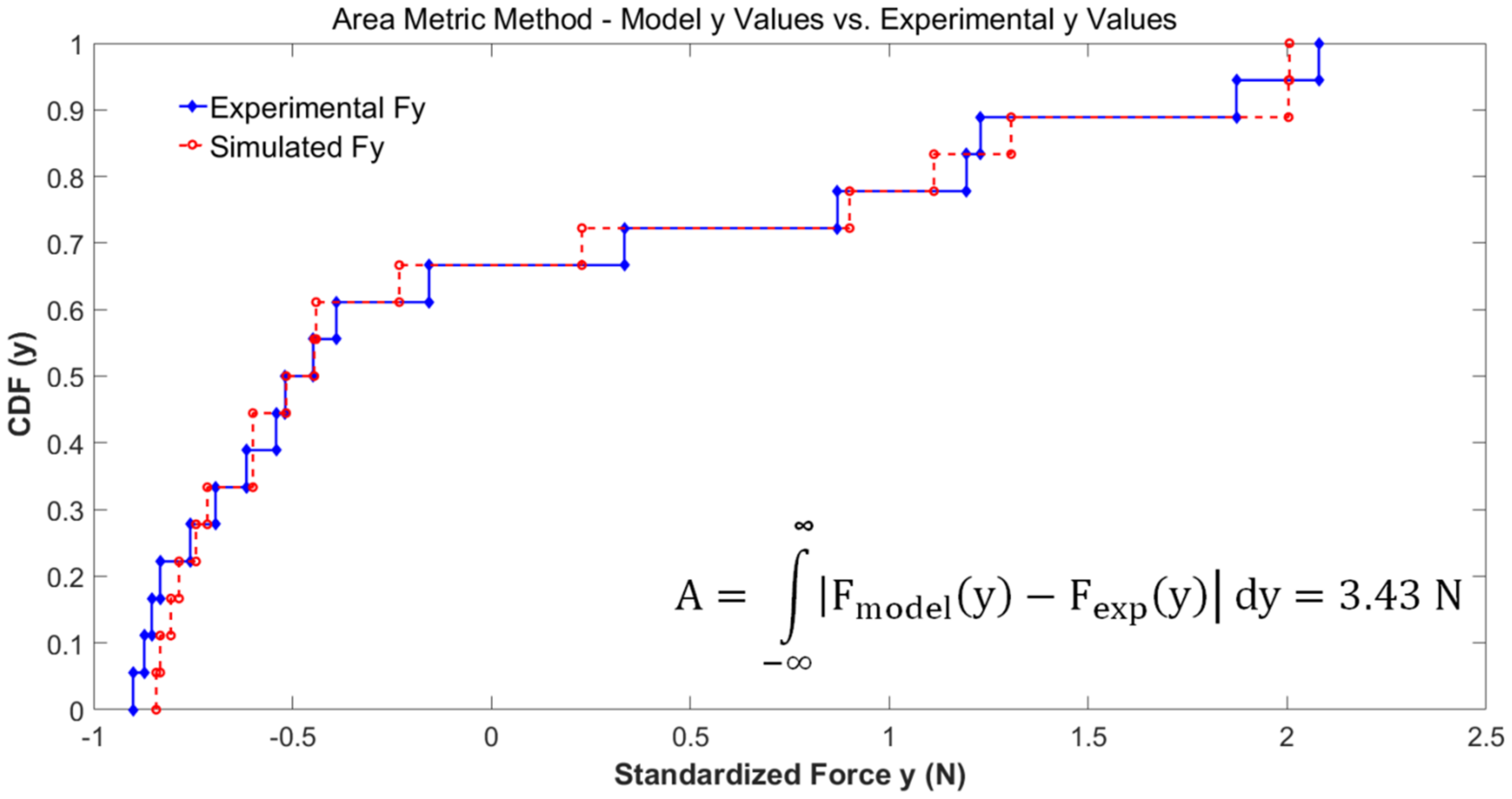
The Area Metric method [46] is part of the validation process required by the ASME guidelines when numerical models are used. This second type of validation measures the agreement between the simulated data and the experimental data by calculating the mismatch of the surface area between the two sets of data. The fact that this method allows validating a model when only a few experimental values can be measured is an advantage over other available validation methods. All experimental values were compared with the simulation values using the Area Metric method, as shown in Figure 11. This method measured a maximum difference of 2.34 N between the predicted Fx forces and the observed Fx forces. The Area Metric method, in a similar way, provided differences for Fy, Mx, and My which were respectively 3.43 N, 1.21 Nm, and 4.15 Nm, as shown in Figure 12, Figure 13, and Figure 14, respectively.

In conclusion, drag forces Fx were predicted very well with an accuracy of 99.86% (Linear Regression), and with a small mismatch of 2.34 N using the Area Metric Method.

7. Flow Analysis and Discussion

Literature review suggests that the flow behavior near blunts bodies have distinctive and recognized features contrasting those of streamlined bodies. Following flow disturbance on the blunt body, its motion can either continue developing its turbulent behavior at the wake or it can be damped by means of a turbulence reduction system. The CFD results have allowed analyzing the boundary layer behavior and unsteady wake flow region of the original radar and the radar with the turbulence reduction system. Figure 15 shows the main locations affecting flow behavior, the initial contact of the fluid with the upper surface of the radar, denoted by position 2, was called “leading edge” and the final contact point, denoted by position 4, was called “trailing edge”. The radar surface where most turbulence fluctuations occurred was called “upper surface” and represented by position 3. The “front region” and “rear region” are denoted by positions 1 and 5, respectively.

7.1. Original Radar Flow Analysis

The validated CFD model gave new insights to study the fluid in contact with the radar surface from its boundary layer separation to vortex formation and turbulent transition. This section describes the transitional state where a laminar flow interacts with a blunt body by provoking boundary layer separation, vortex formation, and flow instabilities. When the flow approached the radar blunt body, there was an increase in dynamic pressure at its upper surface and a sudden decrease in static pressure at the “front region” and at the “rear region”. The rapid increase in dynamic pressure at the upper surface of the radar produced a vacuum in the wake region shown in Figure 16 in blue color. As the flow moved forward, the main recirculation region started to form with a high rotation dynamic energy shown by red, yellow, and green colors. The fluid at the front and the rear of the radar moved slowly with respect to the rest of the flow by provoking the boundary layer to separate abruptly at the “leading edge”. The high flow velocity and dynamic pressure at the upper surface increased the turbulent energy in the wake region.

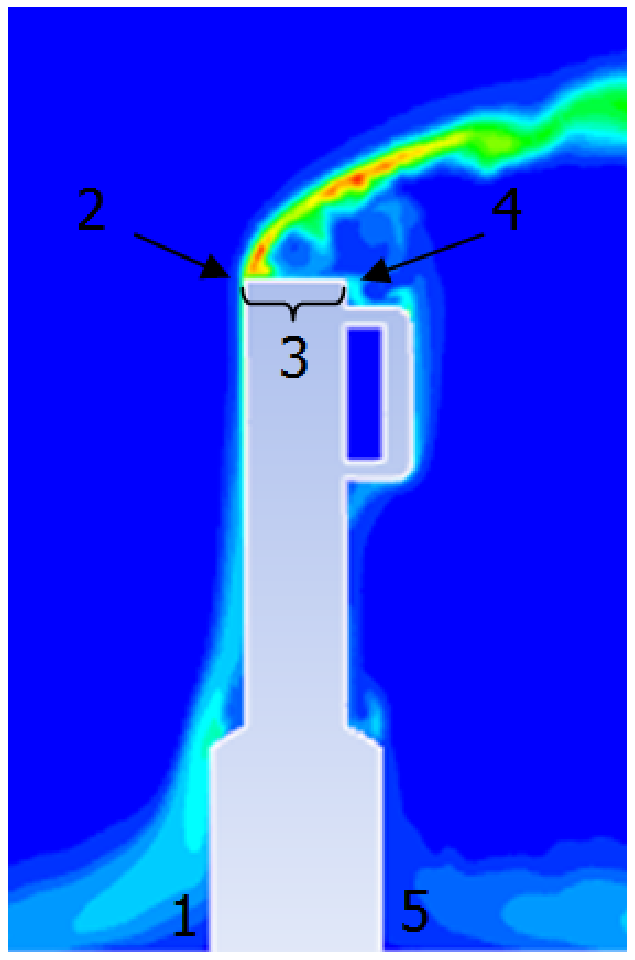
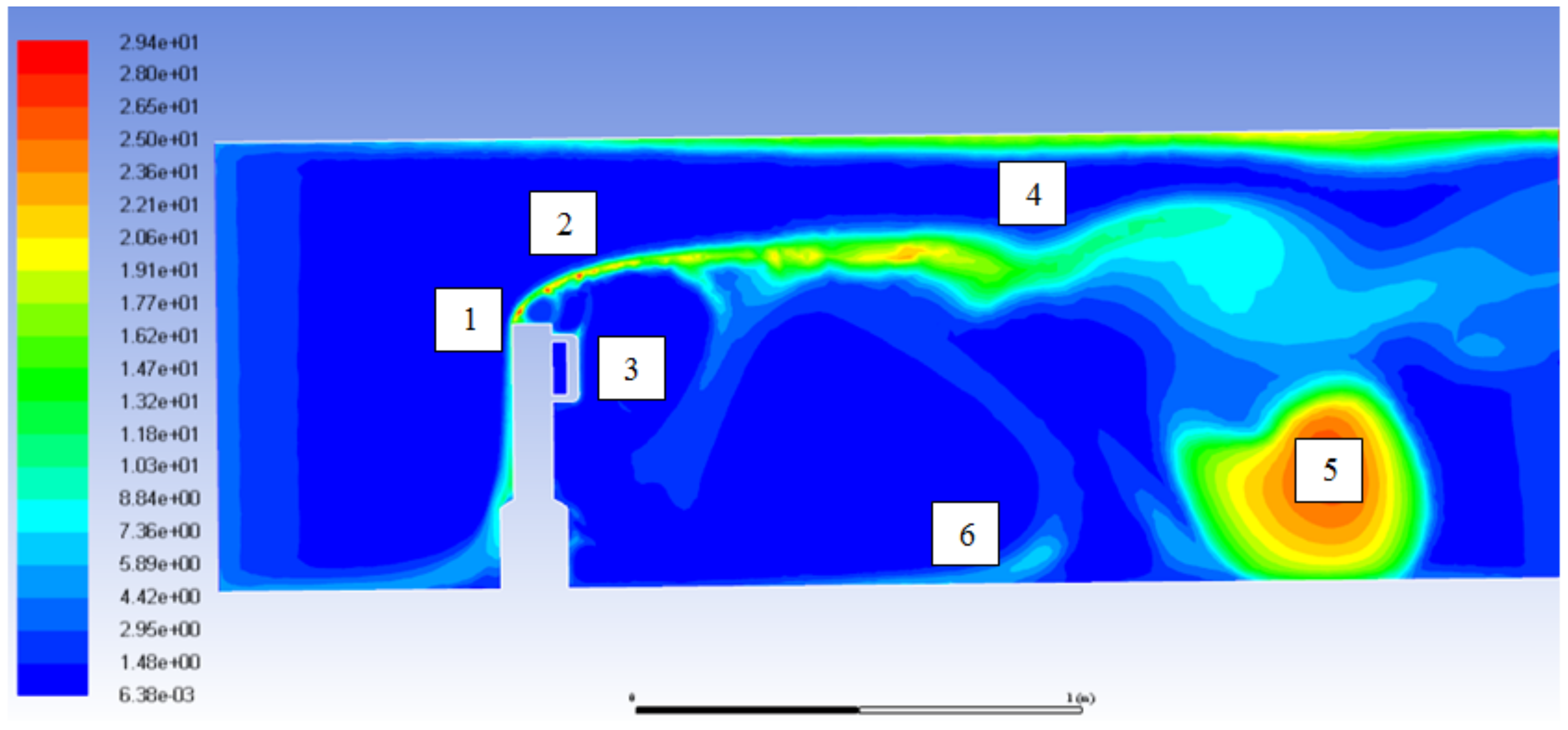
It is known that the flow surrounding a blunt body is mainly formed by pressure drag, and a small fraction of it is due to friction drag. The flow structure seen in Figure 17 contains the major components of a turbulent flow calculated with fluctuations of the mean flow speed, as described by the turbulence intensity I in Equation (10). In Figure 17, at position 1, the flow separates from the radar surface, and the flow transitions to its turbulent state with its intensity close to 20.6%. At position 2, the separated shear layer gain momentum, and small irregular eddies appear with a high-intensity ratio I = 29.4%, as seen at position 5. High intensities regions are representing velocities fluctuations and vortices. The flow tries to reattach to the radar’s upper surface and also to its rear handles as shown at position 3. The main recirculation region is formed at a distance of 1 m from the radar location. The high velocities gradients at the wake and close to the upper wall (of the test section) are shown in green and yellow colors with their intensities ranging from 10% to 20% at position 4. At the main recirculation region, the high kinetic energy generates a vortex with a high turbulence intensity ranging from 10% to 29.4%, as shown at position 5. It is known that multiples recirculation regions occur on blunt bodies inside wall-bounded flows, as shown at position 6.

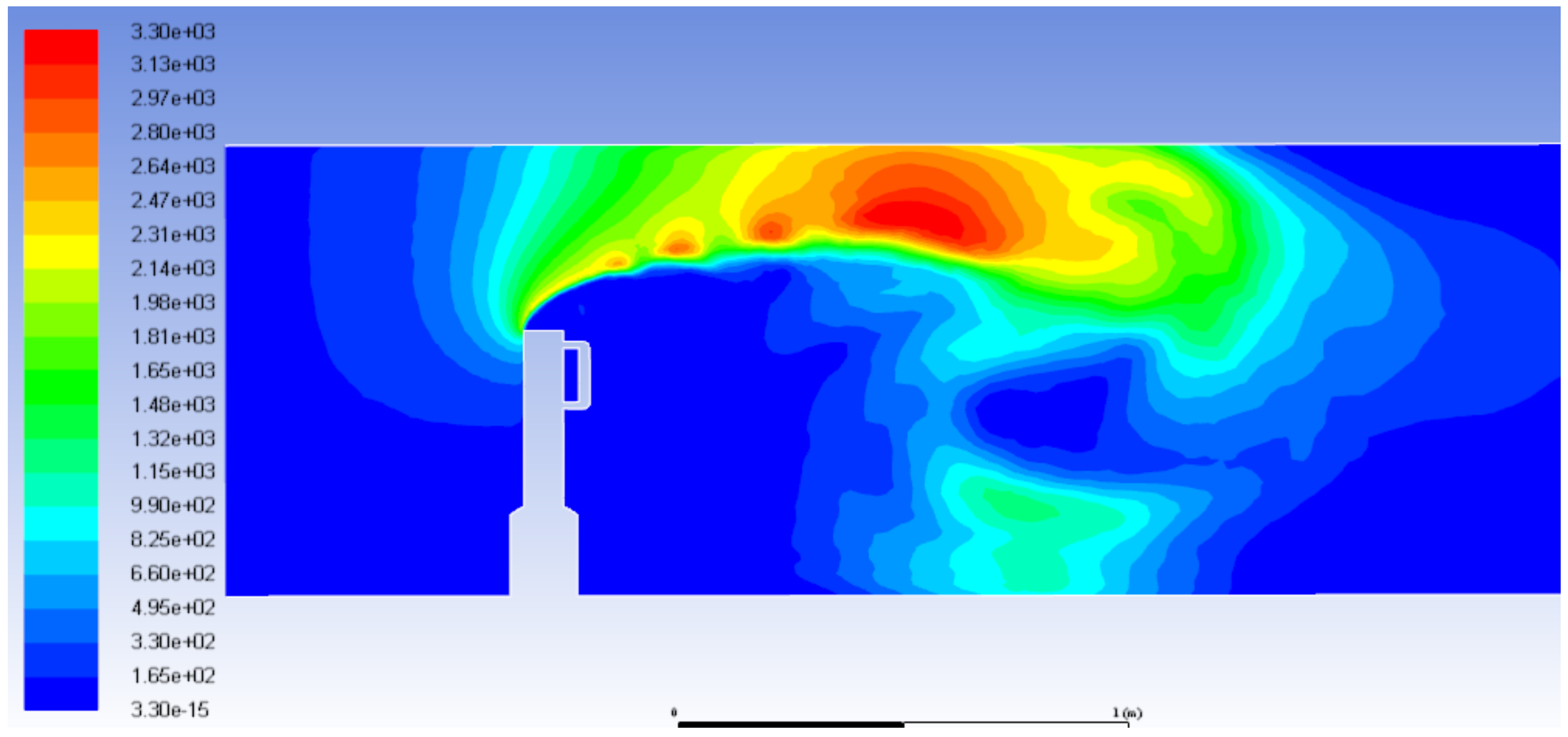
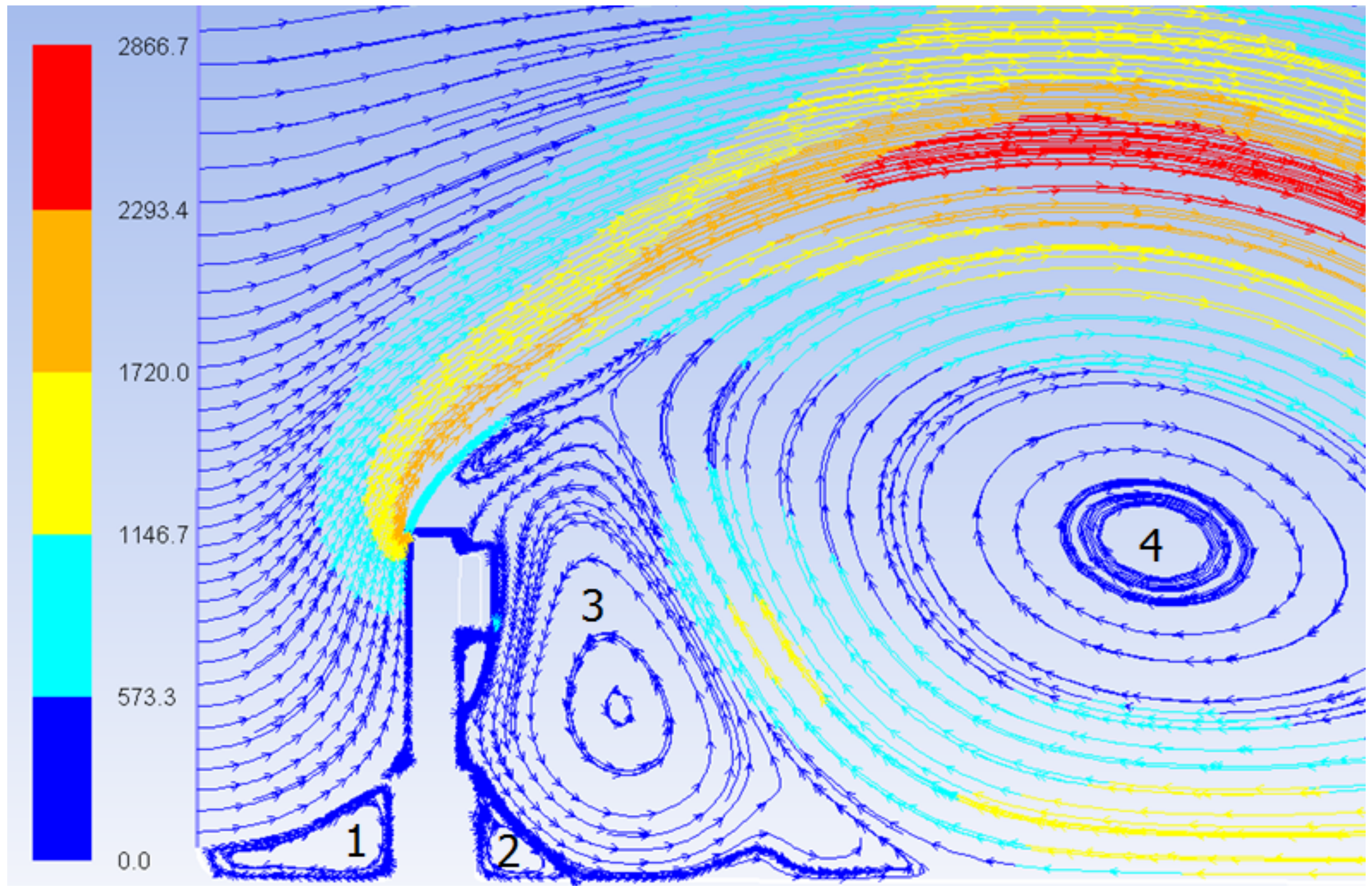
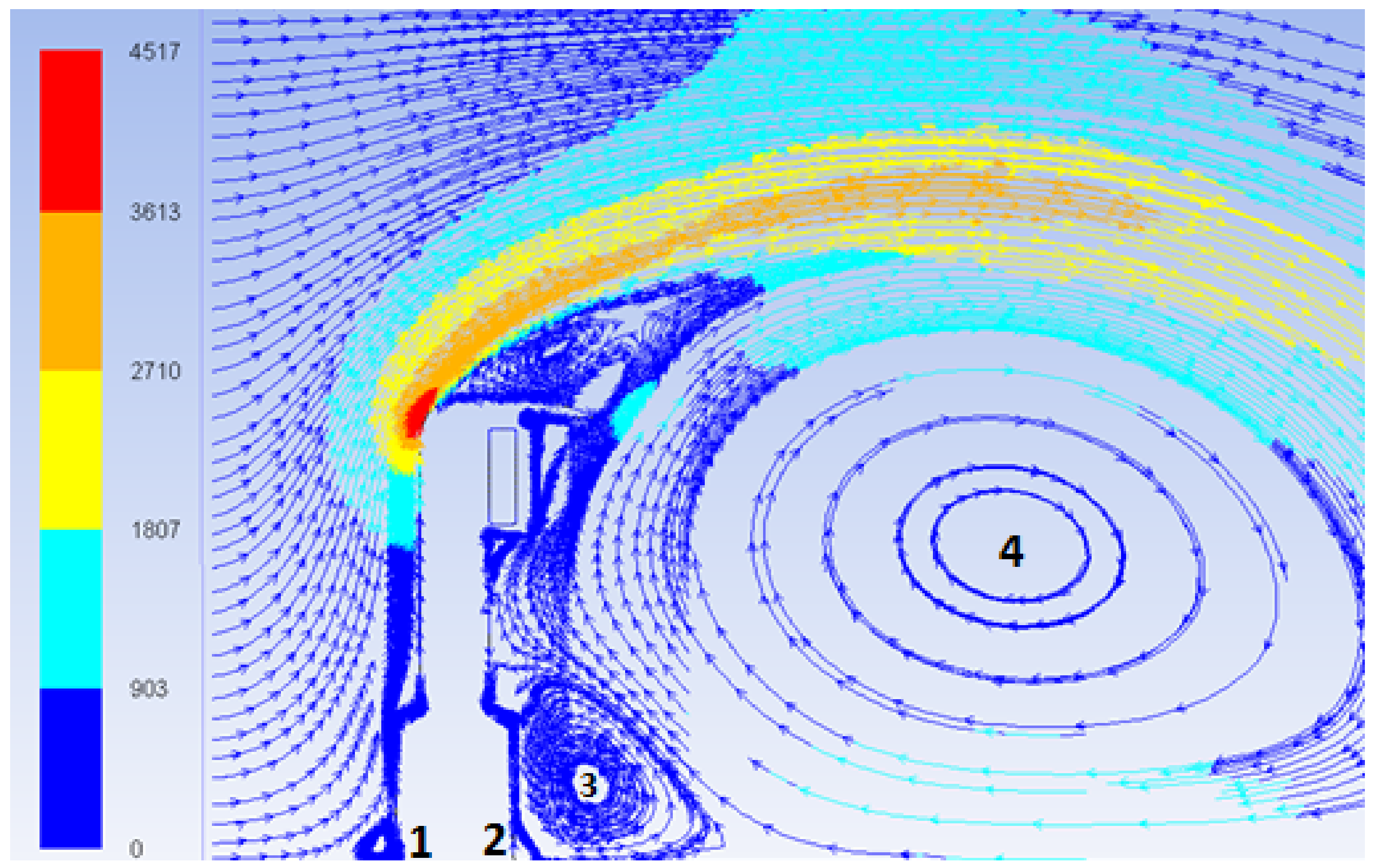
Immediately after contact with the blunt body, the fluid had changed to a fully turbulent flow. Figure 18 shows the streamlined directions and magnitudes of the fluid dynamic pressure field in the wake of the radar body. Initially, the flow separates abruptly at the “leading edge” of the radar due to a high range of dynamic pressures shown by cyan, yellow and orange colors in Figure 18; these high-pressure fields prevented the boundary layers to re-attach to the “upper surface” and thus, to produce two recirculation regions; the first recirculation region, shown by number 3, was attached at the rear of the radar surface, with the same diameter as the height “H” of the radar. The angular kinetic energy was not higher compared to that of the rest of the fluid in the wake region, but the local rotation was oriented in the opposite direction of the incoming flow (counter-clockwise rotation). The second recirculation region, shown by number 4, had a diameter three times higher than the height of the radar “H”, it was located at two lengths “H” from the rear of the radar, had high clockwise rotational direction and up to five times (2866/573 = 5 times) the dynamic pressure higher compared to the dynamic pressure of the rest of the flow. The pressure distribution at the front and back of the radar’s base produced two separation bubbles identified by number 1 at the “front region” and by number 2 at the “rear region”. The dynamic pressures, in these regions, were low and close to the stagnation pressure and local flows were moving in the clockwise direction.

The impact of the accelerated fluid on the surface of the radar has increased the turbulence production in the wake region; this flow transition to a turbulent regime can be observed and analyzed at the “upper surface” of the radar body. The original shape of the “upper surface” of the radar did not dissipate well the energy produced by the impact of the fluid with a blunt body into the fluid “kinetic energy”, therefore it created fluctuating instabilities and increased turbulence production.

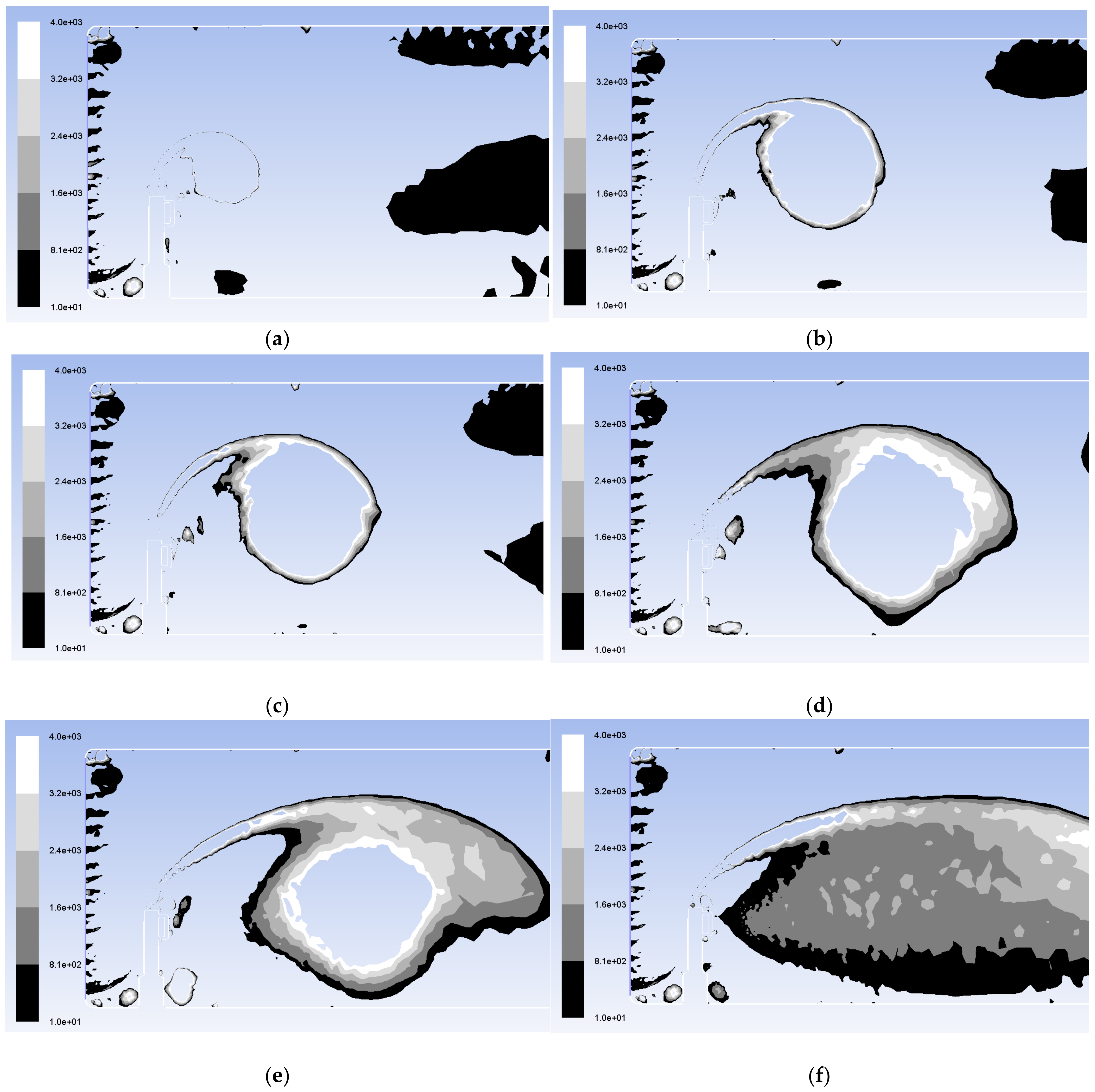
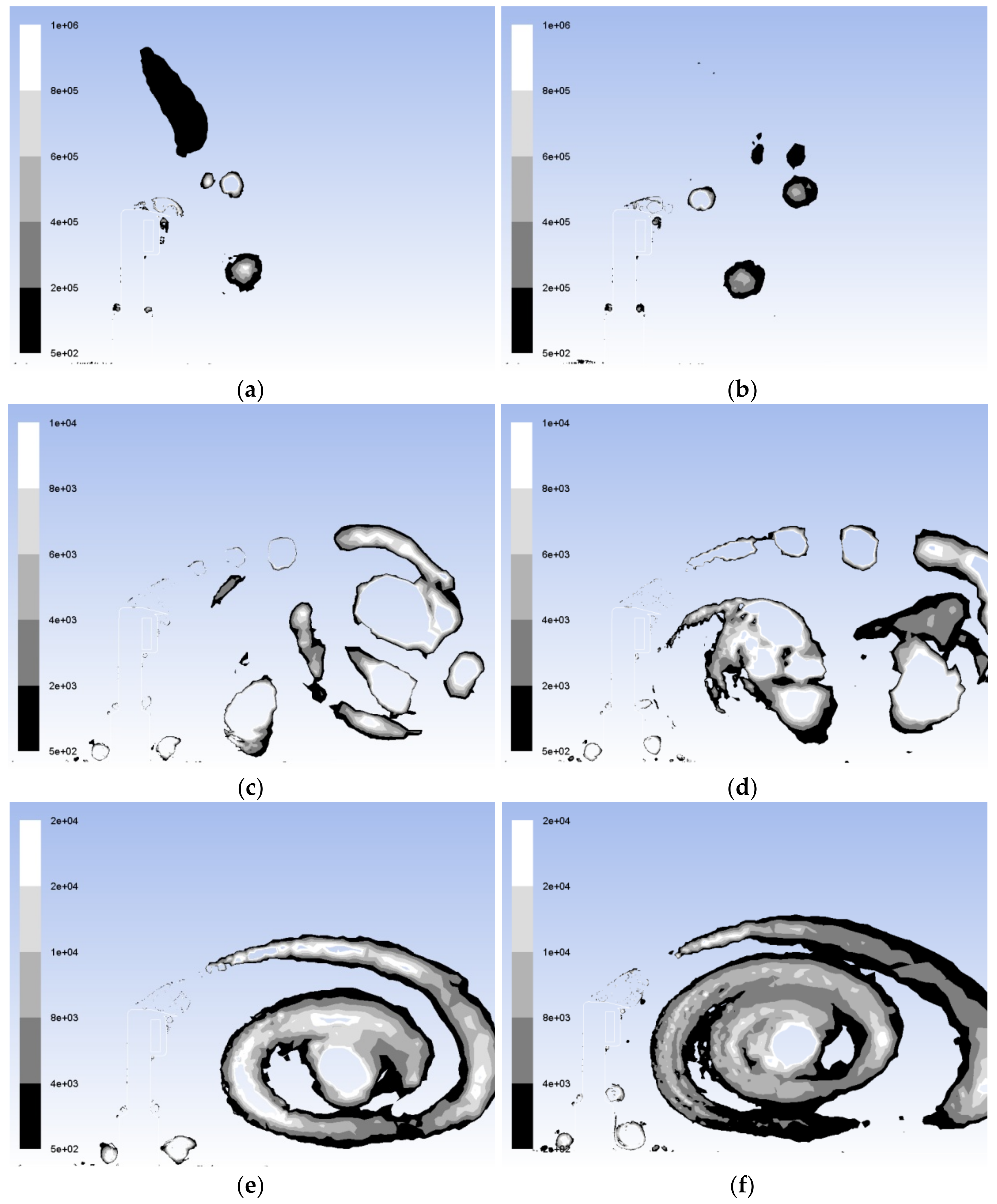
Figure 19 shows the isosurfaces obtained using the Q-Criterion applied to the velocity flow of 15 m/s. The isovalues presented in Figure 19a–f show the longitudinal vortices variation in time at the wake region of the radar without a turbulence reduction system. The dominant vortices are emphasized and clearly predicted from the beginning of the simulation. The topology of the turbulent flow field at the wake region is well solved and visualized. A vortex structure is present at the upper surface and the base of the radar body. This vortex structure persists and gains in strength at the upper surface of the radar, and is developed into the main structure at the wake region. The boundary layer over the upper surface of the radar is believed to be responsible for the vortex growth and its intensity gain. It can therefore be concluded that there are no additional main vortex structures in the wake.

7.2. Radar Mounted with a Turbulence Reduction System Flow Analysis

In this section, the wake region of the radar mounted with a proposed turbulence reduction system was analyzed. The radar surface denoted by “upper surface” in Figure 15 by number 3 is the location where the turbulence reduction system was installed; in this location, the dynamic pressure was higher, flow separation was important and eddies started to occur.

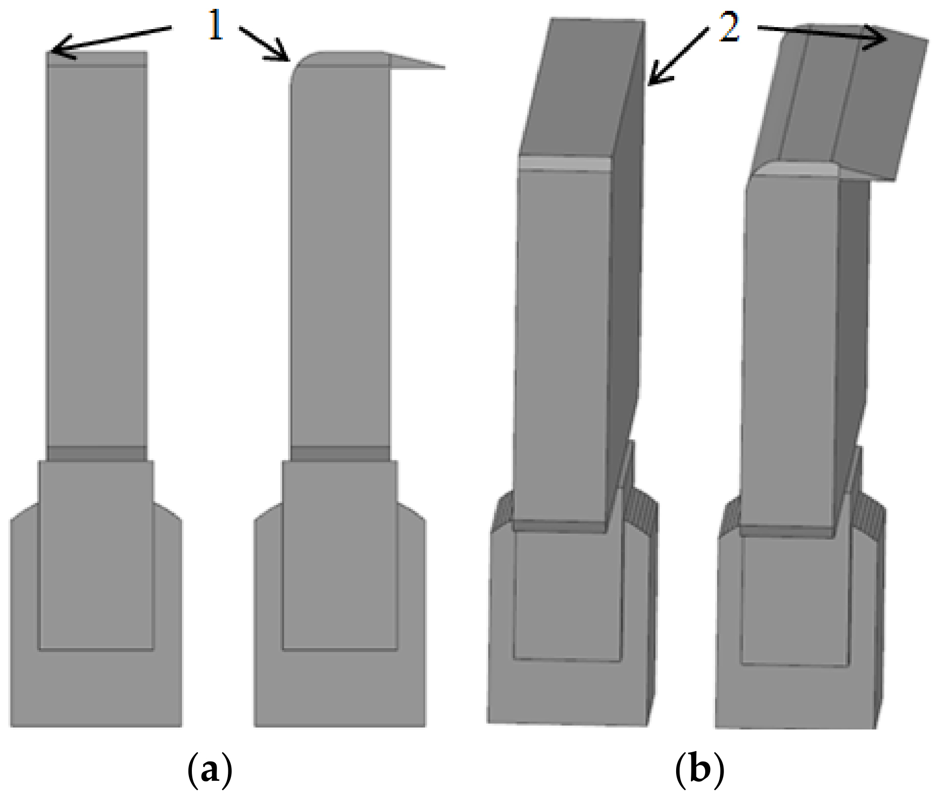
Figure 20 shows the original radar geometry (a) equipped with the proposed turbulence reduction system (b); The sharp edge was changed to a streamlined edge, as shown by number 1; at the upper rear surface of the radar, a turbulence reduction system was positioned, as shown by number 2. The system had a length of 0.50 m and was inclined with an angle of 25° at the top of the radar. The turbulence reducing system could have a high impact on the reduction of abrupt pressure gradients at the surface of the radar, and an important decrease in vortices formation downstream the wake region. The size and location of the turbulence reduction system did not affect the weight or the operating behavior of the radar.

The optimization of the curvature of the front upper surface of the radar referred to in our article by “leading edge” was considered. The optimized radius of the leading edge should be calculated by considering a compromise between the CFD simulation models (using the same metrics presented in this paper to evaluate the turbulence reduction system) and the manufacturing tolerances needed for the prototype. It is well-known that in the field of experimental testing, the numerical model predictions have to take into account the fabrication (machining) limitations (tolerances) of a prototype.

The “leading edge” optimization shape algorithm has to take into account the fabrication limitations variables (constraints) to produce a viable solution. The development of a prototype with the proposed “turbulence reduction system” and with an “optimized leading edge shape” is part of future research.

It is important in this section to find a way to compare the performance of the turbulence reduction system on the original radar shape. Figure 21 shows the streamline dynamic pressures on the radar body mounted with the turbulence reduction system, which gradually increases from low-pressure regions visualized in blue color to higher pressure regions shown in orange and red colors. The four recirculation regions shown in Figure 18 are also presented in Figure 21. The main recirculation region indicated by number 4 in Figure 21 has reduced in size to a diameter of 1.4 times the height “H” of the radar. The secondary recirculation region indicated by the number 3 reduced in size to 0.3 times the height “H” and the two separation bubbles indicated by numbers 1 and 2 were reduced in size significantly.

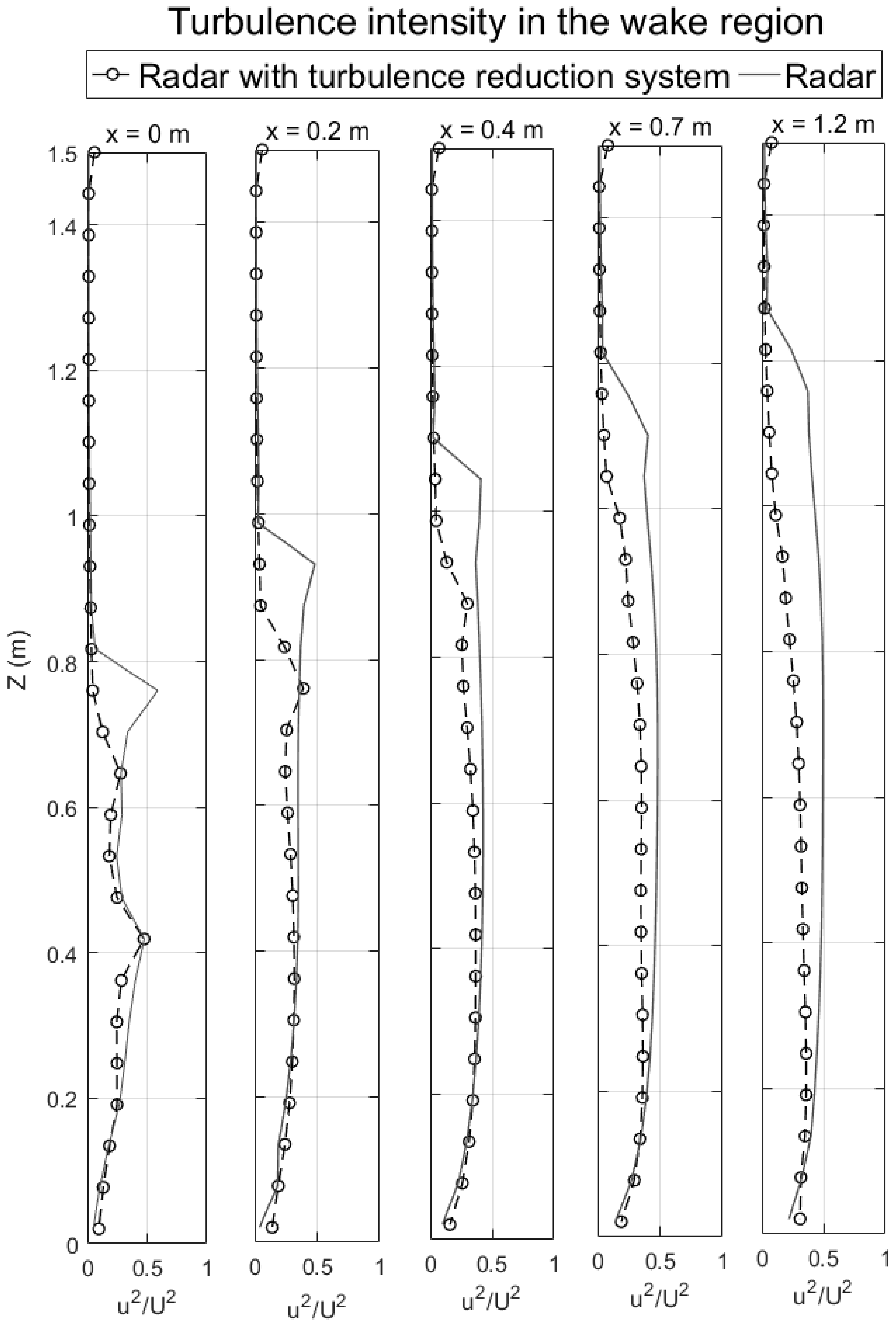
The local turbulence intensity data in five locations inside the wake region of the original radar, and of the radar with the turbulence reducing system can be seen in Figure 22. These five locations behind the radar body and along the z-axis (vertical plane) were chosen because of the high-pressure gradients and important recirculation regions obtained numerically, and are also shown in Figure 18 and Figure 22. The five locations described the flow behavior at the radar rear (x = 0 m), at 0.2 m from the radar rear (x = 0.2 m), at 0.4 m from the radar rear (x = 0.4 m), at 0.7 m from the radar rear (x = 0.7 m) and at 1.2 m from the radar rear (x = 1.2 m) were calculated. The normalized values between 0 and 1 of the turbulence intensity I were calculated at five downstream locations for the two radar models. The original radar model was represented by a “solid” line and the radar with the turbulence reduction system was shown by a “circle dash” line. A significant decrease in flow turbulence was found for the radar with a turbulence reduction system at each of the five wake locations. In Figure 22, abrupt changes in turbulence intensities seen by “peaks” in the solid lines (original radar) for all locations were considerably reduced due to a gradual evolution of the turbulent flow behavior downstream the wake, which is shown by the “circle dash” lines (radar with the turbulence reduction system). The wake regions with the highest improvement in flow conditions were located above the “upper surface” of the radar, where the turbulence reduction system was installed. These locations above the radar, at heights between z = 0.6 m and z = 1.2 m, presented a turbulence intensity reduced by half (u²/U² = 0.5).

The Q-Criterion separates very well the regions where the flow rotations are high. The Q threshold identifies the longitudinal vortices and allows one to find the main vortex structure in the wake region. The chosen upper and lower Q limits do not have any effects on the location or size of the detected vortex. The vortex structure shown in Figure 23 grows in size and strength as it spans downstream the radar body. The isovalues shown in Figure 23a–f show the longitudinal vortices variation in time and it can be noted that the vortex radius is higher when a turbulence reduction system is not installed on the radar. In the case of the radar with turbulence reduction system, the main vortex had moved closer to the reduced scale radar body. The boundary layer over the upper surface of the radar is still originated from the main vortex, but its kinetic energy is smaller than the kinetic energy needed for the vortex growth.

7.3. Metrics for Turbulent Flows

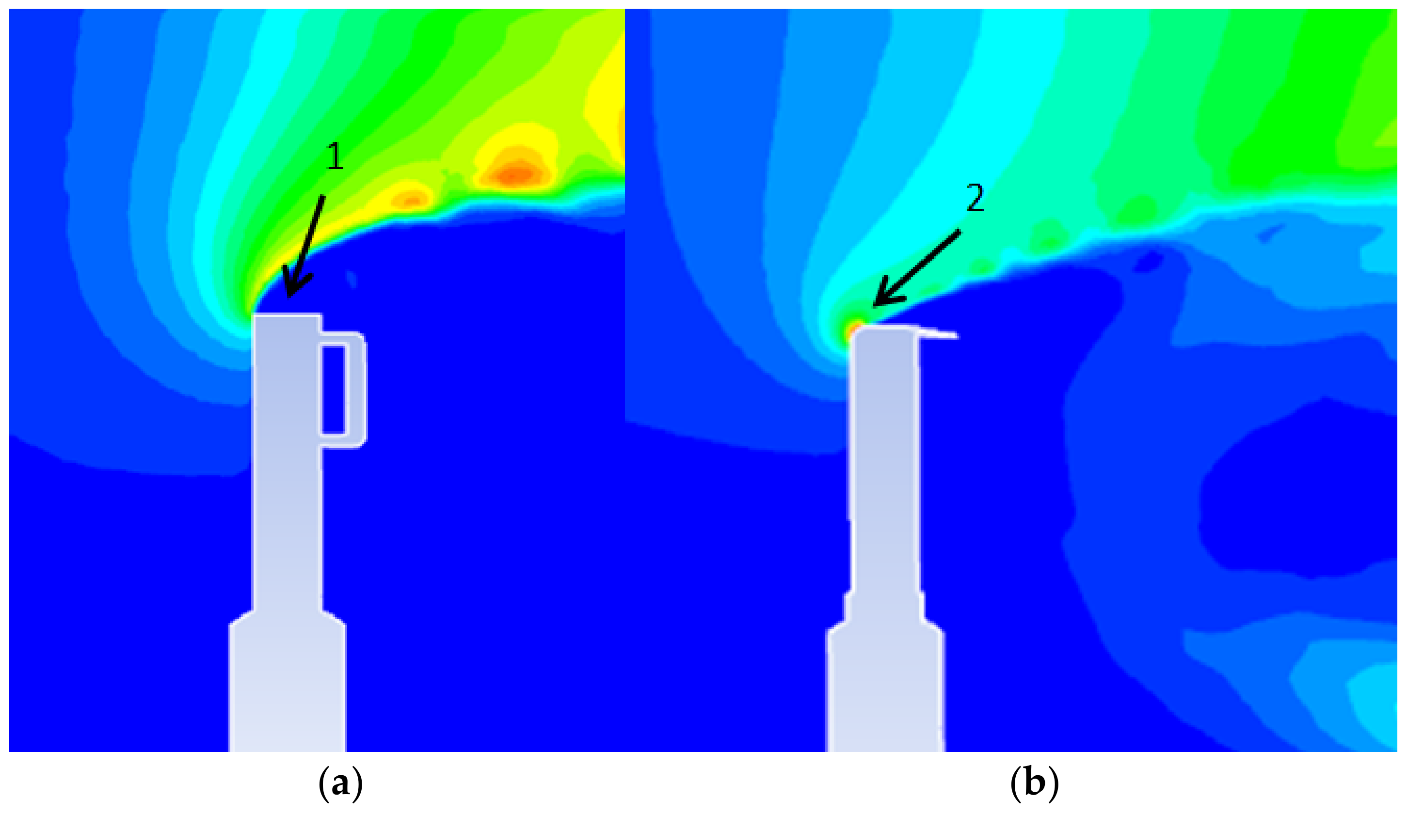
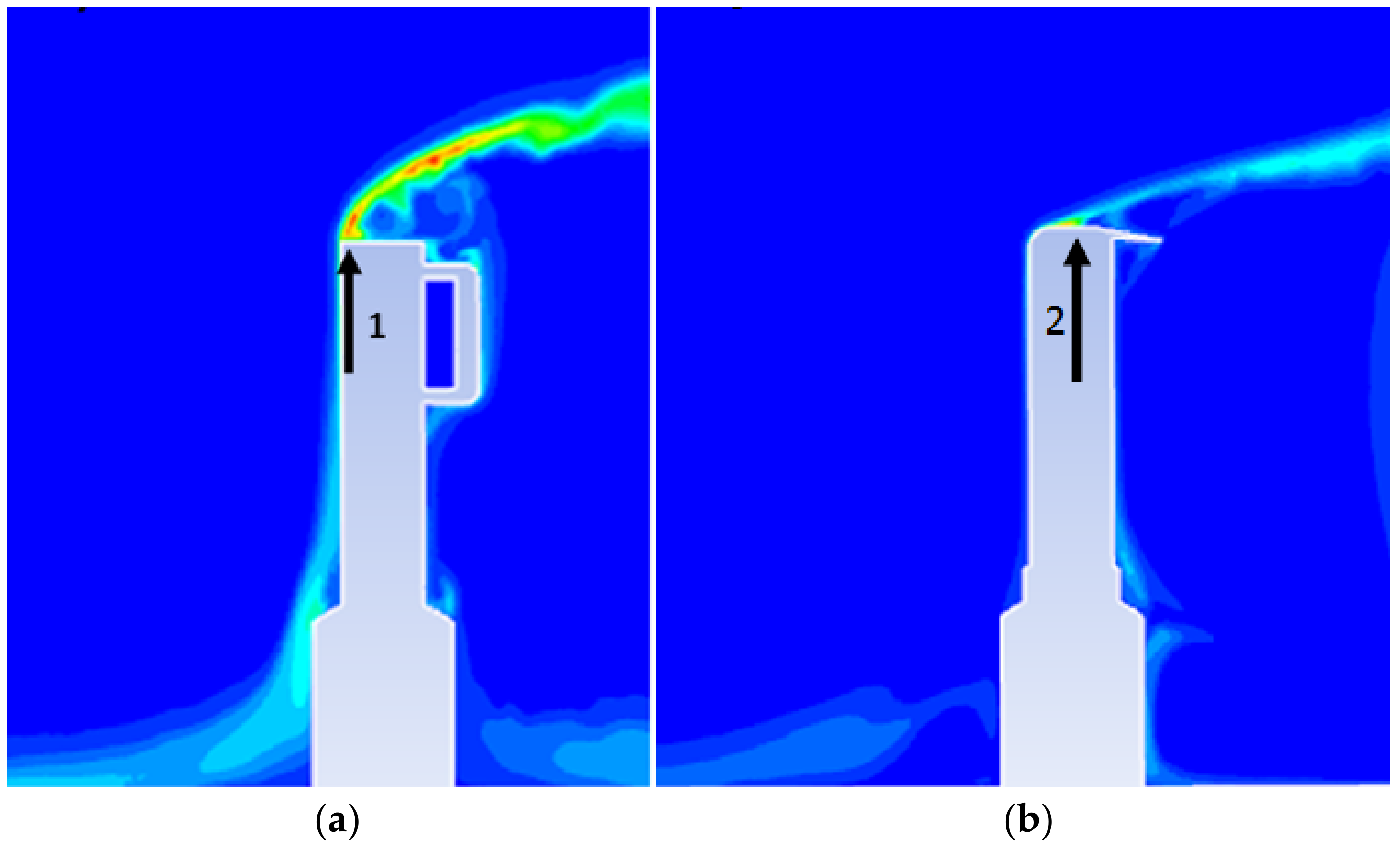
The flow differences in the wake regions of the original radar (a) and of the radar with the turbulence reduction system (b) were shown in Figure 24. The high-pressure gradients, the short transition length, the boundary layer separation, and the fully turbulent behavior at the time when the flow contacts the radar body can be seen in Figure 24a indicated by number 1. The proposed turbulence reduction system had a streamlined shape with a pre-determined flap that allowed the reduction of flow fluctuations and vortex shedding production. The improved flow behavior had also a positive impact on the turbulence intensity, the pressure distribution coefficient, the transition point, and the drag coefficient of the original radar shape. The number 2 indicated in Figure 24b presents the improved wake region of the radar with the turbulence reduction system.

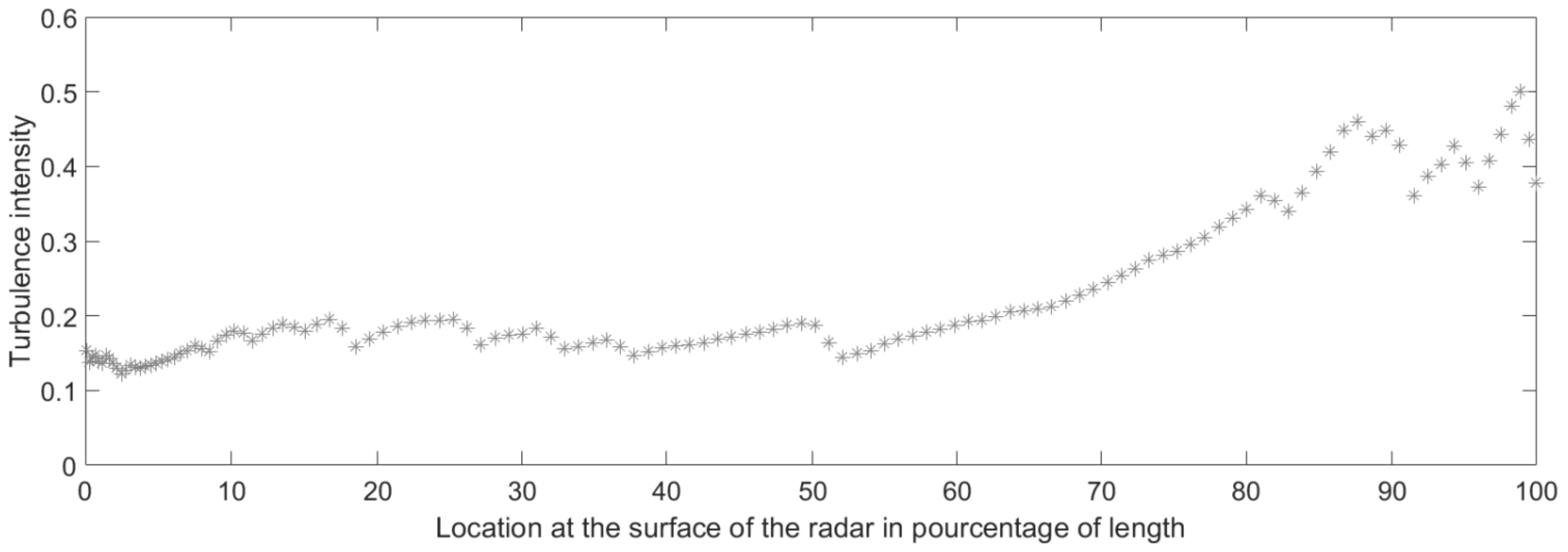
The turbulence intensity I expressed in Equation (10) was one of the parameters used to measure the performance of the turbulence reduction system. Figure 25 shows the turbulence variation at the surface of the radar called the “upper surface”. At the initial point of contact location 0% at the surface of the radar, the turbulence intensity has increased to 15%, compared to the laminar incoming flow with lower turbulence intensity (I = 0.1%). For the first half of location 0% to 50%, it can be seen that the turbulence intensity values fluctuations range from 0.15 = 15% and 0.20 = 20%. At the second half of location 50% to location 100%, the numerical model predicts higher values of turbulence, up to 0.50 = 50%, the boundary layer can no longer reattach to the surface of the radar and the flow becomes fully separated, as seen on Figure 25.

Figure 26a shows the transition point on the original radar model, as another metric parameter needed to measure the improvement of the flow at the wake region. The boundary layer separates at the location 6.5% from the leading edge of the radar, shown by number 1. After this point, a flow in the opposite direction to the free stream creates a recirculation region, which keeps the boundary layer from reattaching to the surface. The turbulence reduction system allows the boundary layer to remain attached to the surface at a longer distance. The turbulence transition point had been delayed to the location 50% = 0.50, as shown in Figure 26b by number 2. The improvement of the transition point has been also shown in the numerical data presented in Figure 25. It has been observed that the transition point has been delayed by $\frac{50\%}{6.5\%}$ = 7.6 times with the aid of the turbulence reduction system. After the location 50% = 0.50, the turbulence increased abruptly with high-intensity values, which indicates a fully detached turbulence flow.

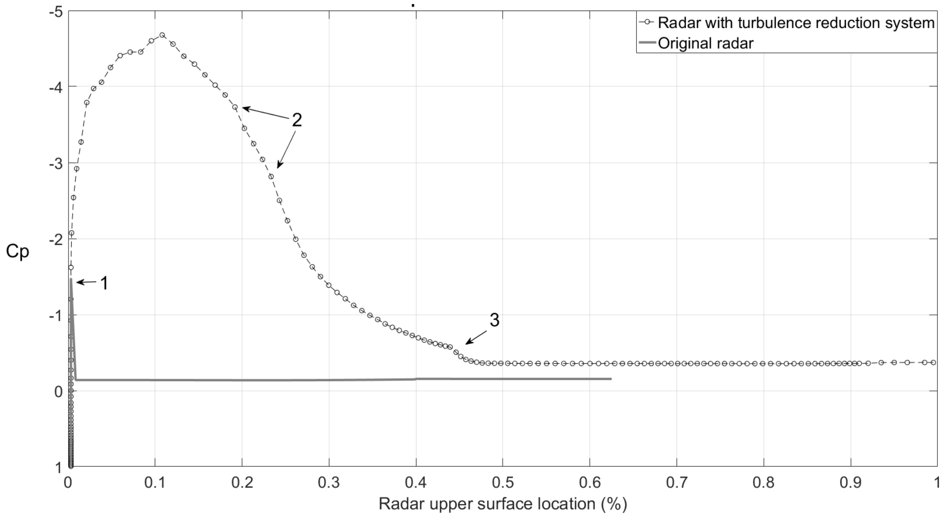
The pressure coefficient $C_p$ contributed to the evaluation of the turbulence reduction system. The dimensionless values of $C_p$, as expressed in Equation (8), can be used to determine the maximum flow speed locations and magnitudes of adverse pressure gradients, which are associated with regions of flow transition and boundary layer separation. The numerical data of pressure distributions at the surface of the original radar and the surface of the radar with the turbulence reduction system are presented in Figure 27. The pressure distribution changes abruptly from high static pressure to a low static pressure due to the radar blunt shape while the $C_p$ varies on a short distance because of the fact that the boundary layer could not develop gradually at the surface of the original radar, as indicated by the data shown in the “solid” line on Figure 27 by number 1. The “circle dash” lines on Figure 27 present pressure coefficients variation on the radar upper surface, that were obtained from the CFD model of the radar mounted with the turbulence reduction system.

A pressure gradient $C_p=-4.67$ that acts as a “suction force” of the boundary layer on the radar’s upper surface was found at the location 10.2%. This location of minimum $C_p$ also indicates the beginning of the “pressure recovery” region. After this $C_p$ value, the adverse pressure gradients keep increasing at the surface of the radar, but the high values of the local static pressure kept the boundary layer from its reattaching, as indicated by number 2 in Figure 27. The time when the boundary layer separated, and when the flow was unsteady and fully turbulent at the surface of the radar was indicated by number 3. Downstream this transition point, from location 45.5% to the trailing edge of the radar (location at 100%), the pressure coefficient was constant, $C_p=-0.3$, the boundary layer thickness was very small, the local flow was moving slowly and the turbulence intensity values were the highest.

In this section, the drag coefficient was used to measure the drag force reduction of the radar body. The flow around a blunt body separates early, resulting in adverse pressure gradients at its surface by increasing the boundary layer separation and the contribution of pressure drag or “form drag” to the total drag of the body. However, the magnitude of the pressure drag can be reduced by improving the flow conditions at the wake region and by delaying flow separation. To evaluate the turbulence reduction system in terms of drag reduction, we had to use the experimental data collected for the original radar body, as presented in Figure 6. The angular position of zero degrees for the radar body and a flow Reynolds number of 4 × 10⁵ was chosen because of the fact that these conditions are the most demanding and challenging operating conditions for the radar presented in this study. The drag coefficient for the original radar was C_d = 3.51 while C_d = 3.17 for the radar mounted with the turbulence reduction system.

The high effectiveness of the turbulence reduction system led to the turbulence intensity reduction at the surface of the radar, the flow transition delay, while the transition point moved downstream the surface of the radar and increased the boundary layer “suction force”; thus, major positive impacts were observed in the “form drag” produced by the blunt body. It is concluded that the turbulence reduction system has decreased the drag coefficient of the original radar by a percentage of $\frac{3.17-3.51}{3.51}=-9.67\%$.

8. Conclusions

The new methodology proposed in this paper allowed a detailed investigation of the wake region of the original radar body and the radar body with a turbulence reduction system. The numerical results obtained on the original radar’s wake region showed periodic vortex shedding, boundary layer separation, high levels of turbulence, and induced drag; The nature of the adverse pressure gradient and high turbulence intensity values at the radar surface needed a mechanism to reduce flow fluctuation and to allow the boundary layer to increase.

This study showed also the results of the Price-Païdoussis wind tunnel experiments for a large “ground surveillance radar”. The wind tunnel test data completed, and thus validated the numerical results obtained for the Strouhal number, Reynolds number, and drag coefficients values. Spectral analysis was also performed on the experimental data. The forces and moments data showed high dependency on the angular position of the radar and low dependency on the wind tunnel flow speed. Vortex shedding tended to occur at any angular position at different shedding frequencies. Based on experimental values, one shedding frequency and one high drag coefficient were obtained at Reynolds number 4 × 10⁵ and when the radar was perpendicular to the flow. It was decided to measure the performance of the proposed “turbulence reduction system” for the same flow conditions.

The flow pattern at the wake region was identified in the absence of distorting effects of direct measurements using probes and visualization methods, such as “white smoke” and “tufts” attached to a wing model surface. It was demonstrated that a turbulence reduction system mounted on the radar surface can improve its behavior at all flow conditions. The CFD model was an important tool to understand and analyze the flow around the radar because of the fact that it indicated the regions where flow separated and then reattached; in these regions of stagnation and recirculation, eddies and vortices were formed. Using the CFD model data, a turbulence reduction system with an optimized upper profile and a streamlined flap surface was proposed.

Based on the CFD model results, it was concluded that the adverse pressure gradients have significantly decreased at the upper surface of the radar with its turbulence reduction system mounted. The proposed system strongly influenced the unsteady flow fluctuations and vortex shedding as the large turbulent motions were suppressed in the wake region. The numerical results showed an important reduction of the turbulence intensity as well as a growth in the boundary layer region compared to that of the original radar configuration. The pressure distribution developed by the proposed system helped the boundary layer to reattach to it. The turbulence reduction system produced a reduced recirculation region at the rear of the radar’s surface, due to a better control of the incoming flow.

As future work, the authors believe that the methodology proposed in this research will be useful to study and quantify unsteady flow regimes where experimental measurements of the flow are limited or difficult to obtain. A very good experiment would be able to describe and analyze the flow near a self-oscillating flexible membrane placed in a laminar flow; the proposed new method for flow analysis could evaluate if the vortices generated at the wake are contributing to the flapping oscillation of the membrane.

It would be also interesting to design an adaptive turbulence reduction system that will use a brushless motor to change its upper surface position. The research will also include a CFD analysis to measure the reduction of the drag coefficient, the flow transition delay, and the turbulence intensity reduction for different radar upper surface shapes and angle of attack.

References

- Lee, Y.; Rho, J.; Kim, K.H.; Lee, N.-H. Fundamental studies on free stream acceleration effect on drag force in bluff bodies. J. Mech. Sci. Technol. 2011, 25, 695–701. [Google Scholar] [CrossRef]
- Degani, A.T.; Walker, J.D.A.; Smith, F.T. Unsteady separation past moving surfaces. J. Fluid Mech. 1998, 375, 1–38. [Google Scholar] [CrossRef] [Green Version]
- Brahimi, M.T.; Paraschivoiu, I.D. Darrieus Rotor Aerodynamics in Turbulent Wind. ASME J. Sol. Energy Eng. 1995, 117, 128–136. [Google Scholar] [CrossRef]
- Mason, W.T.; Beebe, P.S. The Drag Related Flow Field Characteristics of Trucks and Buses. In Aerodynamic Drag Mechanisms of Bluff Bodies and Road Vehicles; Springer: Boston, MA, USA, 1978; pp. 45–93. [Google Scholar]
- Grigorie, L.T.; Botez, R.M.; Popov, A.V. How the Airfoil Shape of a Morphing Wing is Actuated and Controlled in a Smart Way. J. Aircr. Eng. ASCE Ed. 2015, 28, 04014043. [Google Scholar] [CrossRef]
- Sugar Gabor, O.; Koreanschi, A.; Botez, R.M.; Mamou, M.; Mébarki, Y. Numerical Simulation and Wind Tunnel Tests Investigation and Validation of a Morphing Wing-Tip Demonstrator Aerodynamic Performance. Aerosp. Sci. Technol. 2016, 53, 136–153. [Google Scholar] [CrossRef] [Green Version]
- Koreanschi, A.; Sugar Gabor, O.; Botez, R.M. Drag Optimization of a Wing Equipped with a Morphing Upper Surface. Aeronaut. J. 2016, 120, 473–493. [Google Scholar] [CrossRef]
- Sugar Gabor, O.; Koreanschi, A.; Botez, R.M. Optimization of an Unmanned Aerial System Wing Using a Flexible Skin Morphing Wing. SAE Int. J. Aerosp. 2013, 6, 115–121. [Google Scholar] [CrossRef]
- Sugar Gabor, O.; Simon, A.; Koreanschi, A.; Botez, R.M. Improving the UAS-S4 Éhecatl airfoil high angle of attack performance characteristics using a morphing wing approach. Proc. Inst. Mech. Eng. Part G J. Aerosp. Eng. 2016, 23, 118–131. [Google Scholar] [CrossRef] [Green Version]
- Tchatchueng Kammegne, M.J.; Grigorie, L.T.; Botez, R.M.; Koreanschi, A. Design and Wind Tunnel Experimental Validation of a Controlled New Rotary Actuation System for a Morphing Wing Application. Proc. Inst. Mech. Eng. Part G J. Aerosp. Eng. 2016, 230, 132–145. [Google Scholar] [CrossRef]
- Sugar Gabor, O.; Simon, A.; Koreanschi, A.; Botez, R.M. Application of a Morphing Wing Technology on Hydra Technologies Unmanned Aerial System UAS-S4. In Proceedings of the ASME 2014 International Mechanical Engineering Congress and Exposition, Montreal, QC, Canada, 14–20 November 2014; Volume 1. [Google Scholar]
- Koreanschi, A.; Sugar-Gabor, O.; Botez, R.M. Numerical and Experimental Validation of a Morphed Wing Geometry Using Price-Païdoussis Wind Tunnel Testing. Aeronaut. J. 2016, 120, 757–795. [Google Scholar] [CrossRef]
- Sugar Gabor, O.; Koreanschi, A.; Botez, R.M. Analysis of UAS-S4 Éhecatl aerodynamic performance improvement using several configurations of a morphing wing technology. Aeronaut. J. 2016, 120, 1337–1364. [Google Scholar] [CrossRef]
- Rebuffet, P. Aérodynamique Expérimentale, 1st ed.; Paris Dunod: Paris, France, 1996; p. 566. [Google Scholar]
- Duell, E.G.; George, A.R. Measurements in the Unsteady Near Wakes of Ground Vehicle Bodies; SAE Technical Paper; SAE International: Warrendale, PA, USA, 1993. [Google Scholar]
- Roshko, A. On the Drag and Shedding Frequency of Two-Dimensional Bluff Bodies; Technical Note; National Advisory Committee for Aeronautics: Washington, DC, USA, 1954.
- Menter, F.R.; Kuntz, M. Adaptation of Eddy-Viscosity Turbulence Models to Unsteady Separated Flow Behind Vehicles. In The Aerodynamics of Heavy Vehicles: Trucks, Buses and Trains; Springer: Berlin/Heidelberg, Germany, 2004. [Google Scholar]
- Cestino, E.; Frulla, G.; Spina, M.; Catelani, D.; Linari, M. Numerical Simulation and experimental validation of slender wings flutter behavior. J. Aerosp. Eng. 2019, 233, 5913–5928. [Google Scholar]
- Kalitzin, G.; Medic, G.; Iaccarino, G.; Durbin, P. Near-wall Behaviour of RANS Turbulence Models and Implications for Wall Functions. J. Comput. Phys. 2005, 204, 265–291. [Google Scholar] [CrossRef]
- Durbin, P.A. Separated Flow Computations with the k-e-v2 Model. AIAA J. 1995, 33, 659–664. [Google Scholar] [CrossRef]
- Frunzulică, F.; Dumitrescu, H.; Dumitrache, A. A numerical investigation on the dynamic stall of a vertical axis wind turbine. Proc. Appl. Math. Mech. 2013, 13, 295–296. [Google Scholar] [CrossRef]
- Fröhlich, J.; von Terzi, D. Hybrid LES/RANS Methods for Simulation of Turbulent Flows. Prog. Aerosp. Sci. 2008, 44, 349–377. [Google Scholar] [CrossRef]
- ASME. Guide for Verification and Validation in Computational Solid Mechanics; Release 10; The American Society of Mechanical Engineers: New York, NY, USA, 2016. [Google Scholar]
- Ferson, S.; Oberkampf, W.; Ginzburg, L. Model validation and predictive capability for the thermal challenge problem. Comput. Methods Appl. Mech. Eng. 2008, 197, 29–32. [Google Scholar] [CrossRef]
- Brahimi, M.T.; Allet, A.; Paraschivoiu, I. Aerodynamic Analysis Models for Vertical-Axis Wind Turbines. Int. J. Rotating Mach. 1995, 2, 15–21. [Google Scholar] [CrossRef]
- Romeo, G.; Cestino, E.; Pacino, M.; Borello, F.; Correa, G. Design and testing of a propeller for a two-seater aircraft powered by fuel cells. Proc. Inst. Mech. Eng. Part G J. Aerosp. Eng. 2012, 226, 804–816. [Google Scholar] [CrossRef]
- Correa, G.; Santarelli, M.; Borello, F.; Cestino, E.; Romeo, G. Flight test validation of the dynamic model of a fuel cell system for ultra-light aircraft. J. Aerosp. Eng. 2015, 229, 917–932. [Google Scholar] [CrossRef]
- Dubief, Y.; Delcayre, F. Coherent-vortex identification in turbulence. J. Turbul. 2000, 1, 011. [Google Scholar] [CrossRef]
- Jeong, J.; Hussain, F. On the identification of a vortex. J. Fluid Mech. 1995, 285, 69–94. [Google Scholar] [CrossRef]
- Hunt, J.C.R.; Wray, A.A.; Moin, P. Eddies, Stream and Convergence Zones in Turbulent Flows; Summer Program of the Center for Turbulence Research, NASA Ames/Stanford University: Stanford, CA, USA, 1988; pp. 193–207. [Google Scholar]
- Mariotti, A.; Buresti, G.; Salvetti, M.V. Separation delay through contoured transverse grooves on a 2D boat-tailed bluff body: Effects on drag reduction and wake flow features. Eur. J. Mech. B Fluids 2019, 74, 351–362. [Google Scholar] [CrossRef]
- Rocchio, B.; Mariotti, A.; Salvetti, M.V. Flow around a 5:1 rectangular cylinder: Effects of upstream-edge rounding. J. Wind Eng. Ind. Aerodyn. 2020, 204, 104237. [Google Scholar] [CrossRef]
- Maskell, E.C. A Theory of the Blockage Effect on Bluff Bodies and Stalled Wings in a Closed Wind Tunnel; ARC R&M 3400; Aeronautical Research Council London: London, UK, 1968.
- FLIR Inc. Available online: https://www.flir.ca/support/products/ranger-r20ss/ (accessed on 11 January 2021).
- Martin, S. PC-based data acquisition in an industrial environment. In Proceedings of the IEE Colloquium on PC-Based Instrumentation, London, UK, 31 January 1990. [Google Scholar]
- Barlow, J.B.; Rae, W.H.; Pope, A. Low-Speed Wind Tunnel Testing, 3rd ed.; John Wiley & Sons: New York, NY, USA, 1999. [Google Scholar]
- Garner, H.C.; Rogers, E.; Acum, W.; Maskell, E.C. Subsonic Wind Tunnel Wall Correction; National Physical Laboratory: Teddington, UK, 1966. [Google Scholar]
- Eisenlohr, H.; Eckelmann, H. Vortex Splitting and its Consequences in the Vortex Street Wake of Cylinders at Low Reynolds Number. Phys. Fluids 1989, 1, 189–192. [Google Scholar] [CrossRef]
- Katz, A.; Sankaran, V. Mesh quality effects on the accuracy of CFD solutions on unstructured meshes. J. Comput. Phys. 2011, 230, 7670–7686. [Google Scholar] [CrossRef]
- Bradshaw, P. Understanding and predictions of turbulent flow. Int. J. Heat Fluid Flow 1997, 18, 45–54. [Google Scholar] [CrossRef]
- Spalart, P. Strategies for turbulence modelling and simulations. Int. J. Heat Fluid Flow 2000, 21, 252–263. [Google Scholar] [CrossRef]
- Menter, F. Review of the shear-stress transport turbulence model experience from an industrial perspective. Int. J. Comput. Fluid Dyn. 2009, 23, 305–316. [Google Scholar] [CrossRef]
- Kroll, N.; Rossow, C.C.; Schwamborn, D.; Becker, K.; Heller, G. A Numerical Flow Simulation Tool for Transport Aircraft Design. In Proceedings of the 23rd ICAS Congress, Toronto, ON, Canada, 8–13 September 2002. [Google Scholar]
- Jameson, A.; Pierce, M.; Martinelli, L.; Pierce, N.A. Optimum Aerodynamic Design using Navier-Stokes Equations. Theoret. Comput. Fluid Dyn. 1998, 10, 213–237. [Google Scholar] [CrossRef] [Green Version]
- Fluent User’s Manual. Available online: https://www.sharcnet.ca/Software/Ansys/17.0/en-us/help/flu_ug/flu_ug.html (accessed on 9 February 2021).
- Chatenet, Q.; Tahan, A.; Gagnon, M.; Chamberland-Lauzon, J. Numerical model validation using experimental data: Application of the area metric on a Francis runner. In Proceedings of the 28th IAHR Symposium on Hydraulic Machinery and Systems, Grenoble, France, 4–8 July 2016. [Google Scholar]
Figure 1.
Flow behavior at the wake on a blunt body, a figure designed by the author.
Figure 2.
Price-Païdoussis Blow Down Subsonic Wind Tunnel.
Figure 3.
Price-Païdoussis Wind Tunnel schematic designed by authors.
Figure 4.
Front and rear images of the full-size radar.
Figure 5.
Experimental drag forces at various angular positions.
Figure 6.
Experimental drag coefficients versus yaw angle and Reynolds numbers.
Figure 7.
Time history of drag coefficients for angular position 0°.
Figure 8.
Power spectrum frequencies on the radar drag coefficients.
Figure 9.
Mesh resolution of the radar model.
Figure 10.
Representation of the radar inside the wind tunnel test section for the numerical CFD model.
Figure 11.
Area Metric results for Fx.
Figure 12.
Area Metric results for Fy.
Figure 13.
Area Metric results for Mx.
Figure 14.
Area Metric results for My.
Figure 15.
Flow interaction locations on the radar surface.
Figure 16.
Simulation results of dynamic pressure at the wake region.
Figure 17.
Simulation results of turbulence intensity I at the wake region.
Figure 18.
Streamlines simulation of the dynamic pressure (Pa) for the original radar.
Figure 19.
In plane Q-Criterion simulation results of vortices variation with time (a–f) on the original radar body for Q = [101 − 106].
Figure 20.
Original radar geometry versus modified radar geometry with turbulence reduction system with side view (a) and upper view (b).
Figure 21.
Streamlines simulation of the dynamic pressure (Pa) for the radar with turbulence reduction system.
Figure 22.
Turbulence intensity at five wake locations of the original radar and the radar with the turbulence reduction system.
Figure 23.
In plane Q-Criterion simulation results of vortices variation with time (a–f) of the flow near the radar with a turbulence reduction system for Q = [101 − 106].
Figure 24.
Pressure gradients simulation on the original radar (a) and for the radar with turbulence reduction system (b).
Figure 25.
Turbulence intensity at the upper surface of the radar with turbulence reduction system.
Figure 26.
Transition point location simulation on the original radar (a) versus the radar with turbulence reduction system (b).
Figure 27.
Pressure coefficients on the upper surface of the radar.
Publisher’s Note: MDPI stays neutral with regard to jurisdictional claims in published maps and institutional affiliations. |
© 2021 by the authors. Licensee MDPI, Basel, Switzerland. This article is an open access article distributed under the terms and conditions of the Creative Commons Attribution (CC BY) license (https://creativecommons.org/licenses/by/4.0/).
Share and Cite
MDPI and ACS Style
Salinas, M.F.; Botez, R.M.; Gauthier, G. New Numerical and Measurements Flow Analyses Near Radars. Appl. Mech. 2021, 2, 303-330. https://0-doi-org.brum.beds.ac.uk/10.3390/applmech2020019
AMA Style
Salinas MF, Botez RM, Gauthier G. New Numerical and Measurements Flow Analyses Near Radars. Applied Mechanics. 2021; 2(2):303-330. https://0-doi-org.brum.beds.ac.uk/10.3390/applmech2020019
Chicago/Turabian StyleSalinas, Manuel Flores, Ruxandra Mihaela Botez, and Guy Gauthier. 2021. "New Numerical and Measurements Flow Analyses Near Radars" Applied Mechanics 2, no. 2: 303-330. https://0-doi-org.brum.beds.ac.uk/10.3390/applmech2020019