Numerical and Experimental Study of Aerodynamic Performances of a Morphing Micro Air Vehicle


1
Instituto Nacional de Técnica Aeroespacial (INTA), Torrejón de Ardoz, 28850 Madrid, Spain
2
Department of Aircraft and Space Vehicles at Escuela Técnica Superior de Ingeniería Aeronáutica y Espacio (ETSIAE), Universidad Politécnica de Madrid (UPM), 28040 Madrid, Spain
*
Author to whom correspondence should be addressed.
Appl. Mech. 2021, 2(3), 442-459; https://0-doi-org.brum.beds.ac.uk/10.3390/applmech2030025
Submission received: 4 June 2021
/
Revised: 25 June 2021
/
Accepted: 2 July 2021
/
Published: 8 July 2021
Abstract
:The present work is focused on the investigation of the aerodynamic performances of a novedous bioinspired morphing Micro Air Vehicle (MAV) with an adaptive wing structure geometry. For this purpose, a numerical study of Computational Fluid Dynamics (CFD) implemented by Ansys Fluent 15.0 was performed in order to obtain insight about the aerodynamic effect of wing structure deformation when morphing devices are used, and its influence on the global aerodynamic parameters related with aircraft performances. On the other hand, an experimental study using the Particle Image Velocimetry technique and balance measurements in a Low-Speed Wind Tunnel was conducted to obtain experimental information about performances measured to establish a comparison between both, experimental and numerical results. The Micro Air Vehicle (MAV) presents a Zimmerman wing with an Eppler 61 airfoil. Three different wing configurations according to curvature and thickness variations and for all angles of attack have been studied. A comparative analysis based on aerodynamic features is performed by an assessment of lift coefficient (CL), total aerodynamic drag coefficient (CD) and aerodynamic efficiency as lift/drag ratio (CL/CD) in order to conclude the best wing configuration in terms of aerodynamic performance.
1. Introduction
In recent years, the development of bioinspired Micro Aerial Vehicles (MAVs) has become one of the biggest challenges in the aerospace industry. Many engineers and researchers around the world are designing prototypes based on non-conventional geometries and propulsion systems focused on nature to develop multiple unmanned applications. These MAVs are able to perform activities from simply commercial applications to strategic areas of defense, flying in unhealthy environments, dangerous missions or inaccessible areas. The primary objective of these type of vehicles is to avoid human accidents. The greatest features of MAVs are the small dimension (their size is approximately less than 500 mm [1]), small wingspan giving rise to a low aspect ratio (AR) and low range operation due to the low Reynolds (Re) numbers range between , besides their low-cost manufacturing due to their small dimensions.
Several developments of MAVs have been carried out over the last years. To quote briefly, Moschetta [2] developed a study based on a fixed wing, biplane, coaxial and tilt-body concept. Later, a deeply experimental testing of several wing planforms was carried out by Marek [3]. The highest lift coefficients were obtained with the Zimmerman and elliptical wing planform. Taking into account these results, a fixed wing model based on the Zimmerman wing was designed and developed by Hassanalian and Abdelkefi in Ref. [4]. This same planform was selected for developing the Dragonfly micro aerial vehicle of Flake and Stanford in Refs. [5,6].
The bioinspiration concept based on the adaptive wing structure geometry (morphing geometry) arose a bit late [7,8]. This approach focuses on varying the wing geometry in order to maximize the aerodynamic efficiency. There are several approaches to achieve this deformation: firstly, there is the planform deformation (sweep angle, wingspan or chord length can be modified); secondly, there is the out-of-plane transformation (in this case the wing twisting or chord-wise bending would be modified); finally, there is the airfoil profile adjustment (camber). Our objective is focused on the last one. The present MAV was designed based on modifying the curvature and thickness of the wing. The preliminary design of this MAV with the Zimmerman wing was published by Barcala in Ref. [9]. The lift coefficient increased with the maximum airfoil camber-to-chord ratio was studied in Ref. [10]. In this context, flying at low velocity with high lift would make recording video in real time possible with high quality, which would be very useful for many applications. The wing deformations of this vehicle have been studied by applying piezoelectric actuators inside the wing (a type of smart material) [11]. Barcala et al. [12] studied these modifications in 2018. Piezoelectric actuators are a piezoceramic material, a type of smart material whose length is modified depending on the voltage applied, that produces modifications of the wing curvature inside the wing. This MAV is based on Eppler 61 airfoils and a Zimmerman plantform. The voltage applied is from 0 V, where the wing maintains its initial dimensions (without any deformation) to 5 V, where the wing reaches its maximum deformation, both in curvature and thickness. From these results, we obtained a wing deformation in curvature and thickness while the dimensions of chord and wingspan were maintained as the beginning of the experimental testing.
This work is focused on studying a bioinspired MAV based on adaptive wing structure geometry (morphing geometry) in three wing configurations: morphing 0 V (without wing deformation), morphing 2.8 V (wing semi-deformation) and morphing 5 V (maximum deformation of the wing). The MAV was designed by the CATIA V5 software and manufactured by 3D printing with Polylactic Acid (PLA). As the ultimate goal of this paper is to improve the aerodynamic performance of this MAV, a complete analysis of, both, experimental and numerical and for all angles of attack. The experimental campaign was carried out in a Low-Speed Wind Tunnel and fluid flow field numerical simulations were developed by using Ansys Fluent 2020 at Instituto Nacional de Técnica Aeroespacial (INTA).
2. Theoretical Background
In this section, a previous theoretical background of the aerodynamic performance in aircraft is presented. The wake survey analysis will be performed to determine the lift () and induced drag coefficients, while the total aerodynamic coefficient will be obtained by means of a balance.
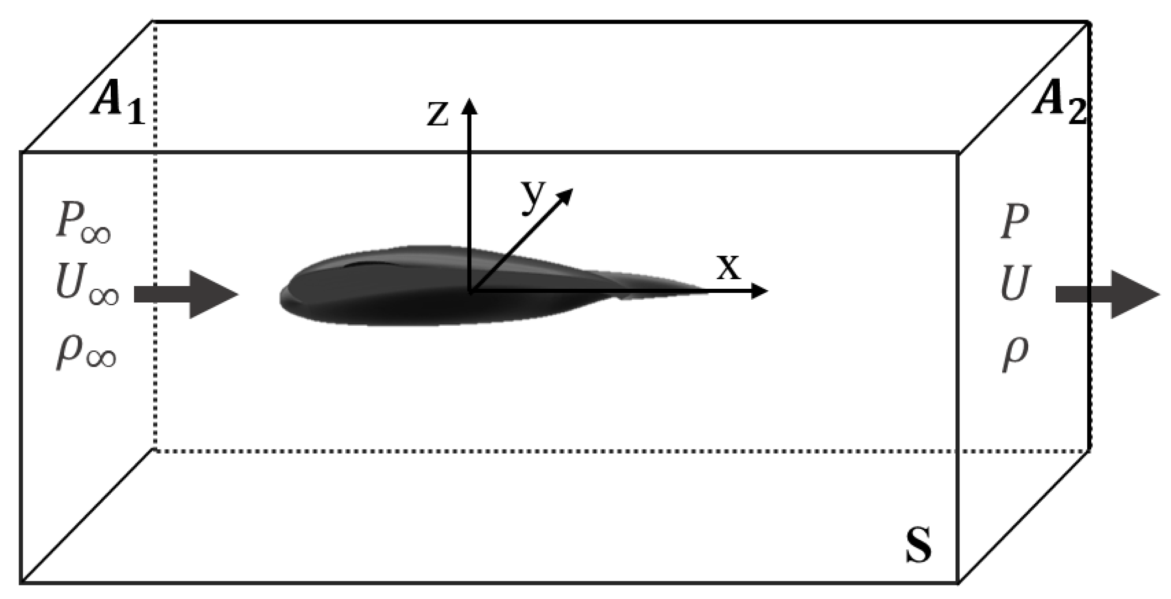
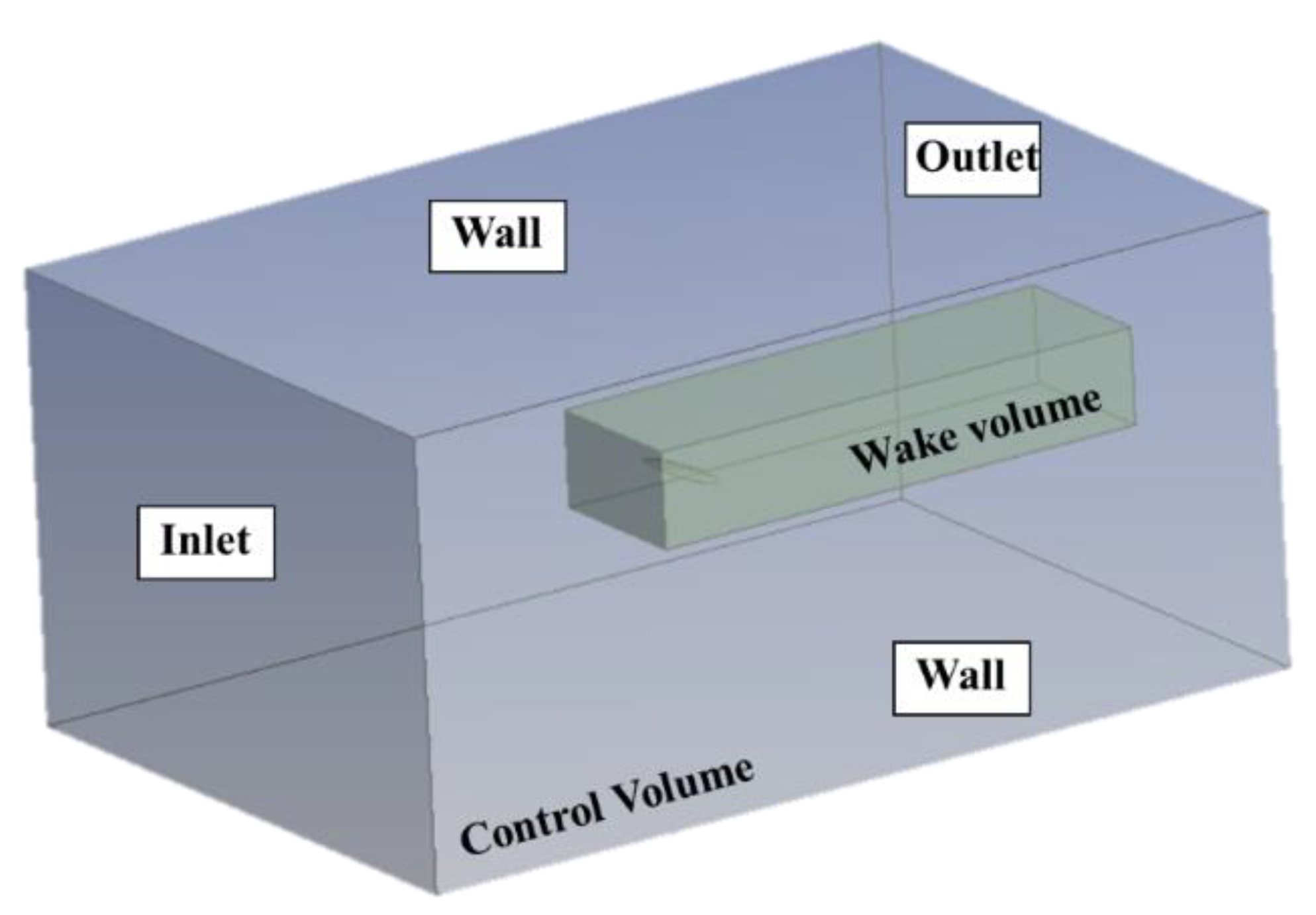
The wake survey analysis is based on obtaining the pressure and velocity components in a plane located in the wake far away from the trailing edge of the model (Trefftz Plane). The following Figure 1 shows the fluid control volume required to perform the experimental and numerical analysis of this MAV.
To determine the total aerodynamic drag and lift forces based on the wake survey analysis, the four following assumptions are required [13]:
- (1)
- The fluid flow measurements have to be performed in a transversal and downstream section to the MAV, plane A2 in Figure 1 (this plane is perpendicular to the X-axis, wind tunnel axis).
- (2)
- The flow in plane A2 is steady and incompressible.
- (3)
- The flow inside the fluid control volume without the MAV behaves as a uniform freestream parallel to the X-axis (wind tunnel axis) and its velocity is tangent to the walls (all surface of S (control volume) except to A1 and A2).
- (4)
- Fluid viscous stress terms are neglected in section A2 due to the distance of this plane is far away from the trailing edge of the MAV.
Taking into account these assumptions, the lift L (Equation (1)) and total aerodynamic drag D (Equation (2)) forces acting on the MAV are evaluated by applying the fluid momentum equations to the control volume of Figure 1:
where is the local density, is the velocity vector (), is the normal vector to the outward surface, and is the freestream static pressure.
Betz, Maskell and Kupunas developed a theory [14,15,16,17] based on integrating the total pressure loss in a line contained in a downstream plane (a plane inside A2 but only encompassing the wake of the model, wake plane ()) to the model resulting in two-dimensional drag. Therefore, by applying this theory, the lift and total aerodynamic drag forces correspond to the Equations (3) and (4), respectively:
where is the axial vorticity of the fluid, the gas constant, the freestream velocity, P the local pressure, s the entropy, the ratio of specific heats, the freestream Mach number, the freestream density, and , and the velocities in and directions, respectively.
The total aerodynamic drag force, the first term of Equation (4) corresponds to the ‘parasitic drag, ’, the second term is the “induced drag, ” and the third term corresponds to a second-order correction of the which could be neglected according to Ref. [18]. In the present work, the third integral was neglected since the flow is incompressible. Consequently, the final total aerodynamic drag results as the sum of parasitic and induced drag components.
Regarding the lift force, as the flow is incompressible, the only term required to obtain this force is the first integral of Equation (3), since the other integrals are neglected. The final lift force equation is:
By dividing the Equations (5) and (6) (total aerodynamic drag and lift, respectively) into , the aerodynamic coefficients are obtained. is the dynamic pressure and the wing surface of the reference. Equations (7)–(9) correspond to the parasitic drag coefficient,, induced drag coefficient, and lift coefficient, respectively:
3. MAV with an Adaptative Wing Geometry
MAV Model
The present paper is focused on a MAV with an adaptive wing structure geometry. This model presents a low wing aspect ratio (AR = 2.5) and low operating range (low Reynolds number). The features of the studied MAV are shown in the following Table 1:
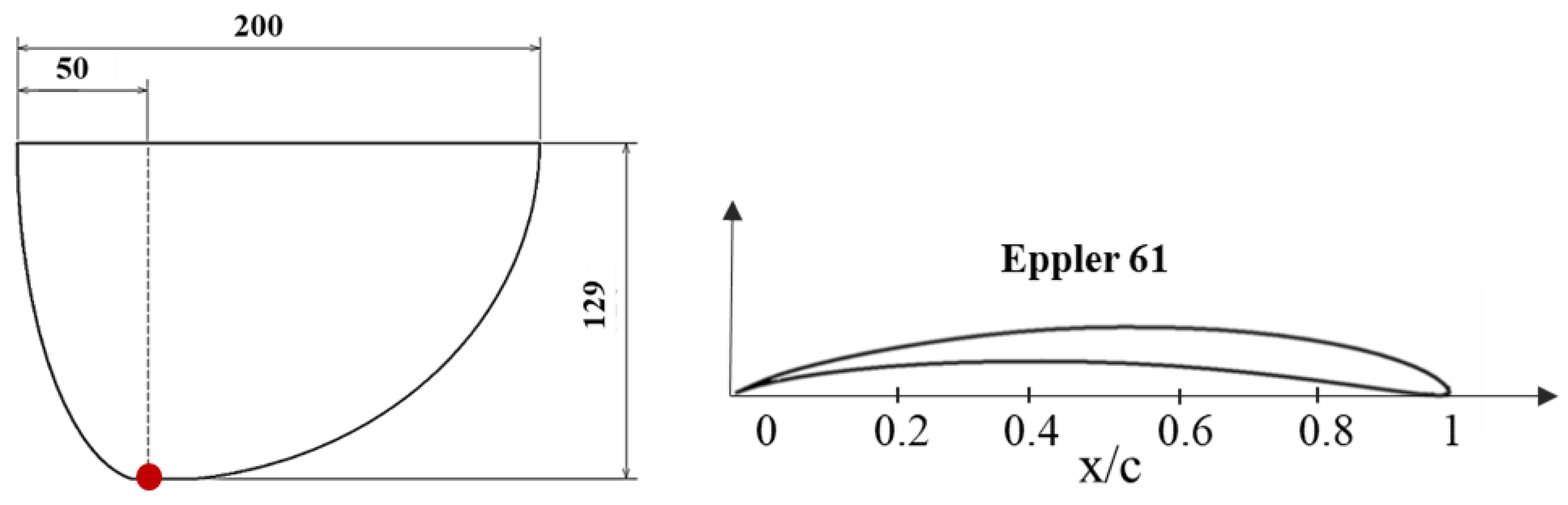
The geometry of this MAV consists of a Zimmerman wing platform with Eppler 61 airfoils. The Zimmerman wing is composed of two half ellipses joined at the reference point (red point) of Figure 2. For one half ellipse, this reference point corresponds to ¼ of the wing root chord and for the second one to ¾. The fuselage is designed with Whitcomb airfoils. These features were selected according to the main aerodynamic parameters: maximum lift to drag ratio, , maximum lift coefficient, , and minimum drag coefficient, . Figure 2 shows the configuration of the wing where x/c is the non-dimensional chord.
This MAV model was designed with the purpose of modifying its wings during flight. In particular, the camber and thickness of the wing will be the only parameters which could change during flight while the chord and wingspan must remain constant. Therefore, the ultimate goal of this MAV is to improve the aerodynamic performances in terms of maximizing the autonomy and range depending on the flight phases in where it is immersed. To obtain the curvature and thickness variations, the authors in [10] tested experimentally the wings with smart materials.
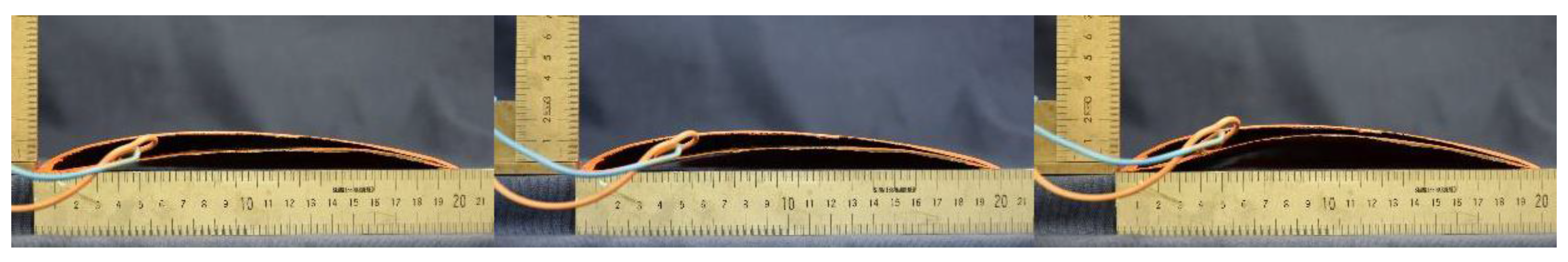
Especially, they selected Micro-Fiber Composite (MFC) piezoelectric actuators since these present the ability of using them in elongation and contraction depending on the applied voltage and are low-cost devices with a low voltage operation. Moreover, these devices present other advantages such as durability, flexibility, directional actuation, increased damage tolerance and higher efficiency than other design strategies as mechanical devices. These actuators were installed on the lower surface of the wings and the voltage range was between 0 V and 5 V (see Figure 3). Figure 3 shows the Eppler 61 airfoils in different stages. Therefore, the airfoil on the left side corresponds to the Eppler 61, that is, with no voltage. However, the airfoil at the center presents a voltage of 2.8 V and on the right side, the airfoil corresponds to the maximum voltage, 5 V.
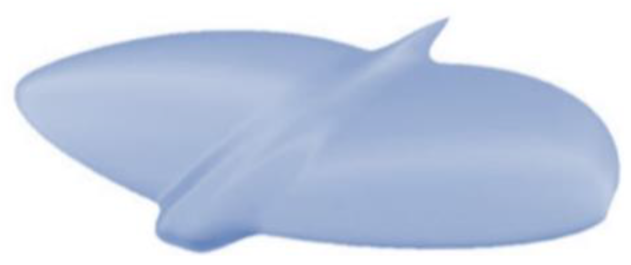
The MAV was designed in three different configurations according to the previous wing airfoils by the CATIA software. All configurations were manufactured by using a 3D printing machine (low-cost) and the additive material used was Polylactic Acid (PLA). The additive material was deposited layer by layer having a horizontal surface as a reference. Due to the complex geometry of this MAV model, it had to be printed in two halves independently. The first layer started on the fuselage airfoil and continued in a vertical direction to the tip of the wing. After manufacturing, a sanding task on the surface of the wings was required to eliminate possible burrs deposited over them. These MAV models were tested in the wind tunnel. The geometry of this MAV can be seen in Figure 4.
4. Computational Fluid Mechanics Investigation
4.1. Ansys-Fluent 2020
A numerical study based on Computational Fluid Dynamics (CFD) was carried out in order to compare the data to the wind tunnel measurements. CFD is a numerical technique implemented in computers focused on simulating the aerodynamic flow by discretizing the control volume into smaller control volumes where the fluid mechanics’ equations are solved in each of them. For this purpose, the commercial software Ansys-Fluent 2020 was used.
Firstly, the geometry is imported from a simplified 3D model of the morphing MAV (see Section 3). The simplified model is designed without the fuselage to improve the performance of simulations in terms of capacity and time. As the main objective of this paper is to analyze the deformation of the wing structure in terms of curvature and thickness, and compare them with experimental data, three models were required. Therefore, the first simplified model was the MAV with no wing deformation corresponding to 0 V (Eppler 61 airfoils without deformation), the second one presented a semi-deformation corresponding to 2.8 V and the last one was the MAV with the maximum deformation in curvature and thickness corresponding to 5 V (maximum voltage applied).
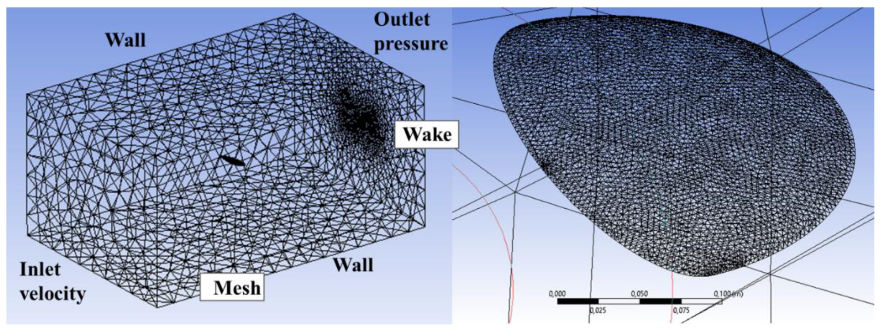
Secondly, the control volume is defined according to the dimensions of the simplified model. The boundary conditions of the control volume are delimited depending on the position of the model inside of it (it can be observed in Figure 5). Therefore, the face in front of the leading edge of the wing corresponds to the inlet and the one behind the trailing edge of the wing is the outlet. The rest of the boundaries are walls. The boundary conditions are defined as the velocity inlet and pressure outlet (see Figure 6). In this fluid control volume, as one of the goals is to study the airflow wake, it was more convenient to divide the region into two to obtain a higher resolution in the interest region; consequently, one volume encompassing only the wake (wake volume, see Figure 5) to generate a smoother mesh, therefore, the flow equations will be solved in a higher number of cells and the final resolution of simulations could be better. The second volume (control volume, see Figure 5) contains a mesh with larger cell dimensions to reduce calculation time. Figure 6 shows the control volume and wake volume meshed and Table 2 shows the features of the mesh used for this analysis.
Once the mesh is generated, the simulation starts by using the appropriate solver. In this paper, as the free stream velocity of experimental tests is 10 m/s and the airflow is an incompressible, subsonic and steady fluid flow, the solver required was the pressure-based approach. This solver obtains the velocity field under these conditions by applying the mechanics fluid equations. The turbulence model used for this numerical study was the k-ε model. This model is based on solving two variables: k, which is the turbulent kinetic energy and ε which is the dissipation rate of k. This turbulence model simulates the viscous sublayer flow reaching the buffer region. The smooth curvature of the wing makes this turbulence model ideal for this purpose. The boundary conditions were defined as 10 m/s for the inlet and ∆P = 0 (gauge pressure) for the outlet since the outlet pressure is defined as atmospheric pressure, due to this the section is located far away from the trailing edge of the MAV. All numerical simulations are initialized from the inlet condition and the fluid mechanics equations are calculated for a maximum of 1000 iterations.
4.2. Computational Fluid Mechanics Results
4.2.1. Measurement Planes
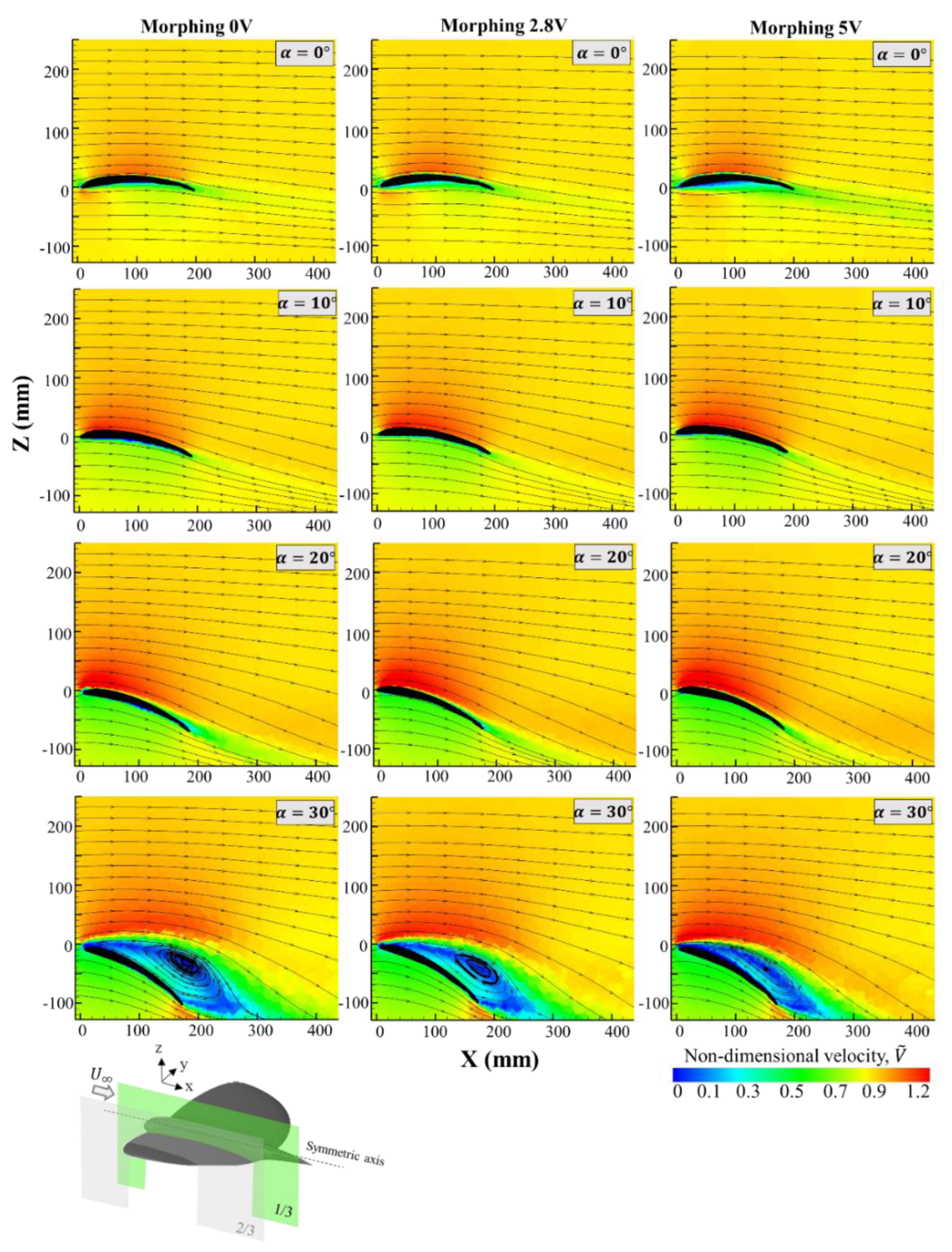
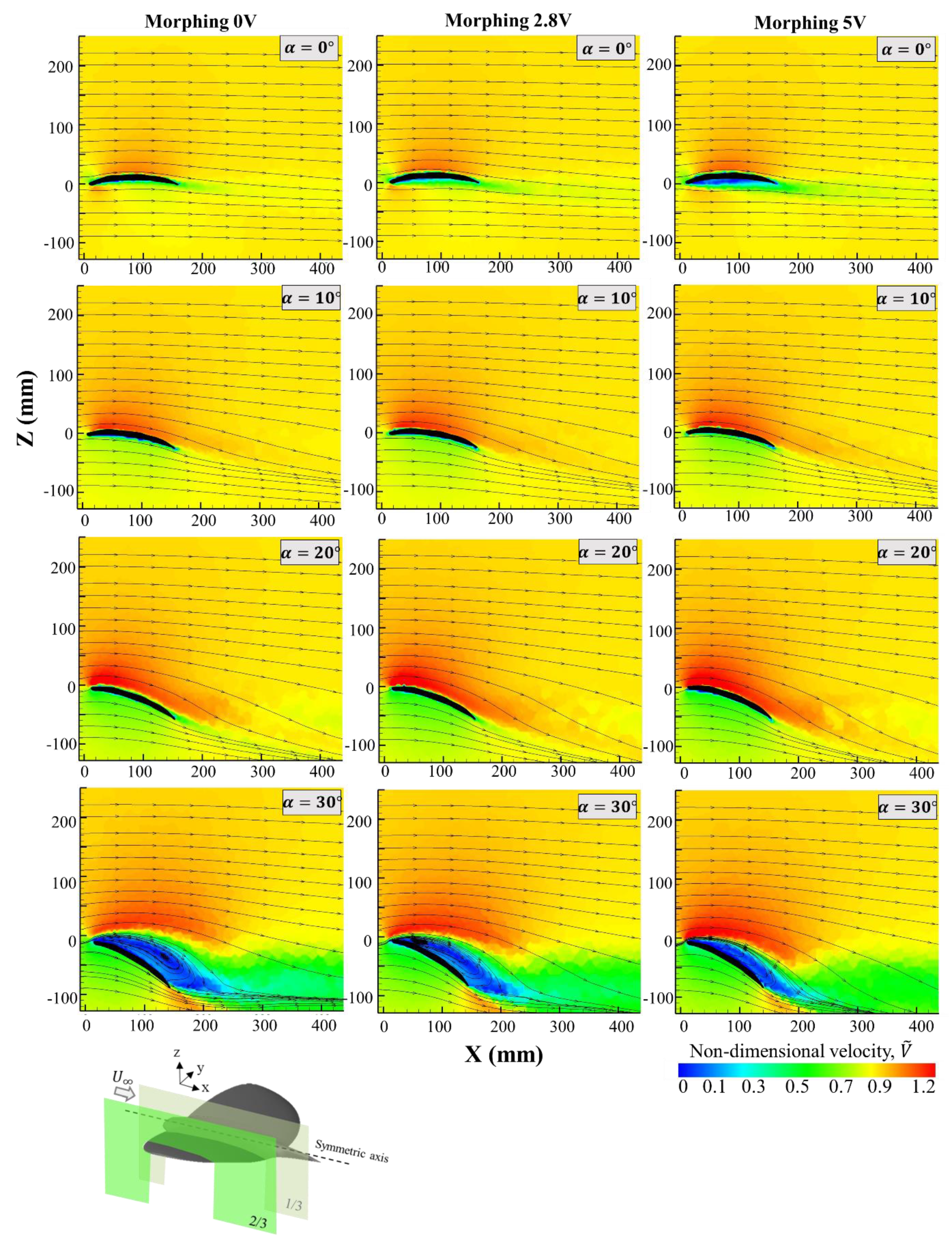
Figure 7, Figure 8 and Figure 9 show a flow visualization of the three wing configurations morphing 0 V (without wing deformation), morphing 2.8 V (semi wing deformation) and morphing 5 V (maximum wing deformation) from different positions and for several angles of attack. These results are defined as the non-dimensional velocity in respect to the free stream velocity of the wind tunnel (). The first two Figure 7 and Figure 8 correspond to the perpendicular planes located at 1/3 and 2/3 of the semi-wingspan () with respect to the symmetric axis of the MAV, respectively. In this case, the non-dimensional velocity is where and are the velocity components in the X-axis and Z-axis, respectively. However, the results presented in Figure 9 correspond to the non-dimensional transversal velocity , where is the velocity in Y-axis. The selected plane was located at three chords (3c) from the trailing edge of the MAV since it is far away from the model and the flow was able to obtain the damping condition. Both results were obtained with the purpose of analyzing the flow pattern from the cruise flight phase (α = 0°) to the stall condition where the flow is totally detached (α = 30°). Only the most relevant angles of attack are presented.
Similar aerodynamic behavior was observed in all wing configurations. The free stream velocity of 10 m/s, where streamlines are parallel to the X-axis, is presented by the orange region. Above the wing surface, the flow was accelerated by up to 20% more than the free stream velocity. Moreover, the velocities of this region along with the dimension of this area increased with the angle of attack. The region at the bottom of the wing (green region) represents velocities lower than the free stream velocity up to 30%. Behind the trailing edge of the wing, the thin region represents the wake where the velocities are between 10% and 20% lower than the free stream velocity. At low angles of attack (α < 25°), the flow was still attached, showing these flow structures for the three wing configurations. However, at higher angles of attack (α 25°), the flow started detaching from the wing until the stall condition was reached 30°). In this angle of attack, the most significant structure is the recirculation bubble (blue region) that begins appearing from the angle of attack of 25°. Inside the recirculation bubble, the flow reached velocities near zero and streamlines show how the flow contained in that small region was recirculating. At that point, the airflow was completely detached from the surface of the wing. Consequently, the stall condition is presented for all wing configurations. A great difference between these three wing configurations is the size of the recirculation bubble. For the morphing 2.8 V (semi-deformation), the size of this flow structure is around 25% smaller than morphing 0 V (with no wing deformation). However, for the maximum wing deformation, this decrease is even higher, being around 50% smaller. As the starting point, this increase in curvature and thickness resulted in an improvement of the aerodynamic performance of the MAV since the flow is attached for a greater region.
In the planes located at 2/3 (Figure 8), as these are the nearest to the wing tip, the recirculation bubble presents a smaller dimension compared to those which were measured nearest the symmetric axis of the model (Figure 7). The fact of increasing curvature and thickness did not have any substantial effect at low angles of attack; however, it made a direct impact in the flow structure for high angles of attack (α > 25°).
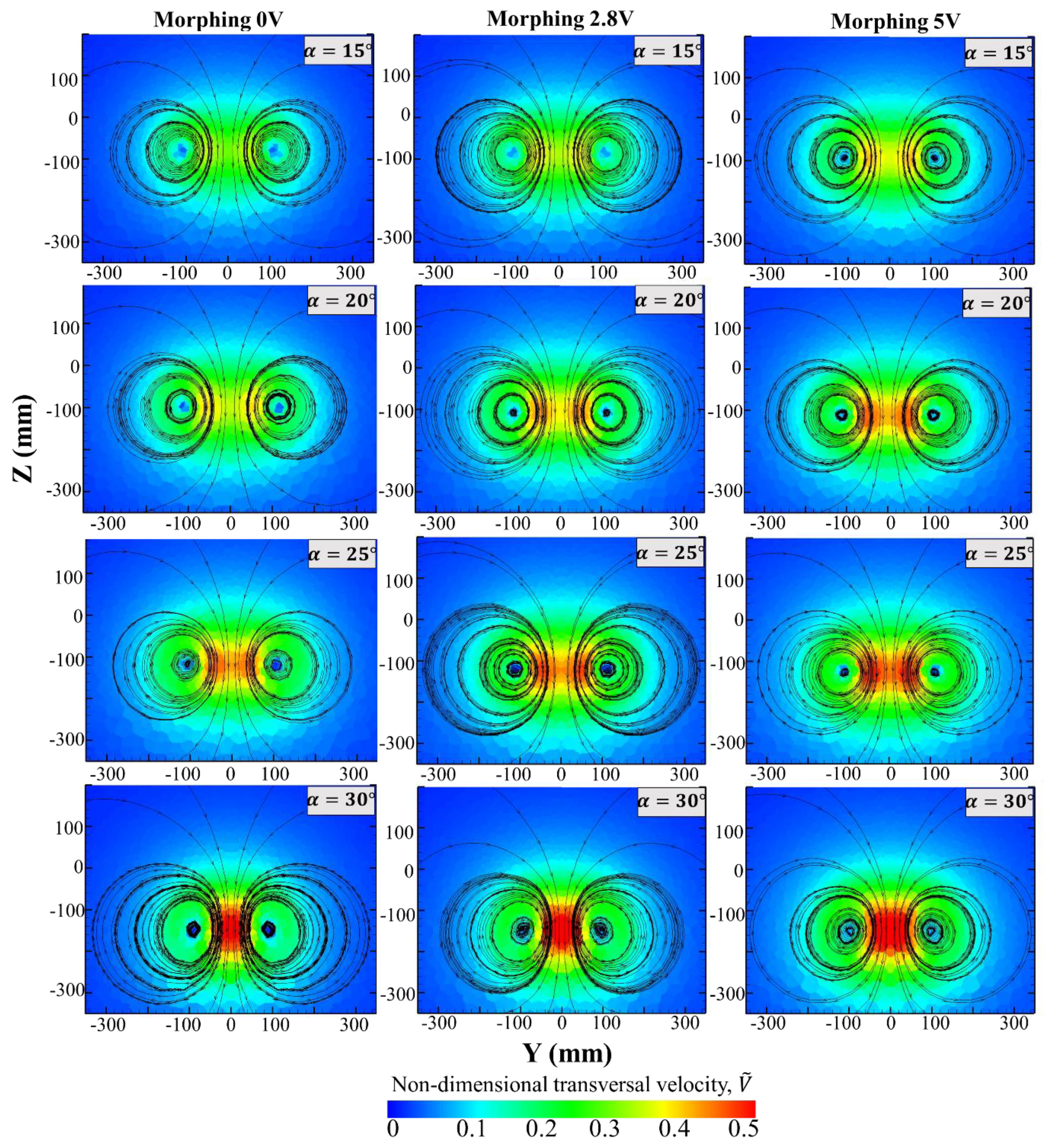
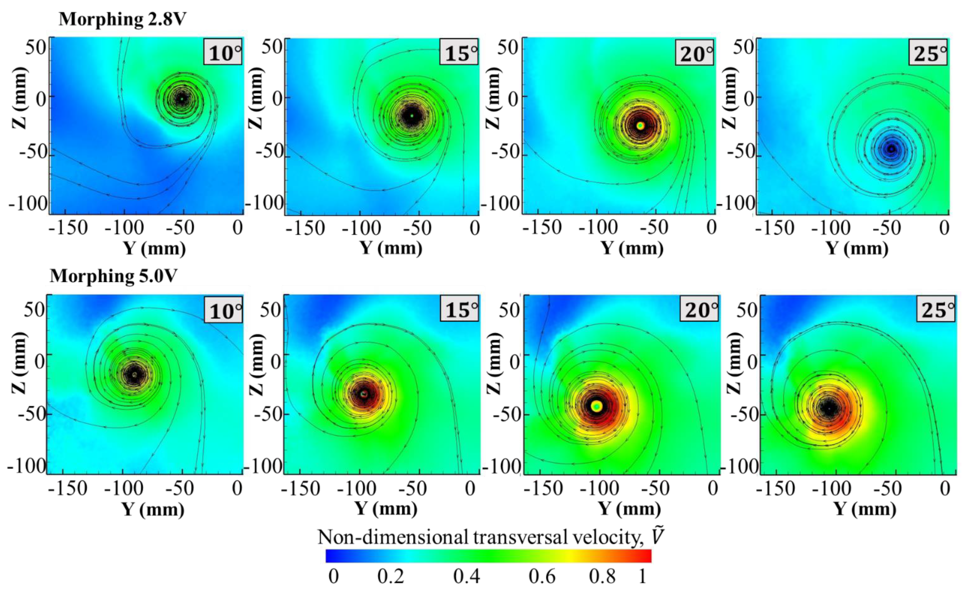
Regarding the transversal velocities (Figure 9), these results show the flow pattern of the wing tip vortices when they were projected from a perpendicular section to the air wake. The blue area corresponds to the area without any flow perturbations (free stream velocity) while inside of this, it can be seen the structure of the wake with two wing tip vortices due to the wing tips and joint between them due to the fuselage (red region).
In all of them, the center of all wing tip vortices, where the non-dimensional transversal velocity is zero, is represented by the circular streamlines and small blue region. Outside of that area, the transversal velocities are higher by 30% (green area) until reaching the highest values around 50% (red region) near the symmetric axis of the MAV (joint of two wing tip vortices). For low angles of attack (α 20°), the flow pattern of the two wing tip vortices is clearly defined, while for higher angles of attack (α > 20°) the joint region between them begins to predominate. As curvature and thickness start increasing, the region of wing tip vortices along with the joint region begin having a great dimension in both axis Y-axis and Z-axis. Moreover, the displacement of the wing tip vortices is presented. For all wing configurations, the centers of the vortices are placed at 0 mm in the Z-axis for the angle of attack of 0° (α = 0°) and they suffered a downward displacement of 13 mm (Z < 0 mm). At the same time, each vortex moves in the Y-axis direction to the symmetric axis, but in this case the displacement was smaller (around 5 mm).
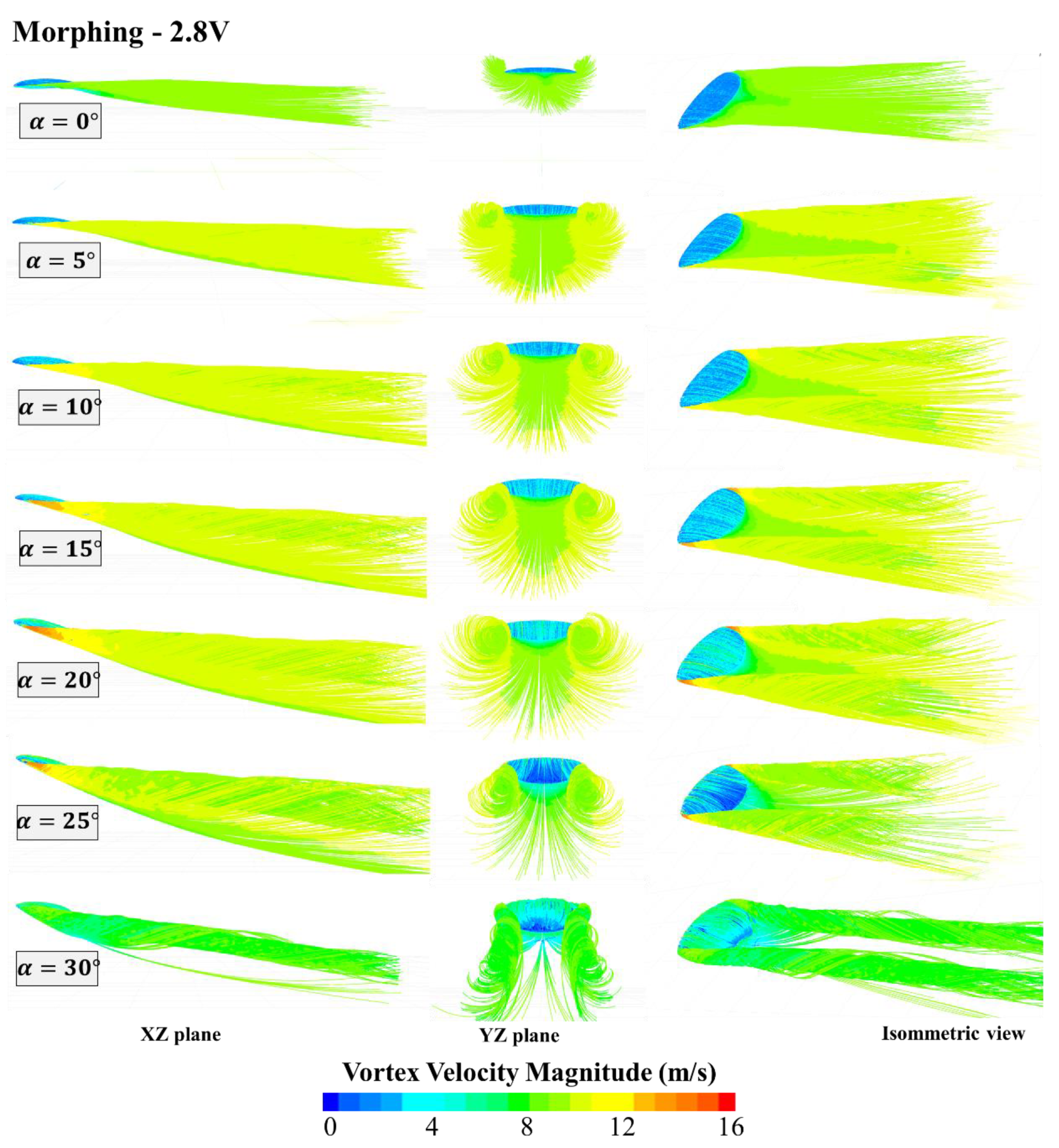
To complete the flow visualization, Figure 10 shows several perspectives of the wake structure for the MAV with semi-deformation in curvature and thickness (morphing 2.8 V). The air wake is presented in three views (XZ plane, YZ plane and isometric perspective). The vortex velocity magnitude (defined as ) presents the highest values near the wing tips and only for the angles of attack from 15° to 25°. It can be seen how the flow was attached until α = 25°. From that angle of attack on the vortex, the velocity magnitude of the wake begins decreasing and the streamlines over the wing surface start removing from it (see the blue surface in isometric view).
4.2.2. Lift and Total Aerodynamic Drag Coefficients and Lift/Drag Ratio
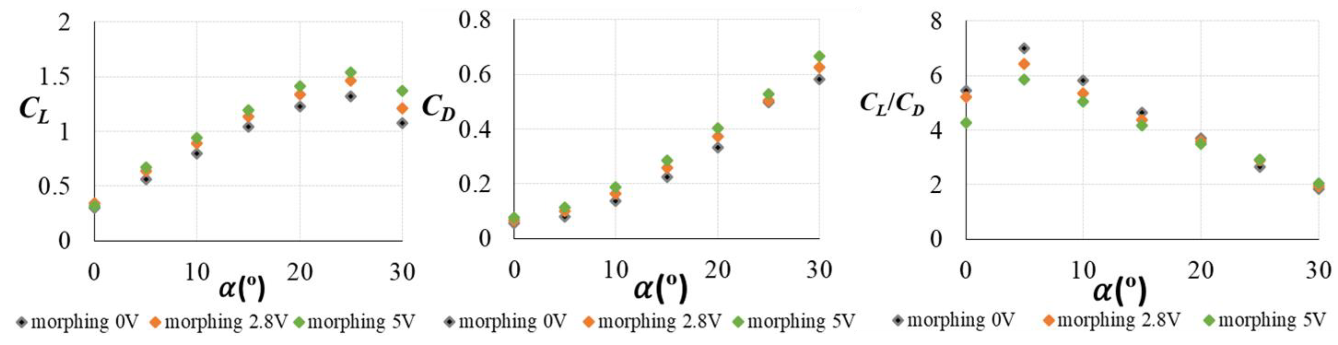
Figure 11 shows the lift coefficient, total aerodynamic drag coefficient and lift/drag ratio for all wing configurations. It can be seen that when the MAV wing increase curvature and thickness, the lift coefficient () increases for all angles of attack. However, the total aerodynamic drag () presents higher values as the wing increases its deformation. Consequently, the aerodynamic efficiency assessed by the lift/drag ratio, presents the lowest values for the fully deformed configuration (5 V) under angles of attack of 20° and lower.
5. Experimental Study
5.1. Wind Tunnel and Particle Image Velocimetry
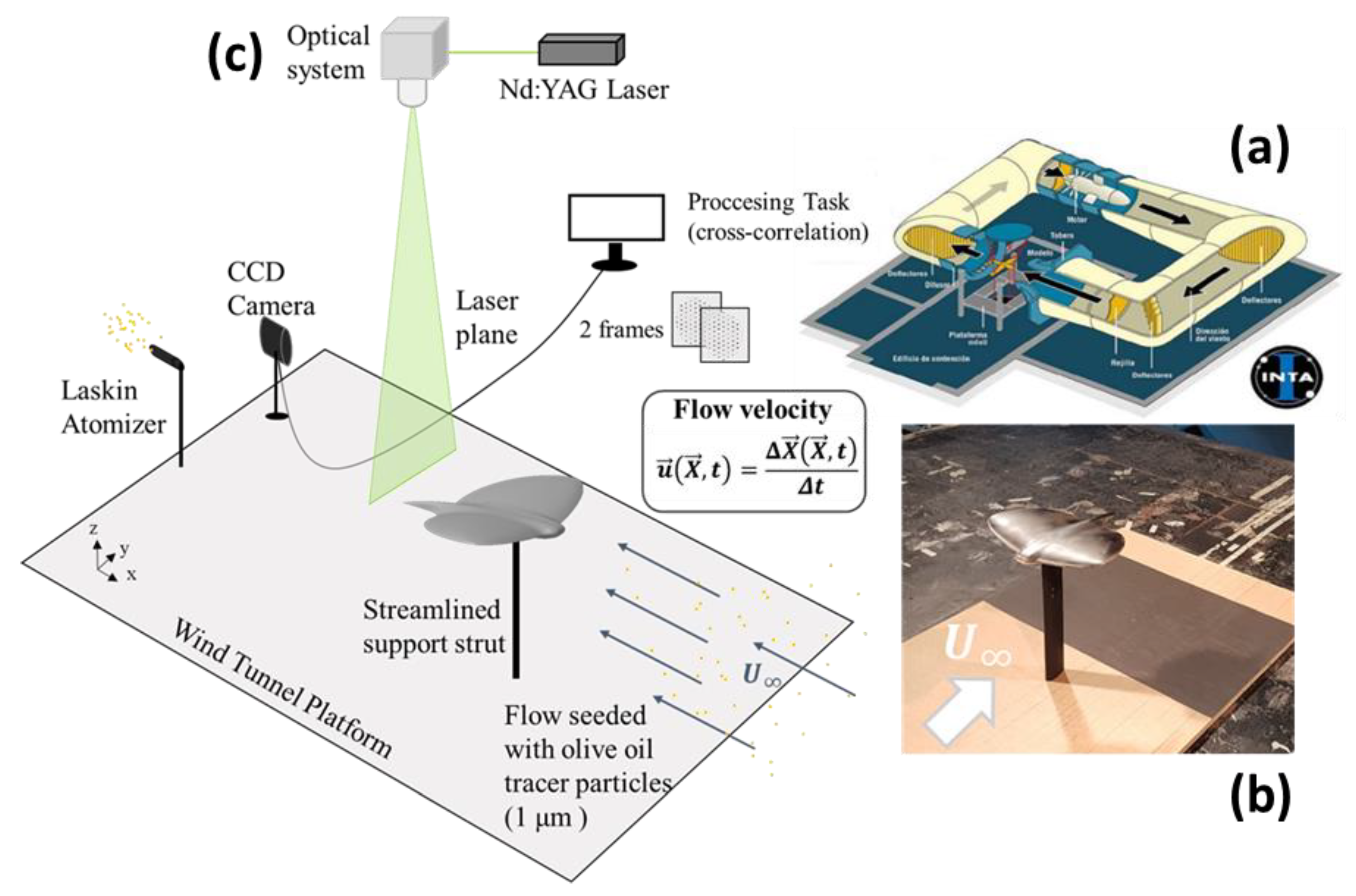
All experimental tests requiring Particle Image Velocimetry (PIV) were carried out in the Low-Speed Wind Tunnel 1 of the Instituto Nacional de Técnica Aeroespacial (INTA), located in Madrid (Spain). The configuration of this wind tunnel presents a close-circuit with an elliptical open test section (2 × 3 m2). The maximum airflow velocity in this wind tunnel is 60 m/s and the level of turbulence intensity is lower than 0.5%. The engine, which is placed at the opposite side of the test section, works at 420 V. In addition, there is a moving platform, where the scale models are placed, that was designed with streamlined edges (leading and trailing) in order to reduce the flow perturbations during experimental tests.
Particle Image Velocimetry is an advanced and non-intrusive experimental technique used to measure the airflow velocity. This technique is focused on obtaining pairs of flow images. Therefore, tracer particles must be seeded in the airflow reaching the flow velocity. Olive oil was used for this purpose and the diameter of these tracer particles was around 1 μm. This particle size was obtained by a compressor connected to Laskin atomizers (the pressure was 4 bars). A laser plane goes through the airflow and the tracer particles are illuminated. A neodymium-doped yttrium aluminum garnet (Nd: YAG) laser is generated by a combination of spherical and cylindrical lenses and it is pulsed twice with a time interval of 22 μs. A CCD (Charged-Coupled Device) camera with 2048 × 2048 pixels captures the flow images at the same time the laser is pulsed. This action is performed by a synchronizer and the processing task for obtaining the flow velocity is developed by a software (Insight). The average displacement of tracer particles between the two flow images is calculated by FFT (Fast Fourier Transform) in all 32 × 32 pixels interrogation windows. A final post-processing task is required in order to eliminate spurious velocity vectors. In Table 3, the parameters of Particle Image Velocimetry used for developing all experimental tests are shown.
The selected sections to develop the experimental tests were perpendicular and transversal planes to the scale models according to the chord distance and angle of attack in order to visualize the flow from several angles. From this information, all aerodynamics coefficients could be obtained with the purpose to compare them with numerical data. To obtain each of these planes, an average plane of the velocity field of 200 pairs of images was required. Moreover, all scaled models were painted in black to avoid possible reflections of laser pulses. The models were placed in the moving platform with a streamlined support strut to minimize flow perturbations. Each of the morphing configurations was manufactured by additive manufacturing with ABS as the selected material to maintain the required stiffness to perform the experimental tests. The camera CCD was placed far away from the models to capture the flow images without perturbing the airflow.
The experimental study consisted in obtaining several transversal planes situated downstream of the trailing edge of the model and from the angles of attack of 0° to 30° with a step of 5°. The freestream velocity of the wind tunnel was 10 m/s; therefore, the Reynolds number based on the root chord (c = 200 mm) was 1.3 × 10⁵. Moreover, perpendicular planes to the wing were obtained for the same angles of attack and with the same freestream velocity. In Figure 12, the experimental set-up is shown.
5.2. PIV Results
Figure 13 shows the non-dimensional transversal velocity obtained by measuring in the wake using Particle Image Velocimetry. The most relevant angles of attack are presented and only for the wing configuration of 2.8 V and 5 V. From these data, the aerodynamic performances were calculated.
5.3. Balance Measurements
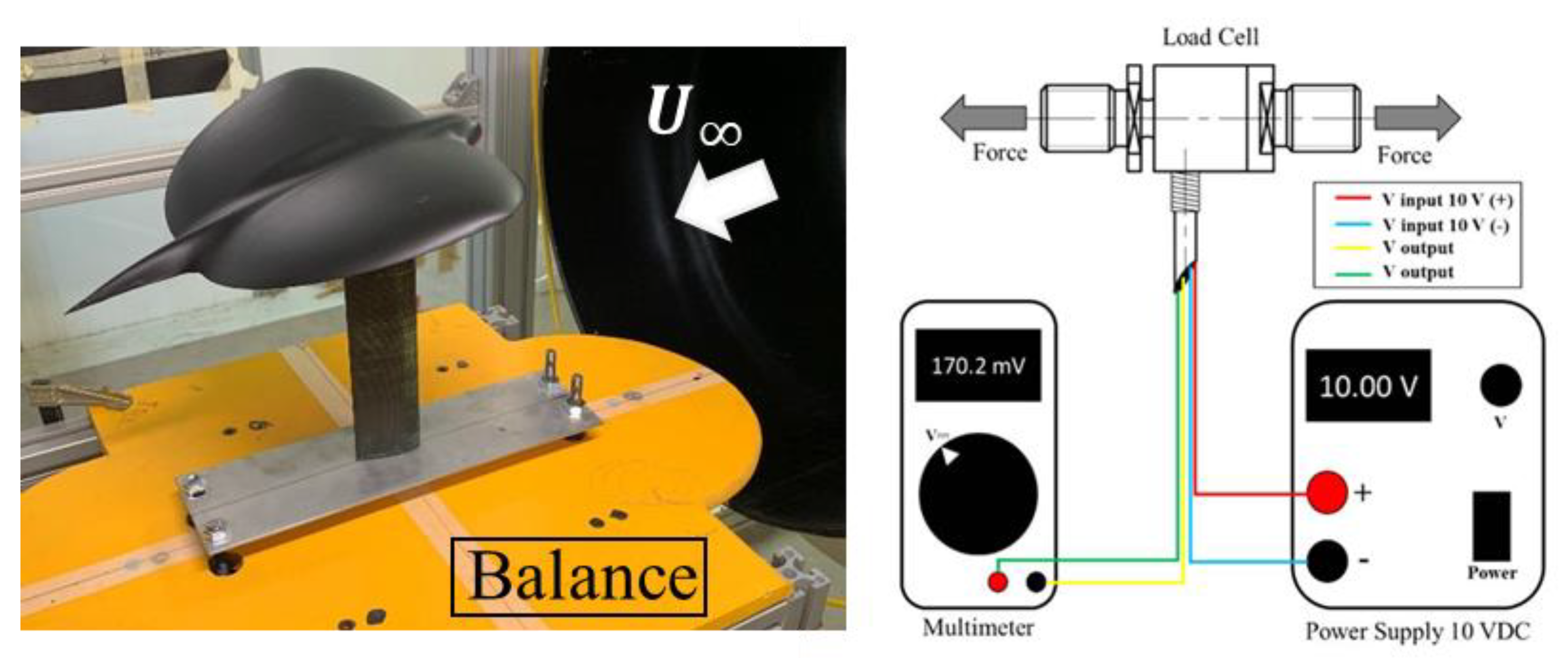
The balance was designed according to the dimensions of the test section of the Westenberg Wind Tunnel. Moreover, the front part of this balance was designed with a streamlined structure of aluminum sheet to avoid possible airflow interferences. The balance needs to be connected to an electrical supply. In this case, the load cell requires a DC voltage source regulated between 1 and 10 V (see Figure 16). For this purpose, an adjustable power supply (Transfer Multisort Elektronik (TEM) MANSON EP-613) was used. The aerodynamic force was measured by the load cell indirectly. Therefore, this value is given in voltage and it was provided by a multimeter (Fluke MetraHIT 16) (see Figure 14).
To perform the experimental tests, a previous calibration of all instruments was needed to reduce systematic errors. This process was performed using an inclinometer, an alignment laser, a small crane with a pulley hanging different calibrated weights, a DC power source, a nylon thread, a multimeter and a hook to hang the selected weights.
The three wing configurations were tested to obtain the total aerodynamic drag coefficient for all angles of attack (from α = 0° to 30°).
6. Comparative Analysis: CFD vs. Experimental
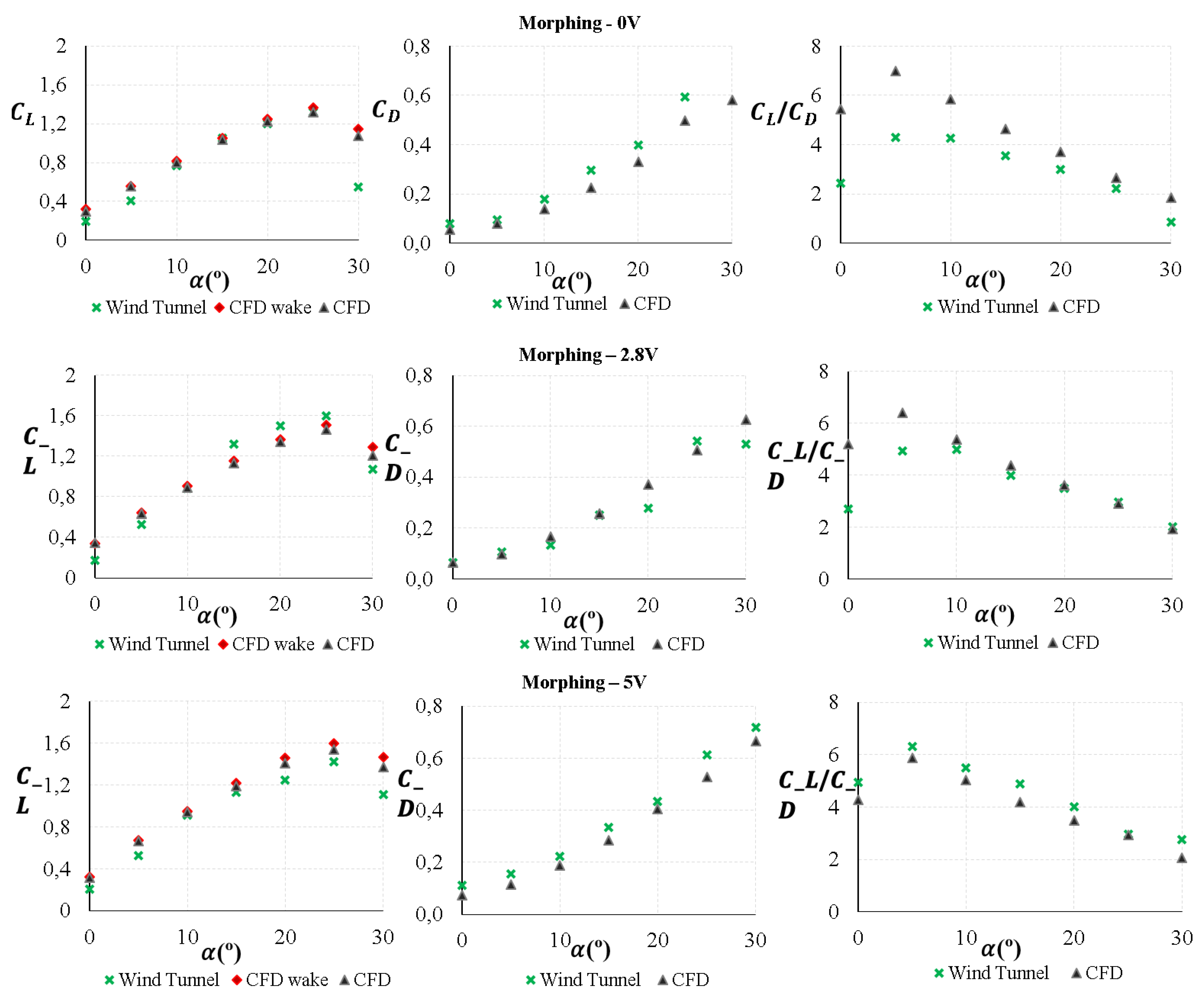
Figure 15 shows the lift coefficient (left), total aerodynamic drag coefficient (center) and lift/drag ratio (right) according to the angle of attack for the three configurations (with no wing deformation, 0 V, semi-deformation, 2.8 V and maximum deformation, 5 V) for case U∞ = 10 m/s and β = 0°. In the results related to lift coefficient, the experimental data were obtained by Particle Image Velocimetry in the wind tunnel. However, the total aerodynamic drag coefficient was measured by the balance. The CFD wake data were defined as the wake survey analysis where the lift coefficient can be obtained by using the Maskell theory (Section 2). Finally, the direct numerical data obtained from the numerical simulation with Ansys Fluent are presented by CFD.
The lift coefficient of all wing configurations shows the typical linear segment that increased from 0° to the critical angle of attack where the maximum value was obtained (maximum lift coefficient). At that point, the flow starts detaching from the surface of the wing until reaching the total stall condition where the flow is completely detached.
For the wing without deformation (morphing 0 V), the maximum lift coefficient was 1.4 for the angle of attack of 25°. However, for the wing with deformation (2.8 and 5 V) that value was higher, reaching values around 1.6. Therefore, there is a direct correlation between the wing curvature and lift coefficient. It can be noticed that the data obtained by the different methods gave very similar results. The error between numerical and experimental data was between 5 and 8%.
In Figure 16, the numerical data from the Ansys Fluent simulations and experimental data from wind tunnel tests are presented for all morphing wing configurations. On the left side, the lift coefficient is presented and on the right side the total aerodynamic drag coefficient.
Comparing the three wing configurations, it can be obtained that the wing without modification (0 V) presented the lowest lift coefficients for all angles of attack. The other two wing configurations (semi-deformation (2.8 V) and maximum deformation (5 V)) presented a similar aerodynamic behavior, although the configuration with maximum curvature (5 V) showed slightly higher values than the semi-deformation (2.8 V). From this data, as the first starting point, it could be feasible to assume that the wing with maximum curvature and thickness (5 V) would be the best configuration in terms of lift. However, the final objective is to improve the aerodynamic performance of this MAV; therefore, the aerodynamic drag must be taken into account. In terms of aerodynamic drag, the induced drag and total aerodynamic drag coefficients were obtained to reach the optimal aerodynamic performance.
With regards to the total aerodynamic drag coefficient, the configuration that presented the highest values of it was the one with the maximum curvature and thickness of the wing that corresponds to the maximum deformation (5 V) of the airfoil generated the lowest aerodynamic efficiency (CL/CD).
It is interesting to see how increasing the curvature and thickness of the wing had a double impact on the overall aerodynamic performance. Although this configuration presented the benefit of a higher lift during all flight phases, the aerodynamic drag resulted to be the highest, giving a negative effect on the aerodynamics of this vehicle.
Consequently, the aerodynamic drag must be reduced to be able to implement this aerodynamic vehicle in the future. The fact of having the highest lift in all angles of attack as well as the lowest total aerodynamic drag gives the optimal aerodynamic performance of an aircraft. Taking into account all this, a compromise solution between lift and total aerodynamic drag is required to have a worthy implementation. Therefore, the morphing 2.8 V model would be the best option regarding aerodynamic performance since the maximum lift coefficient was around 1.5 (similar to the maximum deformation and higher than morphing 0 V) and the total aerodynamic drag coefficient was the lowest for all angles of attack.
7. Conclusions
In this paper, an experimental and numerical CFD analysis of the wake structure of an MAV with an adaptive wing geometry was studied. Three wing configurations were tested: morphing 0 V (Eppler 61 airfoil), morphing 2.8 V (semi-deformation of the wing) and morphing 5 V (maximum deformation in curvature and thickness). Several flight phases were analyzed: from cruise condition (α = 0°) to stall condition (α = 30°).
The comparative analysis on morphing UAV with different wing configurations was studied based on curvature and thickness deformations with several angles of attack by wind tunnel testing and numerical simulations. The experimental data were obtained using Particle Image Velocimetry and balance while the numerical analysis was performed using the software Ansys Fluent 2020. Non-dimensional velocity maps allowed the analysis of the flow in the wake of the model and the detachment generated at higher angles of attack than 25°. The wing deformation was positive for the aerodynamic performance of the MAV since the flow was attached for a greater region. The vortex generated by the wing tips and their interaction between them was also studied in a transverse plane. Finally, the numerical and experimental results of lift and drag coefficients were also compared, showing small differences between them of 5 and 8%. From the analysis of the results with the variations of the wing geometry, it was concluded that the MAV configuration with semi-deformation (morphing 2.8 V) presented an improvement in the aerodynamic performance than the other two wing configurations tested, with a higher lift and lower total aerodynamic drag coefficient for all angles of attack.
Author Contributions
Conceptualization, R.B. and Á.R.-S.; methodology, R.B. and Á.R.-S.; software, E.B. validation, R.B., Á.R.-S. and E.B.; formal analysis, R.B., Á.R.-S. and E.B.; investigation, R.B., Á.R.-S. and E.B.; resources, E.B.; data curation, R.B., Á.R.-S. and E.B.; writing—original draft preparation, R.B., Á.R.-S. and E.B.; writing—review and editing, R.B., Á.R.-S. and E.B.; visualization, R.B. and Á.R.-S.; supervision, R.B. and Á.R.-S.; project administration, R.B. and Á.R.-S.; funding acquisition, R.B. and Á.R.-S. All authors have read and agreed to the published version of the manuscript.
Funding
The investigation was funded by the Spanish Ministry of Defense under the program 464A 64 1999 14205005 “Termofluidodinámica” with internal code IGB 99001 of ‘’Instituto Nacional de Técnica Aeroespacial Esteban Terradas’’ (INTA).
Acknowledgments
We thank all engineers and analysts of the Aerodynamics Department of ‘’Instituto Nacional de Técnica Aeroespacial Esteban Terradas’’ (INTA).
Conflicts of Interest
The authors declare no conflict of interest. The funders had no role in the design of the study; in the collection, analyses, or interpretation of data; in the writing of the manuscript, or in the decision topublish the results.
References
- Moschetta, J.L. The aerodynamics of micro air vehicle: Technical challenges and scientific issues. Int. J. Eng. Syst. Model. Simul. 2014, 6, 134–148. [Google Scholar] [CrossRef]
- Hassanalian, M.; Abdelkefi, A. Design and manufacture of a fixed wing MAV with Zimmerman planform. In Proceedings of the AIAA SciTech, 54th AIAA Aerospace Sciences Meeting, Kissimmee, FL, USA, 4–8 January 2016. AIAA 2016-1743. [Google Scholar] [CrossRef]
- Marek, P.L. Design, Optimization and Flight Testing of a Micro Air Vehicle. Ph.D. Thesis, University of Glasgow, Glasgow, UK, 2008. [Google Scholar]
- Flake, J.; Frischknecht, B.; Hansen, S.; Knoebel, N.; Ostler, J.; Tuley, B. Development of the Stableyes Unmanned Air Vehicle. In Proceedings of the 8th International Micro Air Vehicle Competition, Tucson, AZ, USA, 10 April 2004; pp. 1–10. [Google Scholar]
- Stanford, B.; Sytsma, M.; Albertani, R.; Viieru, D.; Shyy, W.; Ifju, P. Static aeroelastic model validation of membrane micro air vehicle wings. AIAA J. 2007, 45, 2828–2837. [Google Scholar] [CrossRef]
- Min, Z.; Kien, V.K.; Richard, L.J.Y. Aircraft morphing wing concepts with radical geometry change. IES J. Part A Civ. Struct. Eng. 2010, 188–195. [Google Scholar] [CrossRef]
- Barbarino, S.; Bilgen, O.; Ajaj, R.M.; Friswell, M.I.; Inman, D.J. A review of morphing aircraft. J. Intell. Mater. Syst. Struct. 2011, 22, 823–877. [Google Scholar] [CrossRef]
- Sun, J.; Guan, Q. Morphing aircraft based on smart materials and structures: A state-of-the-art review. Intell. Mater. Syst. Struct. 2016, 27, 2289–2312. [Google Scholar] [CrossRef]
- Barcala-Montejano, M.A.; Rodríguez-Sevillano, A.; Crespo-Moreno, J.; Bardera Mora, R.; Silva-González, A.J. Optimized performance of a morphing micro air vehicle. In Proceedings of the Unmanned Aircraft Systems (ICUAS), 2015 International Conference, Denver, CO, USA, 12 June 2015. [Google Scholar] [CrossRef]
- Barcala-Montejano, M.A.; Rodríguez-Sevillano, A.; Bardera-Mora, R.; García-Ramirez, J.; Leon-Calero, M.; Nova-Trigueros, J. Development of a morphing wing in a micro air vehicle. In Proceedings of the 8th ECCOMAS Thematic Conference pon Smart Structures and Materials, SMART 2017, Madrid, Spain, 5–8 June 2017. [Google Scholar]
- Drela, M. Flight Vehicle Aerodynamics; The MIT Press: Cambridge, MA, USA, 2014; Chapter 5. [Google Scholar]
- Fan, Y.; Li, W. Review of far-field drag decomposition methods for aircraft design. J. Aircr. 2019, 56. [Google Scholar] [CrossRef]
- Betz, A. A method for the direct determination of profile drag. Z. Für Flugtech. Und Mot. 1925, 16, 42–44. [Google Scholar]
- Maskell, E.C. Progress towards a Method for the Measurement of the Components of the Drag of a Wing of Finite Span; RAE Technical Report 72232; Royal Aircraft Establishment RAE: Farnborough, Hampshire, 1972. [Google Scholar]
- Brune, G.W. Quantitative Three-Dimensional Low-Speed Wake Surveys; Boeing Commercial Airplane Group Seattle: Washington, DC, USA, 1991. [Google Scholar]
- Kusunose, K. Development of a universal wake survey data analysis code. In Proceedings of the 15th Applied Aerodynamics Conference, Atlanta, GA, USA, 23–25 June 1997. AIAA Paper 1997-2294. [Google Scholar] [CrossRef]
- Cummings, R.M.; Giles, M.B.; Shrinivas, G.N. Analysis of the elements of drag in three-dimensional viscous and inviscid flows. In Proceedings of the 14th Applied Aerodynamics Conference, New Orleans, LA, USA, 17–20 June 1996. AIAA Paper 1996-2482-CP. [Google Scholar] [CrossRef] [Green Version]
- Sor, S.; Bardera, R.; García-Magariño, A.; Matías García, J.; Donoso, E. Development and characterization of a low-cost wind tunnel balance for aerodynamic drag measurements. Eur. J. Phys. 2019, 40, 045002. [Google Scholar] [CrossRef]
Figure 1.
Control volume defined for the numerical and experimental analysis.

Figure 2.
Zimmerman wing plantform (left) and Eppler 61 wing airfoil (right). Dimensions in mm.

Figure 3.
Eppler 61 airfoil with 0 V (left), applied voltage of 2.8 V (center) and 5 V (right). Ref. [10].
Figure 3.
Eppler 61 airfoil with 0 V (left), applied voltage of 2.8 V (center) and 5 V (right). Ref. [10].

Figure 4.
MAV with morphing geometry.

Figure 5.
Definition of boundary conditions for numerical simulations. (, .

Figure 6.
Control volume and wake volume meshed (left) and unstructured mesh of the MAV (right). (, ).
Figure 6.
Control volume and wake volume meshed (left) and unstructured mesh of the MAV (right). (, ).

Figure 7.
Non-dimensional velocity maps at 1/3 for all wing configurations: morphing 0 V, 2.8 V and 5 V (, ).
Figure 7.
Non-dimensional velocity maps at 1/3 for all wing configurations: morphing 0 V, 2.8 V and 5 V (, ).

Figure 8.
Non-dimensional velocity maps at 2/3 for all wing configurations: morphing 0 V, 2.8 V and 5 V (, ).
Figure 8.
Non-dimensional velocity maps at 2/3 for all wing configurations: morphing 0 V, 2.8 V and 5 V (, ).

Figure 9.
Non-dimensional transversal velocity maps for all wing configurations: morphing 0 V, 2.8 V and 5 V (, ).
Figure 9.
Non-dimensional transversal velocity maps for all wing configurations: morphing 0 V, 2.8 V and 5 V (, ).

Figure 10.
Vortex velocity magnitude for the morphing 2.8 V MAV (semi deformation of the wing) (, ).
Figure 10.
Vortex velocity magnitude for the morphing 2.8 V MAV (semi deformation of the wing) (, ).

Figure 11.
Lift coefficient (left), total aerodynamic drag coefficient (center) and lift/drag ratio (, ).
Figure 11.
Lift coefficient (left), total aerodynamic drag coefficient (center) and lift/drag ratio (, ).

Figure 12.
Low-Speed Wind Tunnel (a), scaled model inside the wind tunnel test section (b) and Particle Image Velocimetry set-up (c).
Figure 12.
Low-Speed Wind Tunnel (a), scaled model inside the wind tunnel test section (b) and Particle Image Velocimetry set-up (c).

Figure 13.
Non-dimensional transversal velocity maps for morphing 2.8 V and 5 V (wind tunnel data).

Figure 14.
MAV attached to the balance (left) and electrical connections of load cell to multimeter and power supply (right).
Figure 14.
MAV attached to the balance (left) and electrical connections of load cell to multimeter and power supply (right).

Figure 15.
Control volume and wake volume meshed (left) and unstructured mesh of the MAV (right). (, ).
Figure 15.
Control volume and wake volume meshed (left) and unstructured mesh of the MAV (right). (, ).

Figure 16.
Control volume and wake volume meshed (left) and unstructured mesh of the MAV (right). (, ).
Figure 16.
Control volume and wake volume meshed (left) and unstructured mesh of the MAV (right). (, ).


Table 1.
MAV features.
| Parameter | Value |
|---|---|
| Wing tip chord | 0.025 m |
| Wing root chord | 0.200 m |
| Taper ratio | 0.124 |
| Aspect ratio | 2.500 |
| Wingspan | 0.320 m |
| Mean aerodynamic chord | 0.141 m |
| Mean geometry chord | 0.127 m |
| Wing reference area | 0.040 m2 |
| Dihedral length | 10° |
| Fuselage length | 0.3 m |
| Fuselage width | 0.06 m |
Table 2.
Mesh features.
| Parameter | Value |
|---|---|
| Mesh type | Unstructured mesh |
| Smoothing | Medium |
| Inflation | Smooth |
| Relevant center | Fine |
| Span angle center | Fine |
| Maximum layers | 5 |
| Transition ratio | 0.3 |
| Minimum size | 5.7 mm |
| Maximum size | 116 mm |
| Growth rate | 1.2 |
| Nodes | 85,437 |
| Elements | 487,099 |
Table 3.
Particle Image Velocimetry features.
| Parameter | Value |
|---|---|
| At (time interval between laser pulses) | 22 μs |
| Camera CCD | Nikon NIKKOR 50 mm 1:1.4D |
| w (interrogation window size) | 32 × 32 pixels |
| Processing | 50% overlapping (Nyquist criteria). The correlation peak is adjusted to the subpixel accuracy Gaussian curve. |
| Post-processing algorithm | Local mean filter with a size of 3 × 3 pixels |
Publisher’s Note: MDPI stays neutral with regard to jurisdictional claims in published maps and institutional affiliations. |
© 2021 by the authors. Licensee MDPI, Basel, Switzerland. This article is an open access article distributed under the terms and conditions of the Creative Commons Attribution (CC BY) license (https://creativecommons.org/licenses/by/4.0/).
Share and Cite
MDPI and ACS Style
Bardera, R.; Rodríguez-Sevillano, Á.A.; Barroso, E. Numerical and Experimental Study of Aerodynamic Performances of a Morphing Micro Air Vehicle. Appl. Mech. 2021, 2, 442-459. https://0-doi-org.brum.beds.ac.uk/10.3390/applmech2030025
AMA Style
Bardera R, Rodríguez-Sevillano ÁA, Barroso E. Numerical and Experimental Study of Aerodynamic Performances of a Morphing Micro Air Vehicle. Applied Mechanics. 2021; 2(3):442-459. https://0-doi-org.brum.beds.ac.uk/10.3390/applmech2030025
Chicago/Turabian StyleBardera, Rafael, Ángel A. Rodríguez-Sevillano, and Estela Barroso. 2021. "Numerical and Experimental Study of Aerodynamic Performances of a Morphing Micro Air Vehicle" Applied Mechanics 2, no. 3: 442-459. https://0-doi-org.brum.beds.ac.uk/10.3390/applmech2030025