Synthesizing General Electromagnetic Partially Coherent Sources from Random, Correlated Complex Screens

Abstract

We present a method to generate any genuine electromagnetic partially coherent source (PCS) from correlated, stochastic complex screens. The method described here can be directly implemented on existing spatial-light-modulator-based vector beam generators and can be used in any application which utilizes electromagnetic PCSs. Our method is based on the genuine cross-spectral density matrix criterion. Applying that criterion, we show that stochastic vector field realizations (corresponding to a desired electromagnetic PCS) can be generated by passing correlated Gaussian random numbers through “filters” with space-variant transfer functions. We include step-by-step instructions on how to generate the electromagnetic PCS field realizations. As an example, we simulate the synthesis of a new electromagnetic PCS. Using Monte Carlo analysis, we compute statistical moments from independent optical field realizations and compare those to the corresponding theory. We find that our method produces the desired source—the correct shape, polarization, and coherence properties—within 600 field realizations.

1. Introduction

In the time since Emil Wolf fundamentally linked polarization and spatial coherence [1,2,3,4], optical scientists have expended much effort designing partially coherent vector sources for many applications, such as free-space optical communications, optical tweezers, medicine, directed energy, and remote sensing [5,6,7,8,9,10]. This effort is due to the highly customizable nature of these vector sources, where beam shape, polarization, and coherence can be precisely controlled, not only in the source plane, but at other locations as well [11,12,13,14,15,16,17,18,19,20,21,22,23,24,25,26,27,28,29,30,31].

Following Wolf’s notation, a wide-sense stationary electromagnetic (or vector) partially coherent source (PCS) is mathematically described by its cross-spectral density (CSD) matrix $\mathbf{W}$:

$$\mathbf{W}\left({\rho }_1,{\rho }_2,\omega \right)=\langle \mathit{E}\left({\rho }_1,\omega \right){\mathit{E}}^{†}\left({\rho }_2,\omega \right)\rangle =\left[\begin{array}{cc}\langle E_x\left({\rho }_1,\omega \right)E_x^{*}\left({\rho }_2,\omega \right)\rangle & \langle E_x\left({\rho }_1,\omega \right)E_y^{*}\left({\rho }_2,\omega \right)\rangle \\ \langle E_y\left({\rho }_1,\omega \right)E_x^{*}\left({\rho }_2,\omega \right)\rangle & \langle E_y\left({\rho }_1,\omega \right)E_y^{*}\left({\rho }_2,\omega \right)\rangle \end{array}\right],$$

(1)

where ${\rho }_{1,2}=\widehat{\mathit{x}}{x}_{1,2}+\widehat{\mathit{y}}{y}_{1,2}$, $\omega$ is the radian frequency (hereafter, assumed and suppressed), † is the conjugate transpose, $\langle ·\rangle$ is the ensemble expectation operator, and $\mathit{E}=\widehat{\mathit{x}}{E}_x+\widehat{\mathit{y}}{E}_y$ is a realization of the stochastic electric field [1,2,3,5]. The CSD matrix $\mathbf{W}$ must satisfy the criteria enumerated in Refs. [2,5] to be physically realizable or genuine. The polarization state of the field can be ascertained from $\mathbf{W}$ via the elements of the Stokes vector (Stokes parameters), i.e.,

$$\begin{array}{cc}\hfill S_0\left(\rho \right)& =W_{xx}\left(\rho ,\rho \right)+W_{yy}\left(\rho ,\rho \right)\hfill \\ \hfill S_1\left(\rho \right)& =W_{xx}\left(\rho ,\rho \right)-W_{yy}\left(\rho ,\rho \right)\hfill \\ \hfill S_2\left(\rho \right)& =W_{xy}\left(\rho ,\rho \right)+W_{yx}\left(\rho ,\rho \right)\hfill \\ \hfill S_3\left(\rho \right)& =\mathrm{j}\left[W_{yx}\left(\rho ,\rho \right)-W_{xy}\left(\rho ,\rho \right)\right]\hfill \end{array},$$

(2)

where $\mathrm{j}=\sqrt{-1}$, or the polarization ellipse, viz.,

$$\begin{array}{cc}\hfill {\epsilon }_x\left(\rho \right)& ={\left\{\frac{1}{2}\left[S_1\left(\rho \right)+\sqrt{S_1^2\left(\rho \right)+4{\left|W_{xy}\left(\rho ,\rho \right)\right|}^2}\right]\right\}}^{1/2}cos\left(\omega t\right)\hfill \\ \hfill {\epsilon }_y\left(\rho \right)& ={\left\{\frac{1}{2}\left[-S_1\left(\rho \right)+\sqrt{S_1^2\left(\rho \right)+4{\left|W_{xy}\left(\rho ,\rho \right)\right|}^2}\right]\right\}}^{1/2}cos\left\{\omega t+arg\left[W_{xy}\left(\rho ,\rho \right)\right]\right\}\hfill \end{array},$$

(3)

where t is time, and ${\epsilon }_x$ and ${\epsilon }_y$ are the x and y components of the polarized portion of the random electric field [5]. Note that plotting ${\epsilon }_y$ versus ${\epsilon }_x$ over one wave, traces out an ellipse.

There are generally two ways to synthesize electromagnetic PCSs. The first starts with a spatially incoherent, partially polarized source, and then “spatially filters” the vector components of that source to form the desired electromagnetic PCS [32,33]. The vector component spatial filters are optical systems that have the proper transfer functions, or impulse responses. This method produces the electromagnetic PCS in near real-time; however, in most cases, systems with the required transfer functions are not optically realizable. One very notable exception is electromagnetic Schell-model (uniformly correlated) sources, where the required transfer functions can be realized with spherical lenses [7,12,25,34,35,36,37,38,39,40,41,42,43]. We discuss this approach in more detail later in the paper.

The second method starts with a coherent, polarized source, and then transforms the vector components of that source into realizations drawn from the ensemble of all optical fields consistent with the desired electromagnetic PCS [5,14,26,37,44,45,46,47,48,49,50]. The transformation from coherent, polarized source to stochastic field realization is accomplished using spatial light modulators (SLMs). In contrast to the first technique, the desired electromagnetic PCS is not produced in real time, as this method relies on SLMs to produce random realizations. However, as we discuss and show in this paper, since field realizations can be computed numerically, this method can produce any physically realizable electromagnetic PCS. This approach is the focus of this paper.

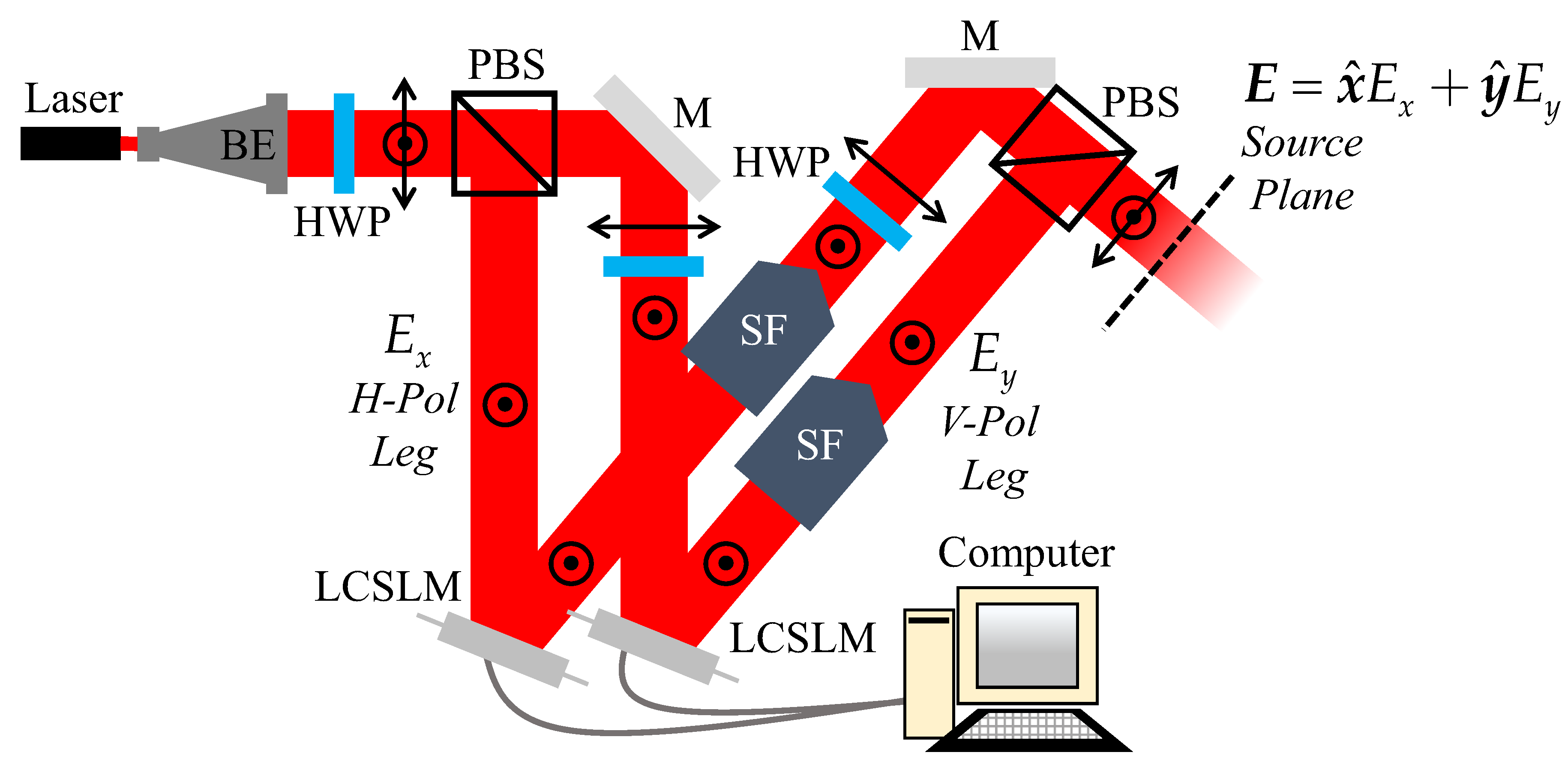
Using the second synthesis method, an electromagnetic PCS can be generated using an apparatus like that in Figure 1. We note that there are variants of this design in the literature, e.g., setups that use a single SLM, use SLMs of different type, or operate on a different basis polarization (circular versus linear states) [7,51,52,53,54,55,56,57,58]. All function using the same basic principle, namely, independent control of the two basis polarization components.

We begin at the laser in Figure 1—light from which passes through a half-wave plate (HWP) followed by a polarizing beam splitter (PBS). The HWP-PBS combination serves to coarsely adjust the power between the horizontal ($E_x$) and vertical ($E_y$) legs of the apparatus (here, we assume a linear basis).

After being split into orthogonal linear components, the light is incident on SLMs—assumed to be liquid crystal (LC) SLMs. Since LCSLMs function by modulating the index ellipsoid of a uniaxial material, they can control polarized light only in a particular state (here, the vertical state) [59,60]. This explains the HWP before the SLM in the $E_y$ leg.

SLMs (depicted as reflective SLMs in Figure 1) commonly modulate light by acting as phase gratings that produce the desired fields in the gratings’ first diffraction orders [61]. For this reason, both the $E_x$ and $E_y$ legs contain spatial filters (SFs) that pass the first diffraction orders and block the others.

Lastly, the light in both legs is recombined in the final PBS—the HWP in the $E_x$ leg is required for this to happen. A field realization is formed at a plane somewhere beyond the final PBS. The location of that plane ultimately depends on the focal lengths of the lenses in the SFs.

Beginning in the next section, we develop the second synthesis method and show that it is capable of generating any physically realizable electromagnetic PCS. Modeling each field’s vector component as a deterministic function (corresponding to the component’s shape) multiplied by a random screen (related to the SLM commands), we derive expressions (superposition integrals) for the $E_x$ and $E_y$ screens that yield electric field realizations consistent with the $\mathbf{W}$ of a desired electromagnetic PCS. Using this analysis, we develop a step-by-step procedure, or recipe, for generating the aforementioned screens from matrices of zero-mean, unit-variance Gaussian random numbers.

To validate our work, we simulate the apparatus in Figure 1 to generate field realizations of a new electromagnetic PCS. From these realizations, we compute planar cuts through the four-dimensional (4D) elements of $\mathbf{W}$ and compare those results to the corresponding theory. Lastly, we conclude with a brief summary of our work and key findings.

2. Materials and Methods

Our analysis begins with the necessary and sufficient criterion for a genuine CSD matrix $\mathbf{W}$ [32,33], namely,

$$\mathbf{W}\left({\rho }_1,{\rho }_2\right)=\int {\int }_{-\infty }^{\infty }\mathbf{H}\left({\rho }_1,\mathit{v}\right)\mathbf{p}\left(\mathit{v}\right){\mathbf{H}}^{†}\left({\rho }_2,\mathit{v}\right){\mathrm{d}}^{2}v,$$

(4)

where $\mathit{v}=\widehat{\mathit{x}}{v}_x+\widehat{\mathit{y}}{v}_y$. The symbol $\mathbf{p}$ in Equation (4) is

$$\begin{array}{c}\mathbf{p}\left(\mathit{v}\right)=\left[\begin{array}{cc}{p}_{xx}\left(\mathit{v}\right)& p_{xy}\left(\mathit{v}\right)\\ p_{xy}^{*}\left(\mathit{v}\right)& p_{yy}\left(\mathit{v}\right)\end{array}\right],\end{array}$$

(5)

where $p_{xx}\left(\mathit{v}\right)\ge 0$, $p_{yy}\left(\mathit{v}\right)\ge 0$, and $p_{xx}\left(\mathit{v}\right)p_{yy}\left(\mathit{v}\right)-{\left|p_{xy}\left(\mathit{v}\right)\right|}^2\ge 0$$\forall \mathit{v}\in {\mathbb{R}}^2$. Lastly, $\mathbf{H}$ is

$$\begin{array}{c}\mathbf{H}\left(\rho ,\mathit{v}\right)=\left[\begin{array}{cc}{H}_x\left(\rho ,\mathit{v}\right)& 0\\ 0& H_y\left(\rho ,\mathit{v}\right)\end{array}\right],\end{array}$$

(6)

where $H_x$ and $H_y$ are arbitrary kernels.

As noted in reference [32], Equation (4) provides a recipe for synthesizing electromagnetic PCSs. Generalizing the scalar case [62], a vector PCS with an arbitrary $\mathbf{W}$ can, in principle, be generated by passing a spatially incoherent field with a polarization matrix $\mathbf{p}$ through two linear optical systems. The transfer functions of those systems, which are generally space-variant (or shift-variant) and operate on the field’s $E_x$ and $E_y$ vector components, are given by $H_x$ and $H_y$, respectively.

For an arbitrary $\mathbf{W}$, it is not likely that the required $H_x$ and $H_y$ are optically realizable. A notable exception is electromagnetic Schell-model sources, where $H_x$ and $H_y$ are Fourier kernels and can easily be realized using spherical lenses—this generally explains their popularity (see above references). Other transfer functions that can be realized physically are Fresnel and Mellin kernels [63].

To synthesize a general electromagnetic PCS, e.g., an electromagnetic nonuniformly correlated beam [15,24,64], we must generate random $E_x$ and $E_y$ realizations, where we perform the filtering (evaluate superposition integrals) numerically. The $E_x$ and $E_y$ realizations are then physically generated using a coherent light source and SLMs (see Figure 1). The electromagnetic PCS is formed from the incoherent addition of many such realizations.

It is important to note that electromagnetic PCSs synthesized in this manner are not produced in real time. This stands in contrast to the approach discussed in reference [32]. Unfortunately, this is the price of flexibility.

We desire to produce random optical field realizations of the form

$$\begin{array}{c}\mathit{E}\left(\rho \right)=\widehat{\mathit{x}}{E}_x\left(\rho \right)+\widehat{\mathit{y}}{E}_y\left(\rho \right)=\widehat{\mathit{x}}{\tau }_x\left(\rho \right)T_x\left(\rho \right)+\widehat{\mathit{y}}{\tau }_y\left(\rho \right)T_y\left(\rho \right),\end{array}$$

(7)

where ${\tau }_x$ and ${\tau }_y$ are deterministic complex functions (physically, the $E_x$ and $E_y$ shapes), and $T_x$ and $T_y$ are circular complex Gaussian screens. Taking the vector auto-correlation of $\mathit{E}$ and comparing the result to Equation (4) produces

$$\begin{array}{c}{\tau }_{\alpha }\left({\rho }_1\right){\tau }_{\beta }^{*}\left({\rho }_2\right)\langle T_{\alpha }\left({\rho }_1\right)T_{\beta }^{*}\left({\rho }_2\right)\rangle =\int {\int }_{-\infty }^{\infty }{p}_{\alpha \beta }\left(\mathit{v}\right)H_{\alpha }\left({\rho }_1,\mathit{v}\right)H_{\beta }^{*}\left({\rho }_2,\mathit{v}\right){\mathrm{d}}^{2}v,\end{array}$$

(8)

where $\alpha ,\beta =x,y$. We let $H_{\alpha }\left(\rho ,\mathit{v}\right)={\tau }_{\alpha }\left(\rho \right)h_{\alpha }\left(\rho ,\mathit{v}\right)$, which simplifies Equation (8) to

$$\begin{array}{c}\langle T_{\alpha }\left({\rho }_1\right)T_{\beta }^{*}\left({\rho }_2\right)\rangle =\int {\int }_{-\infty }^{\infty }{p}_{\alpha \beta }\left(\mathit{v}\right)h_{\alpha }\left({\rho }_1,\mathit{v}\right)h_{\beta }^{*}\left({\rho }_2,\mathit{v}\right){\mathrm{d}}^{2}v.\end{array}$$

(9)

Since the diagonal $\mathbf{W}$ elements, i.e., $W_{xx}$ and $W_{yy}$, can be isolated from an arbitrary $\mathbf{W}$ simply by passing the source through a horizontal or vertical linear polarizer, both $W_{xx}$ and $W_{yy}$ must satisfy the necessary and sufficient criterion for scalar CSD functions [33,62]. Therefore, we can use the recently derived scalar result to produce $T_{\alpha }$ with spatial statistics consistent with $W_{\alpha \alpha }$ [50], namely,

$$\begin{array}{c}{T}_{\alpha }\left(\rho \right)=\int {\int }_{-\infty }^{\infty }{r}_{\alpha }\left(\mathit{v}\right){\left[\frac{1}{2}{p}_{\alpha \alpha }\left(\mathit{v}\right)\right]}^{1/2}{h}_{\alpha }\left(\rho ,\mathit{v}\right){\mathrm{d}}^{2}v,\end{array}$$

(10)

where $r_{\alpha }$ is a delta-correlated, complex, Gaussian random function. Note that $\langle r_{\alpha }\left({\mathit{v}}_1\right)r_{\alpha }^{*}\left({\mathit{v}}_2\right)\rangle =2\delta \left({\mathit{v}}_1-{\mathit{v}}_2\right)$, where $\delta$ is the Dirac delta function.

Evaluating Equation (10) results in $T_{\alpha }$, that when multiplied by ${\tau }_{\alpha }$, produce scalar fields whose ensemble-averaged auto-correlation equals $W_{\alpha \alpha }$. This handles the diagonal elements of $\mathbf{W}$. To control the off-diagonal elements, we need to examine the cross-correlation of $E_x$ and $E_y$, or equivalently via Equations (8) and (9), the cross-correlation of $T_x$ and $T_y$.

Using Equation (10), we take the cross-correlation of $T_x$ and $T_y$, namely,

$$\begin{array}{c}\langle T_x\left({\rho }_1\right)T_y^{*}\left({\rho }_2\right)\rangle =\int \int \int {\int }_{-\infty }^{\infty }\langle r_x\left({\mathit{v}}_1\right)r_y^{*}\left({\mathit{v}}_2\right)\rangle \frac{1}{2}{\left[p_{xx}\left({\mathit{v}}_1\right)p_{yy}\left({\mathit{v}}_2\right)\right]}^{1/2}\hfill \\ \times h_x\left({\rho }_1,{\mathit{v}}_1\right)h_y^{*}\left({\rho }_2,{\mathit{v}}_2\right){\mathrm{d}}^2{v}_1{\mathrm{d}}^2{v}_2\hfill \end{array}.$$

(11)

This expression must equal Equation (9) with $\alpha =x$ and $\beta =y$. This implies that $\langle r_x\left({\mathit{v}}_1\right)r_y^{*}\left({\mathit{v}}_2\right)\rangle =2\left[R^{\mathrm{r}}\left({\mathit{v}}_1\right)+\mathrm{j}{R}^{\mathrm{i}}\left({\mathit{v}}_1\right)\right]\delta \left({\mathit{v}}_1-{\mathit{v}}_2\right)$, where $R^{\mathrm{r}}$ and $R^{\mathrm{i}}$ are the real and imaginary parts of the correlation coefficient between $r_x$ and $r_y$, respectively. Substituting this expression in for $\langle r_x\left({\mathit{v}}_1\right)r_y^{*}\left({\mathit{v}}_2\right)\rangle$ and evaluating the integrals over ${\mathit{v}}_2$ produces

$$\langle T_x\left({\rho }_1\right)T_y^{*}\left({\rho }_2\right)\rangle =\int {\int }_{-\infty }^{\infty }\left[R^{\mathrm{r}}\left(\mathit{v}\right)+\mathrm{j}{R}^{\mathrm{i}}\left(\mathit{v}\right)\right]{\left[p_{xx}\left(\mathit{v}\right)p_{yy}\left(\mathit{v}\right)\right]}^{1/2}{h}_x\left({\rho }_1,\mathit{v}\right)h_y^{*}\left({\rho }_2,\mathit{v}\right){\mathrm{d}}^{2}v,$$

(12)

from which we deduce

$$p_{xy}\left(\mathit{v}\right)=\left[R^{\mathrm{r}}\left(\mathit{v}\right)+\mathrm{j}{R}^{\mathrm{i}}\left(\mathit{v}\right)\right]{\left[p_{xx}\left(\mathit{v}\right)p_{yy}\left(\mathit{v}\right)\right]}^{1/2}.$$

(13)

Here, we are interested in generating electromagnetic PCSs, and therefore, it is more convenient to express Equation (13) as a function of the complex correlation coefficient in terms of $p_{xy}$. Expanding $p_{xy}$ into real and imaginary parts and then inverting Equation (13) produces

$$\begin{array}{c}{R}^{\mathrm{r}}\left(\mathit{v}\right)=p_{xy}^{\mathrm{r}}\left(\mathit{v}\right){\left[p_{xx}\left(\mathit{v}\right)p_{yy}\left(\mathit{v}\right)\right]}^{-1/2}\\ R^{\mathrm{i}}\left(\mathit{v}\right)=p_{xy}^{\mathrm{i}}\left(\mathit{v}\right){\left[p_{xx}\left(\mathit{v}\right)p_{yy}\left(\mathit{v}\right)\right]}^{-1/2}\end{array}.$$

(14)

Since $R^{\mathrm{r}}$ and $R^{\mathrm{i}}$ are correlation coefficients, they must satisfy $\left|R^{\mathrm{r}}\left(\mathit{v}\right)\right|\le 1$ and $\left|R^{\mathrm{i}}\left(\mathit{v}\right)\right|\le 1$$\forall \mathit{v}\in {\mathbb{R}}^2$. It is important to check that this is indeed the case.

Recall the conditions on the elements of $\mathbf{p}$ given below Equation (5). Using the $p_{xy}$ inequality and $p_{xx},p_{yy}\ge 0$, we easily derive $\left|p_{xy}\right|{\left(p_{xx}{p}_{yy}\right)}^{-1/2}\le 1$. This inequality along with the expressions in Equation (14) clearly imply that $-1\le R^{\mathrm{r}},R^{\mathrm{i}}\le 1$. The fact that the conditions on $R^{\mathrm{r}}$ and $R^{\mathrm{i}}$ are consistent with the physics-based stipulations on $\mathbf{p}$, and further, that Equation (4) forms the basis of the $T_x$ and $T_y$ superposition integrals, means that the synthesis approach we present here is capable of producing any electromagnetic PCS with a genuine $\mathbf{W}$.

We conclude this section with a summary of the above analysis. A stochastic optical field realization drawn from a random vector process with second-order moments equal to $\mathbf{W}$ can be generated in the following manner:

• Identify ${\tau }_x$, ${\tau }_y$, $h_x$, $h_y$, $p_{xx}$, $p_{yy}$, and $p_{xy}$ associated with the desired $\mathbf{W}$.
• Compute $R^{\mathrm{r}}$ and $R^{\mathrm{i}}$ using Equation (14).
• Generate $r_x$ and $r_y$. The means of $r_x$ and $r_y$ are zero, and the covariance matrix $\mathsf{\Sigma }$ is

  $$\mathsf{\Sigma }=\left[\begin{array}{cccc}\langle {\left(r_x^{\mathrm{r}}\right)}^2\rangle & \langle r_x^{\mathrm{r}}{r}_x^{\mathrm{i}}\rangle & \langle r_x^{\mathrm{r}}{r}_y^{\mathrm{r}}\rangle & \langle r_x^{\mathrm{r}}{r}_y^{\mathrm{i}}\rangle \\ \langle r_x^{\mathrm{i}}{r}_x^{\mathrm{r}}\rangle & \langle {\left(r_x^{\mathrm{i}}\right)}^2\rangle & \langle r_x^{\mathrm{i}}{r}_y^{\mathrm{r}}\rangle & \langle r_x^{\mathrm{i}}{r}_y^{\mathrm{i}}\rangle \\ \langle r_y^{\mathrm{r}}{r}_x^{\mathrm{r}}\rangle & \langle r_y^{\mathrm{r}}{r}_x^{\mathrm{i}}\rangle & \langle {\left(r_y^{\mathrm{r}}\right)}^2\rangle & \langle r_y^{\mathrm{r}}{r}_y^{\mathrm{i}}\rangle \\ \langle r_y^{\mathrm{i}}{r}_x^{\mathrm{r}}\rangle & \langle r_y^{\mathrm{i}}{r}_x^{\mathrm{i}}\rangle & \langle r_y^{\mathrm{i}}{r}_y^{\mathrm{r}}\rangle & \langle {\left(r_y^{\mathrm{i}}\right)}^2\rangle \end{array}\right]=\left[\begin{array}{cccc}1& 0& R^{\mathrm{r}}& -R^{\mathrm{i}}\\ 0& 1& R^{\mathrm{i}}& R^{\mathrm{r}}\\ R^{\mathrm{r}}& R^{\mathrm{i}}& 1& 0\\ -R^{\mathrm{i}}& R^{\mathrm{i}}& 0& 1\end{array}\right].$$

  (15)
  Using the Cholesky factor [65] of $\mathsf{\Sigma }$, i.e., $\mathsf{\Sigma }=\mathbf{L}{\mathbf{L}}^{\mathrm{T}}$ and

  $$\mathbf{L}=\left[\begin{array}{cccc}1& 0& 0& 0\\ 0& 1& 0& 0\\ R^{\mathrm{r}}& R^{\mathrm{i}}& \sqrt{1-{\left(R^{\mathrm{r}}\right)}^2-{\left(R^{\mathrm{i}}\right)}^2}& 0\\ -R^{\mathrm{i}}& R^{\mathrm{i}}& 0& \sqrt{1-{\left(R^{\mathrm{r}}\right)}^2-{\left(R^{\mathrm{i}}\right)}^2}\end{array}\right],$$

  (16)

  we generate $r_x$ and $r_y$ using the following relations:

  $$\begin{array}{cc}\hfill r_x\left(\mathit{v}\right)& =r_1\left(\mathit{v}\right)+\mathrm{j}{r}_2\left(\mathit{v}\right)\hfill \\ \hfill r_y\left(\mathit{v}\right)& =r_x\left(\mathit{v}\right)\left[R^{\mathrm{r}}\left(\mathit{v}\right)-\mathrm{j}{R}^{\mathrm{i}}\left(\mathit{v}\right)\right]+\sqrt{1-{\left[R^{\mathrm{r}}\left(\mathit{v}\right)\right]}^2-{\left[R^{\mathrm{i}}\left(\mathit{v}\right)\right]}^2}\left[r_3\left(\mathit{v}\right)+\mathrm{j}{r}_4\left(\mathit{v}\right)\right]\hfill \end{array},$$

  (17)

  where $r_1$, $r_2$, $r_3$, and $r_4$ are mutually-independent, delta-correlated, Gaussian random functions.
• Generate $T_x$ and $T_y$ using Equation (10). Since Equation (10) is evaluated numerically, we express it in discrete form for the reader’s convenience:

  $$T_{\alpha }\left[i,j\right]=\sum _m\sum _n{r}_{\alpha }\left[m,n\right]{\left(\frac{1}{2}{p}_{\alpha \alpha }\left[m\Delta v_x,n\Delta v_y\right]\right)}^{1/2}{h}_{\alpha }\left[i\Delta x,j\Delta y,m\Delta v_x,n\Delta v_y\right]\sqrt{\Delta v_x\Delta v_y},$$

  (18)

  where $\Delta x$, $\Delta y$, $\Delta v_x$, and $\Delta v_y$ are the grid spacings in the x-y and $v_x$-$v_y$ planes, respectively. Note that Equation (18) is equivalent to a matrix-vector product.
• Create a field realization $\mathit{E}$ using Equation (7).

In the above analysis, we specify that $r_{\alpha }$ and subsequently $T_{\alpha }$ are Gaussian distributed. Mathematically, $r_{\alpha }$ could be any statistical distribution (“Any statistical distribution” must consider the means and covariances in Equation (15). For instance, textbook exponential, gamma, or Rayleigh random numbers cannot be used to seed $r_{\alpha }$ because their means never equal zero) (uniform, for instance) as long as the means and covariances equal those in Equation (15). This is easy to do, in practice, using linear combinations of independent, normal random numbers [see Equation (17)]. Note that this is not the case for random numbers of other distributions.

Besides convenience, there is also a physical reason to use Gaussian random numbers. The stochastic fields emitted by natural, thermal light sources are known, classically speaking, to be Gaussian distributed [66]. By using normal random numbers to seed $r_{\alpha }$, our field realizations will have the same statistical distribution as natural light.

3. Results and Discussion

Here, we simulate the apparatus in Figure 1 to generate an electromagnetic Gaussian pseudo-Schell-model (EGPSM) source. Before discussing the details of the simulation, we present some background on EGPSM sources.

Pseudo-Schell-model (PSM) sources were first presented in reference [67]. A PSM source differs from a Schell-model source in that its degree of coherence [2,5,66] depends on the radial distance between two points, vice their vector difference. To date, all PSM-source references discuss scalar PSM beams. Here, we generalize those works by creating an electromagnetic PSM source to validate our synthesis method.

The CSD matrix elements of an EGPSM beam are

$$W_{\alpha \beta }\left({\rho }_1,{\rho }_2\right)=A_{\alpha }exp\left(-\frac{{\rho }_1^2}{4{\sigma }_{\alpha }^2}\right)A_{\beta }exp\left(-\frac{{\rho }_2^2}{4{\sigma }_{\beta }^2}\right)B_{\alpha \beta }exp\left[-\frac{{\left({\rho }_1-{\rho }_2\right)}^2}{2{\delta }_{\alpha \beta }^2}\right],$$

(19)

where $A_{\alpha }$ and ${\sigma }_{\alpha }$ are the amplitude and root-mean-square width of the $\alpha$ field component, respectively. In Equation (19), $B_{\alpha \beta }$ is the complex correlation coefficient between the $\alpha$ and $\beta$ field components, and ${\delta }_{\alpha \beta }$ is related to the width of the cross-correlation function. The $H_{\alpha }$ and $p_{\alpha \beta }$ that when substituted into Equation (4) produce Equation (19) are

$$\begin{array}{cc}\hfill H_{\alpha }\left(\rho ,\mathit{v}\right)& ={\tau }_{\alpha }\left(\rho \right)h\left(\rho ,\mathit{v}\right)=A_{\alpha }exp\left(-\frac{{\rho }^2}{4{\sigma }_{\alpha }^2}\right)exp\left(\mathrm{j}\rho vcos\psi \right)\hfill \\ \hfill p_{\alpha \beta }\left(\mathit{v}\right)& =B_{\alpha \beta }\frac{{\delta }_{\alpha \beta }^2}{2\pi }exp\left(-\frac{1}{2}{\delta }_{\alpha \beta }^2{v}^2\right)\hfill \end{array},$$

(20)

where v and $\psi$ are the magnitude and angle of $\mathit{v}$. In addition, $B_{\alpha \beta }$ and ${\delta }_{\alpha \beta }$ must satisfy

$$\begin{array}{c}{B}_{xx}=B_{yy}=1,B_{xy}=B_{yx}^{*},\left|B_{xy}\right|\le 1,{\delta }_{xy}={\delta }_{yx},\\ \sqrt{\frac{{\delta }_{xx}^2+{\delta }_{yy}^2}{2}}\le {\delta }_{xy}\le \sqrt{\frac{{\delta }_{xx}{\delta }_{yy}}{\left|B_{xy}\right|}}\end{array}$$

(21)

for the EGPSM source to be physically realizable or genuine.

Having discussed the EGPSM source, we now turn to the simulation. Because our purpose here is solely a proof-of-concept, our simulation models an idealized version of the apparatus in Figure 1, i.e., perfect HWPs, Ms, PBSs, SFs, and LCSLMs. When using actual or physical SLMs (whether they be liquid crystal, deformable mirrors, or digital micromirrors), pixel pitch, active-area size, fill factor, and phase discretization or digitization all play roles in the quality of the synthesized field realizations. These SLM characteristics and their effects on beam control have been discussed before (please see Refs. [26,45,58,59,61] for more information). The MATLAB^® version R2018b scripts (.m files) are included as Supplementary Materials to this paper.

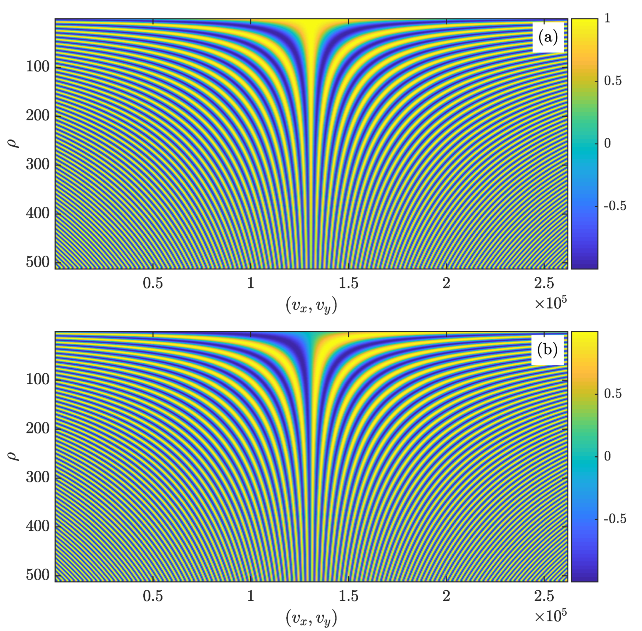
In the simulation, we use $N_x=N_y=512$ points per side grids with spacings in the x-y and $v_x$-$v_y$ planes equal to $\Delta x=\Delta y=0.333\mathrm{mm}$ and $\Delta v_x=\Delta v_y=5.86{\mathrm{m}}^{-1}$, respectively. Note that the transfer functions $h_{\alpha }$ ($N_x{N}_y\times N_x{N}_y$ matrices) are, in general, not spatially band-limited. Representing them discretely is therefore a challenge, and the best we can achieve is to ensure that $h_{\alpha }$ satisfy the Nyquist-Shannon criterion over regions in which $p_{\alpha \alpha }$ and $\left|{\tau }_{\alpha }\right|$ have significant value. As a result, $h_{\alpha }$ are typically large matrices, and thus, require a computer with large amounts of memory to store. Because of the form of h in Equation (20), we can reduce its dimensionality by evaluating h at unique one-dimensional (1D) values of $\rho ={\left(x^2+y^2\right)}^{1/2}$, vice every combination of x and y. Therefore, in the simulation, h is $512\times {512}^2$, where the spacing in the $\rho$ dimension is $\Delta \rho =0.4723\mathrm{mm}$. This $\Delta \rho$, as well as the $\Delta v_x$ and $\Delta v_y$ specified above, are sufficient to accurately represent the EGPSM h without aliasing over the simulated region of interest. Figure 2 shows the real and imaginary parts of the simulated h.

We synthesize $E_x$ and $E_y$ realizations in the following manner:

• Generate four ${512}^2\times 1$ vectors of mutually-independent, zero-mean, unit-variance Gaussian random numbers, i.e., $r_1$, $r_2$, $r_3$, and $r_4$.
• Produce $r_x$ and $r_y$ using item 1 and Equation (17), where $R^{\mathrm{r}}$ and $R^{\mathrm{i}}$ are represented as ${512}^2\times 1$ vectors.
• Multiply (element-wise) $r_{\alpha }$ by $\sqrt{p_{\alpha \alpha }\Delta v_x\Delta v_y/2}$ (represented as ${512}^2\times 1$ vectors).
• Compute the matrix-vector products of h [see Equation (20) and Figure 2] and item 3 to produce $T_{\alpha }$ ($512\times 1$ vectors).
• Interpolate $512\times 1$ vectors $T_{\alpha }$ (discrete functions of $\rho$) to $512\times 512$ matrices $T_{\alpha }$ (2D discrete functions of $x,y$).
• Multiply (element-wise) $T_{\alpha }$ by ${\tau }_{\alpha }$ to form $E_{\alpha }$ realizations.

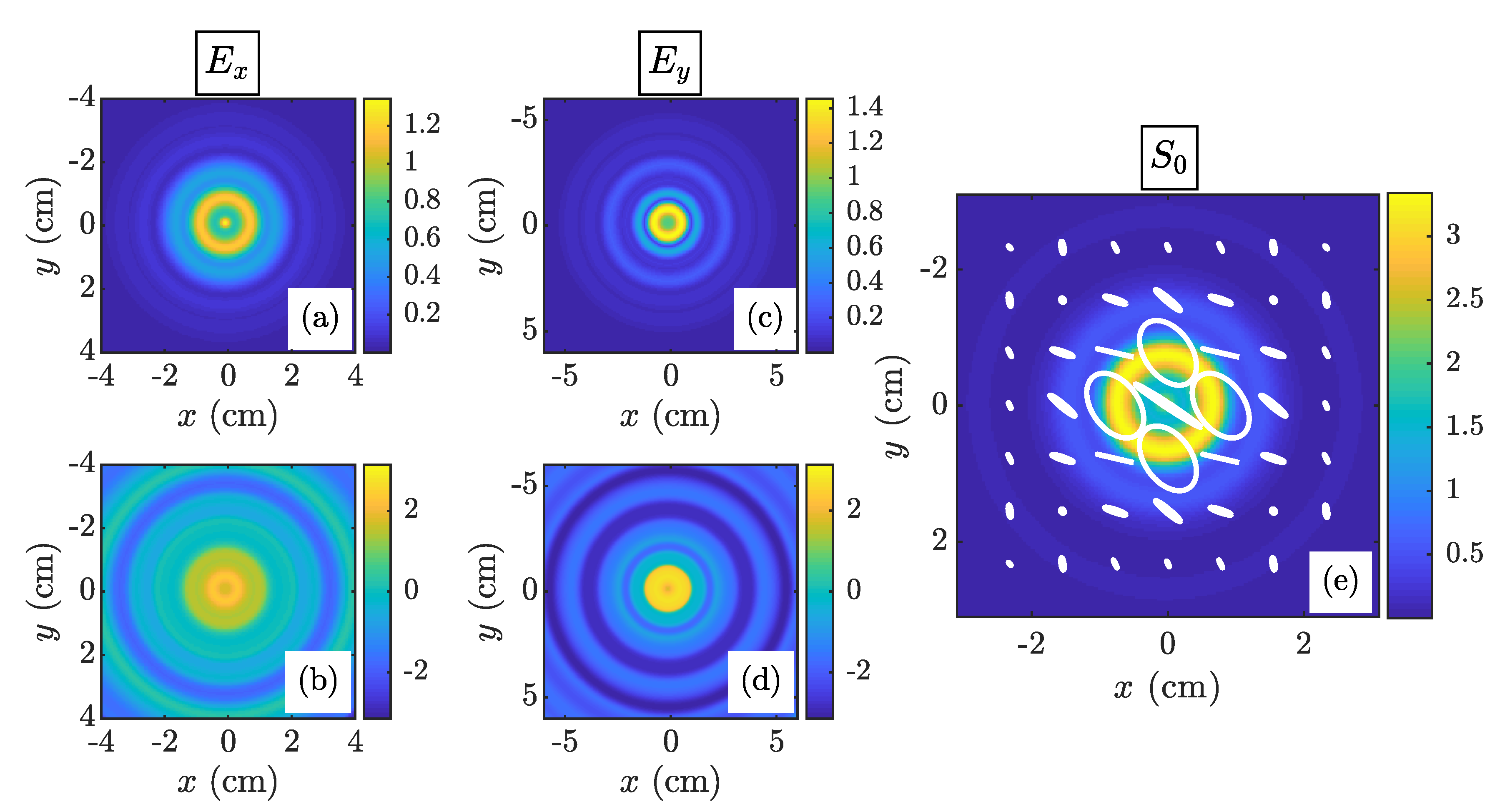
To give the reader insight into the characteristics of EGPSM field realizations, Figure 3 shows $E_x$ and $E_y$ instances generated using the above procedure and the EGPSM source parameters in

Table 1. Simulated EGPSM Source Parameters.

$A_x$	1.25
$A_y$	1
${\sigma }_x$	1 cm
${\sigma }_y$	1.25 cm
$B_{xy}$	0.5 $exp\left(-\mathrm{j}\pi /5\right)$
${\delta }_{xx}$	3.33 mm
${\delta }_{yy}$	4.17 mm
${\delta }_{xy}$	5.12 mm

: (a) and (b) show $\left|E_x\right|$ and $arg\left(E_x\right)$, respectively; (c) and (d) show the same for $E_y$. Lastly, (e) shows the “instantaneous” intensity, or $S_0={\left|E_x\right|}^2+{\left|E_y\right|}^2$, overlaid by the polarization ellipses [see Equation (3)] computed at several locations across the beam’s profile.

To verify that indeed the $E_x$ and $E_y$ instances depicted in Figure 3 are representative of the ensemble of all EGPSM field realizations, we compute the Stokes parameters [see Equation (2)] and $\mathbf{W}\left(x_1,0,x_2,0\right)$ from 10,000 independent $E_x$ and $E_y$ realizations. We then compare the simulated results to theory, which we compute using Equation (19) and Table 1.

The Stokes parameter results are shown in Figure 4. The figure is organized as follows: The images in column 1—i.e, (a), (c), (e), and (g)—show $S_0$, $S_1$, $S_2$, and $S_3$ theory (superscript “thy” in the caption and “Thy” column heading); column 2 [(b), (d), (f), and (h)] shows $S_0$, $S_1$, $S_2$, and $S_3$ simulation (superscript “sim” in the caption and “Sim” column heading). The theoretical and simulated Stokes parameters are plotted on the same false color scales defined by the bars immediately adjacent to column 2. Column 3 shows larger views of $S_0^{\mathrm{thy}}$ and $S_0^{\mathrm{sim}}$—(j) and (k), respectively—both overlaid with the polarization ellipses at 81 different locations across the EGPSM beam’s profile. Lastly, (i) shows the 2D correlation coefficients of the theoretical and simulated Stokes parameters plotted versus field realization (random trial) number. The inset shows a close up view of the correlation coefficients from trials 100 to 10,000.

The agreement between the simulated and theoretical results in Figure 4 is excellent. These results imply that our synthesis method produces a beam with the desired (correct) shape and polarization state. Further, Figure 4i shows that our method does so in roughly 500–600 field realizations—the simulated Stokes parameters are at least 99% similar to their theoretical counterparts.

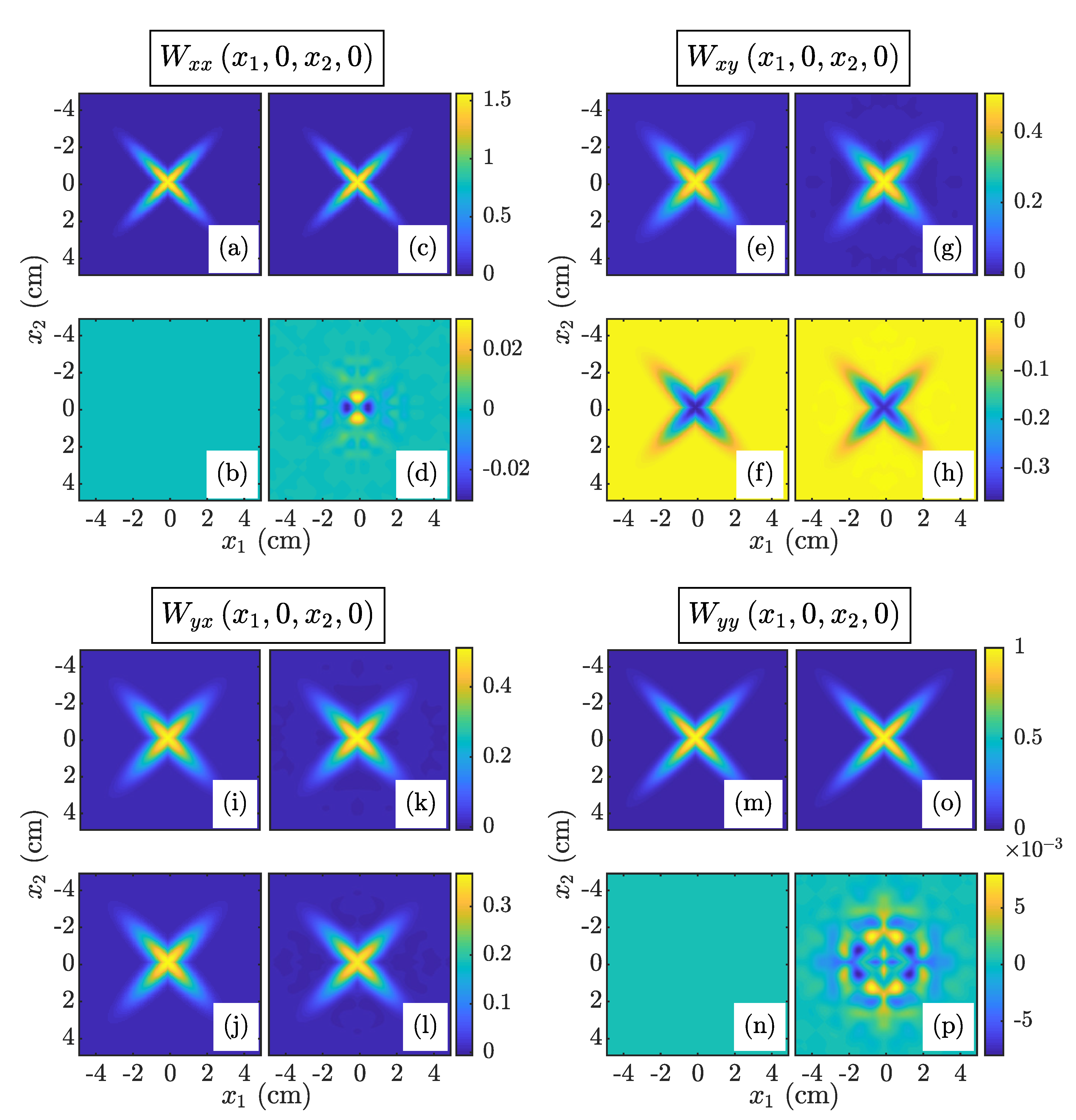
As previously stated, the quality of the results in Figure 4 shows quite definitively that our method produces a beam with the proper shape and polarization characteristics. To verify that our method produces a beam with the correct spatial correlation or coherence properties, we need to examine the CSD matrix elements. Since each CSD matrix element is a 4D function, a 2D planar slice through that hyperspace must suffice for validation purposes.

Figure 5 shows the theoretical and simulated $\mathbf{W}\left(x_1,0,x_2,0\right)$. The figure is organized to mimic the layout of the $2\times 2$ CSD matrix $\mathbf{W}$. Each $\mathbf{W}$ “element”—labeled for the reader’s convenience—consists of a $2\times 2$ block of images. All blocks are arranged in the same way—theory is in column 1, simulation is in column 2, real parts are in row 1, and imaginary parts are in row 2. For instance, the $2\times 2$ block corresponding to $W_{xx}$ (the upper left-hand block) shows the real and imaginary parts of $W_{xx}^{\mathrm{thy}}$ in (a) and (b), respectively. The same results for $W_{xx}^{\mathrm{sim}}$ are shown in (c) and (d), respectively. The real and imaginary parts of $W_{xx}^{\mathrm{thy}}$ and $W_{xx}^{\mathrm{sim}}$ are plotted on the same false color scales defined by the bars at each row’s end.

The agreement between the theoretical and simulated CSD matrix elements in Figure 5 is excellent. Note that the conspicuous discrepancies between $W_{xx}^{\mathrm{thy}}$ and $W_{xx}^{\mathrm{sim}}$ imaginary [(b) and (d)] and $W_{yy}^{\mathrm{thy}}$ and $W_{yy}^{\mathrm{sim}}$ imaginary [(n) and (p)] are, in fact, quantitatively small, being approximately 100 and 200 times smaller than their associated real parts, respectively. Both of these discrepancies are due to the fact that the imaginary parts of $W_{xx}^{\mathrm{thy}}$ and $W_{yy}^{\mathrm{thy}}$ are identically zero. To match those values in simulation, would require an infinite number of field realizations.

The excellent quality of the results in Figure 5 implies that our method is producing a beam with the correct, or desired spatial correlation properties. When combined with the excellent results in Figure 4, we can claim that we successfully produced the desired EGPSM source.

4. Conclusions

In this paper, we developed a method to generate any physically realizable, or genuine electromagnetic PCS. Starting with the necessary and sufficient criterion for genuine CSD matrices, we derived integral expressions for two stochastic screens (associated with the field’s vector components) that, when multiplied by the components’ deterministic shapes, produced a desired electromagnetic PCS field realization. To aid the reader, we summarized our analysis by presenting a step-by-step recipe for synthesizing the aforementioned screens from matrices of zero-mean, unit-variance, independent Gaussian random numbers.

We validated our synthesis approach by generating (in simulation) field realizations of an EGPSM beam—a new electromagnetic PCS. From 10,000 EGPSM field realizations, we computed the Stokes parameters and planar cuts through the CSD matrix elements. We compared these results to the corresponding theoretical quantities to verify we produced a beam with the desired shape, polarization, and coherence properties.

The simulated EGPSM results were found to be in excellent agreement with theory. In addition, we found that the simulated results converged to their theoretical counterparts in approximately 500–600 field realizations. This finding will be useful to optical scientists who are considering utilizing this approach for a particular application.

In conclusion, we note that the method presented here can be implemented on existing SLM-based vector beam generators with no additional hardware. Also, it can be used in any application which utilizes vector partially coherent beams. These include, but are not limited to, optical tweezers, medicine, directed energy, and remote sensing.

References

- Wolf, E. Unified theory of coherence and polarization of random electromagnetic beams. Phys. Lett. A 2003, 312, 263–267. [Google Scholar] [CrossRef]
- Mandel, L.; Wolf, E. Optical Coherence and Quantum Optics; Cambridge University: New York, NY, USA, 1995. [Google Scholar]
- Wolf, E. Introduction to the Theory of Coherence and Polarization of Light; Cambridge University: Cambridge, UK, 2007. [Google Scholar]
- Agarwal, G.S.; Classen, A. Partial coherence in modern optics: Emil Wolf’s legacy in the 21st century. Prog. Opt. 2019. [Google Scholar] [CrossRef] [Green Version]
- Korotkova, O. Random Light Beams: Theory and Applications; CRC: Boca Raton, FL, USA, 2014. [Google Scholar]
- Gbur, G. Partially coherent beam propagation in atmospheric turbulence. J. Opt. Soc. Am. A 2014, 31, 2038–2045. [Google Scholar] [CrossRef] [PubMed] [Green Version]
- Zhan, Q. (Ed.) Vectorial Optical Fields: Fundamentals and Applications; World Scientific: Hackensack, NJ, USA, 2014. [Google Scholar]
- Efimov, A. Gigabit per second modulation and transmission of a partially coherent beam through laboratory turbulence. Proc. SPIE 2016, 9739, 163–168. [Google Scholar] [CrossRef]
- Korotkova, O. Light propagation in a turbulent ocean. Prog. Opt. 2019, 64, 1–43. [Google Scholar] [CrossRef]
- Korotkova, O.; Gbur, G. Applications of optical coherence theory. Prog. Opt. 2020. [Google Scholar] [CrossRef]
- Borghi, R.; Gori, F.; Ponomarenko, S.A. On a class of electromagnetic diffraction-free beams. J. Opt. Soc. Am. A 2009, 26, 2275–2281. [Google Scholar] [CrossRef]
- Cai, Y.; Chen, Y.; Wang, F. Generation and propagation of partially coherent beams with nonconventional correlation functions: A review. J. Opt. Soc. Am. A 2014, 31, 2083–2096. [Google Scholar] [CrossRef]
- Voelz, D.; Xiao, X.; Korotkova, O. Numerical modeling of Schell-model beams with arbitrary far-field patterns. Opt. Lett. 2015, 40, 352–355. [Google Scholar] [CrossRef]
- Hyde, M.W.; Basu, S.; Voelz, D.G.; Xiao, X. Experimentally generating any desired partially coherent Schell-model source using phase-only control. J. Appl. Phys. 2015, 118, 093102. [Google Scholar] [CrossRef] [Green Version]
- Lajunen, H.; Saastamoinen, T. Propagation characteristics of partially coherent beams with spatially varying correlations. Opt. Lett. 2011, 36, 4104–4106. [Google Scholar] [CrossRef] [PubMed]
- Santarsiero, M.; Martínez-Herrero, R.; Maluenda, D.; de Sande, J.C.G.; Piquero, G.; Gori, F. Partially coherent sources with circular coherence. Opt. Lett. 2017, 42, 1512–1515. [Google Scholar] [CrossRef] [PubMed] [Green Version]
- Piquero, G.; Santarsiero, M.; Martínez-Herrero, R.; de Sande, J.C.G.; Alonzo, M.; Gori, F. Partially coherent sources with radial coherence. Opt. Lett. 2018, 43, 2376–2379. [Google Scholar] [CrossRef]
- Yu, J.; Cai, Y.; Gbur, G. Rectangular Hermite non-uniformly correlated beams and its propagation properties. Opt. Express 2018, 26, 27894–27906. [Google Scholar] [CrossRef] [PubMed]
- Mei, Z.; Korotkova, O. Random sources for rotating spectral densities. Opt. Lett. 2017, 42, 255–258. [Google Scholar] [CrossRef]
- Hyde, M.W. Generating electromagnetic Schell-model sources using complex screens with spatially varying auto- and cross-correlation functions. Results Phys. 2019, 15, 102663. [Google Scholar] [CrossRef]
- Mei, Z.; Korotkova, O. Electromagnetic Schell-model sources generating far fields with stable and flexible concentric rings profiles. Opt. Express 2016, 24, 5572–5583. [Google Scholar] [CrossRef] [PubMed]
- Liang, C.; Mi, C.; Wang, F.; Zhao, C.; Cai, Y.; Ponomarenko, S.A. Vector optical coherence lattices generating controllable far-field beam profiles. Opt. Express 2017, 25, 9872–9885. [Google Scholar] [CrossRef] [PubMed]
- Chen, Y.; Wang, F.; Yu, J.; Liu, L.; Cai, Y. Vector Hermite-Gaussian correlated Schell-model beam. Opt. Express 2016, 24, 15232–15250. [Google Scholar] [CrossRef] [PubMed]
- Tong, Z.; Korotkova, O. Electromagnetic nonuniformly correlated beams. J. Opt. Soc. Am. A 2012, 29, 2154–2158. [Google Scholar] [CrossRef] [PubMed]
- Ostrovsky, A.S.; Olvera, M.A.; Rickenstorff, C.; Martínez-Niconoff, G.; Arrizón, V. Generation of a secondary electromagnetic source with desired statistical properties. Opt. Commun. 2010, 283, 4490–4493. [Google Scholar] [CrossRef]
- Hyde, M.W.; Bose-Pillai, S.; Voelz, D.G.; Xiao, X. Generation of vector partially coherent optical sources using phase-only spatial light modulators. Phys. Rev. Appl. 2016, 6, 064030. [Google Scholar] [CrossRef] [Green Version]
- Hyde, M.W. Shaping the far-zone intensity, degree of polarization, angle of polarization, and ellipticity angle using vector Schell-model sources. Results Phys. 2019, 12, 2242–2250. [Google Scholar] [CrossRef]
- Mei, Z.; Korotkova, O.; Shchepakina, E. Electromagnetic multi-Gaussian Schell-model beams. J. Opt. 2013, 15, 025705. [Google Scholar] [CrossRef]
- Mao, H.; Chen, Y.; Liang, C.; Chen, L.; Cai, Y.; Ponomarenko, S.A. Self-steering partially coherent vector beams. Opt. Express 2019, 27, 14353–14368. [Google Scholar] [CrossRef]
- Mao, Y.; Wang, Y.; Mei, Z. Electromagnetic fractional multi-Gaussian Schell-model beams and their statistical properties. J. Opt. 2019, 21, 035601. [Google Scholar] [CrossRef]
- Mishra, S.; Gautam, S.K.; Naik, D.N.; Chen, Z.; Pu, J.; Singh, R.K. Tailoring and analysis of vectorial coherence. J. Opt. 2018, 20, 125605. [Google Scholar] [CrossRef]
- Shirai, T. Interpretation of the recipe for synthesizing genuine cross-spectral density matrices. Opt. Commun. 2010, 283, 4478–4483. [Google Scholar] [CrossRef]
- Gori, F.; Ramírez-Sánchez, V.; Santarsiero, M.; Shirai, T. On genuine cross-spectral density matrices. J. Opt. A Pure Appl. Opt. 2009, 11, 085706. [Google Scholar] [CrossRef]
- Grella, R. Synthesis of generalized Collett-Wolf sources. J. Opt. 1982, 13, 127–131. [Google Scholar] [CrossRef]
- Santarsiero, M.; Borghi, R.; Ramírez-Sánchez, V. Synthesis of electromagnetic Schell-model sources. J. Opt. Soc. Am. A 2009, 26, 1437–1443. [Google Scholar] [CrossRef] [PubMed]
- Hyde, M.W. Controlling the spatial coherence of an optical source using a spatial filter. Appl. Sci. 2018, 8, 1465. [Google Scholar] [CrossRef] [Green Version]
- Cai, Y.; Chen, Y.; Yu, J.; Liu, X.; Liu, L. Generation of partially coherent beams. Prog. Opt. 2017, 62, 157–223. [Google Scholar] [CrossRef]
- Wang, H.; Peng, X.; Liu, L.; Wang, F.; Cai, Y.; Ponomarenko, S.A. Generating bona fide twisted Gaussian Schell-model beams. Opt. Lett. 2019, 44, 3709–3712. [Google Scholar] [CrossRef] [PubMed]
- Friberg, A.T.; Tervonen, E.; Turunen, J. Interpretation and experimental demonstration of twisted Gaussian Schell-model beams. J. Opt. Soc. Am. A 1994, 11, 1818–1826. [Google Scholar] [CrossRef]
- Wang, F.; Liang, C.; Yuan, Y.; Cai, Y. Generalized multi-Gaussian correlated Schell-model beam: From theory to experiment. Opt. Express 2014, 22, 23456–23464. [Google Scholar] [CrossRef]
- Wang, F.; Wu, G.; Liu, X.; Zhu, S.; Cai, Y. Experimental measurement of the beam parameters of an electromagnetic Gaussian Schell-model source. Opt. Lett. 2011, 36, 2722–2724. [Google Scholar] [CrossRef]
- Liu, X.; Wang, F.; Liu, L.; Zhao, C.; Cai, Y. Generation and propagation of an electromagnetic Gaussian Schell-model vortex beam. J. Opt. Soc. Am. A 2015, 32, 2058–2065. [Google Scholar] [CrossRef]
- Piquero, G.; Gori, F.; Romanini, P.; Santarsiero, M.; Borghi, R.; Mondello, A. Synthesis of partially polarized Gaussian Schell-model sources. Opt. Commun. 2002, 208, 9–16. [Google Scholar] [CrossRef]
- Shirai, T.; Korotkova, O.; Wolf, E. A method of generating electromagnetic Gaussian Schell-model beams. J. Opt. A Pure Appl. Opt. 2005, 7, 232–237. [Google Scholar] [CrossRef]
- Hyde, M.W.; Bose-Pillai, S.R.; Wood, R.A. Synthesis of non-uniformly correlated partially coherent sources using a deformable mirror. Appl. Phys. Lett. 2017, 111, 101106. [Google Scholar] [CrossRef] [Green Version]
- Shirai, T.; Wolf, E. Coherence and polarization of electromagnetic beams modulated by random phase screens and their changes on propagation in free space. J. Opt. Soc. Am. A 2004, 21, 1907–1916. [Google Scholar] [CrossRef] [PubMed]
- Ostrovsky, A.S.; Martínez-Niconoff, G.; Arrizón, V.; Martínez-Vara, P.; Olvera-Santamaría, M.A.; Rickenstorff-Parrao, C. Modulation of coherence and polarization using liquid crystal spatial light modulators. Opt. Express 2009, 17, 5257–5264. [Google Scholar] [CrossRef] [PubMed]
- Ostrovsky, A.S.; Rodríguez-Zurita, G.; Meneses-Fabián, C.; Olvera-Santamaría, M.A.; Rickenstorff-Parrao, C. Experimental generating the partially coherent and partially polarized electromagnetic source. Opt. Express 2010, 18, 12864–12871. [Google Scholar] [CrossRef] [PubMed]
- Basu, S.; Hyde, M.W.; Xiao, X.; Voelz, D.G.; Korotkova, O. Computational approaches for generating electromagnetic Gaussian Schell-model sources. Opt. Express 2014, 22, 31691–31707. [Google Scholar] [CrossRef] [PubMed]
- Hyde, M.W. Stochastic complex transmittance screens for synthesizing general partially coherent sources. J. Opt. Soc. Am. A 2020, 37, 257–264. [Google Scholar] [CrossRef] [PubMed]
- Rosales-Guzmán, C.; Ndagano, B.; Forbes, A. A review of complex vector light fields and their applications. J. Opt. 2018, 20, 123001. [Google Scholar] [CrossRef]
- Yu, Z.; Chen, H.; Chen, Z.; Hao, J.; Ding, J. Simultaneous tailoring of complete polarization, amplitude and phase of vector beams. Opt. Commun. 2015, 345, 135–140. [Google Scholar] [CrossRef]
- Chen, Z.; Zeng, T.; Qian, B.; Ding, J. Complete shaping of optical vector beams. Opt. Express 2015, 23, 17701–17710. [Google Scholar] [CrossRef]
- Mitchell, K.J.; Turtaev, S.; Padgett, M.J.; Čižmár, T.; Phillips, D.B. High-speed spatial control of the intensity, phase and polarisation of vector beams using a digital micro-mirror device. Opt. Express 2016, 24, 29269–29282. [Google Scholar] [CrossRef] [Green Version]
- Rosales-Guzmán, C.; Bhebhe, N.; Forbes, A. Simultaneous generation of multiple vector beams on a single SLM. Opt. Express 2017, 25, 25697–25706. [Google Scholar] [CrossRef]
- Rosales-Guzmán, C.; Bhebhe, N.; Mahonisi, N.; Forbes, A. Multiplexing 200 spatial modes with a single hologram. J. Opt. 2017, 19, 113501. [Google Scholar] [CrossRef]
- Fu, S.; Zhai, Y.; Wang, T.; Yin, C.; Gao, C. Tailoring arbitrary hybrid Poincarè beams through a single hologram. Appl. Phys. Lett. 2017, 111, 211101. [Google Scholar] [CrossRef]
- Scholes, S.; Kara, R.; Pinnell, J.; Rodríguez-Fajardo, V.; Forbes, A. Structured light with digital micromirror devices: A guide to best practice. Opt. Eng. 2019, 59, 1–12. [Google Scholar] [CrossRef]
- Restaino, S.R.; Teare, S.W. Introduction to Liquid Crystals for Optical Design and Engineering; SPIE Press: Bellingham, WA, USA, 2015. [Google Scholar]
- Zhang, Z.; You, Z.; Chu, D. Fundamentals of phase-only liquid crystal on silicon (LCOS) devices. Light Sci. Appl. 2014, 3, e213. [Google Scholar] [CrossRef]
- Rosales-Guzmán, C.; Forbes, A. How to Shape Light with Spatial Light Modulators; SPIE Press: Bellingham, WA, USA, 2017. [Google Scholar]
- Gori, F.; Santarsiero, M.; Borghi, R.; Ramírez-Sánchez, V. Realizability condition for electromagnetic Schell-model sources. J. Opt. Soc. Am. A 2008, 25, 1016–1021. [Google Scholar] [CrossRef] [PubMed]
- Goodman, J.W. Introduction to Fourier Optics, 3rd ed.; Roberts & Company: Englewood, CO, USA, 2005. [Google Scholar]
- Hyde, M.W.; Xiao, X.; Voelz, D.G. Generating electromagnetic nonuniformly correlated beams. Opt. Lett. 2019, 44, 5719–5722. [Google Scholar] [CrossRef]
- Watkins, D.S. Fundamentals of Matrix Computations, 2nd ed.; Wiley: New York, NY, USA, 2002. [Google Scholar]
- Goodman, J.W. Statistical Optics, 2nd ed.; Wiley: Hoboken, NJ, USA, 2015. [Google Scholar]
- de Sande, J.C.G.; Martínez-Herrero, R.; Piquero, G.; Santarsiero, M.; Gori, F. Pseudo-Schell model sources. Opt. Express 2019, 27, 3963–3977. [Google Scholar] [CrossRef]
Figure 1.
Schematic of an electromagnetic PCS generator—BE is beam expander, HWP is half-wave plate, PBS is polarizing beam splitter, LCSLM is liquid crystal spatial light modulator, M is mirror, and SF is spatial filter.
Figure 2.
Real and imaginary parts—(a,b), respectively—of the EGPSM h in Equation (20). In the simulation, h is a matrix as shown here.
Figure 3.
EGPSM field realization—(a) , (b) , (c) , (d) , and (e) “instantaneous” overlaid with the polarization ellipses at several locations across the beam’s profile.
Figure 4.
EGPSM Stokes parameter results—(a) , (b) , (c) , (d) , (e) , (f) , (g) , (h) , (i) 2D correlation coefficients of the theoretical and simulated Stokes parameters plotted versus field realization number, (j) overlaid with the polarization ellipses at several locations across the beam’s profile, and (k) overlaid with the polarization ellipses at several locations across the beam’s profile.
Figure 5.
EGPSM results—(a,b) real and imaginary parts of , (c,d) real and imaginary parts of , (e,f) real and imaginary parts of , (g,h) real and imaginary parts of , (i,j) real and imaginary parts of , (k,l) real and imaginary parts of , (m,n) real and imaginary parts of , and (o,p) real and imaginary parts of .