Article

A First Step towards Determining the Ionic Content in Water with an Integrated Optofluidic Chip Based on Near-Infrared Absorption Spectroscopy

1
Wetsus, European Centre of Excellence for Sustainable Water Technology, Oostergoweg 9, 8911 MA Leeuwarden, The Netherlands
2
Optical Sciences Group, University of Twente, Postbus 217, 7500 AE Enschede, The Netherlands
*
Author to whom correspondence should be addressed.
Submission received: 19 June 2020 / Revised: 8 July 2020 / Accepted: 9 July 2020 / Published: 11 July 2020
(This article belongs to the Special Issue Fabrication and Applications of Photonic Micro-Devices)

Abstract

:
In this work, we present a feasibility study of integrated optofluidic chips to measure the ionic content in water using differential absorption spectroscopy. The second overtone of the OH-stretch vibration of water is used as indicator for both the type and concentration of the dissolved ions. The optofluidic chips are based on silicon nitride (TripleX) containing Mach–Zehnder interferometers (MZI) with two 5 cm sensing paths for the sample and reference arms, respectively. Simulations show that, theoretically, the determination of both the type and concentration of a mixture of four electrolytes is possible with the techniques presented. However, the performance of the chips deviated from the expected results due to the insufficient reproducibility and precision in the fabrication process. Therefore, at this early stage, the chips presented here could only determine the ion concentration, but not differentiate between the different ion types. Still, this work represents the first steps towards the realization of an online and real-time sensor of ionic content in water.

1. Introduction

1.1. The Relevance of Detecting Ionic Content in Water

1.1.1. Government Sector

A large variety of dissolved ions (ionic content) are present in drinking water. Some of the ions are essential and beneficial (e.g., Cu2+, Cr3+, and Zn2+) though toxic in excess, while others are toxic in trace amounts (e.g., Pb2+, Hg2+, Cd2+, Tl3+) and have no known biochemical value [1].The adverse effect of consuming unhealthy water is cumulative. For example, between 35 and 77 million people in Bangladesh were poisoned, with 407 deaths, occurring over a period of nine years due to the contamination of groundwater with arsenic compounds [2].
Another toxic contaminant found in drinking water is nitrite; a known risk factor for infant methemoglobinemia—A condition that can cause coma and death if left untreated [3,4].
Guidelines are set by health organizations with knowledge of the impact of different contaminants on health. Improvements in the accuracy of sensors lead to a better understanding of the impact contaminants have on the environment and for human health.
The legislation concerning safe drinking water differs by country. Humanitarian aid organizations provide water treatment equipment and educate local populations in developing countries to ensure a better quality of life with success: in 2015, 91% of the global population had access to improved drinking water sources as compared to the 76% in 1990 [5]. Still, the issue remains that the water may not be safe for consumption due to incorrect equipment operation or maintenance. Cheap sensors integrated into water treatment equipment are needed for widespread quality assurance.
Water-borne illness can occur even in developed and wealthy countries, for example, by chemical spillage from industry, leading to the contamination of drinking water reservoirs [6]. Moreover, the distribution system can be contaminated by tampering and accidental pipeline failures [7,8,9,10].
The presence of accidental contaminants should, however, not be the only concern for those managing drinking water systems; the dangers of bioterrorism have to be considered as well. On-line and real-time sensors play a critical role in the first line of defense [11,12,13].

1.1.2. Industry

Not only the government sector is pushing towards the improvements of sensors but process control in many industrial plants relies on knowing the exact mineral content in process water. The conventional procedure for the identification and quantification of different ions in water is sample collection at discrete intervals of time, which are then sent to specialists in a dedicated lab. The potential saving of resources motivates the industry to spend time and money on the development of innovative sensors.
Potential users can be found in the agricultural, biotechnology, food and beverage, electroplating, environmental analysis, metal processing, mining, power generation, chemistry, pulp and paper, pharmaceutical, and the semiconductor industries.
In this work, integrated optofluidic chips for determining the ionic content in water are presented. First, an introduction of the optical technique and a brief description of the fabricated chips is given. After that, a theoretical model is presented followed by a simulation of a measurement of a solution with four different electrolytes is presented. Finally the performance of the optofluidic chips is tested and compared to the theoretical results.

1.2. Choice of Spectral Region

Nowadays, the standard method for the determination of ionic content is ion chromatography (IC) [14,15,16]. Classical techniques for the detection of ionic content in water include methods such as titration, gravimetry, turbidimetry, colorimetry, and electrochemistry; potentiometry, coulometry, or voltammetry. Many classical lab techniques can be transferred to compact lab-on-a-chip devices thanks to microscale fabrication [17,18]. This is the next logical step for enabling the smart monitoring devices necessary for assuring a safe and compliant water supply.
Several regions of the electromagnetic spectrum can be used for the optical identification of aqueous ions, from infrared (IR) to ultraviolet (UV). For example, ionic identification relying solely on direct light–ion interactions can be achieved with UV light by probing electronic vibrations. However, this method is difficult to realize on a chip, since it would require an exotic material choice to enable the light propagation, and it would require both an expensive light source and detector. Alternatively, the vibrations of polyatomic ions can be observed with IR light [19]. However, again the materials to realize a chip in this energy region, light source and detector are expensive; and this method cannot detect monoatomic ions. Therefore, we have chosen another option: the near-infrared (NIR). In this region, the absorption spectrum of water contains overtones and combinations of the fundamental vibrations of the H2O molecule. The first overtone bands lay in the telecom wavelength region (1260–1675 nm) and can be probed using light sources and detectors made out of Germanium (Ge) or indium gallium arsenide (InGaAs). This region has the advantage of extensive research in aqueous spectroscopy, however, the materials involved—Ge and InGaAs—are expensive. Less studied is the second overtone band of the OH stretch lying between 900 and 1050 nm. The required on-chip path length to achieve the needed sensitivity for this spectral region is roughly 10 cm [20]. The third overtone OH band requires a path length of ~100 cm to achieve a reasonable sensitivity and is therefore impractical. Therefore, the second overtone absorbance band of the OH stretch vibrations was chosen for the present study: Here, different ions induce a unique spectral change in the absorption spectrum with the signal exhibiting a linear dependence (Lambert–Beer law) on the concentration of the ions. The spectral region (940–1040 nm) is suitable for on-chip miniaturization using the TriPleX platform, a silicon nitride core embedded in silicon oxide [20]. TriPleX technology features low losses [21] for the NIR wavelengths required. Finally, for this spectral region, relatively cheap light sources (like, for example, the super luminescent diode (SLD) used in this work) and detectors are available.

1.3. Method of Detection

As explained above, the optical method used in this work utilizes the influence ions have on the OH vibrations of water. Dissolving salt in water induces a small spectral absorption difference of the infrared absorption of water that is specific and linear dependent on the dissolved salt and temperature. In a previous work, we have shown that the second overtone band of the OH stretch can indeed be used to identify and quantify sixteen different inorganic salts dissolved in water [22]. In that work, we also presented two evaluation methods, Gaussian curve fitting and frequency-wise linear regression fitting of difference absorbance spectra [22]. The spectrometer used in that work (UV1800, Shimadzu GmbH, Reinach, Switzerland) allowed a limit of detection (LOD) of ~30 mM.
Furthermore, we showed that the influence radius of the ions (the hydration shell) can be estimated to extend for approximately two layers of water around the investigated ion. Thus, the signals of mixtures of electrolytes yield superimposed spectra as long as the concentration is sufficiently low so that different ions (and their hydration shells) do not strongly interact with each other. Furthermore, the temperature was found to be a key element in suppressing possible non-linear contributions found at higher concentrations.
In order to improve upon the LOD reported previously [22], in this work, we apply the method of direct optical subtraction. Here the absorbance spectrum of water is optically subtracted from the absorbance spectrum of the aqueous electrolyte using interferometry. The differential absorption spectrum is obtained by recording the destructive interference output of an on-chip interferometer, in our case a Mach–Zehnder Interferometer (MZI). The output at destructive interference yields the imbalance between the two arms, thus showing the absorption. The advantage of this method is that the LOD achievable with optical subtraction is inversely proportional to the integration time, in contrast to the LOD achievable with the electronic subtraction, which is determined by the dynamic range of the detector. Naturally, optical subtraction requires a stable π shift difference between the reference and the sample path. Because even very small differences in temperature can affect this shift, we tried to minimize this influence by having both the reference and sample path pass through the same solvent. On the other hand, we used this dependency to compensate the change of the real part of the refractive index due to the ions in water by adding local heaters on our chip using the same design as in Roeloffzen et al. [23], thereby adjusting the effective refractive index of the reference path to achieve destructive interference. The role of temperature as a control parameter has also been investigated in a previous publication [24]. Since we anticipated difficulties in matching the pathlengths over the full spectrum we also designed MZIs with a predetermined pathlength difference. Here, the idea is to fit the spectral output to determine the change in the complex refractive index. The imaginary part of the complex refractive index represents the absorbance but the real part also contains information on the ion type and concentration.
For long absorption lengths, both the sample and reference arm incur considerable absorption, reducing the absolute output signal as well as the difference signal. By again combining the output of the MZI with a local oscillator (LO), additional on-chip interferometery with homodyne amplification was realized.
To avoid confusion between the two types of interference, we chose a large pathlength difference for the local oscillator path.

1.4. Integrated Optofluidic Chips

The integration of the chosen optical method was realized by the design and fabrication of integrated optofluidic chips with the TriPleX technology [20]. Optofluidics is, simply put, the combination of microfluidics and integrated optics generating a compact bypass system. The remote signal and data processing, in situ/in-line capability, being non-intrusive, small and compact are advantages of optofluidic devices that make them suitable candidates for the next high technology-driven sensor for the determination of ionic content in water [25,26].
The first step towards realizing an integrated optofluidic sensor was the development of chips with single mode operation in the spectral region from 940 to 1040 nm. The integrated optofluidic chips tested in this work have been extensively described elsewhere [22] and will only be briefly discussed here for reasons of understanding.
Figure 1A presents a diagram of the optical layout. The input (left) was split in two parts, one part served as the local oscillator. The other arm was split again into a reference arm and a sample arm. The sample arm interacted with the electrolyte solution whereas the reference arm interacted only with the solvent (in our case: water). After the interaction, both arms were combined. Different designs had different pathlength differences between the two arms. In the most basic design, the pathlength difference was kept as small as possible (with a heater to fine tune it) to create destructive interference over the full spectrum. This output was split into two parts, one of which was put directly on a spectrometer. This part is referred to as the MZI output. It directly yielded the absorption difference between the electrolyte and the solution (the differential absorption). Since this signal was very small, the other half was combined with the local oscillator. The local oscillator had a considerable pathlength difference so that many fringes were generated over the full spectrum and the modulation depth seen in the spectrum contained a homodyne amplification of the difference signal. This output is referred to as the homodyne output. The last output channel (split from the local oscillator) was just the input spectrum, used for normalization.
The TripleX technology was used to enable the single mode (TE0) operation in a spectral region from 940 to 1040 nm. The light was guided by a Si3N4 core with a SiO2 cladding (buried waveguide). Etching the top cladding enabled the evanescent field to probe both the reference and sample channel. Based on these principles, thirty integrated optofluidic chips from three different wafers and four different designs were fabricated by LioniX (LioniX international, Enschede, NL) and tested at Wetsus. The basic design consisted of three parts: a power fluctuation monitor of the light source using a bidirectional coupler, a MZI with a 5 cm interaction length in both arms, and a second MZI partly recombined with a LO as shown in Figure 1A.
The geometric path length differences of 0.3, 59.5, 150, and 300 µm between the two arms of the first optical layout were designed to realize 0, 10, 26, and 52 fringes in the bandwidth in the output of the first MZI.
The geometric path length of the local oscillator resulted in an additional modulation of 35, 61, 68, and 61 fringes in the spectra output. The output of the MZI was bisected with a Y junction before recombining with the LO, so that conclusions could be drawn from the relative losses of the sensing and buried waveguides without having to consider the coupling losses. The waveguides were tapered to allow light coupling from a fiber array (FA) to the chip and vice versa. As presented in Figure 2, this FA consisted of three PM fibers (FC/APC, PM780-HP) used for the coupling light from the SLD to the chip and nine SM fibers (FC/PC, 980-HP) used for the coupling light from the chip to the detectors.

2. Simulated Device Performance

This chapter contains a purely theoretical approach to the expected performance of the optofluidic chips. In section A, the physics of an MZI are discussed. Section B presents the simulated results of null depth, fringe spacing and spectral transmission assuming a spectrometer with a resolution of 0.6 nm. In Section C, the experimental results for the different concentrations of Pb(NO3)2 from an earlier work are used to simulate a measurement of these solutions, and a fitting method able to correctly calculate the concentrations of four different electrolytes from a simulated spectrum is presented.

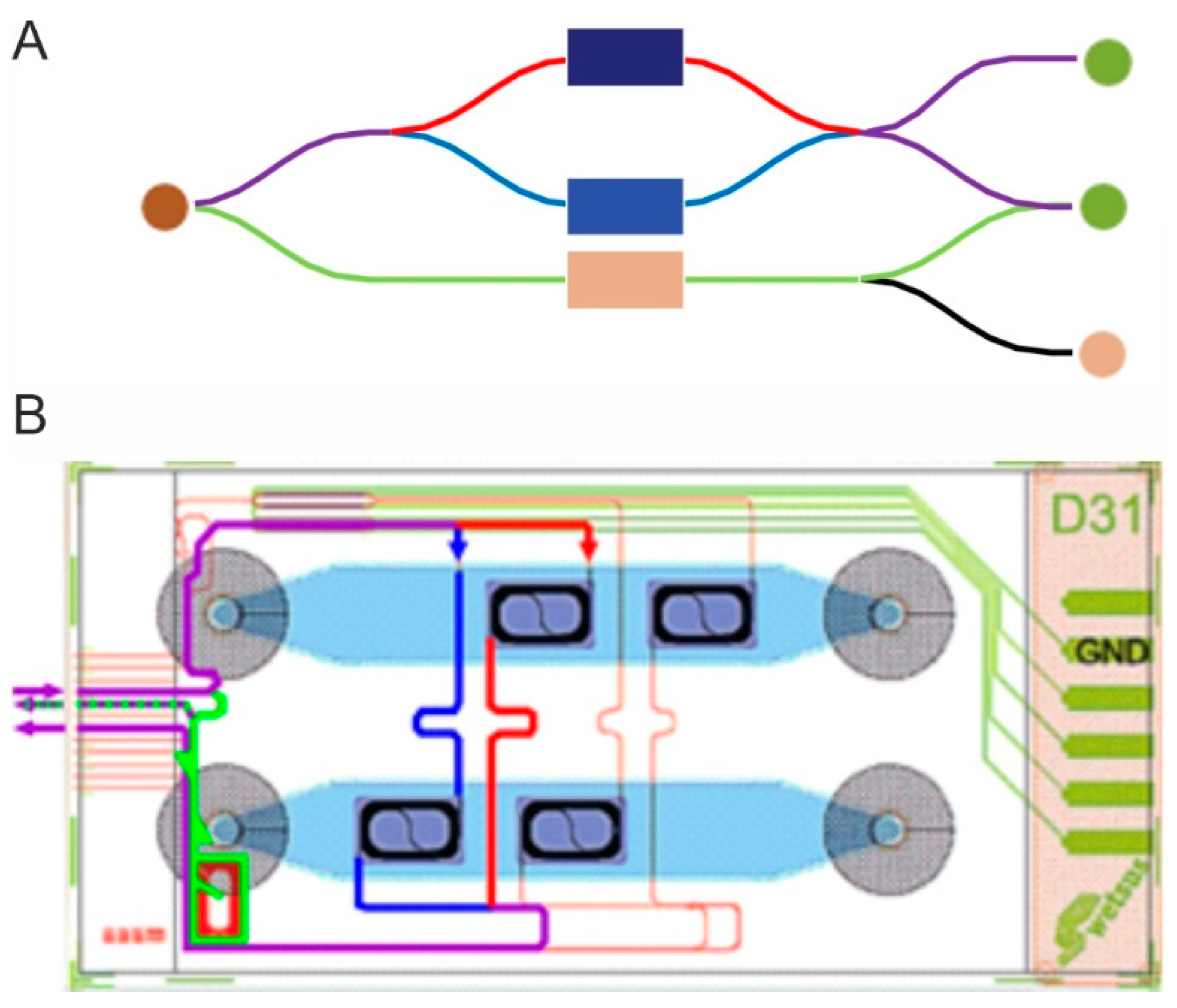
2.1. Mach–Zehnder Interferometer (MZI)

In an MZI, the spectral power density S generated by a light source is first bisected and later recombined by matched optical components. Either free-space (e.g., cube/plate, pellicle, and dichroic beam splitter) or integrated optical components (e.g., Y-splitters, bidirectional-, Ξ- and MMI couplers) can be used to split the light into two co-propagating beams with spectral power densities S0 and S1. One beam probes the sample while the other serves as a reference. The spectral intensity of the recombined light depends on the phase and intensity relation between the two beams. The interference between the two beams at an angular frequency (ω) is expressed by the spectral interference law [27]:
S M Z ( R , Δ M Z , ω ) = S 0 ( R ,   ω ) + S 1 ( R ,   ω ) + 2 S 0 ( R ,   ω ) S 1 ( R ,   ω ) c o s ( ω c Δ M Z ( R ,   ω ) ) ,
where S0 and S1 are the spectral power densities of the sample and the reference beam, respectively. The R in the spectral inference law is the transverse position vector, SMZ is the resultant spectral power density, and ΔMZ is the spatially dependent optical path difference between the two propagating beams at the output of the MZI. The optical power at the output of the MZI can be directly guided by free space components to a device capable of recording the spectral power, or an optical fiber can be used to couple the light from the output of the interferometer to a spectrometer. The effect of a wavelength-dependent aperture function (A(R,λ)) due to the numerical aperture of the fiber and a response function (R(λλ′)) of the spectrometer can be expressed as
I M Z ( Δ M Z , ω ) = S M Z ( R ,   Δ M Z , ω ) A ( R , ω ) R ( ω ω )   d 2 R d ω ,
where IMZ is the resultant intensity of the MZI. Equations (1) and (2) can be combined by assuming the response function of the spectrometer to be a Gaussian function with half-width ΓR, i.e,
R ( ω ω ) = R 0 π Γ R e ( ω ω ) 2 Γ R 2 .
and further assuming the spectral phase (ϕ(ω) = (c/ω) ΔMZ (ω)) can be expanded in a second-order Taylor series:
ϕ ( ω )   ϕ ( ω ) + ϕ ( ω ) ( ω ω ) + 0.5 ϕ ( ω ) ( ω ω ) ,  
and finally assuming the functions S0(R,ω), S1(R,ω) and A(R,ω) to vary slowly with the wavelength:
S M Z ( ω ) = I 0 ( ω ) + I 1 ( ω ) + 2 V A ( ω ) V R ( ω ) I 0 ( ω ) I 1 ( ω ) c o s ( ω c Δ M Z ( ω ) ) = I i n ( ω )   [ 1 + V I ( ω )   c o s ( ϕ R ) ] ,
where I0 and I1 are the intensities of the sample and reference beam, and VA and VR are the spectral visibility terms of the spectral fringes. High visibility (V approaching unity) leads to a nearly 100% fringe modulation. The overall visibility (VI) of the spectral fringes depend on dispersion, the response function of the recording device, the coherence length of the light source and the power imbalance of the beams of the reference and sample arm in the MZI:
VI = VA VR VP VA
is the visibility of the spectral interference fringes at the output of the fiber used to collect the light at one output port of the MZI. It also includes the effect of mode overlap. The visibility due to the power imbalance (VP) and the visibility due to the effect of the limited spectral resolution of a spectrometer (VR) and the spectral phase ϕR is given by
V P = 2 I 0 I 1 I 0 + I 1
and:
V R ( ω ) = 1 1 + σ 2 e 0.25 Γ R 2 ϕ 2 1 1 + σ 2  
and:
ϕ R ( ω ) = ϕ ( ω ) + 0.25 Γ R 2 ϕ 2 ( ω ) σ ( ω ) 1 + σ 2 ( ω ) 0.5 a r c t a n ( σ ( ω ) ) = ϕ ( ω ) .
By neglecting the second order dispersion σ = 0.5 Γ R 2 ϕ ( ω ) it follows that:
V R ( ω ) = e 0.25 Γ R 2 ϕ 2
and:
ϕ R ( ω ) = ϕ ( ω ) .
From ΔλR = Δλ’R 2 and Δλ’R = λ2 ΓR/(2 π c) it follows that:
Γ R 2 = 2 ( π c ) 2 ( Δ λ R / λ 2 ) 2 .
The final expression for the spectral intensity of a MZI is obtained by combining Equations (5), (7)–(9):
S M Z ( ω ) = I i n [ 1 + V A V P ( ω ) e 0.25 Γ R 2 σ 2 c o s ( ω c Δ M Z ( ω ) ) ] S M Z ( λ ) = I i n [ 1 + V A V P ( λ ) e 0.5 ( π Δ λ R Δ M Z g ) 2 / λ 4 c o s ( 2 π λ Δ M Z ( λ ) ) ] .

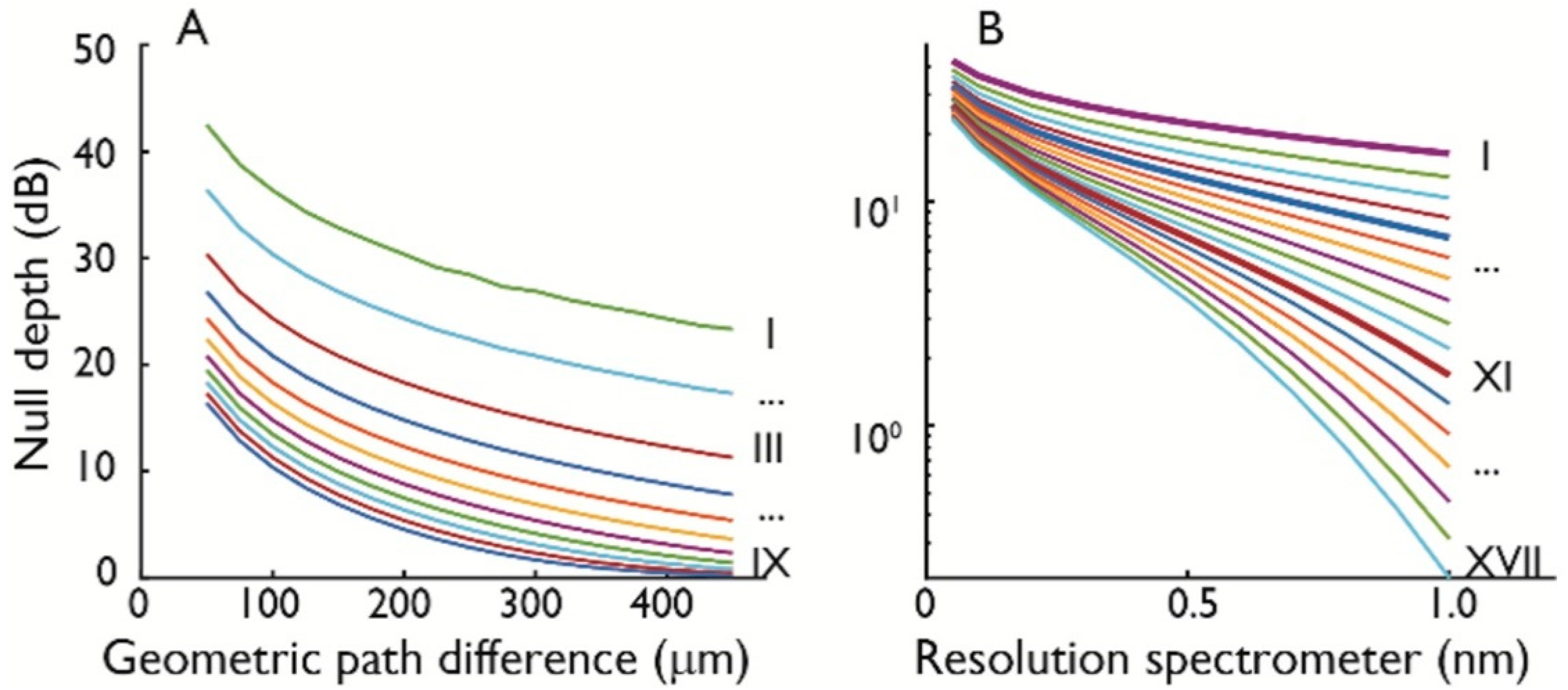
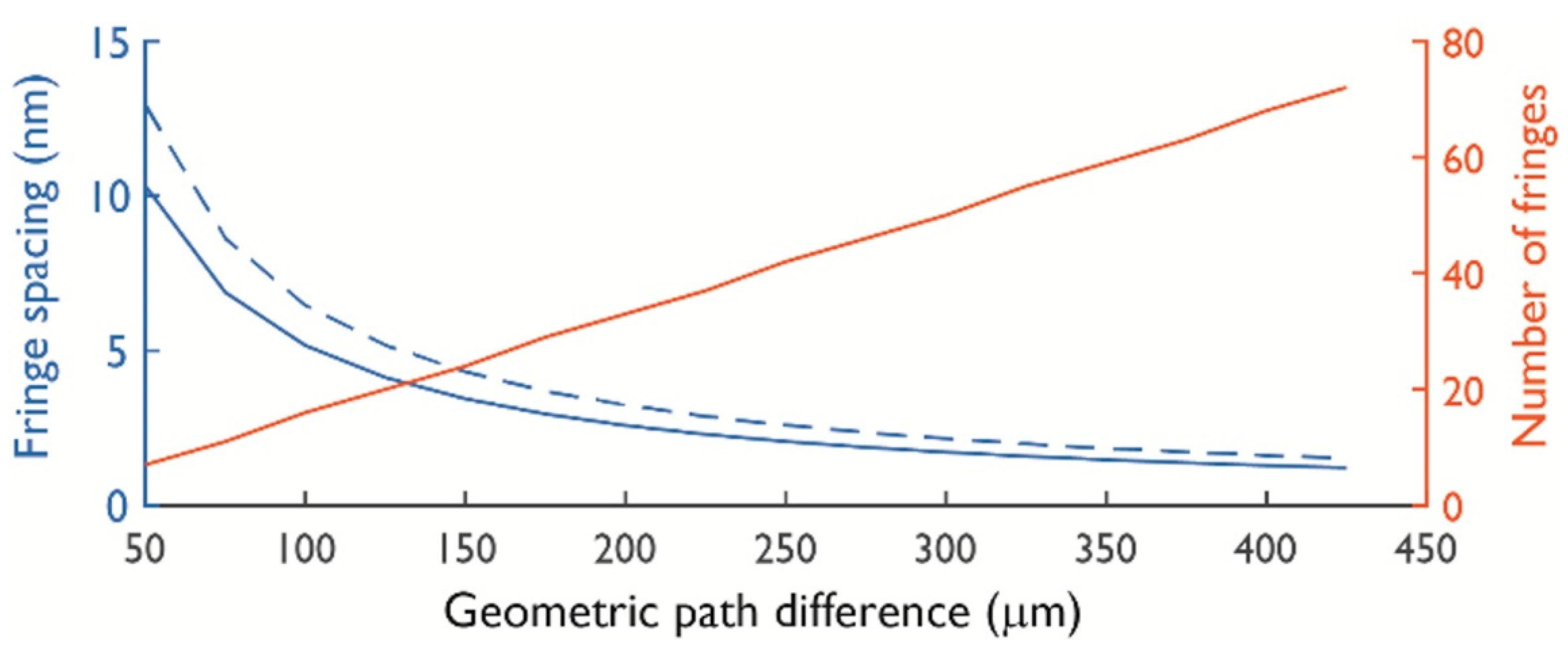
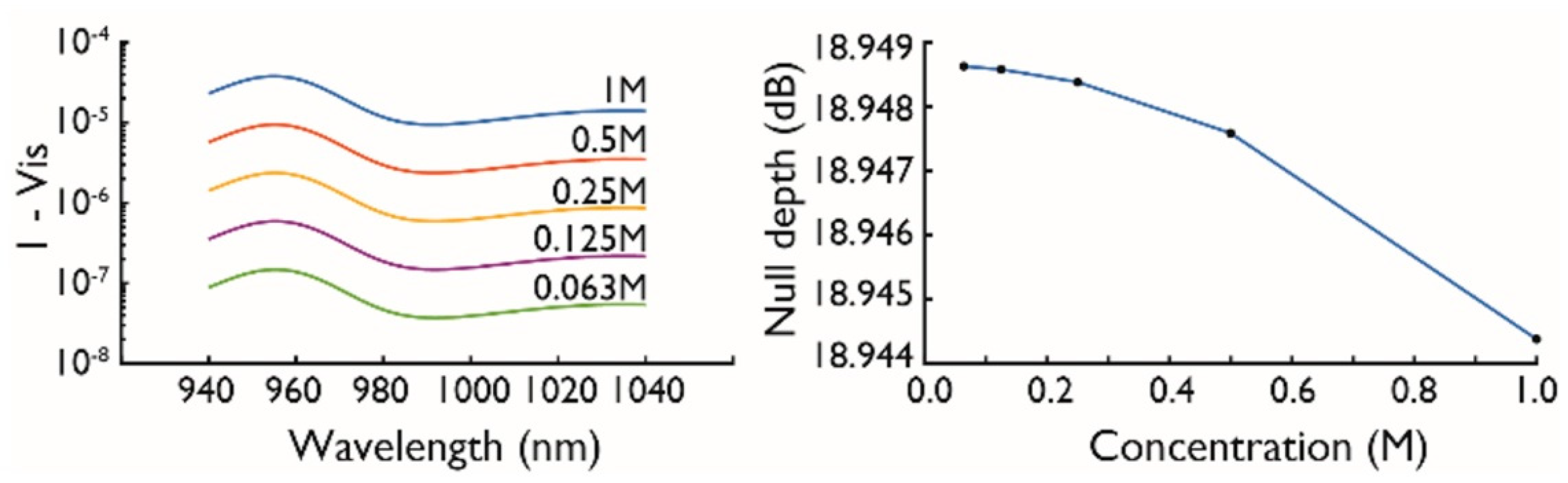
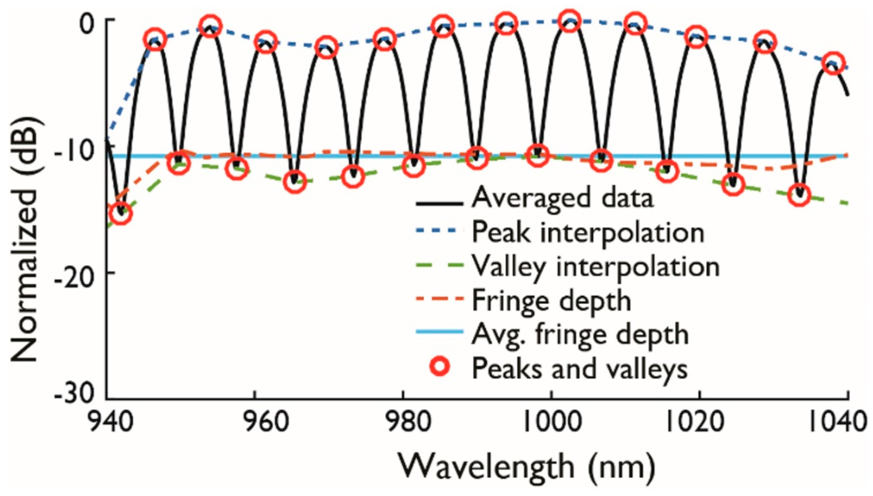
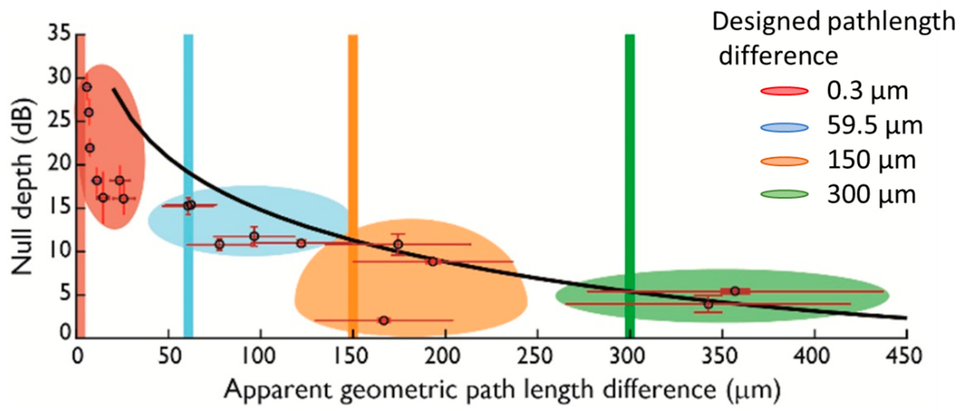
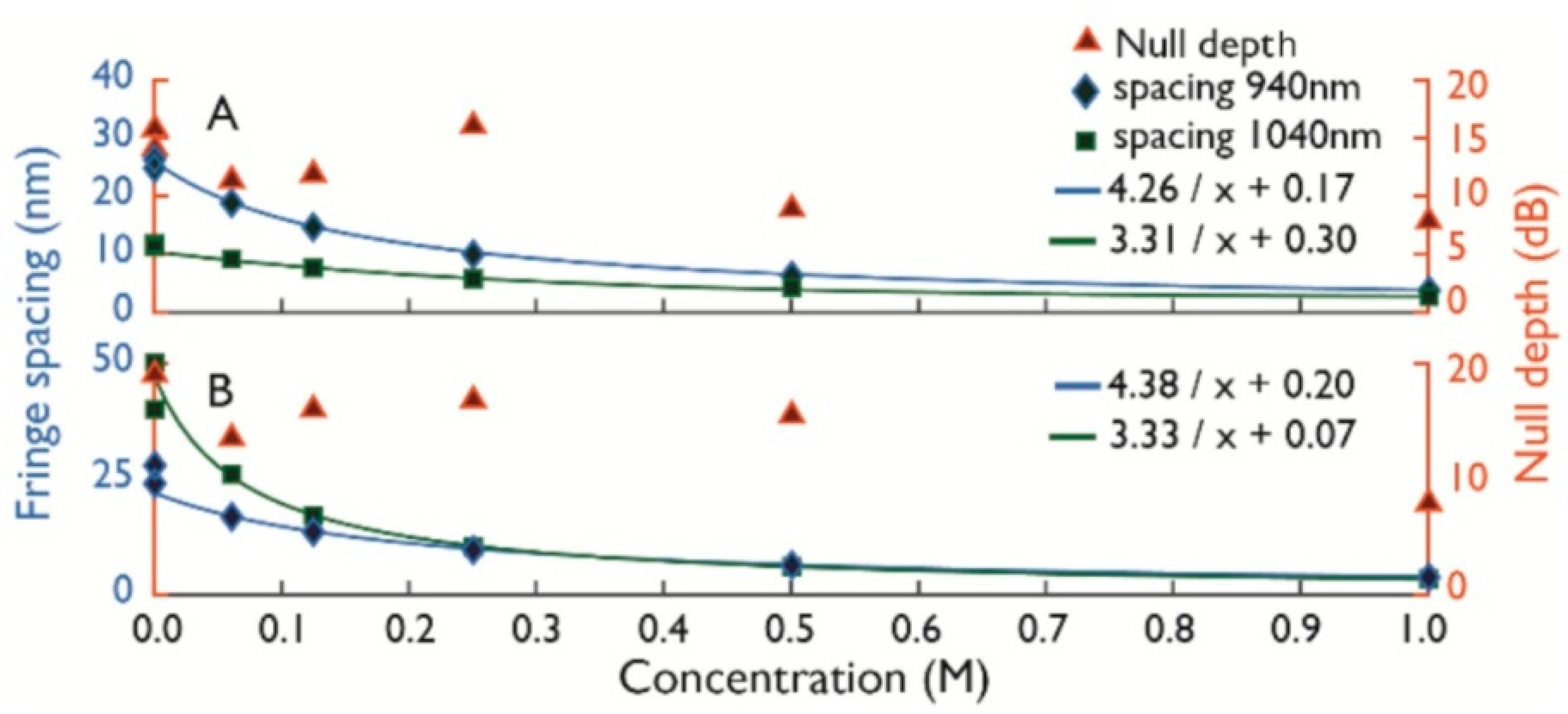
2.2. Null Depth and Fringe Spacing

Equation (13) was implemented in a MATLAB script (R2017b, the MathWorks, Natick, MA, USA) to determine the spectral transmission of a spectrometer with a resolution of 0.6 nm and a data interval of 10 pm for eight optical path differences (0.30, 0.31, 0.32, 0.33, 0.34, 59.5, 150, and 300 µm). The calculations were performed using the effective refractive index (λ dependent) of the designed cross-section of the buried waveguides. A recorded spectrum of an SLD was normalized and used for Iin, and the visibility terms were set to one. The expected transmission spectra for the different geometrical path differences are presented in Figure 2.
The use of continuous spectrum in combination with a finite resolution on the spectrometer causes the null depth (i.e., the full magnitude of the fringe modulation) to degrade for larger path length differences (and the corresponding narrower fringe spacing). Additional calculations were performed and presented in Figure 3 to also show the influence of the spectral resolution (of the recording device) and the path difference between the two arms. A data interval of 4 pm was used. A deeper null depth can be expected if the fringes can be resolved with the recording device.
The spectral fringe spacing increases almost linearly with the wavelength for a fixed geometric path difference, showing a dispersion of −1251 ps/(nm·km). This number was calculated from two linear regression fits on the fringe spacing at 940 and 1040 nm for different geometric path differences in our chip design. The result from the MATLAB calculation is presented in Figure 4. The fringe spacing Ls determined for the geometric path difference (Lgeo in nm) can be described with (Ls = 516,500/Lgeo) and (Ls = 647,200/Lgeo) for the wavelength at 940 and 1040 nm, respectively.

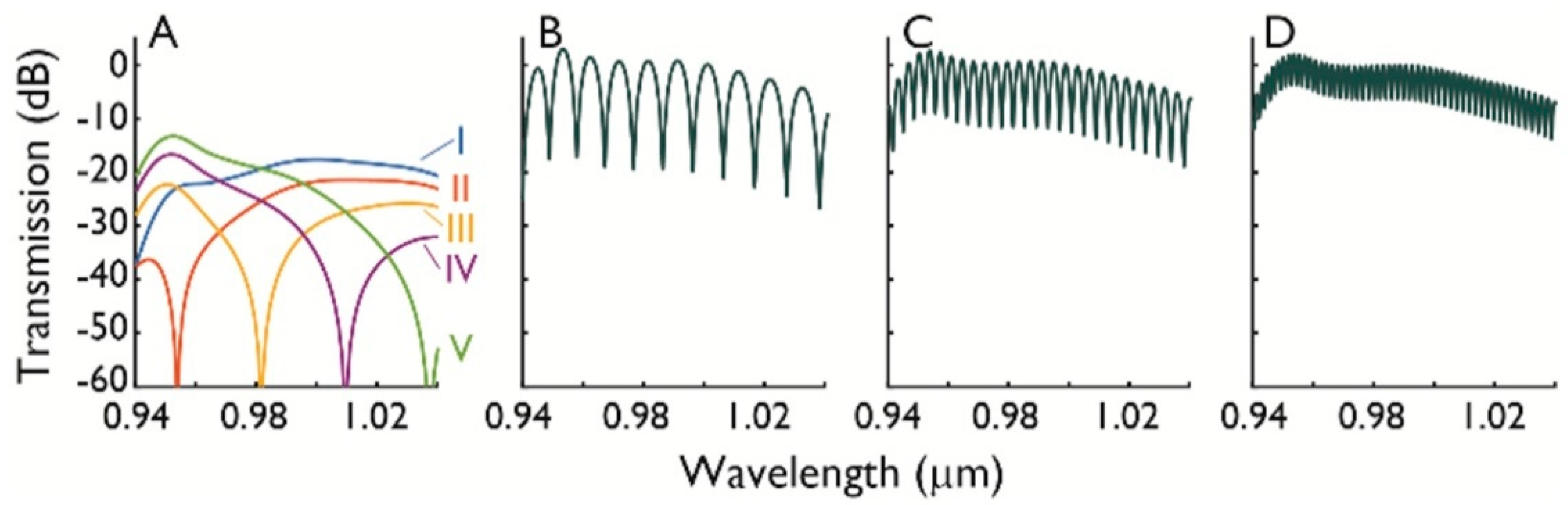
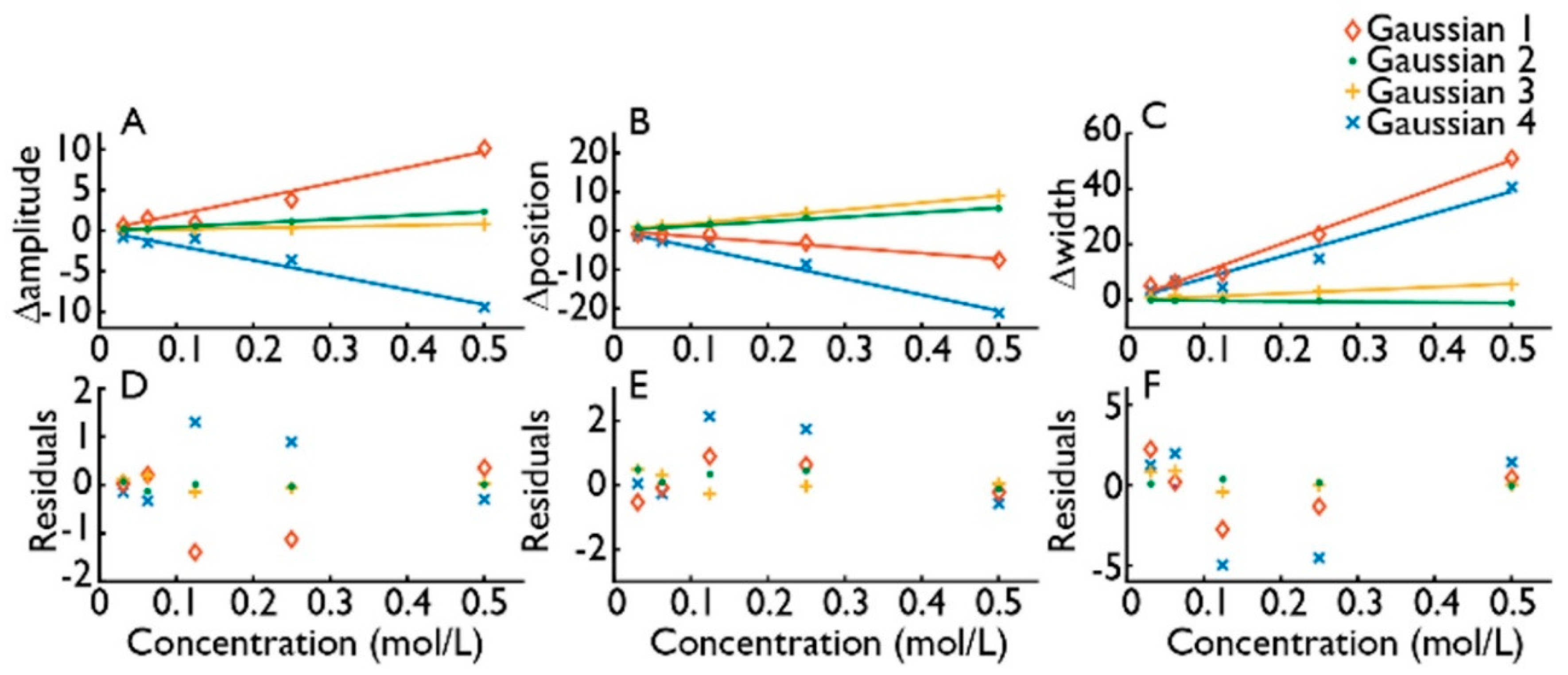
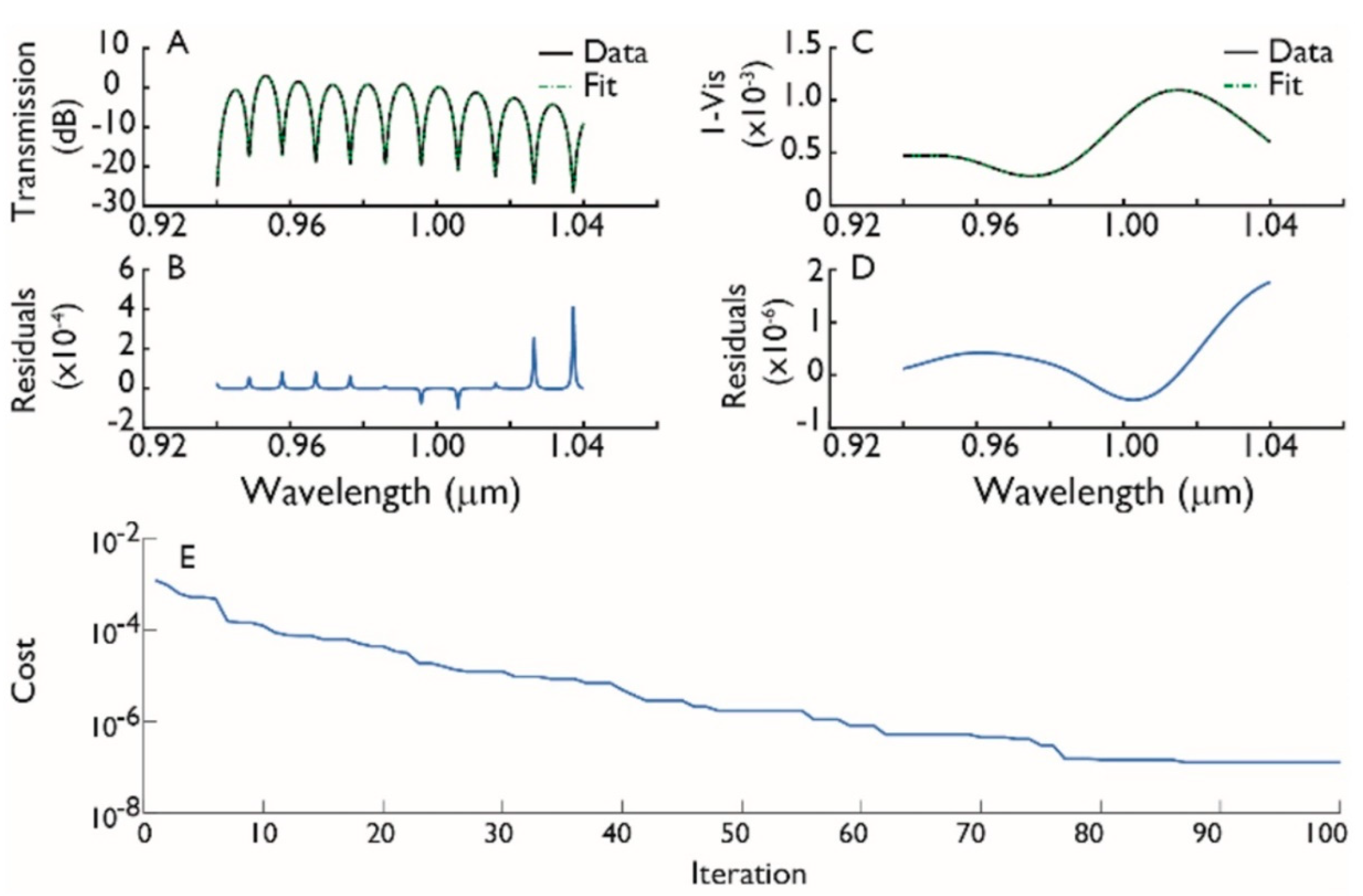
2.3. Differential Absorbance

In a previous work, we have shown that the changes of the second OH stretch vibration overtone of water, induced by the addition of ions, can be successfully analyzed by applying a Gaussian curve fitting method. [22]. In this method, we showed that three parameters—amplitude, position and width—of four distinct Gaussian curves (thus 12 parameters in total) could be used to unambiguously identify 16 electrolytes at different concentrations. The differential absorbance spectra of these electrolytes were published in an earlier work (see Figure 4 of ref. [22]). Of course, the spectrum of pure water without ionic content can be similarly described by four Gaussian curves. Therefore, the differential absorbance, which can be considered the fingerprint of the ionic content in the NIR region, can be also be represented with four Gaussians. In Figure 5, we use the experimental parameters of different concentrations of Pb(NO3)2 from a previous work [22] in order to show their (almost) linear dependence on concentration.
Thus, the absorbance of an electrolyte (Ae) can be expressed in terms of the absorbance of water (Aw) and a simple linear addition of a Gaussian parameter as: (Ae = Aw + A), where ς signifies the influence of the electrolyte. It is expressed as
ς = i = 1 8 a ( i ) e ( ( λ µ i ) 2 θ i ) 2   ,
where a, µ, and θ denote the amplitude, position and width of the Gaussian curves, respectively. The visibility term due to the power imbalance (Vp) is used to include the absorbance losses of light due to water and the electrolyte in the arms of an MZI:
V P = 2 0.5 I i n 10 A w 0.5 I i n 10 A w ( 1 + ς ) 0.5 I i n 10 A w + 0.5 I i n 10 A w ( 1 + ς ) .
By implementing Equation (15) in Equation (13), the expected visibility and null depth degradation due to the ionic content can be determined as shown in Figure 6.
In a next step, we used MATLAB to create an algorithm based on particle swarm optimization (PSO) which initiates, similar to a genetic algorithm, a population of random solutions in a pre-defined search space. PSO is a computational method to solve a problem by iteratively improving a candidate solution with regard to a given measure of quality. The solution is achieved by providing a population of candidate solutions (e.g., particles) and moving these particles around in the search-or hyperspace according to simple mathematical descriptions of the particles’ position and velocity. The movement of every particle is influenced by its best known position locally, but it is also guided toward the best known positions in hyperspace, which are the updated. In this way, the swarm is expected to move towards the best solution. The resultant interferometric data could then be fitted to extract the intensity difference between the light propagating in the two arms of an MZI. The former differed from the latter by assigning a random velocity for each potential solution (particles) whereby the particles were then ‘flown’ through the parameter space in a manner reminiscent of bird flocks or fish schools [28]. The constriction coefficients proposed by Clerc and Kennedy are included in the script [29]. The fitting algorithm was first tested using simulated data. The differential absorbance of a mixture of four electrolytes, 0.03 M Na2SO4, 0.01 M NaF, 0.03 M NaNO2, and 0.02 M NaNO3, was included in the visibility term by assuming the signal of the mixture to be a linear combination of the individual electrolyte spectra. A population size of 1 × 10⁵ and 100 iterations were chosen for the fit. The script searched for a global minimum for the four electrolyte concentrations in a range of zero to one molar. Figure 7 shows a successful fit of the data. The concentrations of the electrolytes were found with a >98.5% accuracy. A larger population size is required to include more than four electrolytes in the mixture. This result shows that, at least theoretically, the optofluidic chips presented in this work are capable of measuring the individual ion concentrations of mixed ionic solutions, and are thus applicable for real world applications.

3. Experimental Testing and Validation

In this section, the prototype chips were tested against the theoretical considerations shown in the previous section. In Section 3.1, the methodology of the tests and the chip validation procedure are introduced, and in Section 4, the actual measurement results are shown and compared to the theoretical ones.

3.1. Methodology

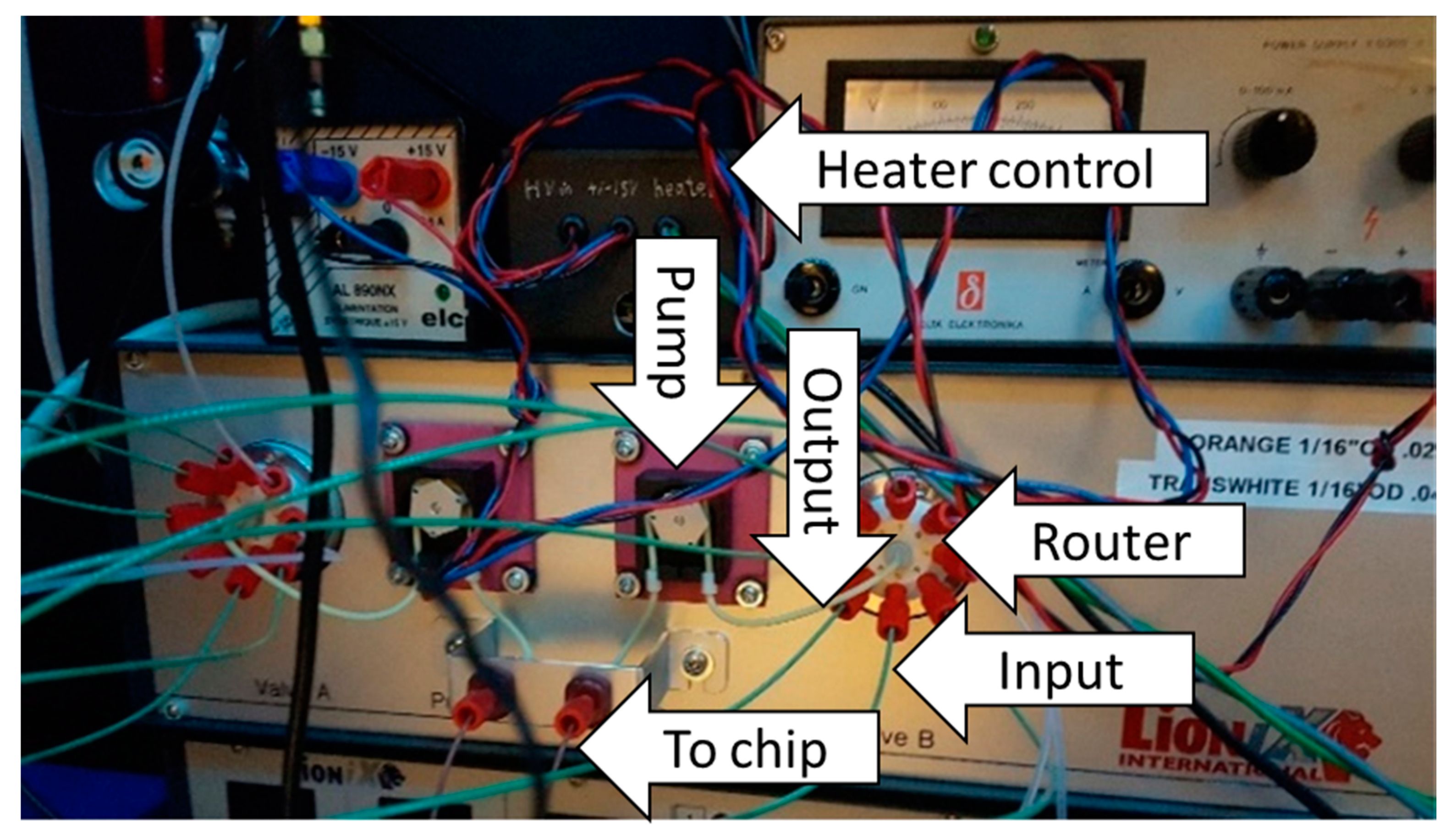
3.1.1. Chip Testing Hardware

In order to test the optofluidic chips, the light from an SLD was butt coupled to a PM input fiber of a fiber array (FA). A fiber tower was built to facilitate the experiments. It consisted of a breadboard and 12 narrow key–slot mating sleeves. The chips were mounted on a bisected chip holder and placed on a translation stage with six degrees of freedom (Thorlabs Nanomax Max607/M, Newton, NJ, USA). The fiber array was placed upon a second translation stage (Thorlabs Nanomax 300, Newton, NJ, USA). The facet of the fiber array was butt coupled to the chips without the aid of an index matching gel. Two PM fibers (FC/APC—SMA) were coupled to the output fibers and connected to the recording devices. The output of a power meter (S150C, Thorlabs, Germany) was used to optimize the alignment of the FA and the chip. The SLD (BLMS-mini-521-HP, SuperlumTM, Carrigtwohill, Co. Cork, Ireland) with an integrated isolator (standard IO-J-980) provided polarized light with a 92.2 nm bandwidth at a central wavelength of 994.2 nm. A 7.8 mW output power, a spectral ripple of 1.6%, and a power drift of <0.3%/4 h were specified by the manufacturer.
Moreover, 50 mL stock solutions of Na2SO4 (0.0613, 0.125, 0.25, 0.5, and 1 M) were prepared to measure the optical response of the chips. The solutions were prepared using demineralized water and the salts (Sigma Aldrich, St. Louis, MO, USA) were weighed on a precision (±0.1 mg) balance (PIONEERTM, Ohaus, Florham Park, NJ, USA). All the solutions were flushed through 0.45 µm filters (Millipore Millex-LCR, VWR, Amsterdam, NL, The Netherlands) to prevent the clogging of the microfluidic channels. An autosampler (see Figure 8) built by LioniX was used to deliver both samples to and flush the microfluidic system with demineralized water. The device consisted of two peristaltic pumps (p625/900.133) with eight rotary valves (eight outlets and one inlet). The pumps could be controlled separately with an Arduino microprocessor using LabVIEW software. Standard tubes (PEEK and 020P Pharmed, VWR, Amsterdam, NL, The Netherlands) of 50 cm were used to transport the solutions from 50 mL bottles to the microfluidic sampling channels on the chips.
Two spectrometers (Ava Spec-ULS3648, Avantes BV, Apeldoorn, NL, The Netherlands) with a sensitivity of 160 counts∙mW−1∙ms−1 and an optical resolution of 0.6 nm were used to record the transmission through the chips with an MZI, the second MZI on-chip, and the interferometer.

3.1.2. Chip Validation Procedure

When measuring the optical absorbance of the test solutions with the chips, the recorded spectral counts were normalized and converted to the dB scale with a MATLAB script (R2017b, the MathWorks, Natick, MA, USA). Figure 9 shows the next steps in the data analysis.
First, the peaks and valleys (maxima and minima) of the fringes were determined. Then, the maxima and minima were interpolated. The fringe depth was then calculated by the subtraction of the fitted minima from the fitted maxima; and then finally, the mean and standard deviation of the fringe depth was calculated. A second MATLAB script was used to determine the fringe spacing. As expected, a nearly linear relation was observed between the fringe spacing and the wavelength. Therefore, the fringe spacing at 940 and 1040 nm could be fitted using a linear regression.
In Figure 10, the null depth (minimum amplitude level of the fringes) is plotted against the calculated geometric path length difference. Here, the error bar of the null depths represents the standard deviation of the 200 spectra, whereas the error bar of the geometric path lengths denotes the differences between the calculated geometric path length from the fringe spacing at 940 and 1040 nm.
The influence of ionic solutes on the transmission spectrum of water was determined by recording a data set for two chips to avoid chip-specific problems. To collect these data sets, the following procedure was used: first, 200 baselines were recorded after both fluidic channels were flushed with demineralized water. Then, the sample channel was flushed by the sample of the solution to be measured (five times 1 mL). Subsequently, 200 additional spectra were collected. This step was repeated for each sample until the highest concentration (1 M) was reached. Finally, the sample channel was flushed (five times 1 mL) with distilled water and 200 spectra were recorded. The solutions were automatically and sequentially flushed through channels.

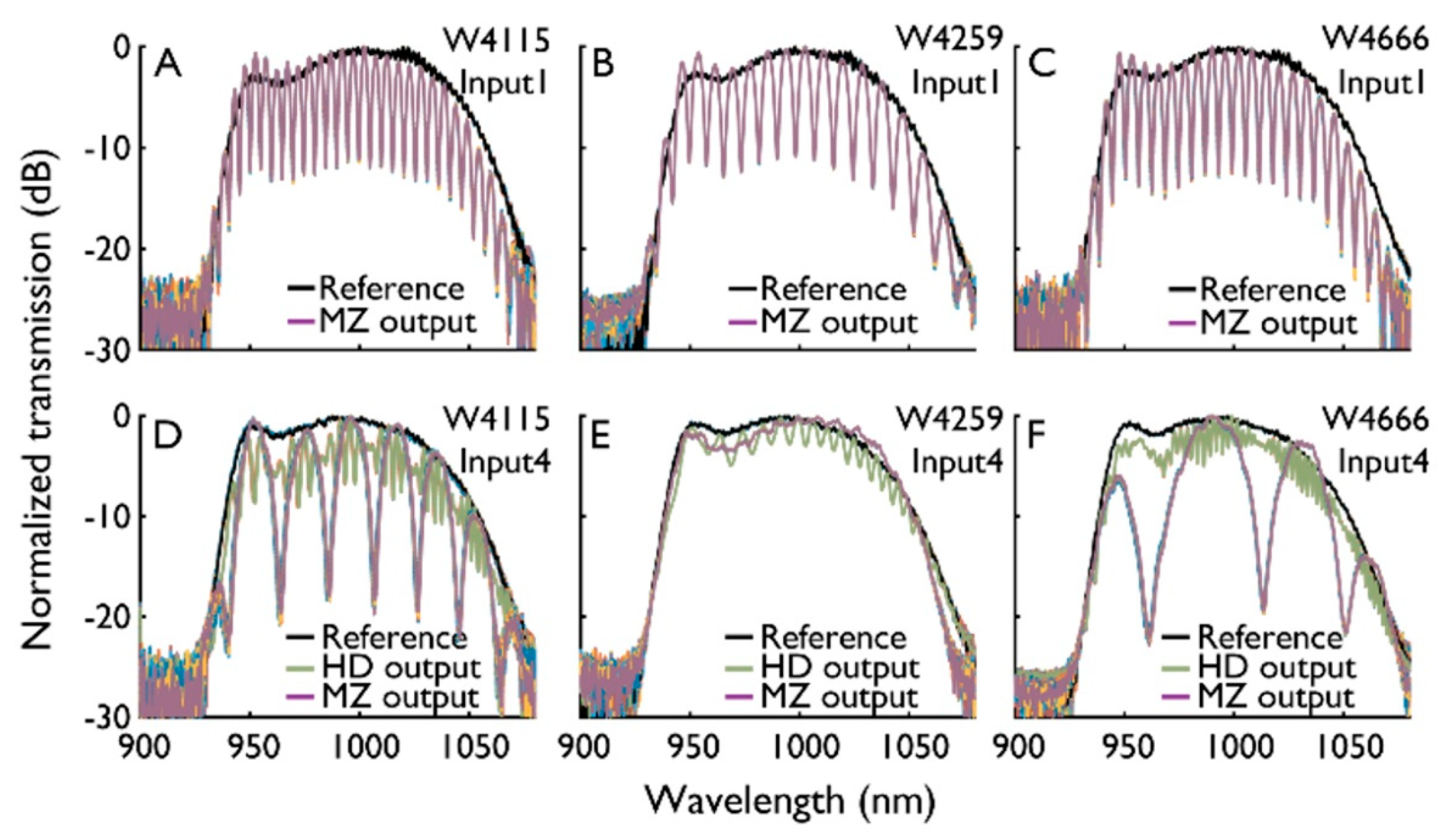
4. Experimental Results and Discussion

Figure 11 shows the normalized output (signal) of the MZI on the chip and interferometer. The signals from the MZIs and interferometers showed rather large variations in the fringe spacing for the same optical design between the different wafers. Whereas the actual path length is naturally the same for the same design, the optical path length may not be, since it depends also on the etching process, which has not been 100% reproducible. A small difference in the etch depth and/or width/thickness of the waveguide can thus change the optical cross-section, and the effective refractive index. These changes in the effective refractive index will consequently result in deviations from the designed spectral output: Since the sensing and reference arms are rather long (5 cm), a refractive index difference of 1 per mille will add 50 µm pathlength difference.
The small modulation (independent from ion concentration) on the input spectra likely originates from an optical cavity between the fiber array and the chip. The variations in fringe spacing are probably due to differences in the optical cross-section of the buried waveguides between the two arms of the MZI. The optical cross-section and fringe spacing at 940 and 1040 nm should result in the same calculated geometric path length differences. The fact that they do not points at the possibility that the cross-sections of the fabricated chips deviate from those in the simulations.
A direct correlation of the analyzed signal (null depth and fringe spacing, see Figure 10) to the four designed optical path differences proved to be more difficult than expected. Still, high-fringe depths were recorded (Figure 11A–C) close to what is theoretically possible with the 0.6 nm resolution of the spectrometers. In the homodyne design, the MZI output was successfully mixed with the local oscillator, as can be seen from the secondary modulation of fringes in Figure 11D–F. Additionally, the differences in the optical power between the output of the MZI (sensing path) and interferometer (sensing path + buried path) for the different chips indicates that the propagation losses (the sensing paths) varied from chip to chip, again probably due to the insufficient reproducibility of the etching process. This creates an uncertainty in the amount of homodyne amplification that requires additional calibration per chip.
However, a fringe modulation with only a single periodicity dependent on ionic concentration was indeed observed for the MZI output, verifying the intended single mode operation. The fringe spacing as well as the null depth as a function of the concentration of Na2SO4 is given in Figure 12.
It should be pointed out here that the measured null depths (Figure 12) differ from the calculated ones (Figure 3). Whereas it is difficult to pinpoint the exact reason for this mismatch, it could be due to small fabrication deviations between the waveguides of the MZI arm leading to a different absorption cross-section, and thus an increase in power imbalance. The change in the imaginary part of the refractive index cannot be easily recovered by the fitting of the spectral data without knowing the actual absorption cross-section of both MZI arms. Unfortunately, it is almost impossible to determine this parameter experimentally.

5. Conclusions

We have shown that with interferometric techniques, the qualitative and quantitative measurements of ions in aqueous solutions with an optofluidic chip are possible. This feature is achieved by comparing the complex refractive indices of the sample and reference as well as differential absorption signals. A simulation also showed that the differentiation between and the measurement of four different electrolytes is possible.
The initial experimental results revealed that the fabricated chips operated in the desired single mode. High contrast in the visibility was observed with a highest null depth of (29 ± 2) dB. The experiments with Na2SO4 showed the chips to be sensitive to changes in the real and imaginary part of the refractive index caused by the ionic content in water. Differences between the theoretical and measured null depths were probably due to fabrication deviations on the Si3N4 core.
At the present stage, the optofluidic chips could make use of the change in the real and imaginary part of the refractive index to quantify the ionic content in the water. In order to also experimentally identify different ions, a refined chip production and more research are necessary.

Author Contributions

Conceptualization, H.L.O. and G.W.S.; methodology, H.L.O. and G.W.S.; software, G.W.S.; writing—original draft preparation, G.W.S.; investigation, G.W.S.; writing—review and editing, E.C.F., A.D.W., H.L.O.; supervision, H.L.O., A.D.W., E.C.F.; project administration, E.C.F., H.L.O., A.D.W. All authors have read and agreed to the published version of the manuscript.

Funding

Wetsus is cofunded by the Dutch Ministry of Economic Affairs and Ministry of Infrastructure and Environment, the European Union Regional Development Fund, the Province of Fryslân, and the Northern Netherlands Provinces.

Acknowledgments

This work was performed at Wetsus, European Centre of Excellence for Sustainable Water Technology (www.wetsus.nl). Wetsus is funded by the Dutch Ministry of Economic affairs, the European Union Regional Development Fund, the Province of Fryslân, the City of Leeuwarden and the EZ/Kompas program of the “Samenwerkingsverband Noord-Nederland”. The authors like to thank the participants of the research theme “Sensoring” for the fruitful discussions and their financial support. We acknowledge Martin Visser for his contribution in the experimental work.

Conflicts of Interest

The authors declare no conflict of interest.

References

  1. Plant, J.A.; Voulvoulis, N.; Ragnarsdottir, K.V. (Eds.) Pollutants, Human Health and the Environment: A Risk Based Approach; John Wiley & Sons: Hoboken, NJ, USA, 2012. [Google Scholar]
  2. Argos, M.; Kalra, T.; Rathouz, P.J.; Chen, Y.; Pierce, B.; Parvez, F.; Sarwar, G. Arsenic exposure from drinking water, and all-cause and chronic-disease mortalities in Bangladesh (HEALS): A prospective cohort study. Lancet 2010, 376, 252–258. [Google Scholar] [CrossRef] [Green Version]
  3. Knobeloch, L.; Salna, B.; Hogan, A.; Postle, J.; Anderson, H. Blue babies and nitrate-contaminated well water. Environ. Health Perspect. 2000, 108, 675. [Google Scholar] [CrossRef] [PubMed]
  4. Kumar, M.; Puri, A. A review of permissible limits of drinking water. Indian J. Occup. Environ. Med. 2012, 16, 40. [Google Scholar] [PubMed] [Green Version]
  5. World Health Organization, WHO/UNICEF Joint Water Supply, & Sanitation Monitoring Programme. Progress on Sanitation and Drinking Water: 2015 Update and MDG Assessment; World Health Organization: Geneva, Switzerland, 2015. [Google Scholar]
  6. Alblasserdamsnieuws (Online-Newspaper), Ook Genx Aangetroffen in Alblasserdams Leidingwater. Available online: http://www.alblasserdamsnieuws.nl/wordpress/2017/04/21/ook-genx-aangetroffen-in-alblasserdams-leidingwater-d66-wil-landelijke-aandacht (accessed on 12 July 2017).
  7. AD (Online-Newspaper), Bron van Drinkwater in Deel Randstad Vervuild Met Gif. Available online: http://www.ad.nl/nieuws/bron-van-drinkwater-in-deel-randstad-vervuild-met-gif~a3350191/ (accessed on 12 July 2017).
  8. Huisman, J. Ziektegevallen na Verontreiniging van Drinkwater Met Fenol; een Engelse Ervaring. H twee O Tijdschr. Watervoorzien. Afvalw. 1985, 18, 433. [Google Scholar]
  9. Coussens, C. (Ed.) Global Environmental Health: Research Gaps and Barriers for Providing Sustainable Water, Sanitation, and Hygiene Services: Workshop Summary; National Academies Press: Washington, DC, USA, 2009. [Google Scholar]
  10. Reynolds, K.A.; Mena, K.D.; Gerba, C.P. Risk of waterborne illness via drinking water in the United States. In Reviews of Environmental Contamination and Toxicology; Springer New York: New York, NY, USA, 2008; pp. 117–158. [Google Scholar]
  11. Parnell, G.S.; Smith, C.M.; Moxley, F.I. Intelligent adversary risk analysis: A bioterrorism risk management model. Risk Anal. 2010, 30, 32–48. [Google Scholar] [CrossRef] [PubMed]
  12. Clarke, S.C. Bacteria as potential tools in bioterrorism, with an emphasis on bacterial toxins. Br. J. Biomed. Sci. 2005, 62, 40–46. [Google Scholar] [CrossRef] [PubMed]
  13. Gleick, P.H. Water and terrorism. Water Policy 2006, 8, 481–503. [Google Scholar] [CrossRef] [Green Version]
  14. Pujol, L.; Evrard, D.; Groenen-Serrano, K.; Freyssinier, M.; Ruffien-Cizsak, A.; Gros, P. Electrochemical sensors and devices for heavy metals assay in water: The French groups’ contribution. Front. Chem. 2014, 2, 19. [Google Scholar] [CrossRef] [PubMed] [Green Version]
  15. Bodini, M.E.; Sawyer, D.T. Voltammetric determination of nitrate ion at parts-per-billion levels. Anal. Chem. 1977, 49, 485–489. [Google Scholar] [CrossRef] [PubMed]
  16. Bansod, B.; Kumar, T.; Thakur, R.; Rana, S.; Singh, I. A review on various electrochemical techniques for heavy metal ions detection with different sensing platforms. Biosens. Bioelectron. 2017, 94, 443–455. [Google Scholar] [CrossRef] [PubMed]
  17. Murrihy, J.P.; Breadmore, M.C.; Tan, A.; McEnery, M.; Alderman, J.; O’Mathuna, C.; Glennon, J.D. Ion chromatography on-chip. J. Chromatogr. A 2001, 924, 233–238. [Google Scholar] [CrossRef] [Green Version]
  18. Dai, Y.; Liu, C.C. A simple, cost-effective sensor for detecting lead ions in water using under-potential deposited bismuth sub-layer with differential pulse voltammetry (DPV). Sensors 2017, 17, 950. [Google Scholar]
  19. Chaplin. Available online: http://www1.lsbu.ac.uk/water/water_vibrational_spectrum.html (accessed on 21 June 2018).
  20. Steen, G.W.; Fuchs, E.C.; Wexler, A.D.; Offerhaus, H.L. Design Considerations to Realize Differential Absorption-Based Optofluidic Sensors for Determination of Ionic Content in Water. IEEE Sens. J. 2018, 18, 6051–6058. [Google Scholar] [CrossRef] [Green Version]
  21. Zhuang, L.; Marpaung, D.A.I.; Burla, M.; Beeker, W.; Beeker, W.P.; Leinse, A.; Roeloffzen, C.G.H. Low-loss, high-index-contrast Si3N4SiO2 optical waveguides for optical delay lines in microwave photonics signal processing. Opt. Express 2011, 19, 23162–23170. [Google Scholar] [CrossRef] [PubMed] [Green Version]
  22. Steen, G.W.; Fuchs, E.C.; Wexler, A.D.; Offerhaus, H.L. Identification and quantification of 16 inorganic ions in water by Gaussian curve fitting of near-infrared difference absorbance spectra. Appl. Opt. 2015, 54, 5937–5942. [Google Scholar] [CrossRef] [PubMed] [Green Version]
  23. Roeloffzen, C.G.H.; Hoekman, M.; Klein, E.J.; Wevers, L.S.; Timens, R.B.; Marchenko, D.; Geskus, D.; Dekker, R.; Alippi, A.; Grootjans, R.; et al. Low-Loss Si3N4 TriPleX Optical Waveguides: Technology and Applications Overview. IEEE J. Sel. Top. Quant. Electr. 2018, 24, 4400321. [Google Scholar] [CrossRef] [Green Version]
  24. Steen, G.W.; Wexler, A.D.; Fuchs, E.C.; Bakker, H.A.; Nguyen, P.D.; Offerhaus, H.L. Role of temperature in de-mixing absorbance spectra composed of compound electrolyte solutions. Appl. Opt. 2018, 57, 7871–7877. [Google Scholar] [CrossRef] [PubMed]
  25. Pissadakis, S.; Selleri, S. (Eds.) Optofluidics, Sensors and Actuators in Microstructured Optical Fibers; Woodhead Publishing: Sawston, UK, 2015. [Google Scholar]
  26. Fainman, Y.; Lee, L.; Psaltis, D.; Yang, C. Optofluidics: Fundamentals, Devices, and Applications; McGraw-Hill, Inc.: New York, NY, USA, 2009. [Google Scholar]
  27. Hlubina, P. Dispersive white-light spectral two-beam interference under general measurement conditions. Opt. Int. J. Light Electron Opt. 2003, 114, 185–190. [Google Scholar] [CrossRef]
  28. Eberhart, R.; Kennedy, J. A new optimizer using particle swarm theory. In Micro Machine and Human Science, 1995. MHS’95, Proceedings of the Sixth International Symposium on Micro Machine and Human Science, Nagoya, Japan, 4–6 October 1995; IEEE: Piscataway Township, NJ, USA, 1995; pp. 39–43. [Google Scholar]
  29. Clerc, M.; Kennedy, J. The particle swarm-explosion, stability, and convergence in a multidimensional complex space. IEEE Trans. Evol. Comput. 2002, 6, 58–73. [Google Scholar] [CrossRef] [Green Version]
Figure 1. (A) Schematic representation of the optical configuration. The purple line represents the input which is split into a top (red) pathway that indicates the sample arm and a blue pathway that represents the reference arm. The two are recombined and then split again, so that half of one of the signals can be measured directly and the other half can be used for further interference with the local oscillator (indicated in light green). The black line serves as a reference of the input spectrum. (B) The mask design. The light red, black, and dark green lines represent the buried waveguides, sensing waveguide, and the gold deposit, respectively. The light blue areas are the fluidic channels (sample on top, reference below). The pathway of the light is marked in dark red, blue and violet for the sample arm, reference arm and their combination, respectively. The red rectangular object in the left lower corner is a delay spiral for the local oscillator. The path going to (and back from the) spiral is marked in bright green. At the rectangular light purple areas in the channels, the top cladding was etched away to allow interaction between the light and the fluid. The waveguides positioned at the edge of the chip (the left side) are tapered to allow butt coupling with the fibers. The violet arrows show the input and output, and the violet/green dashed line is the output including the interferometric amplification.
Optics 01 00014 g001
Figure 2. The spectral transmission determined for a geometric path different from (A) 0.30 to 0.34 µm, (B) 59.5 µm, (C) 150 µm, and (D) 300 µm. The optical path can be (limited) dynamically controlled by applying current to the heaters. Subfigure (A) shows the transmission response for a small change in the geometric path length: I = 0.30 µm, II = 0.31 µm, III = 0.32 µm, IV = 0.33 µm, and V = 0.34 µm.
Optics 01 00014 g002
Figure 3. The effect of the path differences and the resolution of the recording device on the null depth. (A) Line plots marked with roman letters I–IX for the resolution of 0.05, 0.1, 0.2, 0.3, 0.4, 0.5, 0.6, 0.7, 0.8, 0.9, and 1.0 nm. (B) Line plots marked with the roman letters I–XVII for the optical path difference from 50 to 450 µm in steps of 25 µm.
Optics 01 00014 g003
Figure 4. Simulated fringe spacing around 940 and 1040 nm (solid and dashed blue line, respectively) and the number of fringes (red solid line) for a 100 nm broadband light centered at 990 nm, guided by a 1.6 µm by 92 nm Si3N4 core surrounded by SiO2, for the different geometric path differences of the integrated Mach–Zehnder interferometer.
Optics 01 00014 g004
Figure 5. Linear regression fits of the Gaussian curves representing Pb(NO3)2. (A) The four Gaussian amplitudes as a function of electrolyte concentration and (D) the residuals of the fits. Likewise the (B) position, and (C) the width of the four Gaussian curves against electrolyte concentration and (E,F) their respective residuals.
Optics 01 00014 g005
Figure 6. Calculated spectral visibility and null depth against the concentration of Na2SO4.
Optics 01 00014 g006
Figure 7. The fit of a mixture of four electrolytes. (A) The determined spectral transmission and its fit, (B) the residual of the transmission data, (C) the expected visibility data and its fit, (D) the residuals of the visibility fit, and (E) the performance of the fit.
Optics 01 00014 g007
Figure 8. Photograph of the autosampler built by LioniX to flush the microfluidic channels with the solutions. On top of the autosampler, the heater control units are located.
Optics 01 00014 g008
Figure 9. A visual example of the data-processing algorithm. The peak and valleys of the fringes are located in the averaged data. From the values, the average fringe depth over a spectral bandwidth of 100 nm is determined.
Optics 01 00014 g009
Figure 10. The performance of the Mach–Zehnder interferometers (MZI). The solid black line is the expected null depth from a recording device with a resolution of 0.6 nm. The vertical colored red, blue, orange, and green line indicates the designed MZI with a geometric path length difference of 0.3, 59.5, 150, and 300 µm, respectively. The data points from the different designs are outlined with a colored circle.
Optics 01 00014 g010
Figure 11. Input (black), MZI output (purple) and homodyne output (green) against the wavelength for the three wafers (columns) and two pathlength differences (rows). The top row (AC), represents an MZI with a 50 µm pathlength difference which corresponds to 10 fringes over the spectrum. (DF) represents an MZI designed to have zero pathlength difference. Half of the output of the MZI is recorded directly (MZI, purple), and the other half is recombined with the local oscillator to realize the homodyne (HD, green) output.
Optics 01 00014 g011
Figure 12. The shift of the fringes and change in null depth for the different concentrations of Na2SO4. The analyzed data of two on-chip MZI were intended to have 10 spectral fringes (A,B).
Optics 01 00014 g012

