Simulation of Oil Well Drilling System Using Distributed–Lumped Modelling Technique

1
Department of Aeronautical and Automotive Engineering, Loughborough University Loughborough, Leicestershire LE11 3TU, UK
2
Department of Mechanical Engineering Technology, Yanbu Industrial College, Yanbu 30436, Saudi Arabia
*
Author to whom correspondence should be addressed.
Modelling 2020, 1(2), 175-197; https://0-doi-org.brum.beds.ac.uk/10.3390/modelling1020011
Submission received: 11 August 2020
/
Revised: 29 October 2020
/
Accepted: 4 November 2020
/
Published: 12 November 2020
Abstract
:The strengths and torque of well-boiling hydrocarbons are of utmost significance. Boiling a well is one of the most critical steps in the discovery and production of oil and gas. The well’s boiling process is expensive because the drilling depth can be as much as 7000 meters. Any delay (breakdown time) in boiling costs a lot of money for hydrocarbon firms. Various boiler parameters are continuously tracked and regulated to avoid drilling delays. This paper focuses on the vibrations occurring at the bottom hole assembly (BHA) stick-slip. Two modelling methods, the lumped parameter model and the combination of the distributed–lumped (D–L) parameter model, were used and compared to the actual measurement performance. The D–L model was found to be more precise, particularly for long strings. Using the simulations, the most comprehensive modelling methodology is introduced.
1. Introduction
Drilling processes in the petroleum industry are extremely costly. The drill bit penetrates via a mechanism affected by the drilling rocks. The axial vibrations, lateral vibrations (the longitudinal bit bounce phenomenon known as the whirl motion), and torsional vibrations are classified into three main categories during the drilling process.
Axial vibrations: Axial vibrations are caused by the irregular movement of the drill string on the longitudinal axis, thus leading to the bit-bounce [1,2]. It may cause damage to the extreme shape of the bit, bearing, and bottom hole assembly (BHA) [3]. The bit bounce causes the bit to lose the drilling rock touch, which delays the penetration.
Lateral vibrations: Lateral vibrations consist of some of the most destructive string oscillations [4,5]. During rotation, the pipe’s eccentricity sometimes results in centripetal forces, resulting in what is called a drill string whirl. This whirl can also be caused by the plot entering the borehole walls under lateral vibrations, which may result in the eccentric hole, wall damage, damage to the BHA, and an incorrect drilling direction [6,7]. Additionally damaged is the drilling pull. All this contributes to the postponement of the entire cycle. The connection between the BHA and the contact points of the drill cord cause the unit to turn backward or forward in some cases. A backwards whirl is the most extreme vibration that causes fatigue at the moment of large-frequency bending. Unbalancing in an assembly causes a centrifugal bowing of the drill string, which may lead to a front whirl and partial wear on one side [5,8].
Torsional vibrations: Torsional vibration, called stick-slip, is typically responsible for a nonlinear interaction between the bits and the rock or between the drill string and the borehole wall. Stick-slip vibration typically occurs during drilling and is an extreme type of the torsional oscillation of the drill string in which the bit for a fraction of the drilling time becomes stationary. Torsional vibrations are more suitable than forced self-exiting (through axial vibrations) [9,10].
The non-linear relationship between the torque and angular velocity on the bit is responsible for stick-slip motion. Even when the engine steadily turns the bit [11,12], the drilling and BHA over the engine push around the stick/slip. Torsional vibrations induce drill brace fatigue, slow the process of boiling, and damage bits, drilling pipes, and the BHA.
In different studies that have been focused on modelling drilling behaviour, the three classes of vibrations have been separate or combined [1,2,3,4,5,6,7,8,9,10,11,12]. The focus of this article is on the BHA’s torsional vibration. The related phenomenon is that the top portion of the drill line rotates at a constant rotational speed, while the bit of the rotational speed varies from zero to up to six times the surface rotational speed. This paper introduces a model of a lumped parameter and a hybrid model consisting of the drilling system’s distributed–lumped parameter model.
The string is considered as a two-degree free torsional pendulum in the lumped model and represents normal differential equations, which implies that there is one independent variable (i.e., time) in device analysis. In modelling systems, spatial variations are not important.
A mixture of ordinary and partial differential equations [13,14,15] describes the distributed–lumped (D–L) parameter model, as opposed to the lumped model. The normal differential equations describe the behaviour of the lumped model (drive systems and the BHA with the friction of the bit–rock interaction) and partial differential equations, the behaviour of the distributed model (drill pipes).
The D–L parameter model is a hybrid modelling technique defined by a combination of ordinary and partial difference equations. The lump parameter and distributed parameter models of an interconnected model with partial differential equations are represented by normal differential equations. D–L modelling is based on the approach of the transmission line matrix (TLM). This is a numbering strategy that was originally created to enable engineers to explain electromagnetic problems in the field of electrical and electronic engineering [14,15].
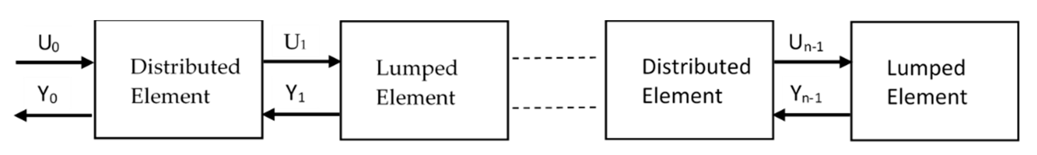
The hybrid model of intertwined lumped and distributed dynamic components, proposed by Robert Whalley in [13], is represented in Figure 1. Distributed elements are separated by lumped elements, where each item’s output represents the input of the element. For that modelling process, one basic rule is that the model should end up in a lumped product.
2. Model Description
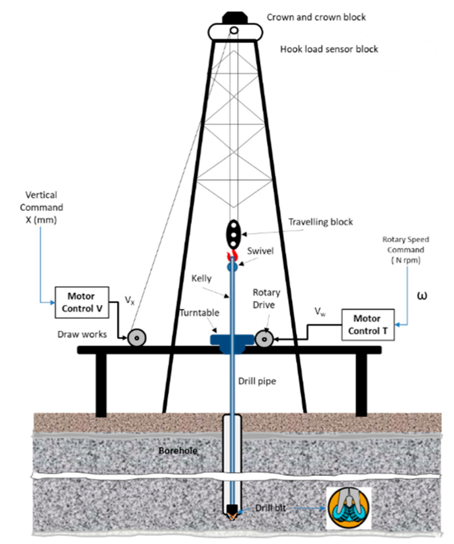
A basic rotary drilling method was taken into account for this analysis; see Figure 2. This type of drilling system was used because the most common drilling system is now used to reach the reservoirs of fossil fuel below the surface of the earth. By spinning a drill bit, the rotating drilling mechanism produces a drill hole. Normally, an electric motor mounted on the surface supplies the energy for rotation.
The electric motor drives the rotary table via a mechanical gearbox. A rotating table in the form of large disk has inertia that works as the kinetic storage of energy. A high-grade steel pipeline named Kelly provides the kinetic energy for the string via the revolving surface. The Kelly pipeline has a hexagonal external shape at the top of the drill line. It passes through the rotary table and connects to a swivel.
A dynamometer is used to pump a substance called mud down to the base of the well to help cut the process. The mud aids the cutting through the drilling bit by jetting, refreshes and lubricates the bit, and moves the cutting rocks from the bottom of the well to the surface, where mud is examined to assess where the drill bit has penetrated the earth layer and whether oil or gas traces remain.
A drill string mainly consists of drill pipes that are 9–10 m long and 0.73–0.14 m high and that are connected to the BHA at the bottom of the drill pipes [16,17,18]. The BHA consists of a heavyweight drill pipe, drill collars, and stabilizers, and it is at the bottom the drill bit.
A heavyweight drill pipe is used as a transition section between the drill pipe and the drill collar to reduce the generated stress between them. The drill collars in the BHA are kept in position by several stabilizers, which are short sections with nearly the same diameter as the bit [19,20].
The BHA consists of the heaviest section of the drill string and supplies the required weight on bit (WOB). The WOB, the rotary torque, and the hook load are the key operator parameters for the drilling operation. The breakdown time of the drilling process can be significantly reduced by controlling these parameters [19].
3. Mathematical Models
The mathematical modelling of physical systems helps to predict and then optimize system performance and behaviour under varying conditions. Two models of the presented drilling system were developed for this study—the lumped model and the distributed–lumped model (hybrid).
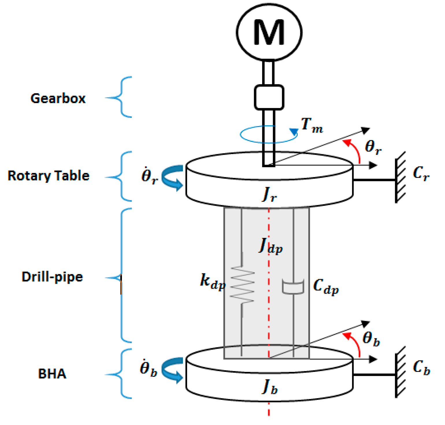
The torsional behaviour of the drill string in the lumped model has been described by a simple torsional pendulum driven by an electric DC motor. The drill pipes are represented as a linear spring of torsional stiffness and torsional damping . The drill pipes at the top side are connected to the inertia of the drive system (), and the drill pipes at the bottom side are connected to the inertia of the BHA (), which is considered the sum of the BHA inertia plus the of the drill pipes’ inertia. The bit–rock interaction was modelled by a dry friction model that was presented in [21,22].
On the other hand, for D–L modelling, the drill string of the drilling system is considered to be a shaft in torsion of length and diameter with shear modulus that has been described as a distributed parameter element. In this case, the inertia and stiffness of the shaft are a continuous function of its length. The scheme of the software drilling system used for lumped modelling is shown in Figure 3.
Due to the system design and the drilling process, it is believed that the drill string and the borehole are considered to be both vertical and straight, the drill bit does not exhibit lateral motion during the drilling process, the angular velocity of the high drive system is greater than 0, the drilling mud is simplified by a viscous-type friction element at the bit, and the drilling mud fluid orbital motion is considered to be laminar (no turbulences).
4. Lumped Model
The lumped model is a mathematical modelling technique concentrated on the pointwise features of a system. It is based on the use of ordinary differential equations (ODE) and applied to model systems in which spatial variation is not important.
The lumped modelling technique is considered to be a simpler modelling method compared to distributed modelling. The main feature of lumped models is that the signal is assumed to be transmitted from the input to the output of the element without delaying or distorting the next element in the system, but it does not consider the distance between components. These are the main differences between lumped and distributed modelling.
For this study, the drill string was viewed by the electric motor as a torsional pendulum that has two degrees of freedom. The drilling method was divided into three components for mathematical modelling.
4.1. The Drive System
First, one must provide the required torque for the drilling process, which consists of three main components: the electrical DC motor, which is the prime mover of the system and provides the torque () for the drilling operation, and the gearbox with bevel gear, which transfers the torque to the last part of the drive system, which is the rotary table.
4.2. The Drill String
In many cases, the modelling of the drill string is considered to be a torsional model of a conventional vertical drill string with two degrees of freedom [15], as reported in [13]. The two-degrees-of-freedom torsional model is presented in Figure 3, where the first mass represents the rotary table inertia (), which is affected by the motor and gearbox at the side of the motor, and the second mass represents the BHA inertia . The two masses are connected by the torsional coefficients of stiffness ) and damping ). The drill pipe is dumped due to the drilling mud, the structural damping of drill pipe, and friction between the drill pipe and wellbore.
4.3. The Cutting Process
The cutting process is the process where the drill bit cuts the rock and penetrates the stone layers. Due to the interaction between the drill bit and the cutting rocks, friction torque is generated. During the cutting process, stick-slip vibrations occur.
A non-linear frictional torque combines the sloppy vibrations of the oil drill string with a reactive torque when the bit is connected to the rocks and the non-linear frictional forces along with the BHA. Most drilling processes are modelled as a decreasing and constantly differentiated function in the modelling of friction torque when the velocity of the BHA does not equal zero and is otherwise discontinues because of the presence of Coulomb friction. The governing equations of motion for the described rotating system are:
where and are the torque of the rotary table transferred to the drill string and the reactive torque on the bit (TOB), respectively. The rotary torque equals the gear ratio of the gearbox times the torque supplied by the motor . The reactive torque on bit represents the combined effects of viscous damping torque on the BHA and non-linear frictional forces, along with the BHA, and is calculated by , where and (as is described later on the frictional torque model). is the overall inertia of the drive system that can be calculated from , where is the inertia of the rotary table and is the electric motor’s inertia. , and are the angular acceleration, angular velocity, and angular displacement of the rotary table, respectively.
The rotary table rotates at a constant speed regardless of the applied load, while the drill collars behave as a rigid body with an equivalent moment of inertia , where , and are the angular acceleration, angular velocity, and angular displacement of the bit, respectively. The equivalent moment of inertia, as can be seen in the following equations, includes the drill collar inertia , the heavy weight drill pipe (HWDP) inertia Jhdp, and 1/3 of the drill pipe :
where and ρ are the shear modulus and density for steel of the drill pipes, respectively , , and are the lengths of the drill collar, drill pipes, and heavyweight drill pipe, respectively. As the drilling operation proceeds deeper into the earth, the drill string length increases.
When new drill pipes are added to the drill string, the BHA length remains the same. Since drill pipe length increases during the drilling operation but the BHA length remains the same, their dynamics should be studied separately. and are the outer and inner diameters of the drill collar, respectively; and are the outer and inner diameters of the heavyweight drill pipe, respectively; and and are the outer and inner diameters of the drill pipe, respectively. The coefficients , and are the overall viscous damping coefficients of the drive system, the drill string, the BHA, and that along the drill pipe due to mud drilling, respectively. The damping coefficient along the drill pipe and the torsional stiffness of the drill pipe () can be calculated using the following equations.
5. Frictional Torque on the Bit
The friction torque applied on the bit due to the bit–rock interaction can be described using a variation of the Stribeck friction together with the dry friction model. The dry friction model can be approximated by a combination of the switch model proposed in [22] and a variation of Karnopp’s friction model (dry friction model) in which a zero-velocity band is introduced [23]. The friction model was used in [24] and is defined by Equation (7).
where .
Teb defines the applied external torque. It must overcome the static friction torque in order to make the drill bit rotate. Since the friction on the bit is proportional to the weight on bit (), the friction coefficient () equals the radius () of the bit. The friction torque on the bit is defined by: ; the static friction torque on the bit is: ; the Coulomb friction torque is: ; and is the limit velocity interval that specifies a small enough neighborhood of .
The dry friction torque for varies between the static friction torque and the Coulomb friction torque (). is the velocity depending dry friction coefficient at the bit, where .
and are the static and Coulomb friction coefficients, respectively, associated with the inertia , with ; is a positive constant defining the decaying velocity of .
Many models can be used to model the friction torque on the bit; most of these models use a reduced and continuous speed when the speed is not equal to zero and because there is discontinuous Coulomb friction. Together with the Stribeck effect, a dry friction model is used to form the friction torque on a bit [22,25]. The resulting friction model is presented and compared with a classical dry friction model with an exponential decaying law at the sliding phase [22,26]. Figure 4 shows a block diagram that represents the lumped model of a drilling system.
5.1. Distributed Model of the Rotating Shaft
Distributed modelling is a mathematical modelling method used to model dynamic systems. The authors of [18] stated that all physical systems are distributed in space, so for the sake of modelling, a model should also be distributed in the space to represent a real system. Distributed parameter models are used if a special configuration is very important. Distributed parameter models are very general models that can be used to simulate reservoirs with few or many grid-blocks. They allow for spatial variations in rock properties and thermodynamic conditions. The size of the distributed model plays an important role in the provided results—a bigger distributed model may give rise to errors such inaccuracy and delays. However, this is dependent on the experience of the modeler.
Distributed modelling is derived from the transmission line modelling method (TLM). Transmission line modelling was developed by electrical engineers at the beginning of the 1970s. It was developed for the calculation of voltage and current into electrical circuits, as well as for the propagation of electromagnetic waves through a manner (conductor). Over the years, new versions of the TLM have been developed to improve the modelling of arbitrary inhomogeneous media [27]. The TLM can be used to model events other than electric ones, such as mechanical and thermal events. The TLM is based on an electrical circuit where electrical elements substitute other elements.
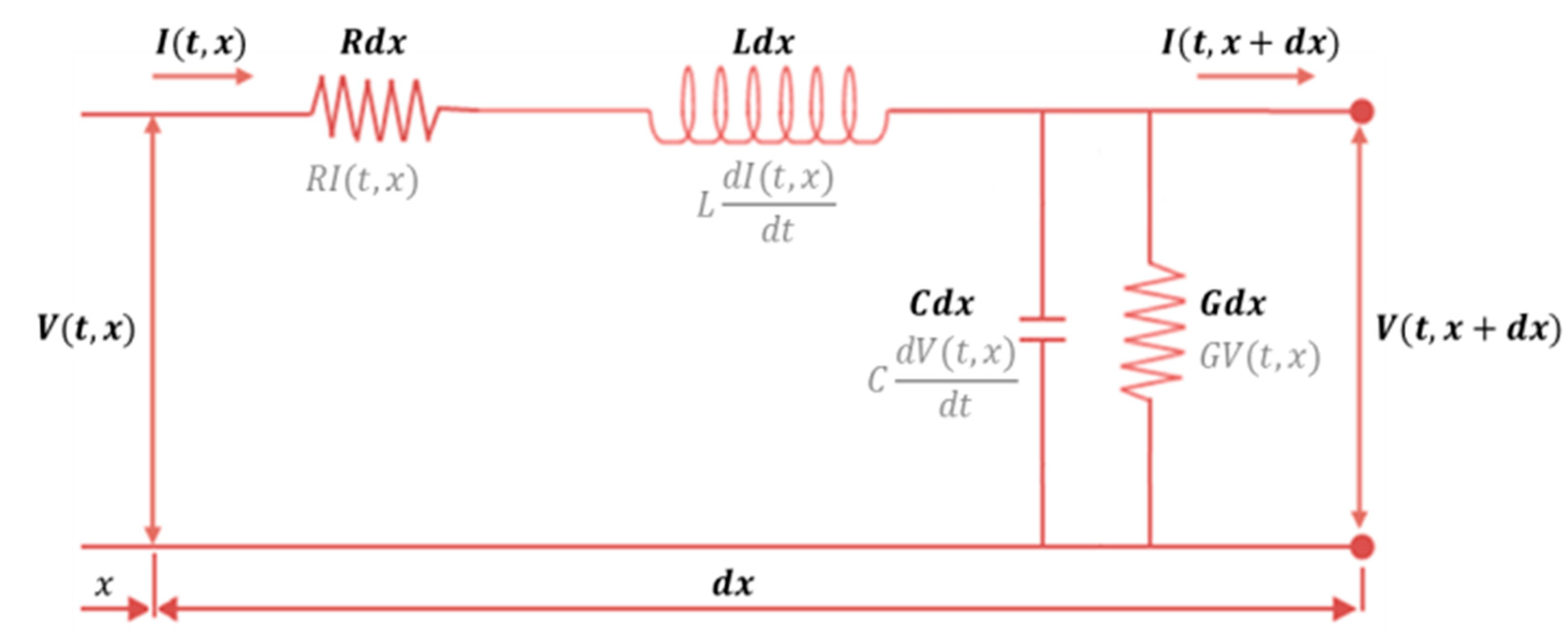
A transmission line is considered to be any medium that transfers electrical or mechanical power from one point to another, e.g., the electrical cables that transmit the electricity from electric stations to our homes. A transmission line comprises infinity infinitesimal elements. Each element comprises the primary constants of R (resistance), L (inductance), C (capacitance), and G (conductance). The primary constants for each infinitesimal element of a transmission line are multiplied by the length of the element . If the resistance (R) and conductance (G) are included in the analysis of a system, the transmission line is called a “lossy transmission line,” which represents losses in a system. On the other hand, if there are no losses, the model could be reduced to an ideal transmission line known as a “lossless transmission line” that only consists of inductance (L) and capacitance (C). Figure 5 shows the circuit representation of an infinitesimal element of a lossy transmission line.
Based on Figure 5, the presented elements have a voltage input at point , and, due to the voltage, an input current at point is generated. Therefore, the element has output voltage and output current . The voltage and the current in the presented circuit can be described using two equations that are based on Kirchhoff’s current and voltage law. The derived equations are known as telegrapher’s equations.
5.2. Torsional Shaft
The distributed torsional shaft comprises a well-known example of the transmission line system. The shaft comprises an infinite series of infinitesimal elements of length that transmit an applied torque from the input point to the output point. The electric circuit presented earlier has been used to model the interconnected infinitesimal elements of a torsional shaft. The shaft’s element has length and it is at distance from the input point of the shaft. Since the shaft is subjected to torque, each element has an input torque (torque at time at distance ) and an output torque (torque at time t and distance ) with corresponding input angular velocity and output angular velocity . The infinitesimal elements consist of a series inductance and a shunt capacitance , which for mechanical systems such as (in this case) a shaft are analogs to the inertia per unit length and the shaft’s compliance per unit length 1/GJ, respectively.
Based on the electrical circuit that was discussed earlier, the infinitesimal element has a series resistance series inductance , shut capacitance and shut conductance . The series resistance and the shut capacitance for the shaft analysis are usually neglected. This happens because the internal friction of the shaft and the external damping forces (due to the mud and the bearings) are neglected. The internal friction and external damping forces represent the losses of any system and, in this thesis, are considered in the lumped system model.
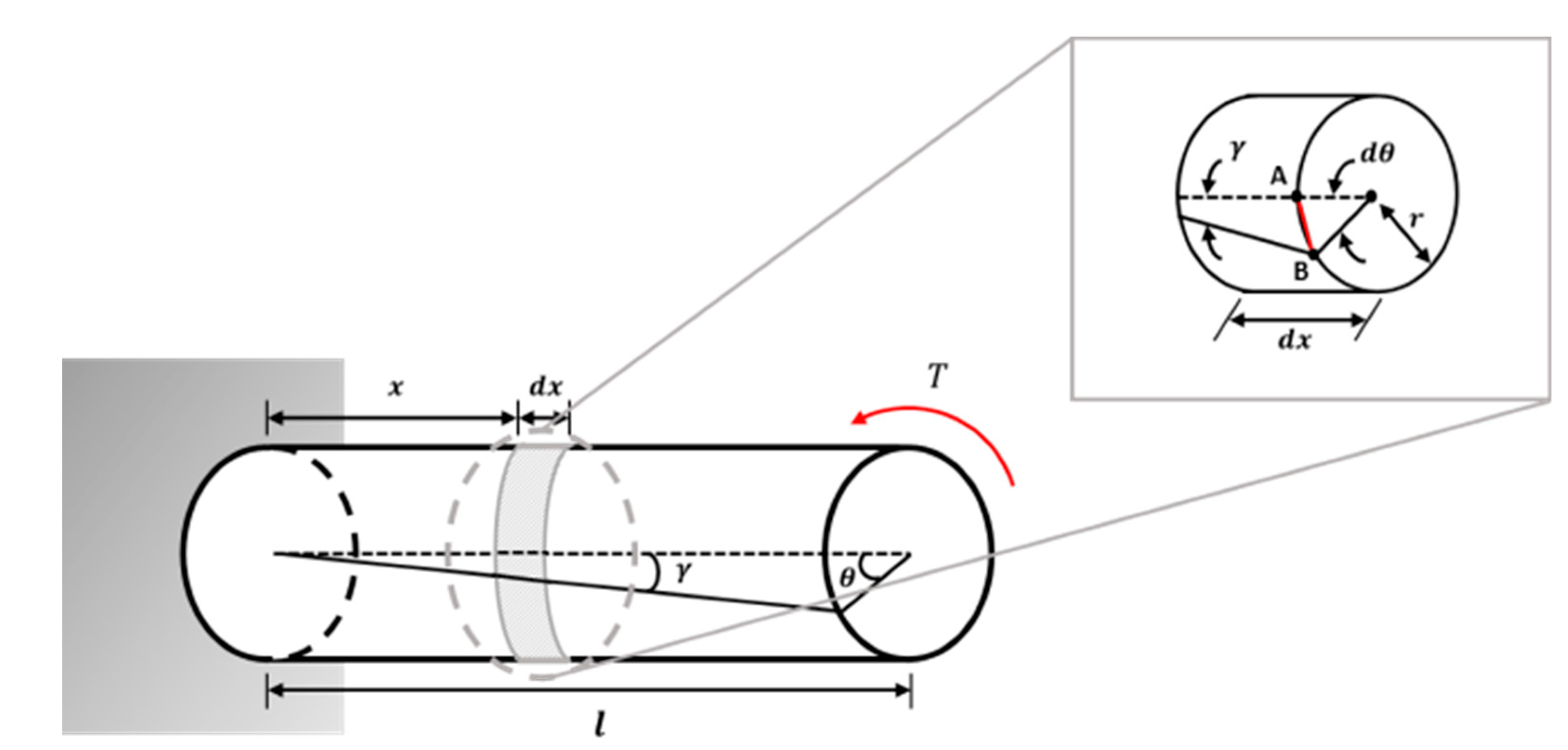
The drill string of a drilling system is considered to be a shaft in torsion with length and diameter . Shafts that are subjected to torque present the phenomenon of torsion. Torsion is a shaft’s (or any other object) twist due to an applied torque that leads to the rotation of one end relative to the other. The applied force leads to the generation of shear stress () on any cross-section of an object. As soon as the object starts to twist, the shear strain () occurs. Figure 6 shows a shaft of length and diameter that is fixed at one end and twisted at the other end, as well as a zoom view of a sliced section of the shaft after torque has acted upon it.
The relationship of the shear stress and shear strain can be expressed by applying Hooke’s law (Equation (8)):
If a small differential element of length is sliced from the bar, the two angles must be compatible at the outside edge (arc length A–B in red), where .
Using Hook’s Law, the change of angle can be found to be the shear strain produced by the shear stress. This assumption leads to the following relationship:
Substituting Equation (8) into Equation (9) and rearranging it in term of shear stress leads to:
where is the rate of the twist, which is related to the applied torque. To maintain rotational equilibrium, the sum of the moments contributed by the shear stress that acts on each differential area dA on the cross-section must balance the applied moment T:
Substituting Equation (10) into Equation (11) gives:
where and are considered constants, and is defined as the polar moment of inertia (J), which for a hollow shaft of internal diameter and outer diameter , is: .
Substituting the polar moment of inertia () into Equation (12) derives:
Rearranging Equation (13) in terms of the twisting angle leads to: . For a constant T, , and dA, , where .
The twisting angle can be substituted into Equation (10) to give shear stress: . From this relationship, one can assume that , and are constant along the shaft length. By substituting the two relations into the torsion formula (Equation (9)), the equation can be derived as: . Solving the above equation in terms of torque leads to:
where is the shear modulus of the pipe material and is the shaft polar moment of inertia .
The inertia torque acting on an element of length is , where is the density of the shaft and represents the mass polar moment of inertia per unit length. Using Newton’s second law () and transforming it for rotational motion, the equation of motion of the rotating shaft can be derived as: :
Taking the limit as approaches zero and dividing it by leads to:
Deriving the above equation with respect to leads to:
Considering that , Equations (16) and (17) can be expressed as:
where is the shaft inertia per unit length and 1/J = C is the compliance per unit length. The characteristic impedance and propagation of constant of the shaft are:
Considering the solution found in [28] for the lossless transmission line section, the general equation for the torsional system can be expressed as:
where the transform variable .
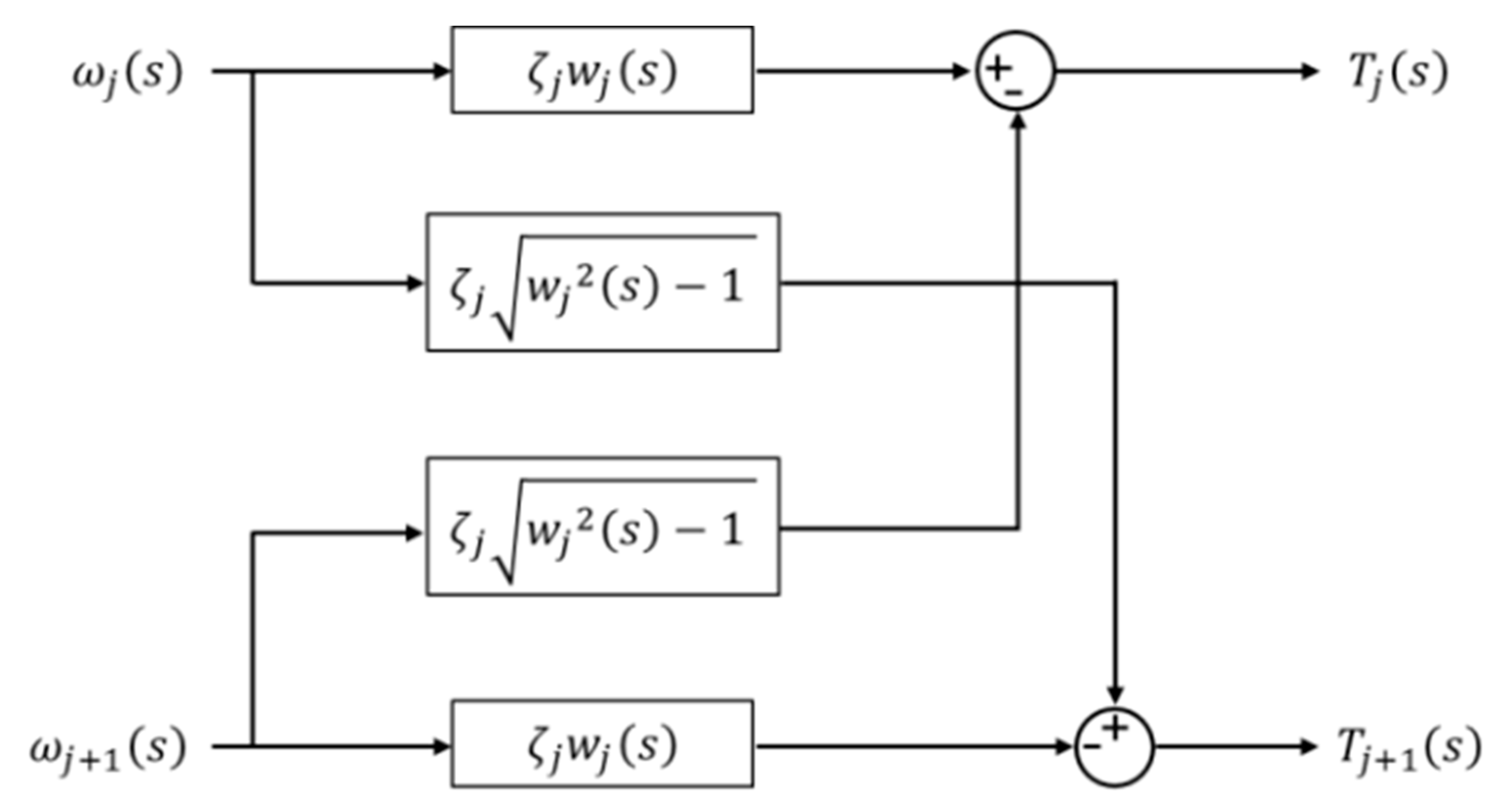
Figure 7 presents a block diagram of the mathematical model derived above (Equation (20)).
6. Hybrid Model of the Drilling System
Here, we present the distributed model of a drilling shaft that is interconnected with the two lumped models of the drive system and the BHA. In this case, the interconnected distributed–lumped parameter system is represented by a lumped–distributed–lumped (L–D–L) model. The distributed element from the D–L model is represented by matrix Equation (21), where the two lumped elements from the D–L model are represented by Equations (22) and (23).
where is the input torque to the drill pipes provided by the rotary table, is the input torque to the BHA applied by the drill pipes, is the angular velocity of the rotary table, is the angular velocity of the drill bit, and is the characteristic impedance of the distributed shaft, which is:
Additionally, is the transform variable of the distributed shaft, which can be derived as:
where is the shaft’s length and is the propagation constant that can be derived as:
At D–L modelling:
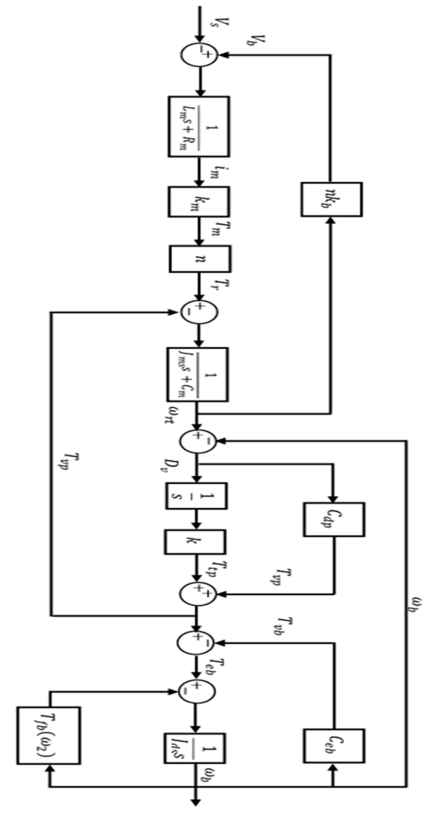
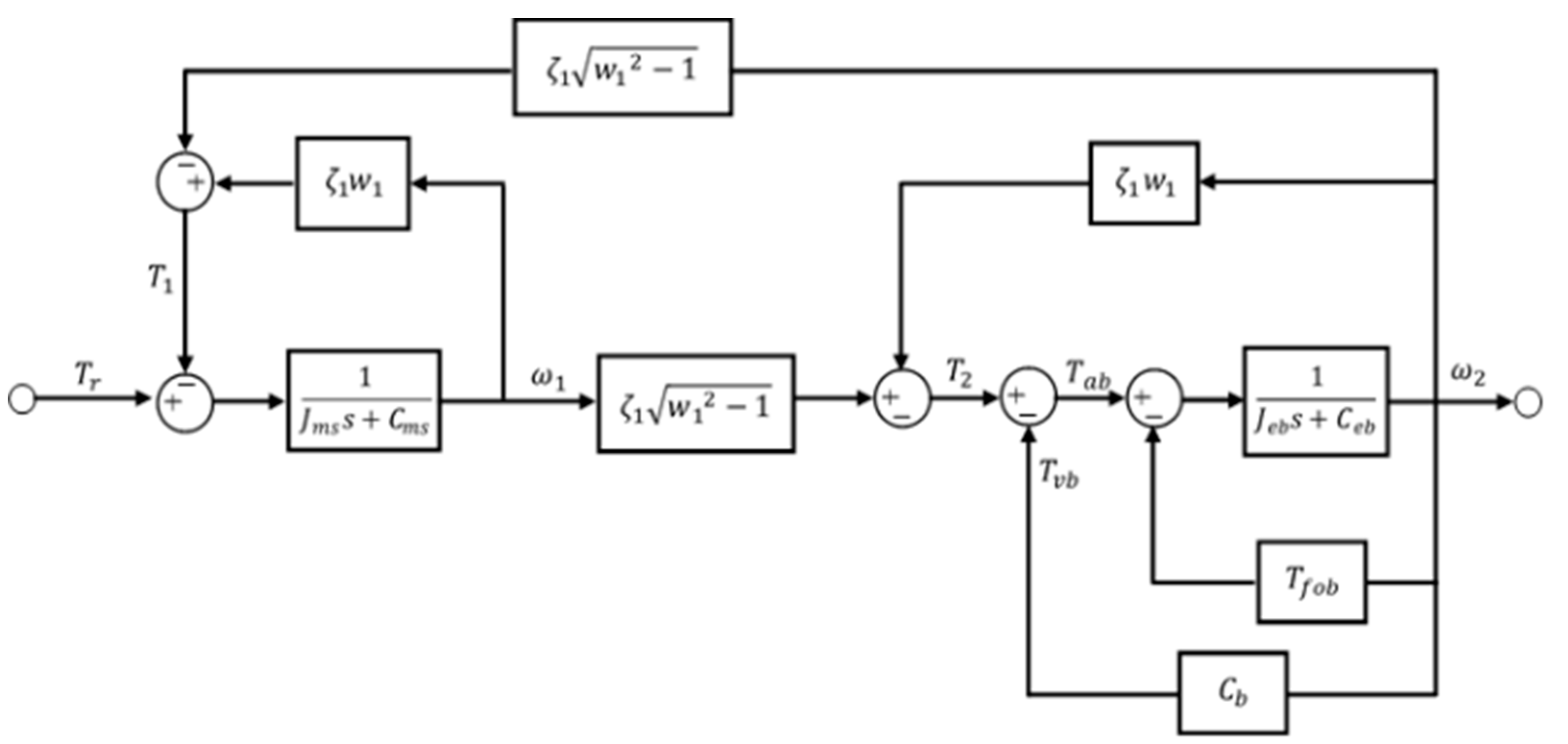
where Jms is the equivalent mass moment of the inertia of drive system, is the equivalent viscous damping of drive system, is the equivalent mass moment inertia of the BHA, is the equivalent viscous damping of the BHA, and is the friction torque on the bit due to the bit–rock interaction and is represented by the dry friction model. The applied torque on the bit () from the drill string in the D–L model is , where is the viscosity damping torque over the BHA. Figure 8 shows the derived D–L model of the presented drilling system.
7. Results and Analysis
7.1. Comparison of the Lumped Model and the D–L Model
After their development, the two models (the distributed–lumped model and the lumped model) had to be checked to see whether they provided the expected results, whether these results were accurate, and whether these models emulated the drilling process. To achieve that, the results were compared with real data that were found during the literature review [29].
Because MATLAB is a proprietary multi-paradigm programming language and numerical computing environment that allows for the plotting of functions and data, it was used to perform the required figures and comparisons of the models.
The comparison showed that the pipeline lengths were 2000, 5700, and 7500 m in three different scenarios. The two models were compared to find the best way to get stick-slip vibrations that were equal to those that occur during an actual drilling process. All models were tested for the different lengths and speeds of tubing. Both of them were tested with and without stick-slip vibrations.
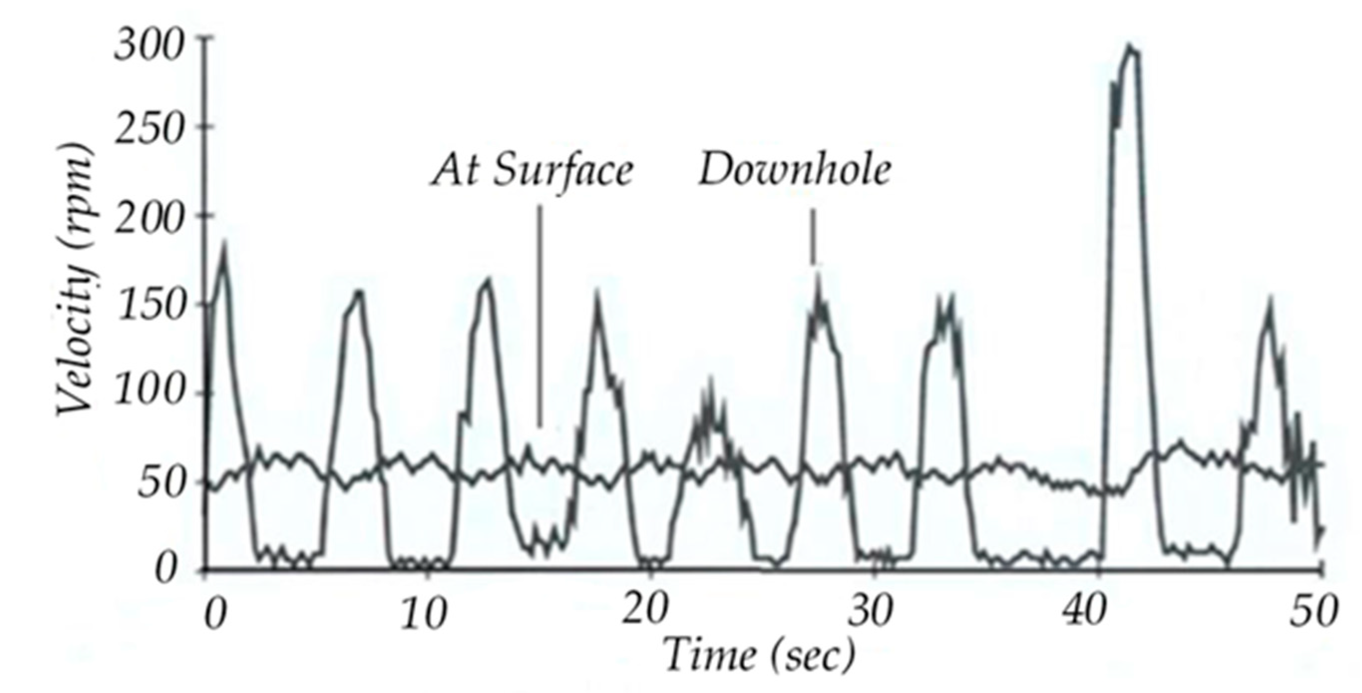
The variations between the two models were extracted at the end of the comparison. The critical speed was considered as the speed at which just stick-slip vibration occurred and above which stick-slip motion did not occur to show the differences between the two models. The comparison between the two models was focused on two main points—the first was related to the beginning of stick-slip motion and the end in both models when the angular velocity of the drilling decreased from sliding mode to the critical speed until the model stopped. The second point was the difference between the two models in the desired speed of drilling, ; see Figure 9.
7.2. Simulation for Drill Pipe Length of 2000 m
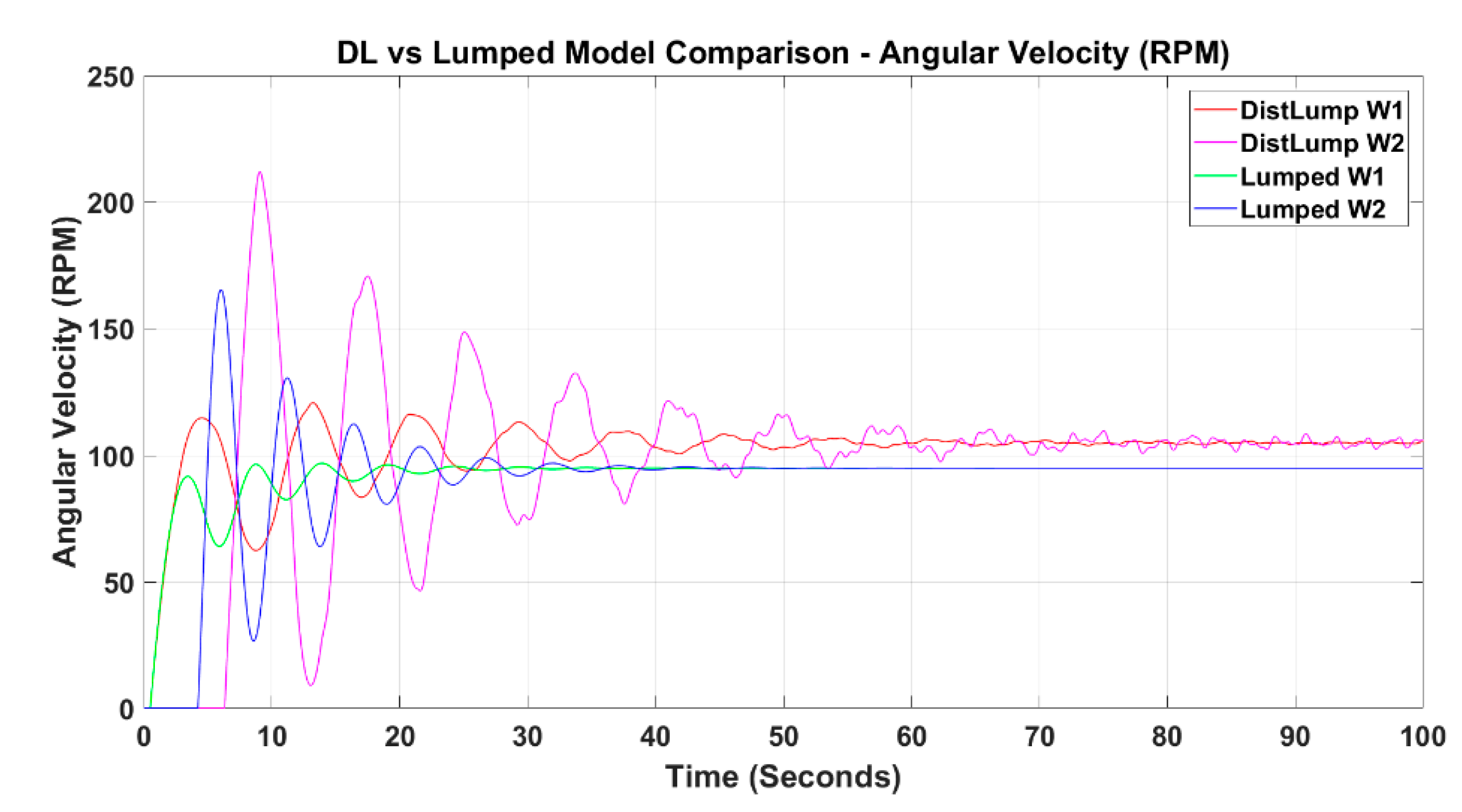
The simulations were performed with a drill pipe length of 2000 m using the variable parameters in Table 1. The angular velocity for the two models is shown in RPM in Figure 10. The graph helps to observe the critical speed of both models. The critical speed of the lumped model was lower than the critical velocity of the D–L model. For the lumped model, the critical speed was 95 RPM when the torque of the rotary table () was 13,470 Nm. For the D–L model, the critical speed was 106 RPM when the torque of the rotary table was 13,650 Nm.
The two models were tested at a lower speed where the stick-slip could initially be observed. Figure 11 shows the lower speed limit at which both models could detect the stick-slip. For the lumped model, when the rotating speed dropped to below 30 RPM, it went directly to 0 RPM without showing stick-slip. The input torque at 30 RPM was 9750 Nm, and as soon as the torque dropped below this value, the rotating speed became 0 RPM. On the other hand, the stick-slip at the D–L model occurred at an average speed of 22 RPM, where the input torque at that time was 9425 Nm. When the torque dropped below 9250 Nm, the rotating speed became 0 RPM.
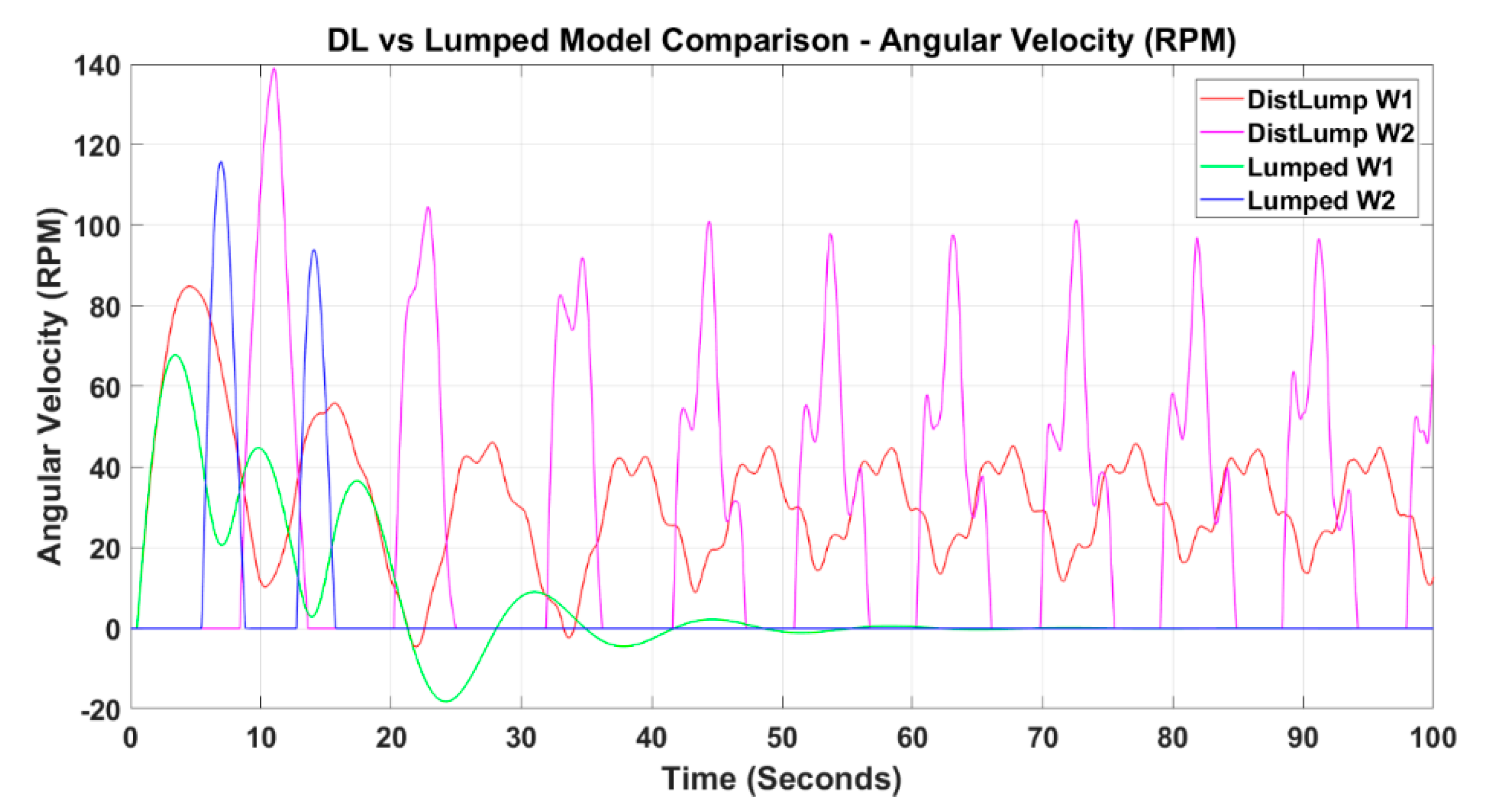
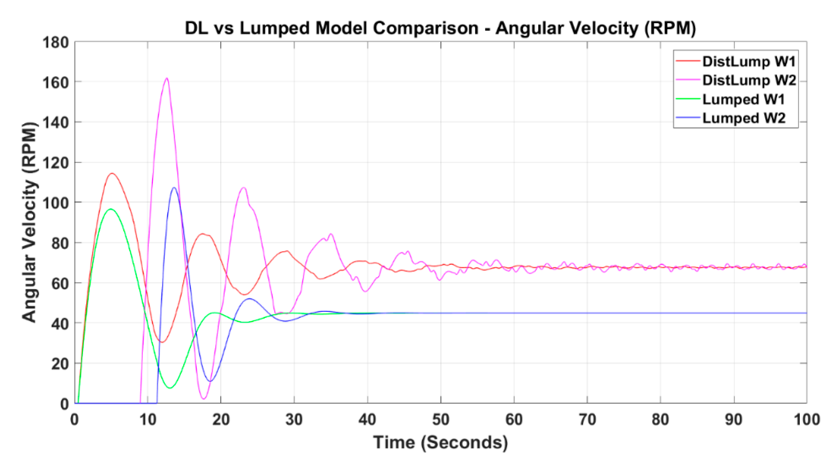
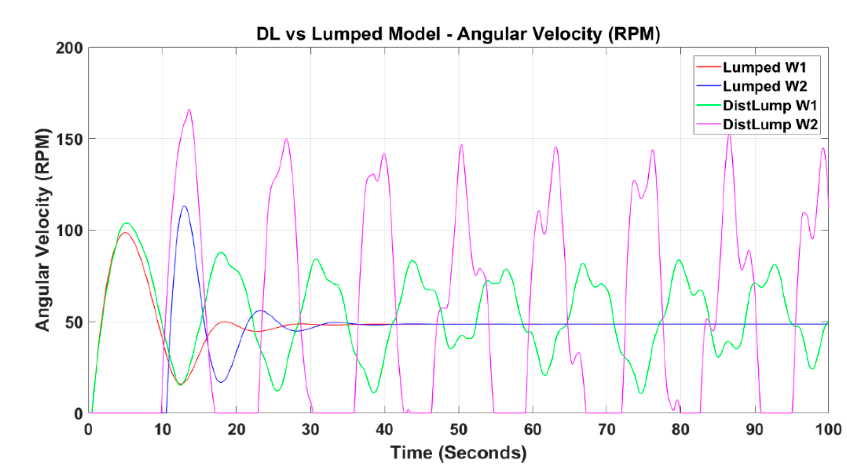
Figure 12 shows the angular velocity of the rotary table () and the drill bit () from the two models. Both models were set to run at the same angular velocity of 50 RPM, which was the desired speed of drilling. The difference between the two models at this speed could be clearly observed. By comparing the drill bit’s angular velocity in both models, it could be seen that the angular velocity in the D–L model fluctuated between zero and non-constant upper values (130, 140, 160, 180 RPM, etc.). The fluctuation range varied as the simulation time increased or decreased. On the other hand, the angular velocity of the drill bit () fluctuated between 0 RPM and a constant upper value of 150 RPM. Fluctuation was also observed in the curve of both angular velocities ( and ) from the D–L model. This behavior was not seen in the lumped model because its angular velocities had a smooth curve. Another important difference between the two models was that they had an unequal number of stick-slip vibrations. The numbers of stick-slip vibrations for the D–L and lumped models were 11 and 17. This number depended on the used parameters and simulation time.
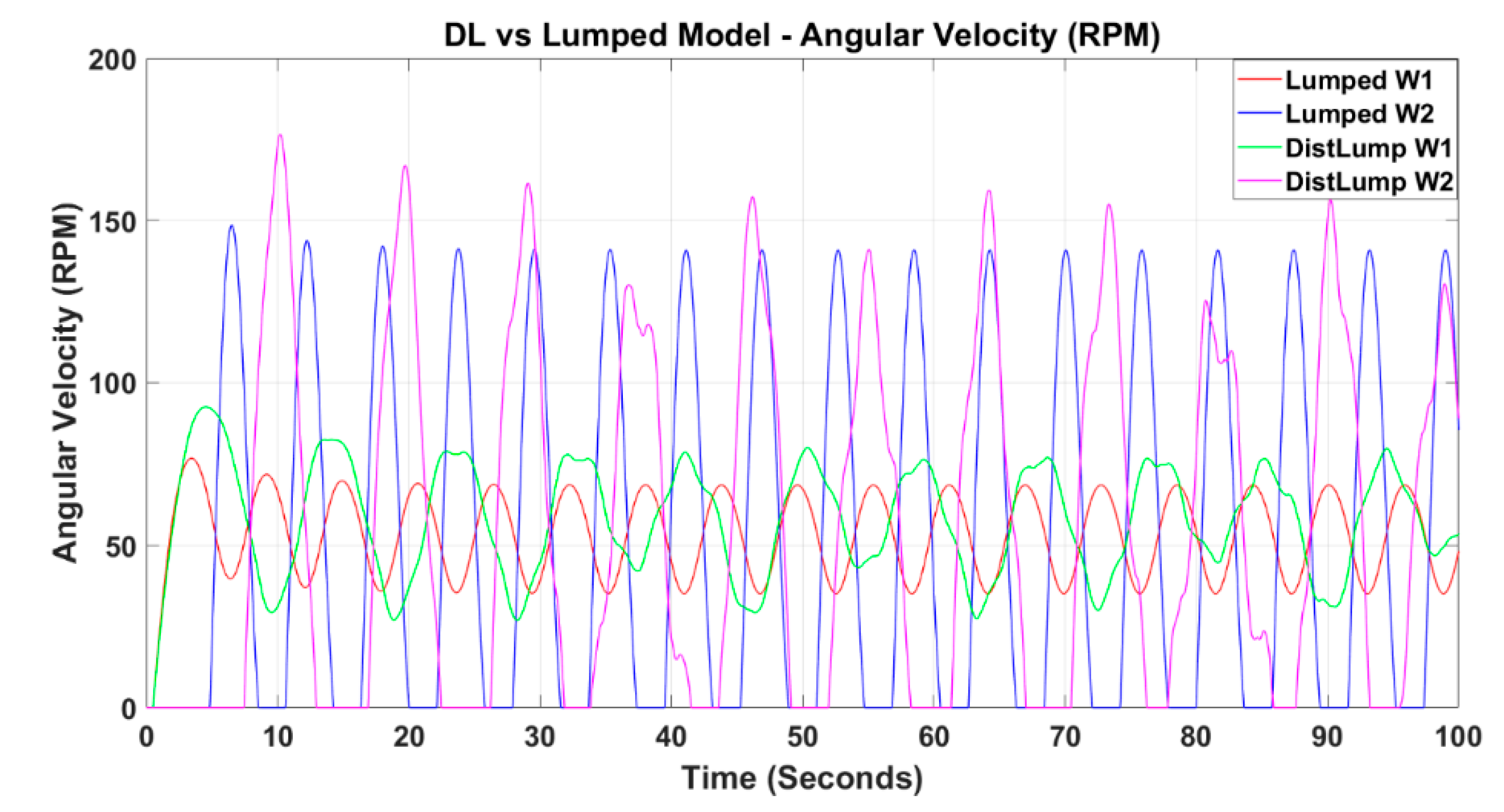
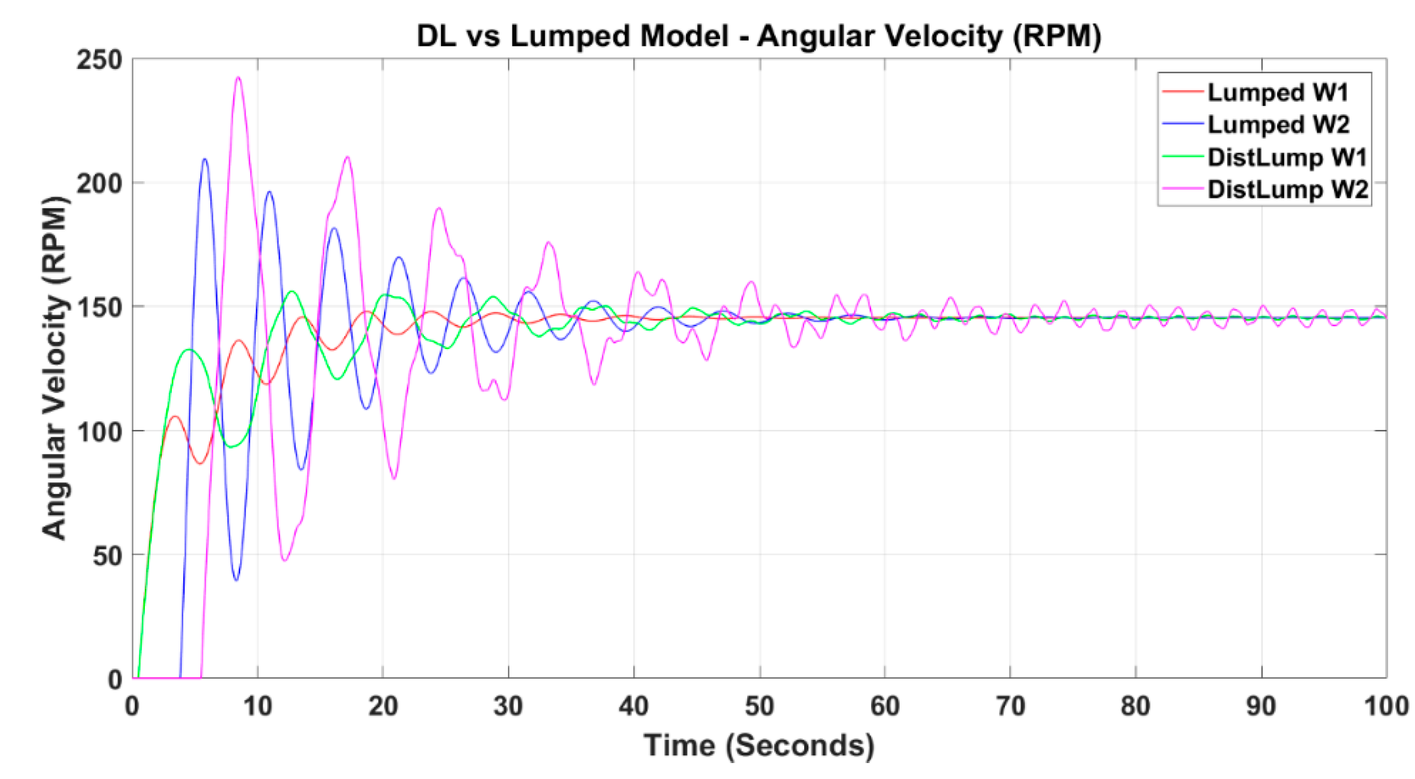
Figure 13 shows the behaviour of both models at the same angular velocity of 145 RPM. The input torque was different for each model. To reach this speed, the input torque for the lumped model was 14,980 Nm, and it was 14,350 Nm for the D–L model.
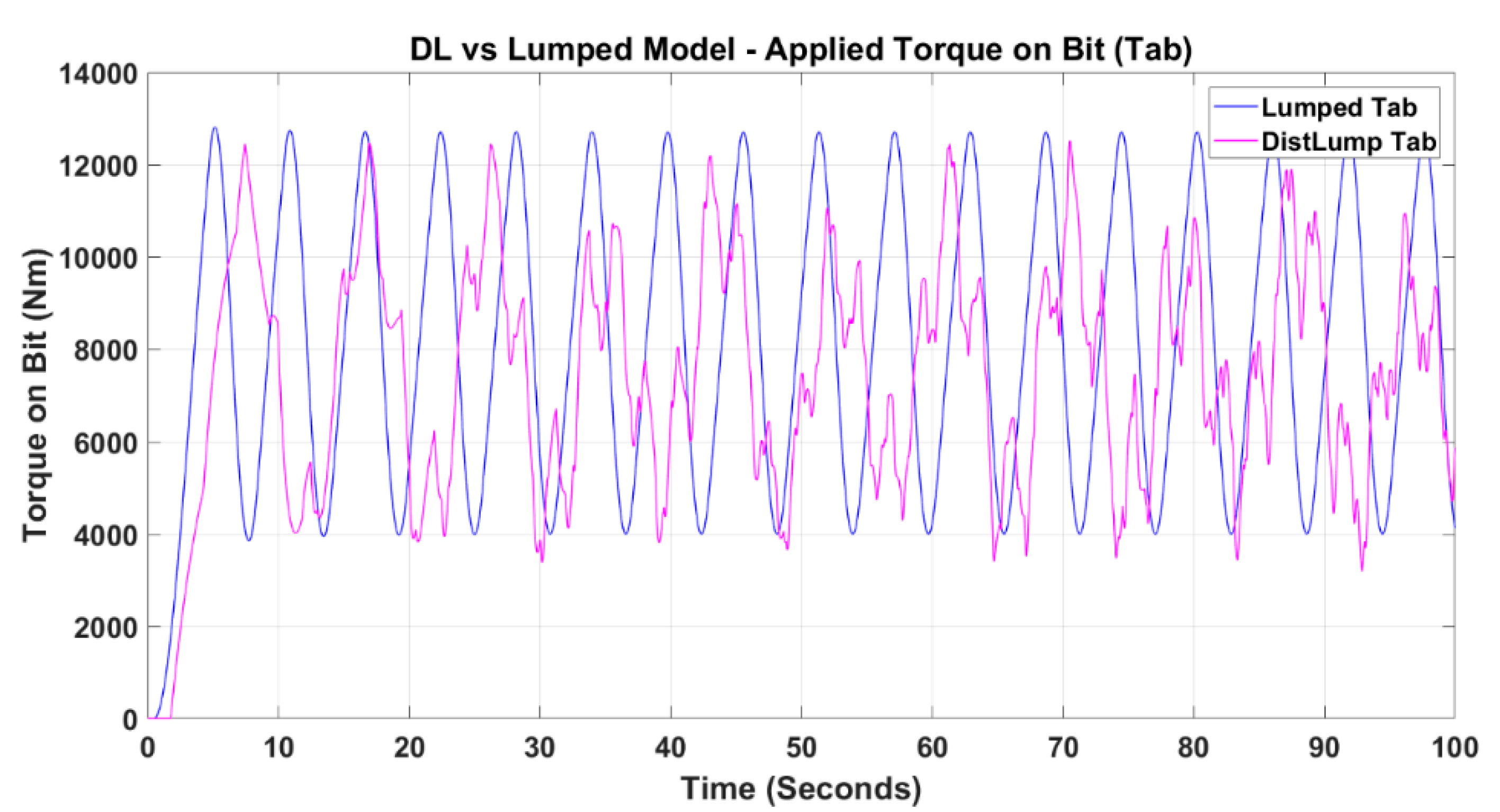
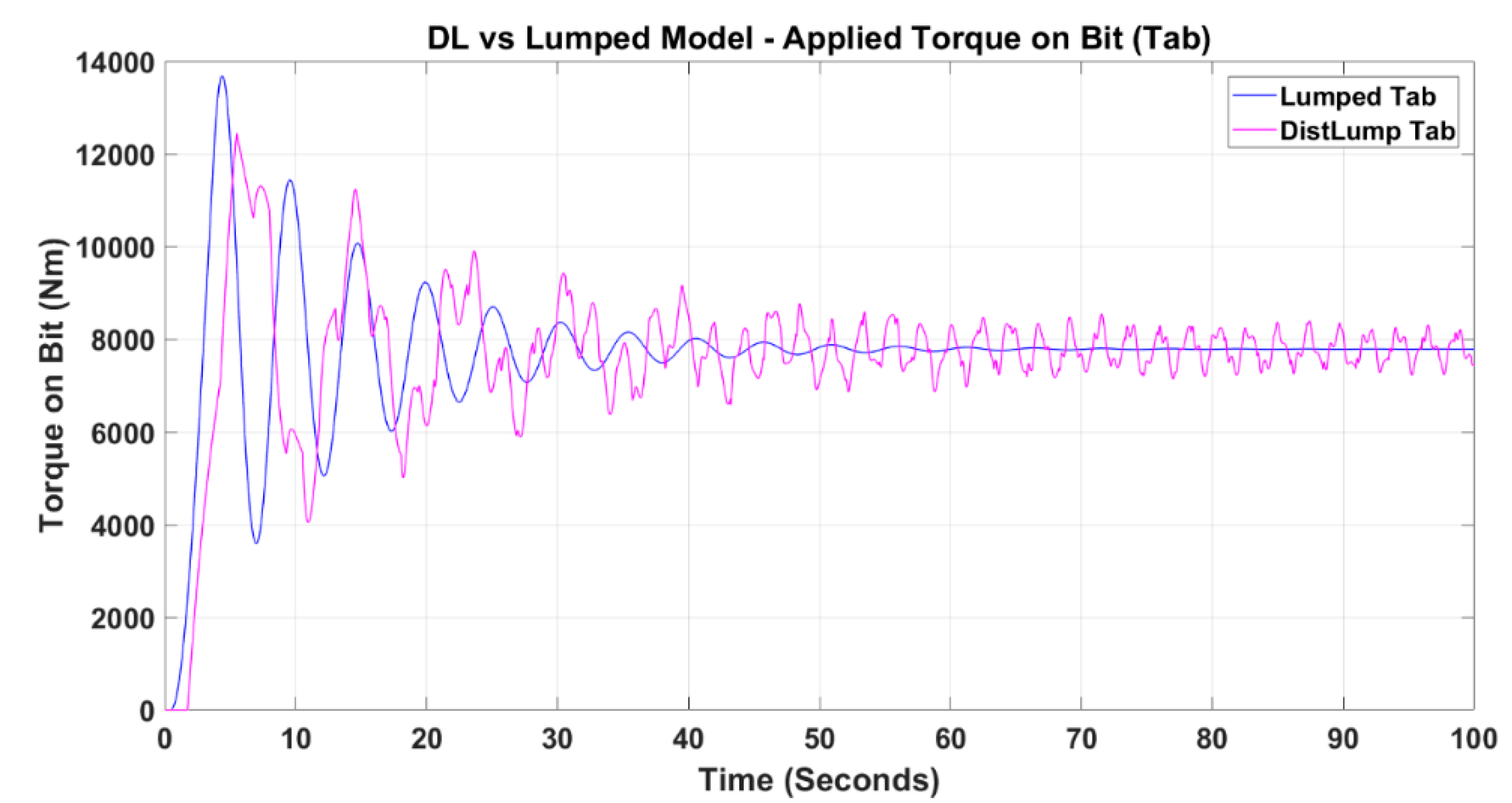
Figure 14 and Figure 15 show comparisons of the applied torque on the bit () of the two models at the desired speed of 50 RPM and the critical speed, respectively. The obtained torque from the D–L model appeared as an irregular shape, while the applied torque in the lumped model fluctuated smoothly. Both applied torques () fluctuated constantly between 4000 and 13,000 Nm. In Figure 14, the applied torque on bit () is shown for both models at the critical speed of 145 RPM. The in both models overcame the static friction () and continued with Coulomb friction torque (). For a drill bit to start moving, the applied torque on the bit must overcome the .
7.3. Simulation for Drill Pipe Length of 5700 m
Here, simulations were done for a drill pipe length of 5700 m as the drilling process moved deeper. When the length of the drill pipe increased, the torsional stiffness decreased, which may have led to the increment of the stick-slip vibrations. The simulations for this length of drill pipe were done using the variable parameters presented in Table 2.
Figure 16 shows the critical speed of the two models. From the figure, it can be observed that the critical speed of the two models was different. For the lumped model, the critical speed was 45 RPM at an input torque () of 10,150 Nm, while the critical speed for the D–L model was 68 RPM at an input torque of 11,500 Nm.
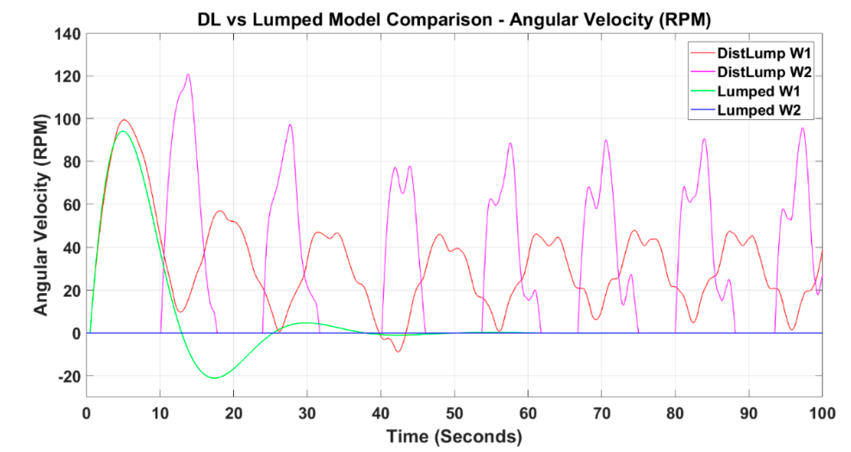
Figure 17 shows a comparison of the two models at the desired speed (50 RPM). In Figure 17, it can be observed that the difference between the two models increased. The lumped model had an angular velocity of 50 RPM that, compared with the real measurements presented in Figure 9 [30], was not correct because at this pipe length and 50 RPM, a stick-slip phase should have occurred. The D–L model showed stick-slip vibrations under these conditions.
Figure 18 shows the angular velocity of the two models at their minimum speed. It can be see that the lumped model failed to show any stick-slip vibrations at low speeds. The angular velocity of the lumped model became 0 RPM when the input torque at the rotary table was equal to 10,150 Nm. This was in contrast with the experiences of drillers and the scientific fact that stick-slip vibrations increase as the drill pipe length increases under the same operating conditions. On the other hand, the stick-slip vibrations in the D–L model occurred at an average speed of 20 RPM when the input torque at that time was 9975 Nm.
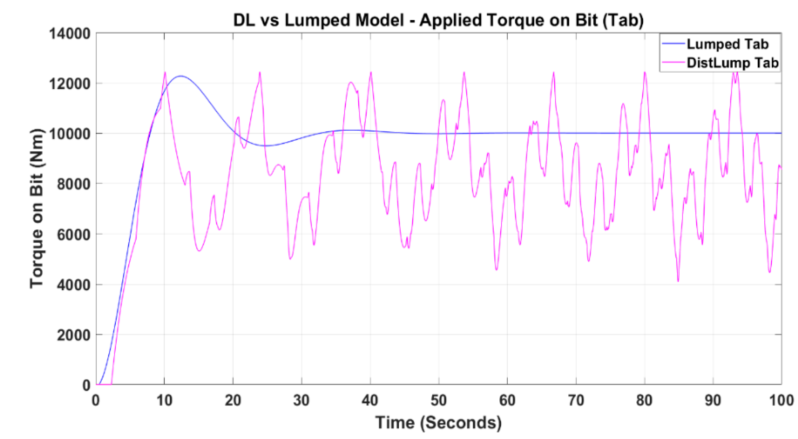
Figure 19 and Figure 20 show comparisons of the applied torque on bit () of the two models at the desired and critical speeds, respectively. From the figure, it can be seen that the applied torque on the bit obtained from the D–L model appeared as an irregular shape, while the line shape was smooth in the lumped model. The applied torque of the two models was very different. In the lumped model, the applied torque fluctuated for a small period in the beginning and then moved constantly in . This did not happen with the D–L model. For the D–L model, the applied torque on bit fluctuated constantly between 5000 and 12,200 Nm.
7.4. Simulation for Drill Pipe Length of 7500 m
As the drilling process continues to penetrate a dipper, the behaviour of the process changes. Here, simulations were done for a drill pipe length of 7500 m. Table 3 shows the equivalent parameters for this drill pipe length.
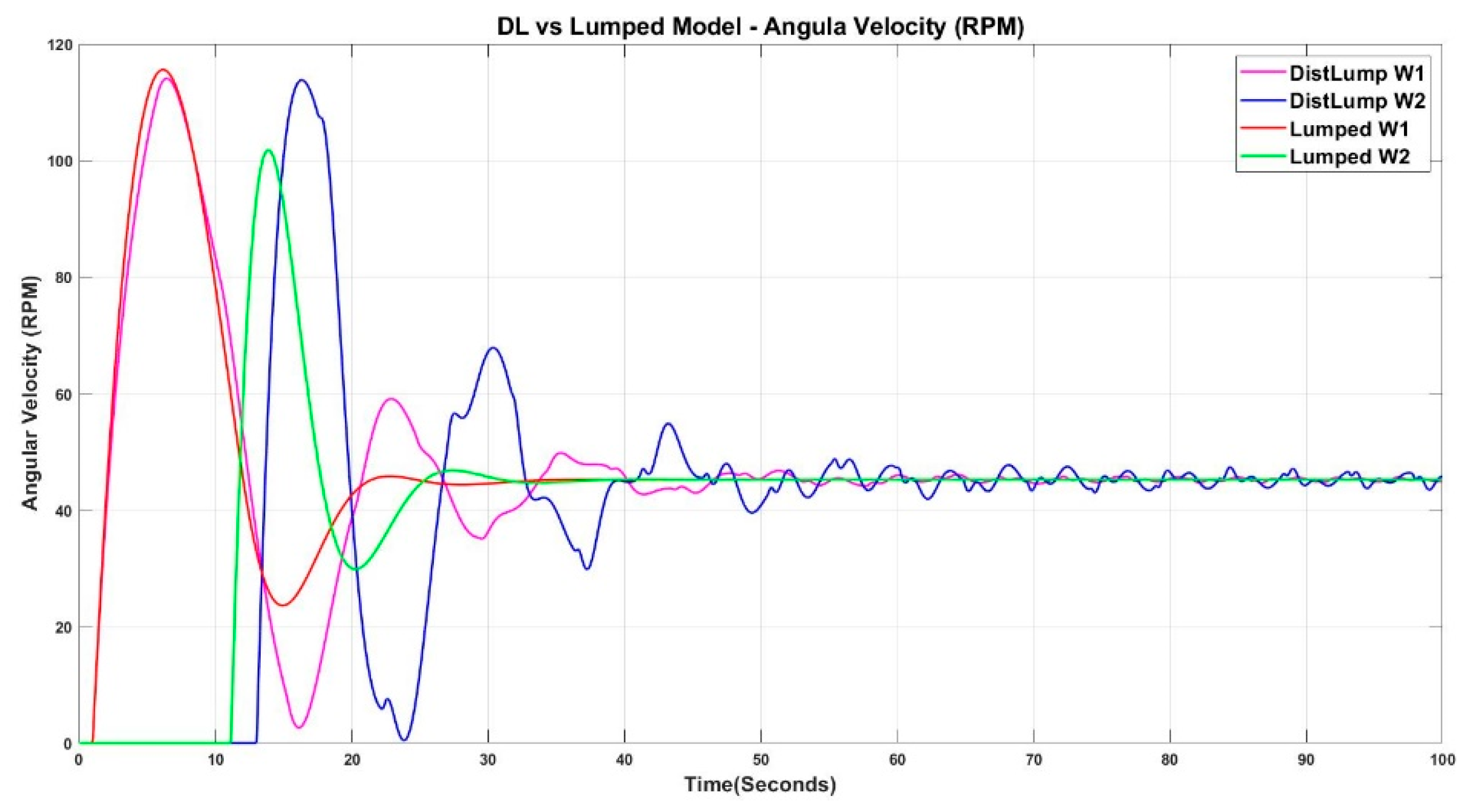
As can be seen in Figure 20, the critical speed changed significantly for both models. The new critical speed for both models was 45 RPM at . The D–L model initially just passed the stick-slip phase but, after few seconds, continued with an angular velocity of around 45 RPM. On the other hand, the lumped model did not show stick-slip vibrations, which was wrong.
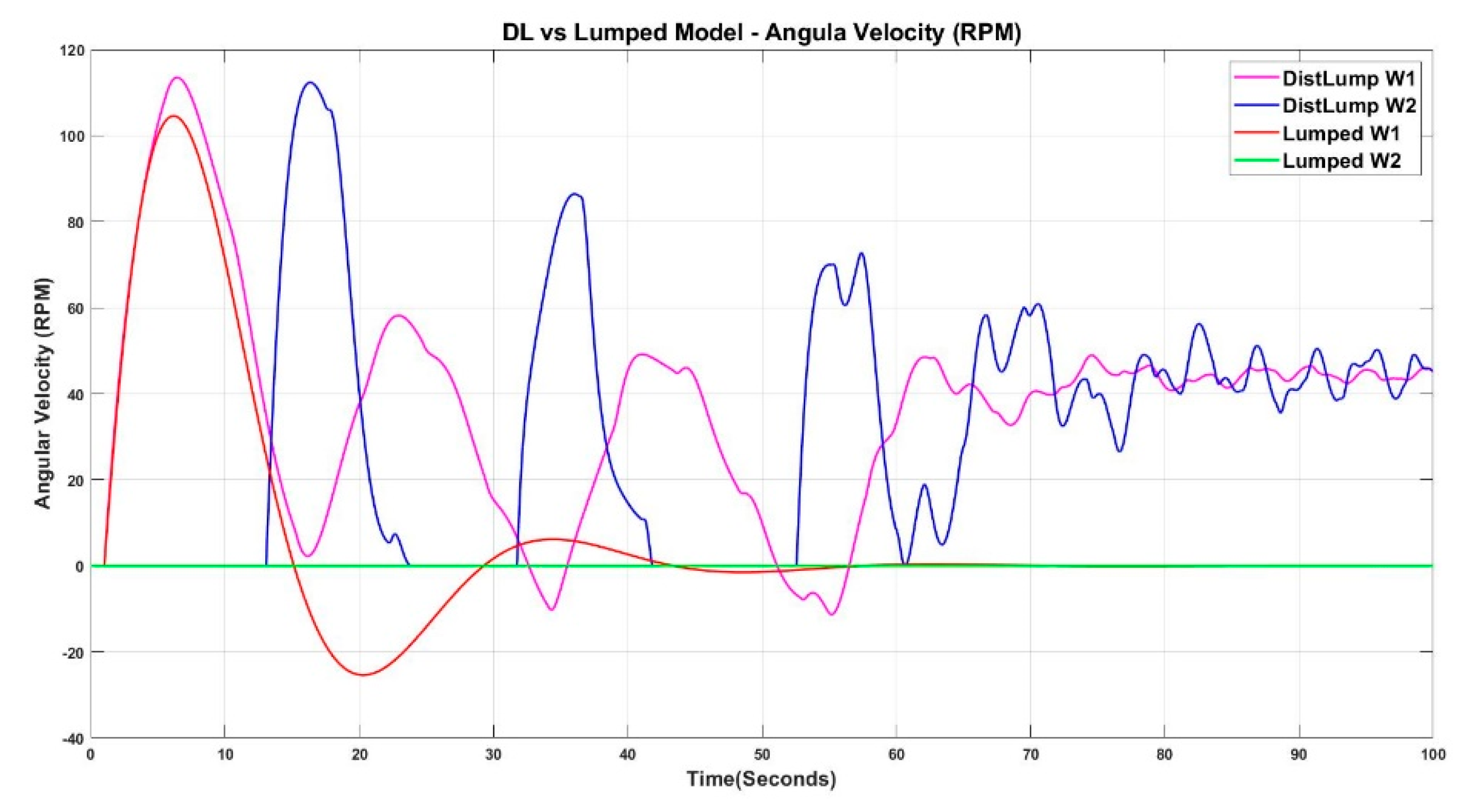
Figure 21 shows a comparison of the angular velocities obtained from both models. When the torque of the rotary table dropped to 10,250 Nm, the D–L model showed a transition from the slip phase to the stick-slip phase. The stick-slip phase fluctuated from 0 to 110 RPM. As the torque decreased, the angular velocity for the lumped model dropped to 0 RPM without going through the stick-slip phase. This was a weakness for the lumped model because it could not show stick-slip vibrations with longer drill pipes.
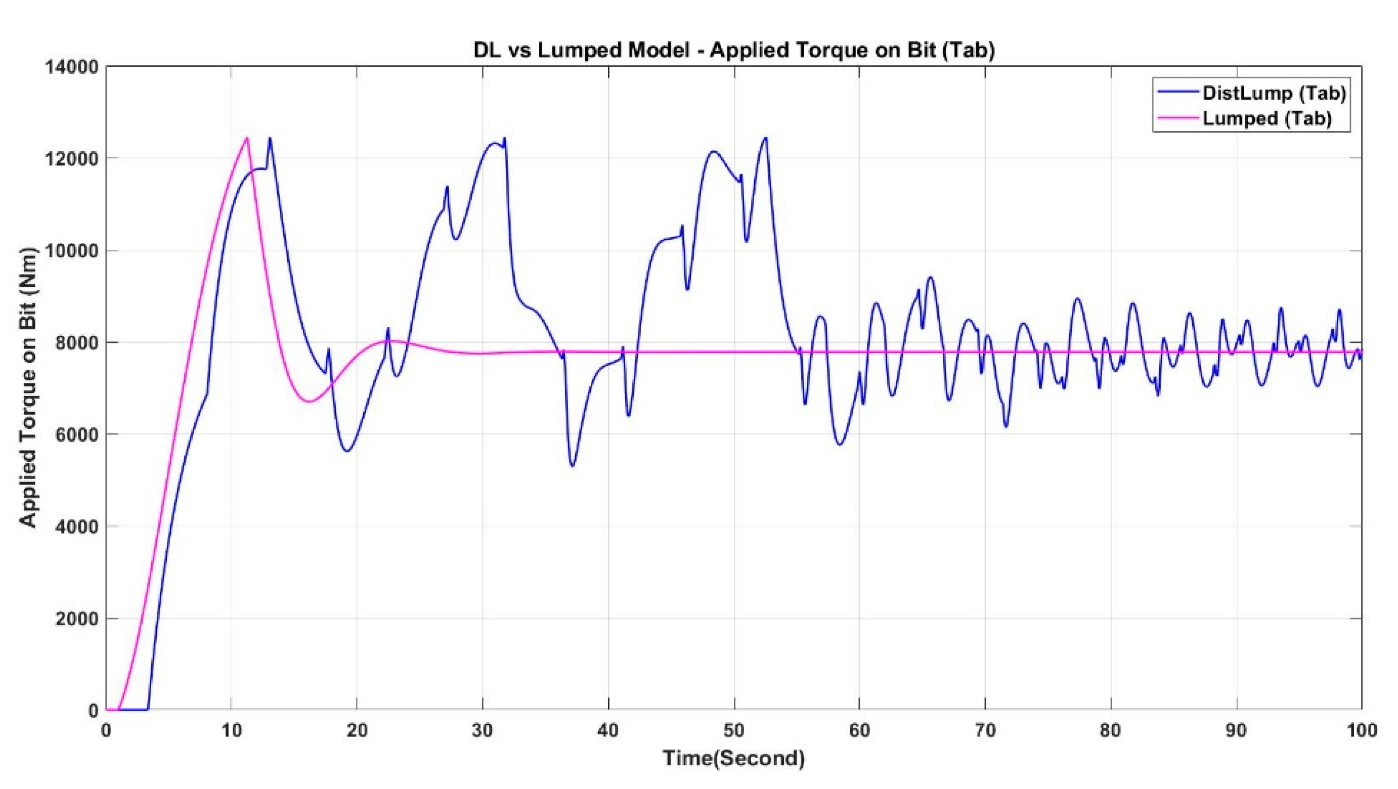
Figure 22 shows a comparison of the applied torque on the bit Tab of the two models at the desired speed. From the figure, it can be seen that the applied torque on the bit obtained from the D–L model appeared as an irregular shape, while the line shape was smooth in the lumped model. The applied torque of the two models was different. In the lumped model, the applied torque at the beginning went to the static friction torque (12,446) before returning immediately and continuing with Coulomb friction torque. The applied torque on the bit in the D–L model was initially (for about 60 s) fluctuating between 6000 and 12,446 Nm, and then, with small fluctuations, became continuous with Coulomb friction torque.
8. Conclusions
In this work, two models of a simple oil well drill system—a pure lumped model and a distributed–lumped model (hybrid model)—were created and validated. A comparison of the D–L and lumped versions was shown. Our study confirmed that the results were identical to an actual sample. In contrast, the D–L model was more precise, particularly for long strings. Since the lumped model passed from 50 to 0 RPM with a pipe length equal to 7500 m without sticking out of the slip step, the D–L model was more vulnerable to the slip of the pipe.
In the D–L model, the stick-slip vibrations behave differently than in the lumped model due to their strength. As the duration increased, the amplitude of the vibrations obtained from the D–L model increased. In the lumped model, where the amplitude of the vibrations remained the same, this did not happen. The applied torque was compared for the two models, and it was found that as the length of the drill pipe increased, the difference between them did as well.
For all three lengths, the applied torque obtained by the lumped model was constant (2000, 5700, and 7500 m). On the other hand, the applied torque on the bit obtained from the D–L model was different for all three lengths. As the length increased, the fluctuation of the applied torque in the D–L model increased, which was a result that was similar to an actual calculation found in the literature review.
The simulations were done based on real parameters found in [1,30,31]. Using these parameters, the results from the presented lumped and D–L models were able to be compared with other case studies and real measurements. Table A1 in Appendix A shows the parameters that were used for the validation of the models. These parameters remained constant for all drill pipe lengths. These parameters changed as the drill pipe length changed.
Author Contributions
Writing—original draft, P.A.; Writing—review & editing, Y.H. All authors have read and agreed to the published version of the manuscript.
Funding
This research received no external funding.
Conflicts of Interest
The authors declare no conflict of interest.
Nomenclature
| Capacitance per unit length | |
| Coefficient damping of bearing on the motor side | |
| Coefficient damping of bearing on the load side | |
| Equivalent viscous damping of the drive system | |
| Equivalent viscous damping coefficient along the drill pipe | |
| Damping coefficient of the drill pipe per unit length | |
| Equivalent viscous damping of the bottom hole assembly | |
| Outer diameter of the drill pipe | |
| Inner diameter of the drill pipe | |
| Outer diameter of the drill collar | |
| Inner diameter of the drill collar | |
| Outer diameter of the HWDP | |
| Inner diameter of the HWDP | |
| Conductance per unit length | |
| Shear modulus of steel | |
| Shear modulus of distributed shaft | |
| Current of armature of the motor | |
| Current at distance x and time t | |
| Inertia of distributed shaft | |
| Mass moment of inertia of the motor | |
| Mass moment of inertia of the rotary table | |
| Equivalent mass moment of inertia at motor side | |
| Equivalent mass moment of inertia of the BHA | |
| Mass moment of inertia of the drill string | |
| Mass moment of inertia of the HWDP | |
| Mass moment of inertia of the drill pipe | |
| Mass moment of inertia of the drill collar | |
| Mass moment of inertia of distributed shaft | |
| Mass moment of inertia of load | |
| Shaft polar moment of inertia | |
| The emf constant | |
| Motor constant related to physical properties of the motor | |
| Equivalent torsional stiffness of the drill pipe | |
| Inductance per unit length of electrical transmission line | |
| Armature inductance of the motor | |
| Length of drill pipe | |
| Length of HWDP | |
| Length of torsional distributed shaft | |
| A combined gear ratio of gear box and bevel gear | |
| Armature resistance of the motor | |
| Radius of shaft | |
| Radius of the bit | |
| Resistance per unit length | |
| Torque of motor | |
| Torque of the rotary table | |
| Torque on the bit (TOB) | |
| Viscosity damping torque over the BHA | |
| Friction torque on the bit | |
| External torque applied by drill string on the bit | |
| Static friction torque on the bit | |
| Sliding friction torque (cutting torque) | |
| Input torque to distributed shaft from a prime mover | |
| Input torque to drill pipe from a rotary table | |
| Output torque from distributed shaft to load | |
| Output torque from drill pipe to the BHA | |
| Back electric motive force (back-emf) of armature | |
| Supply armature voltage | |
| Voltage at distance x and time t | |
| Weight on a bit (WOB) | |
| Limit velocity interval | |
| Shear strain | |
| Positive constant defining the decaying velocity of | |
| Propagation constant of the electrical transmission line | |
| Propagation constant of the distributed | |
| Characteristic impedance of electrical transmission line | |
| Characteristic impedance of distributed shaft | |
| Characteristic impedance of the drill pipe | |
| Friction coefficient at the bit | |
| Coulomb friction coefficient | |
| Static friction coefficient | |
| Angular displacement of the motor | |
| Angular displacement of the rotary table | |
| Angular displacement of the bit | |
| Angle of twist | |
| Density of steel | |
| Density of distributed shaft | |
| Angular velocity of the motor shaft | |
| Angular velocity of the rotary table | |
| Angular velocity of the bit | |
| Angular velocity at the inlet of a distributed shaft | |
| Angular velocity at the outlet of a distributed shaft |
Appendix A

Table A1.
Constant parameters of the drilling system.
| Name | Symbol | Value | Units |
|---|---|---|---|
| Shear Modulus of Steel | N/m2 | ||
| Density of Steel | Kg/m2 | ||
| Radius of Drill Bit | |||
| Weight on Bit | |||
| Static Friction Torque on Bit | 12,446 | ||
| Coulomb Friction Torque on Bit | |||
| Length of the BHA | |||
| Length of HWDP | |||
| Outer Diameter of Drill Pipes | |||
| Inner Diameter of Drill Pipes | |||
| Outer Diameter of Drill Collar | |||
| Inner Diameter of Drill Collar | |||
| Outer Diameter of HWDP | |||
| Inner Diameter of HWDP | |||
| Gear Ratio | |||
| Inertia Mass Moment of Motor | Kgm2 | ||
| Inertia Mass Moment of Rotary Table | |||
| Inertia Mass Moment of Drive System | Kgm2 | ||
| Equivalent Mass Moment of Inertia of the BHA | Kgm2 | ||
| Equivalent Damping Coefficient of Drive System | Nms/rad | ||
| Propagation Constant of Drill Pipe | s/m | ||
| Static Friction Coefficients | |||
| Coulomb Friction Coefficients | |||
| Decaying Constant | |||
| Limit Velocity Interval | RPM | ||
| Inductance of Motor | |||
| Resistance of Motor | |||
| Constant of Motor | |||
| Emf Constant | |||
| Characteristic Impedance of Drill Pipe |
References
- Yigit, A.S.; Christoforou, A.P. Fully coupled vibrations of actively controlled drillstrings. J. Sound Vib. 2003, 267, 1029–1045. [Google Scholar] [CrossRef]
- Sahebkar, S.M.; Ghazavi, M.R.; Khadem, S.E.; Ghayesh, M.H. Nonlinear vibration analysis of an axially moving drillstring system with time dependent axial load and axial velocity in inclined well. Mech. Mach. Theory 2011, 46, 743–760. [Google Scholar] [CrossRef]
- Depouhon, A.; Detournay, E. Instability regimes and self-excited vibrations in deep drilling systems. J. Sound Vib. 2014, 333, 2019–2039. [Google Scholar] [CrossRef] [Green Version]
- Macdonald, K.A.; Bjune, J.V. Failure analysis of drillstrings. Eng. Fail. Anal. 2007, 14, 1641–1666. [Google Scholar] [CrossRef]
- Macdonald, K.A. Failure analysis of drillstring and bottom hole assembly components. Eng. Fail. Anal. 1994, 1, 91–117. [Google Scholar] [CrossRef]
- Tinivella, U.; Giustiniani, M. Numerical simulation of coupled waves in borehole drilling through a BSR. Mar. Pet. Geol. 2013, 44, 34–40. [Google Scholar] [CrossRef]
- Dugundji, J.; Mukhopadhyay, V. Lateral Bending-Torsion Vibrations of a Thin Beam Under Parametric Excitation. J. Appl. Mech. 1973, 40, 693–698. [Google Scholar] [CrossRef]
- Vielsack, P. Lateral bending vibrations of a beam with small pretwist. Eng. Struct. 2000, 22, 691–698. [Google Scholar] [CrossRef]
- Yigit, A.S.; Christoforou, A.P. Coupled Torsional and Bending Vibrations of Actively Controlled Drillstrings. J. Sound Vib. 2000, 234, 67–83. [Google Scholar] [CrossRef]
- Zamanian, M.; Khadem, S.E.; Ghazavi, M.R. Stick-slip oscillations of drag bits by considering damping of drilling mud and active damping system. J. Pet. Sci. Eng. 2007, 59, 289–299. [Google Scholar] [CrossRef]
- Jansen, J.D.; Van Den Steen, L. Active damping of self-excited torsional vibrations in oil well drillstrings. J. Sound Vib. 1995, 179, 647–668. [Google Scholar] [CrossRef]
- Rajnauth, J.; Jagai, T. Reduce Torsional Vibrations and Improve Drilling Operations. Int. J. Appl. Sci. Technol. 2012, 2, 109–122. [Google Scholar]
- Whalley, R. Interconnected spatially distributed system. Trans. Inst. Meas. Control 1990, 12, 262–270. [Google Scholar] [CrossRef]
- Russer, P.; Russer, J.A. Application of the Transmission Line Matrix (TLM) method to EMC problems. In Proceedings of the 2012 Asia-Pacific Symposium on Electromagnetic Compatibility, Singapore, 21–24 May 2012; pp. 141–144. [Google Scholar]
- Hoefer, W.J.R. The Transmission-Line Matrix Method—Theory and Applications. IEEE Trans. Microw. Theory Tech. 1985, 33, 882–893. [Google Scholar] [CrossRef] [Green Version]
- Baker, R. A Primer of Oilwell Drilling: A Basic Text of Oil and Gas Drilling, 6th ed.; Petroleum Extension Service, Continuing & Extended Education, University of Texas at Austin: Austin, TX, USA, 2001. [Google Scholar]
- Bommer, P. A Primer of Oilwell Drilling: A Basic Text of Oil and Gas Drilling, 7th ed.; Petroleum Extension Service, Continuing & Extended Education, University of Texas at Austin: Austin, TX, USA, 2008. [Google Scholar]
- Bowman, I. Well-Drilling Methods, Water-Supply Paper-257; Government Printing Office: Washington, DC, USA, 1911.
- Mitchell, R.F.; Miska, S.Z. Fundamental of Drilling Engineering, SPE Textbook Series; Society of Petroleum Engineers: Oklahoma City, OK, USA, 2011; Volume 12, ISBN 9781555632076. [Google Scholar]
- Baker, H. Oil Field Familiarization: Training Guide; Baker Hughes INTEQ: Houston, TX, USA, 1996. [Google Scholar]
- Brett, J.F. The Genesis of Torsional Drillstring Vibrations, Society of Petroleum Engineers, SPE Drilling Engineering; Society of Petroleum Engineers: Oklahoma City, OK, USA, 1992; pp. 168–174. [Google Scholar]
- Navarro-López, E.M.; Suarez, R. Practical approach to modelling and controlling stick-slip oscillations in oilwell drillstrings. In Proceedings of the IEEE International Conference on Control Applications, Institute of Electrical and Electronics Engineers (IEEE), Taipei, Taiwan, 2–4 September 2004; Volume 2, pp. 1454–1460. [Google Scholar]
- Brett, J.F. The Genesis of Bit-Induced Torsional Drillstring Vibrations. SPE Drill. Eng. 1992, 7, 168–174. [Google Scholar] [CrossRef]
- Navarro-Lopez, E.M.; Suarez, R. Modelling and Analysis of Stick-Slip Behaviour in a Drillstring Under Dry Friction. In Proceedings of the Congress of the Mexican Association of Automatic Control; 2004; Volume 1, pp. 330–335. Available online: https://d1wqtxts1xzle7.cloudfront.net/31021540/enavarro_amca04.pdf?1364097902=&response-content-disposition=inline%3B+filename%3DModelling_and_Analysis_of_Stick_slip_Beh.pdf&Expires=1605156926&Signature=LviT~TRxy4IRtGCEy1ujSp-3-XviugLTC8NLZhugqzZZ2FKeG5Bbv-iOP0HWgdpt0hMnKceW9lvAxri9FrUGQQORZ71UhHbrvxCAscAT5Rf~EqyLFJPwIObZUPZfPqQVhFyn~EVX649GhjkNLhSAEQItk9PiA16xqRtYuP5XnKa3-96qfBN8GDeu6Mc8WqblVKAfXvv3bVw5T3f3I~lvv9-6~Xw8IEyjrMf1Nu8S9cHOms6x3xyeyVzb90k-TB3n5uKfSs-2EsqTywpc7TiKdwiWvHz94onY3G8VPsu0MoRmjX-YQGBHblOXhVYYPGPRBVv1W11H0XENamP-qTb7eQ__&Key-Pair-Id=APKAJLOHF5GGSLRBV4ZA (accessed on 1 June 2020).
- Armstrong-Hélouvry, B.; Dupont, P.; Canudas-De Wit, C. A survey of models, analysis tools and compensation methods for the control of machines with friction. Automatica 1994, 30, 1083–1138. [Google Scholar] [CrossRef]
- Márquez, M.B.S.; Boussaada, I.; Mounier, H.; Niculescu, S.-I. Analysis and Control of Oilwell Drilling Vibrations; Springer Science and Business Media LLC: Berlin/Heidelberg, Germany, 2015. [Google Scholar]
- Christopoulos, C. The Transmission-Line Modelling Method, Synthesis Lectures on Computational Electromagnetics; Morgan & Claypool. 2006. Available online: https://www.morganclaypool.com/doi/abs/10.2200/S00316ED1V01Y201012CEM027 (accessed on 1 June 2020).
- Whalley, R.; Ebrahimi, M.; Jamil, Z. The torsional response of rotor systems. Proc. Inst. Mech. Eng. J. Mech. Eng. Sci. 2005, 219, 357–380. [Google Scholar] [CrossRef] [Green Version]
- Pavone, D.R.; Desplans, J.P. Application of High Sampling Rate Downhole Measurements for Analysis and Cure of Stick-Slip in Drilling. Soc. Pet. Eng. 1994. [Google Scholar] [CrossRef]
- Jansen, J.D.; Van den Steen, L.; Zachariasen, E. Active Damping of Torsional Drillstring Vibrations With a Hydraulic Top Drive. SPE Drill. Complet. 1995, 10, 250–254. [Google Scholar] [CrossRef]
- Navarro-López, E.M.; Licéaga-Castro, E. Non-desired transitions and sliding-mode control of a multi-DOF mechanical system with stick-slip oscillations. Chaos Solitons Fractals 2009, 41, 2035–2044. [Google Scholar] [CrossRef]
Figure 1.
Interconnected distributed–lumped parameter system [13].
Figure 1.
Interconnected distributed–lumped parameter system [13].

Figure 2.
Schematic representation of onshore/land drilling rig.

Figure 3.
Schematic representation of the modelled drilling system used for the lumped model.

Figure 4.
Block diagram of the lumped model of a drilling system.

Figure 5.
An infinitesimal element of a transmission line for an electrical system.

Figure 6.
Twisting shaft with its sliced differential element of length dx.

Figure 7.
Distributed model of a torsional shaft block diagram.

Figure 8.
Block diagram of the distributed–lumped (D–L) model interconnection.

Figure 9.
The real measurement of stick-slip vibrations [29].
Figure 9.
The real measurement of stick-slip vibrations [29].

Figure 10.
Comparison between angular velocities obtained from the lumped and D–L models at critical speed for Ldp = 2000 m.
Figure 10.
Comparison between angular velocities obtained from the lumped and D–L models at critical speed for Ldp = 2000 m.

Figure 11.
Comparison between angular velocities obtained from the lumped and D–L models at low speed for Ldp = 2000 m.
Figure 11.
Comparison between angular velocities obtained from the lumped and D–L models at low speed for Ldp = 2000 m.

Figure 12.
Comparison between angular velocities obtained from the lumped and D–L models at 50 RPM for Ldp = 2000 m.
Figure 12.
Comparison between angular velocities obtained from the lumped and D–L models at 50 RPM for Ldp = 2000 m.

Figure 13.
Comparison of the lumped and D–L models’ behaviour at the same angular velocity at Ldp = 2000 m.
Figure 13.
Comparison of the lumped and D–L models’ behaviour at the same angular velocity at Ldp = 2000 m.

Figure 14.
Comparison between applied torque on bit obtained from the lumped and D–L models at 50 RPM for Ldp = 2000 m.
Figure 14.
Comparison between applied torque on bit obtained from the lumped and D–L models at 50 RPM for Ldp = 2000 m.

Figure 15.
Comparison between applied torque on bit obtained from the lumped and D–L models at critical speed for Ldp = 2000 m.
Figure 15.
Comparison between applied torque on bit obtained from the lumped and D–L models at critical speed for Ldp = 2000 m.

Figure 16.
Comparison between angular velocities obtained from the lumped and D–L models at critical speed for Ldp = 5700 m.
Figure 16.
Comparison between angular velocities obtained from the lumped and D–L models at critical speed for Ldp = 5700 m.

Figure 17.
Comparison between angular velocities obtained from the lumped and D–L models at 50 RPM for Ldp = 5700 m.
Figure 17.
Comparison between angular velocities obtained from the lumped and D–L models at 50 RPM for Ldp = 5700 m.

Figure 18.
Comparison between angular velocities obtained from the lumped and D–L models at minimum speed for Ldp = 5700 m.
Figure 18.
Comparison between angular velocities obtained from the lumped and D–L models at minimum speed for Ldp = 5700 m.

Figure 19.
Comparison between applied torque on bit obtained from the lumped and D–L models at 50 RPM for Ldp = 5700 m.
Figure 19.
Comparison between applied torque on bit obtained from the lumped and D–L models at 50 RPM for Ldp = 5700 m.

Figure 20.
Comparison between angular velocities obtained from the lumped and D–L models at 45 RPM for Ldp = 7500 m.
Figure 20.
Comparison between angular velocities obtained from the lumped and D–L models at 45 RPM for Ldp = 7500 m.

Figure 21.
Comparison between angular velocities obtained from the lumped and the D–L models at low velocity for Ldp = 7500 m.
Figure 21.
Comparison between angular velocities obtained from the lumped and the D–L models at low velocity for Ldp = 7500 m.

Figure 22.
Comparison between applied torque on bit obtained from the lumped and the D–L models at 45 RPM for Ldp = 7500 m.
Figure 22.
Comparison between applied torque on bit obtained from the lumped and the D–L models at 45 RPM for Ldp = 7500 m.

Table 1.
Variable Parameters of the drilling system with a length of drill pipe (Ldp) = 2000 m.
| Name | Symbol | Value | Units |
|---|---|---|---|
| Length of Drill Pipe | 2000 | m | |
| Viscous Damping along with Drill Pipe | 23 | Nms/rad | |
| Viscous Damping along with the bottom hole assembly (BHA) | 50 | Nms/rad | |
| Equivalent Inertia Mass Moment of Drill String | 540.6 | Kgm2 | |
| Drill Pipe Stiffness | 473 | Nms/rad | |
| Propagation Time Associated with Drill Pipe | 0.6281 | s |
Table 2.
Variable parameters for .
| Name | Symbol | Value | Units |
|---|---|---|---|
| Length of Drill Pipe | 5700 | m | |
| Viscous Damping along with Drill Pipe | 85 | Nms/rad | |
| Viscous Damping along with the BHA | 100 | Nms/rad | |
| Equivalent Inertia Mass Moment of Drill String | 655.6 | Kgm2 | |
| Drill Pipe Stiffness | 166 | Nms/rad | |
| Propagation Time Associated with Drill Pipe | 1.79 | s |
Table 3.
Variable parameters for Ldp = 7500 m.
| Name | Symbol | Value | Units |
|---|---|---|---|
| Length of Drill Pipe | 7500 | m | |
| Viscous Damping along Drill Pipe | 140 | Nms/rad | |
| Viscous Damping along the BHA | Ceb | 150 | Nms/rad |
| Equivalent Inertia Mass Moment of Drill String | Jes | 711.6 | Kgm2 |
| Drill Pipe Stiffness | Kdp | 126 | Nms/rad |
| Propagation Time Associated with Drill Pipe | td | 2.3553 | s |
Publisher’s Note: MDPI stays neutral with regard to jurisdictional claims in published maps and institutional affiliations. |
© 2020 by the authors. Licensee MDPI, Basel, Switzerland. This article is an open access article distributed under the terms and conditions of the Creative Commons Attribution (CC BY) license (http://creativecommons.org/licenses/by/4.0/).
Share and Cite
MDPI and ACS Style
Athanasiou, P.; Hadi, Y. Simulation of Oil Well Drilling System Using Distributed–Lumped Modelling Technique. Modelling 2020, 1, 175-197. https://0-doi-org.brum.beds.ac.uk/10.3390/modelling1020011
AMA Style
Athanasiou P, Hadi Y. Simulation of Oil Well Drilling System Using Distributed–Lumped Modelling Technique. Modelling. 2020; 1(2):175-197. https://0-doi-org.brum.beds.ac.uk/10.3390/modelling1020011
Chicago/Turabian StyleAthanasiou, Panagiotis, and Yaser Hadi. 2020. "Simulation of Oil Well Drilling System Using Distributed–Lumped Modelling Technique" Modelling 1, no. 2: 175-197. https://0-doi-org.brum.beds.ac.uk/10.3390/modelling1020011