
Modeling and Simulation of Head Trauma Utilizing White Matter Properties from Magnetic Resonance Elastography


1
Department of Mechanical Science & Engineering, University of Illinois at Urbana-Champaign, Urbana, IL 61801, USA
2
Beckman Institute and Institute for Condensed Matter Theory, University of Illinois at Urbana-Champaign, Urbana, IL 61801, USA
*
Author to whom correspondence should be addressed.
Modelling 2020, 1(2), 225-241; https://0-doi-org.brum.beds.ac.uk/10.3390/modelling1020014
Submission received: 15 July 2020
/
Revised: 8 December 2020
/
Accepted: 8 December 2020
/
Published: 14 December 2020
(This article belongs to the Section Modelling in Biology and Medicine)
Abstract
:Tissues of the brain, especially white matter, are extremely heterogeneous—with constitutive responses varying spatially. In this paper, we implement a high-resolution Finite Element (FE) head model where heterogeneities of white matter structures are introduced through Magnetic Resonance Elastography (MRE) experiments. Displacement of white matter under shear wave excitation is captured and the material properties determined through an inversion algorithm are incorporated in the FE model via a two-term Ogden hyper-elastic material model. This approach is found to improve model predictions when compared to experimental results. In the first place, mechanical response in the cerebrum near stiff structures such as the corpus callosum and corona radiata are markedly different compared with a homogenized material model. Additionally, the heterogeneities introduce additional attenuation of the shear wave due to wave scattering within the cerebrum.
1. Introduction
With approximately 2.8 million cases reported annually in the United States [1], traumatic brain injury (TBI)—commonly caused by a direct blow or impulse to the head—remains a pressing concern for study. Clinical results show that damage to the brain in blunt head injuries has a tendency to occur in regions with highly organized axon tracts such as the brainstem and corpus callosum [2,3,4,5,6,7]. These regions serve as pathways to other parts of the brain, meaning damage to them is potentially more dangerous. In this work, we introduce a heterogeneous material description of white matter structures to our high-resolution Finite Element (FE) model to account for the local differences in mechanical response between different regions of the brain.
The FE method is commonly used to determine the mechanical response of brain tissue in order to develop improved diagnostic tools and protective measures to reduce the prevalence of TBI. The accuracy of these FE models is highly dependent on the accuracy of the material model. To date, many finite element models have utilized mechanical properties homogenized over large portions of the brain, as reviewed in [8], thus ignoring potentially significant effects of local structures. In actuality, the tissues of the brain are heterogeneous, their constitutive response varying from location to location. This is most noticeable for white matter due to the presence of axons with diverse orientations. Overall, the shear stiffness of white matter is 1.2–2.6 times higher than that of gray matter [9]. Locally, white matter tracts, with highly oriented fibers such as the corpus callosum and corona radiata, have material properties different from other regions. Johnson et al. [10] determined that global—or averaged—white matter was softer on average than either the corpus callosum or the corona radiata. This can be explained by considering the structure of these regions. The corpus callosum provides more structural rigidity than the superficial white matter due to the presence of highly aligned fibers. The fan-like structure of the corona radiata exhibits similar behavior, but to a lesser degree as the fibers are not as highly aligned. As such, the corpus callosum was found to be approximately 11% stiffer than the corona radiata [10]. The brainstem is another structure with a high level of heterogeneity. Arbogast and Margulies [7] investigated the prevalence of trauma observed in the brainstem after head injuries. They determined that the brainstem was 80–100% stiffer than the cerebrum and concluded this regional stiffness—in addition to its anisotropic response and location as a narrow bridge between CNS regions—as the main reasons for the selective vulnerability of this region. FE models that utilize homogenized white matter material properties have no way to resolve these local features.
A very useful tool to measure heterogeneity in-vivo is the Magnetic Resonance Elastography (MRE) [11], where local mechanical properties of brain tissue are quantitatively determined by external actuation of the head to generate shear waves. This technique has been successfully applied to a variety of different applications: investigating decreases in whole-brain stiffness with age [12] and in neurodegenerative diseases [13]; measurement of tumor stiffness [14]; and as a marker for TBI severity [15]. MRE is applied as a three-step process beginning by first inducing shear waves in tissue with frequencies ranging from 50 to 500 Hz using an external driver [11]. Second, the waves are imaged using a phase-contrast MRI pulse sequence synchronized with the frequency of the applied vibration. Finally, the mechanical properties of the tissue are estimated by performing an inversion of the observed displacements using a viscoelastic material model, such as that presented by Van Houten et al. [16].
In this work we utilize our previously homogeneous FE model—presented and validated in our previous works [17,18,19]—and introduce a voxel-based heterogeneous material model using results from Johnson et al. [10]. Our previous model was homogeneous in the sense that properties were taken as location-independent within the white matter. The mechanical properties used in this work are now reconstructed at the same spatial resolution as the displacement data captured during the MRE process. The resulting finite element mesh has sufficient resolution to accurately capture the dynamic shear wave propagation during impacts, a necessary feature of computational mechanics models of TBI. To the best of our knowledge, this is the first attempt to include heterogeneity of brain tissue via MRE in a high-resolution FE model.
2. Model Formulation
2.1. MRE Acquisition and Inversion
The heterogeneous properties of the white matter are taken from the work by Johnson et al. [10]. A brief overview of the acquisition and inversion is presented here. A more detailed discussion of this process can be found in [20]. Shear waves are generated at a frequency of 50 Hz by placing the subject’s head on a custom cradle attached to an electromagnetic shaker via a rigid rod. The actuator imparts a nodding motion to the head, while the displacement data are captured via a Siemens 3T Allegra head-only scanner (Siemens Medical Solutions; Erlangen, Germany). A multi-shot MRE sequence utilizing spiral readout gradients [21] with periods matching that of the applied shear wave is developed to reduce errors during the inversion step. In total, the imaging volume comprises twenty axial slices of 2 mm thickness covering the ventricles, corpus callosum and corona radiata resulting in a mm isotropic spatial resolution for the reconstructed mechanical properties.
A nonlinear inversion (NLI) algorithm [16] is applied to estimate the material properties from the measured displacement data. The inversion is performed by minimizing the function
by iteratively updating the material property description, given by . Here, is the measured displacement amplitude at the location i; is the computed displacement amplitude sampled at the same point determined by a numerical model; and indicates the complex conjugate.
Following the development in [22], a Rayleigh damping model is used to represent the material response of brain tissue under time-harmonic conditions. The motion amplitude field u is calculated from Navier’s equation for an inhomogeneous, locally isotropic linear elastic medium
where is the first Lamé parameter; G is the second Lamé parameter, or shear modulus; is the density; and is the activation frequency. The Rayleigh damping model introduces the complex-valued shear modulus and densityas out to account for attenuation related to both elastic and inertial forces, where the imaginary shear modulus includes damping effects due to inertial forces. Including inertial damping effects—something that commonly used viscoelastic models do not include—allows for better characterization of material response when performing the inversion. We use the notation and to denote the storage and loss shear moduli, respectively, which are the real and imaginary part of the complex valued shear modulus
i being the imaginary unit. Due to the nearly incompressible nature of brain tissue, we assume that is very large compared to the shear modulus. The damping ratio
can be determined as well, which physically describes the level of motion attenuation in the tissue.
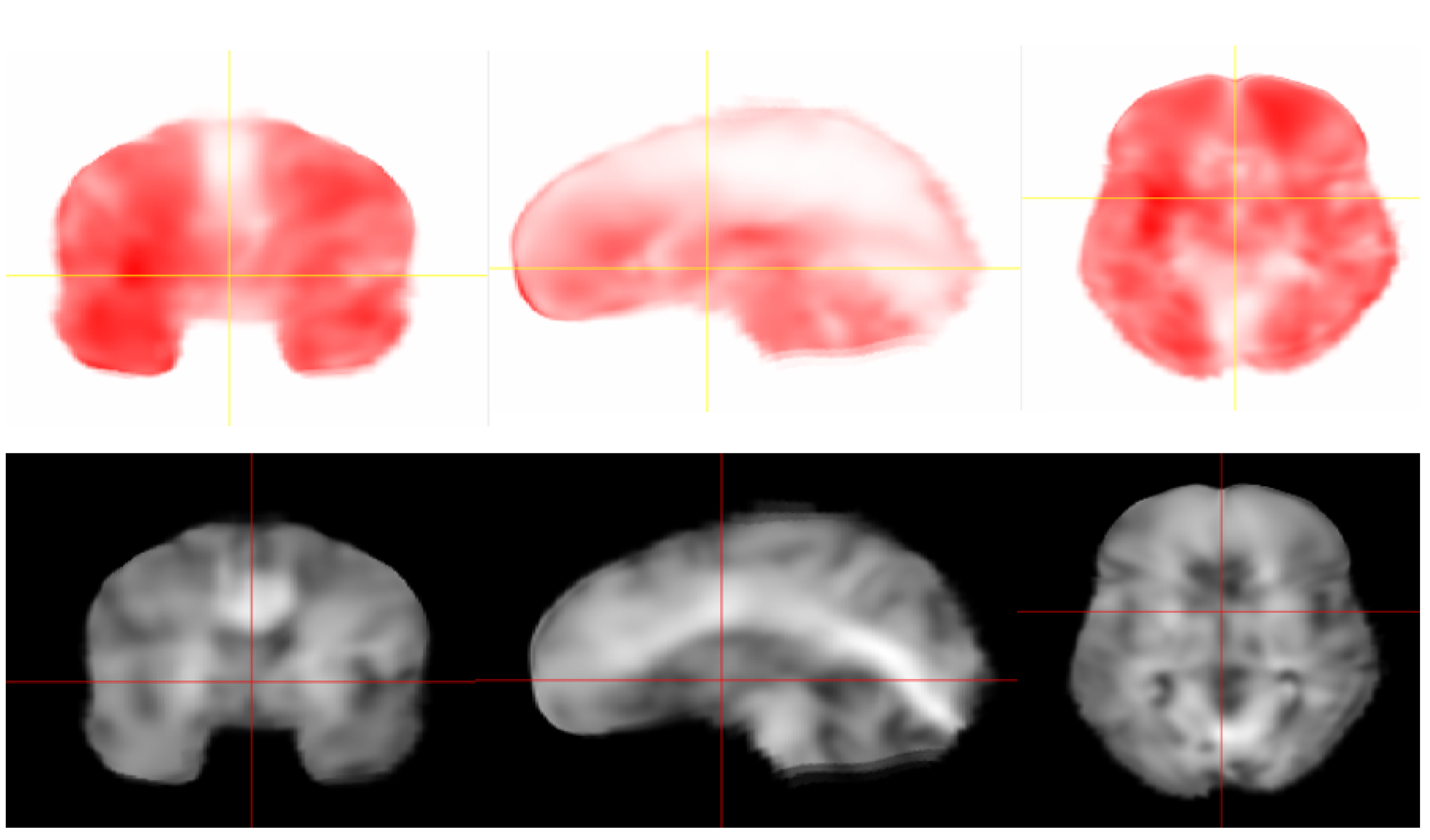
The distribution of storage and loss moduli within the white matter in the imaging resolution (2 × 2 × 2 mm) is presented in Figure 1 for the coronal, sagittal and horizontal planes. The relative stiffness of both the corpus callosum and the corona radiata can be clearly observed. The average values and the standard deviation for the global white and gray matter is presented in Table 1 as well as those for the corpus callosum and corona radiata.
2.2. Finite Element Mesh Generation
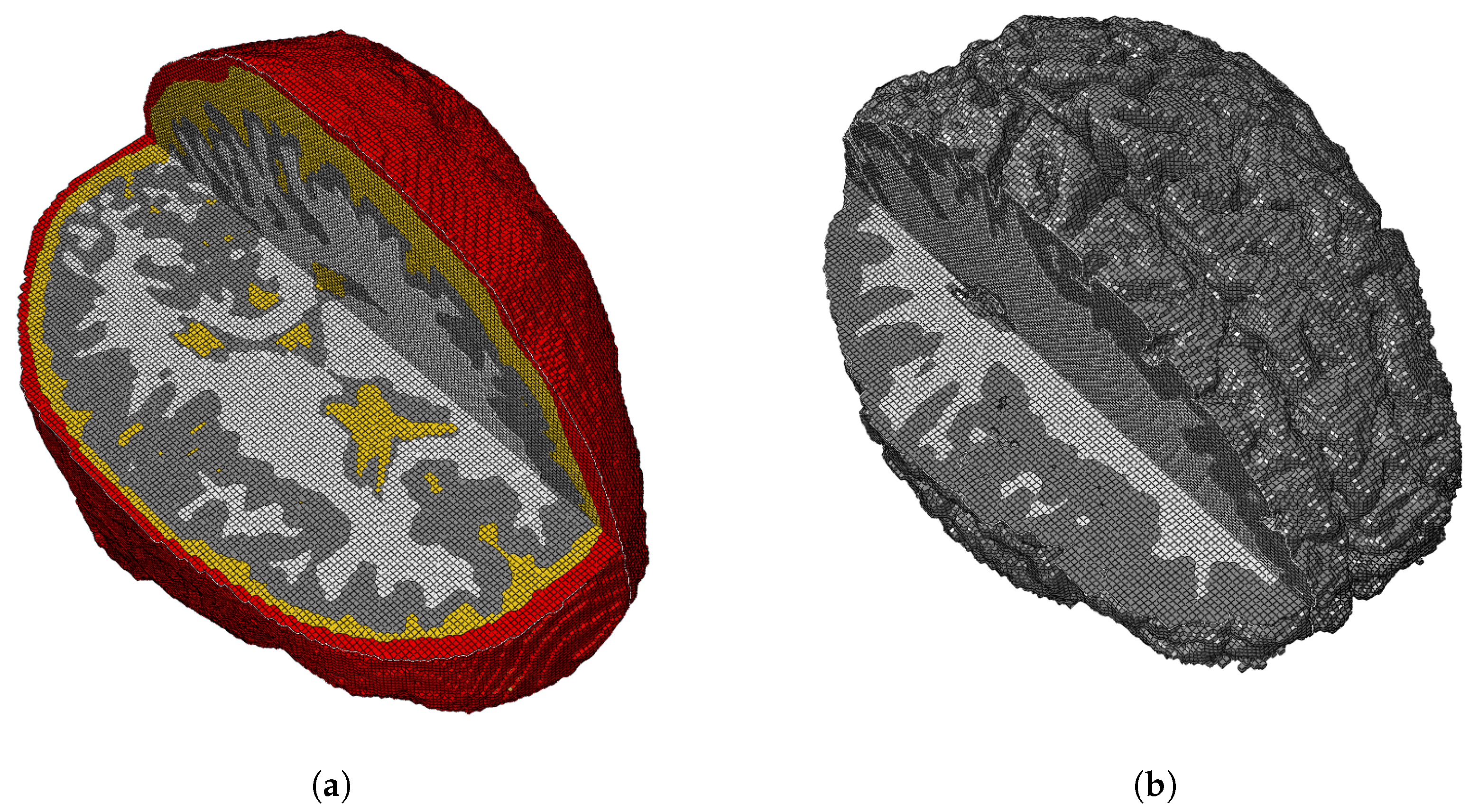
In addition to the MRE image acquisition, T1-weighted anatomical images with a resolution of mm are generated for the purposes of mesh segmentation. Image voxels are directly converted to eight-noded hexahedral elements through a custom code, thus preserving the same spatial resolution as the MRI scans. The resulting mesh consists of approximately 2.2 million elements. The mesh is segmented into the following tissue types: scalp, skull, cerebrospinal fluid (CSF), gray matter and white matter, as depicted in Figure 2. Details of the segmentation can be found in [10]. Each element is assigned a different material definition based on the results of the segmentation, as detailed in Section 2.3. Features that are below the imaging resolution such as membranes, blood vessels, bridging veins, and draining sinuses are excluded from the model. Since T2-weighted scans are not collected, the segmentation of the interfaces between tissue types is negatively affected. We perform a mesh smoothing operation at these interfaces to minimize this effect. We utilize a volume-preserving Laplacian smoothing algorithm, as outlined in [17]. Smoothing has the added benefit of eliminating numerical artifacts that may manifest from jagged edges along interfaces. Reduced integration is used to improve the accuracy of the computed strains as well as to reduce the cost of integration. The integral viscoelastic form of hourglass control is used to suppress hourglass modes.
Our MRI voxel-based approach produces meshes, which realistically model the complicated folding structure of the cerebral cortex (i.e., gyri and sulci) as well as the differentiation of gray and white matter of brain tissues. Additionally, in order to accurately resolve the shear wave motion within the brain, the mesh must be sufficiently refined [8]. For example, using the typical speeds of shear wave propagation in brain tissue, m/s, and the frequency of the vibration as 50 Hz, we arrive at a minimum element size of 10mm (using a conservative choice of 10 elements per wavelength [23]). For vibrations of higher frequency or more transient loading (such as the cases for impact loads), this requirement is even more stringent according to with .
2.3. Material Properties
As discussed above, we assign different material definitions to each voxel based on the result of the mesh segmentation. Due to the presence of highly oriented tracts of myelin-sheathed axonal fibers in white matter, significant heterogeneity exist in this region, especially within the corpus callosum (CC) and corona radiata (CR). On the other hand, gray matter is made up of cell bodies and supporting vascular networks that can be assumed to be isotropic and homogeneous [10,24]. This assumption allows for the MRE imaging to be performed over a manageable acquisition volume. As such, we allow for only the white matter to have material heterogeneity whereas other tissues are assumed to be homogeneous.
For homogeneous tissues, the choice of material properties is determined from data used commonly in the literature, presented in Table 2. The skull is assumed to be linear elastic and modeled as a single-layer structure with homogenized properties given in [25]. For the material model for the CSF, we have the choice of three models, previously presented in [19]: incompressible elastic, viscoelastic, and fluid-like elastic using an equation of the state model. We determined that the choice of CSF affects the shear wave propagation within the brain while the peak pressure is not significantly altered. For the first iteration of our heterogeneous model, we choose the most commonly utilized model—nearly incompressible elastic model with bulk modulus—to be very large compared to the shear modulus, with values taken from [26].
We choose the Ogden hyperelastic material model to accurately capture behavior of brain tissue under large deformations. Additionally, brain tissues are considerably softer in extension than in compression [27]—behavior that a nonlinear model would correctly capture. Research has found that compared to other nonlinear models such as the neo-Hookean or Mooney–Rivlin—the Ogden model performs the best over multiple loading conditions [26,28].
The strain energy functional is a function of the principal strain invariants () of the right Cauchy–Green deformation tensor expressed as:
where and are the Ogden constants; J is the relative volume and K is the bulk modulus. The long-term second Piola–Kirchhoff stress tensor is derived by:
where is the Green strain tensor.
The rate dependence of brain tissue is modeled through a convolution integral:
where the relaxation function, is represented with an N term Prony series of the form:
Here, are the shear relaxation moduli, and are the decay constants.
A second-order Ogden model is used to model the tissues of white and gray matter, with material constants taken from Kleiven [29]. In that work, Kleiven presents a range of material properties fit to the experimental data from [30] using the iterative least-squares method. This is presented as the Average model in Table 3. Two additional models are generated by scaling the values of stiffness parameters and ; while the decay constants, and Ogden parameters are not altered. These models, designated Compliant and Stiff, are one-half and twice as stiff as the Average model, respectively. Using the relationship we arrive at a effective long-term shear modulus of roughly for the Compliant model.
Due to limitations in the MRE inversion, we are limited to a locally linear viscoelastic model (c.f., Equation (2)) for the heterogeneous input data. We therefore incorporate the relative stiffness from MRE and scale the nonlinear material parameters between the three material models presented in Table 3. For each white matter voxel, effective stiffness from MRE inversion is used to scale the hyper-viscoelastic material properties between the extreme Compliant and Stiff models. For the gray matter voxels, the stiffness is chosen to be homogeneous, with values scaled to the average stiffness presented in Table 3. The mass density, decay constants and Ogden parameter are maintained to be homogeneous in all voxels.
2.4. Interface and Boundary Conditions
We ensure traction and displacement continuity at material interfaces, ensuring neither tangential sliding nor separation occurs at any two-tissue interface. We consider two extreme assumptions for the head-neck junction, free and fixed boundary conditions mostly following previous work in [17]. This gives us two extreme cases to recreate the imprecise boundary conditions used in experiments. The free boundary condition allows for predominantly rectilinear motion under frontal impacts while rotational motion cannot be represented. We consider the fixed boundary condition as the other extreme case where the nodes around an area of the foramen magnum are fully constrained. Research reported in [17] showed that the responses from these two boundary conditions bound the experimental response.
2.5. Experimental Verification
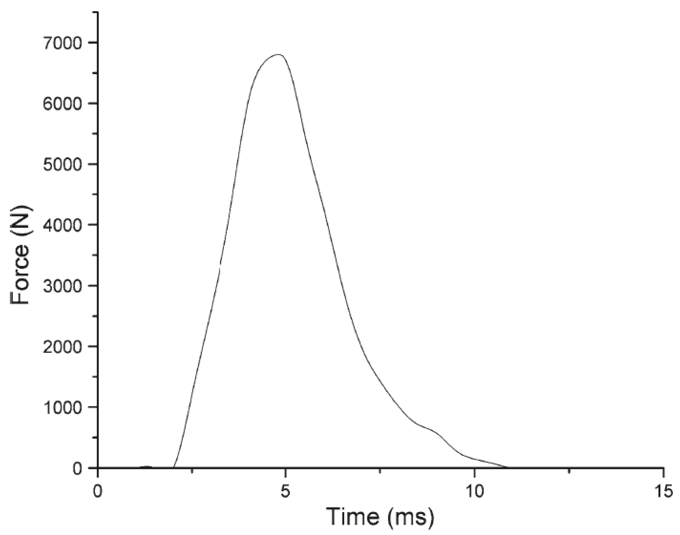
We use Nahum et al. linear impact experiments [31] to verify the accuracy of our model. In the typical experiment, a cylindrical impactor was launched at a seated cadaver at a constant velocity of m/s. The impact was along the specimen’s mid-sagittal plane in an anterior-posterior direction. The skull was rotated such that the Frankfort anatomical plane was inclined to the horizontal. The input force lasts approximately 9 ms, reaching a peak of 6.8 kN, as showed in Figure 3. Intracranial pressure history is recorded during the simulated impact event. The results of this comparison are presented in the next section under both the free and fixed boundary conditions. Our homogeneous model is also verified using tagged MRI and harmonic phase (HARP) imaging analysis techniques in [18], where displacement time history from head-drop experiments is compared to numerical results. Finally, we directly compare displacement data during impact utilizing experimental data from Hardy et al.’s brain translational motion experiment [32,33]. Brain motion is captured using neutral density targets (NDT) under linear accelerations ranging from 38 to 291 g. We use the free boundary conditions to simulate the impact under Hardy’s experiment.
3. Results and Discussion
3.1. Simulation of Impact
The recorded impact force from the frontal cadaveric impact experiment conducted by Nahum, as discussed in the preceding section, is directly applied to the model in the form of a distributed load with the peak pressure input of 4.37 MPa on the frontal region of the skull. The impact pulse lasts about 9 ms and the simulation is run for 15 ms. Rotation of the model is permitted as the base of the skull is not constrained. We find that this free boundary condition gives better correlation of coup pressure to experimental results [17] than the fixed boundary condition. The FE simulations are carried out using Abaqus/Explicit.
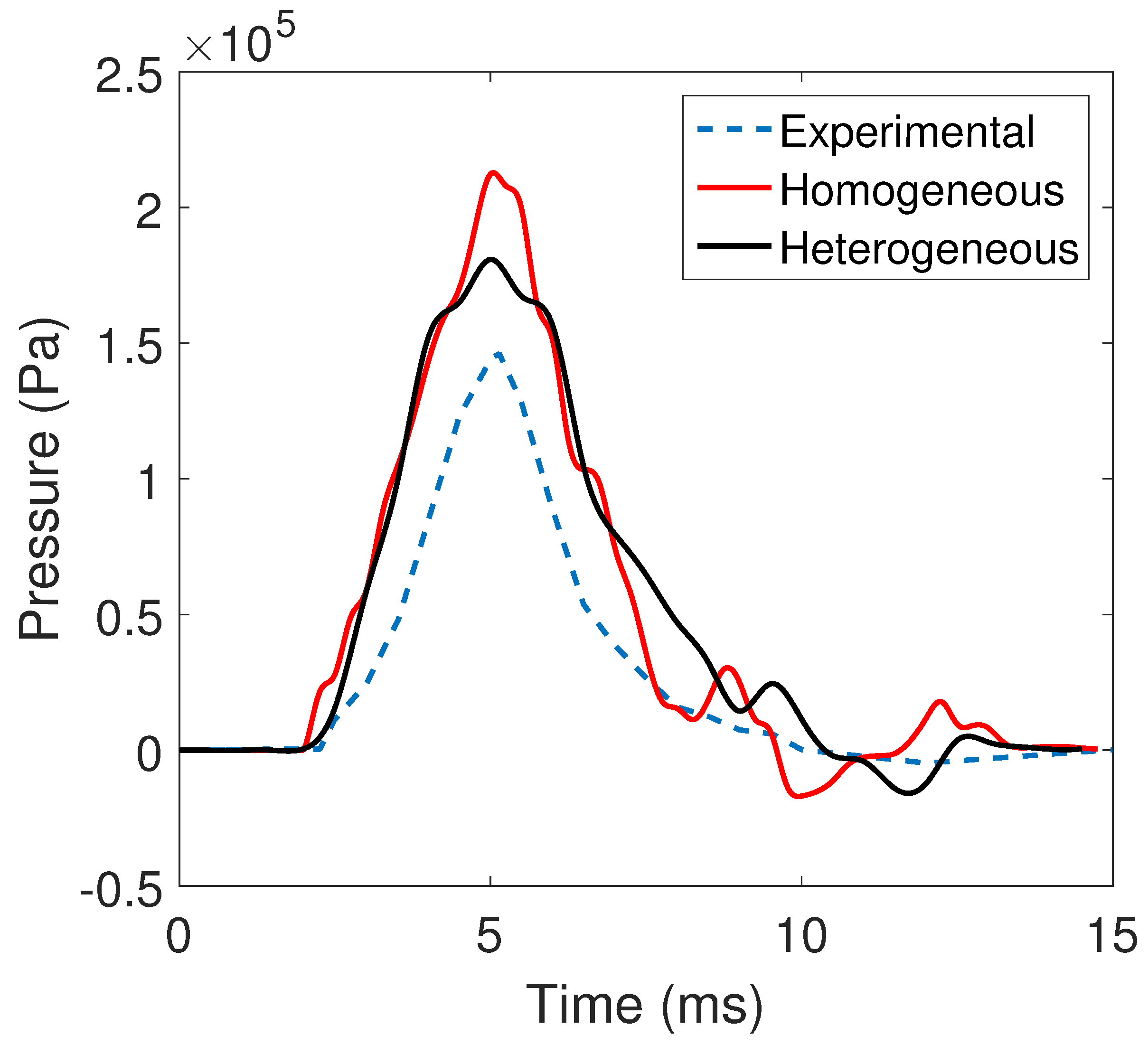
The pressure–time history for the Nahum loading is presented in Figure 4 at the coup impact site. We plot the results for both the homogeneous and heterogeneous models. The model predicts tensile pressure for nearly the whole duration of impact. The peak pressure predicted by the heterogeneous material model more closely matches that from Nahum’s experiments than the homogeneous model. In both cases the peak pressure occurs roughly at the same time, indicating very similar wave speeds.
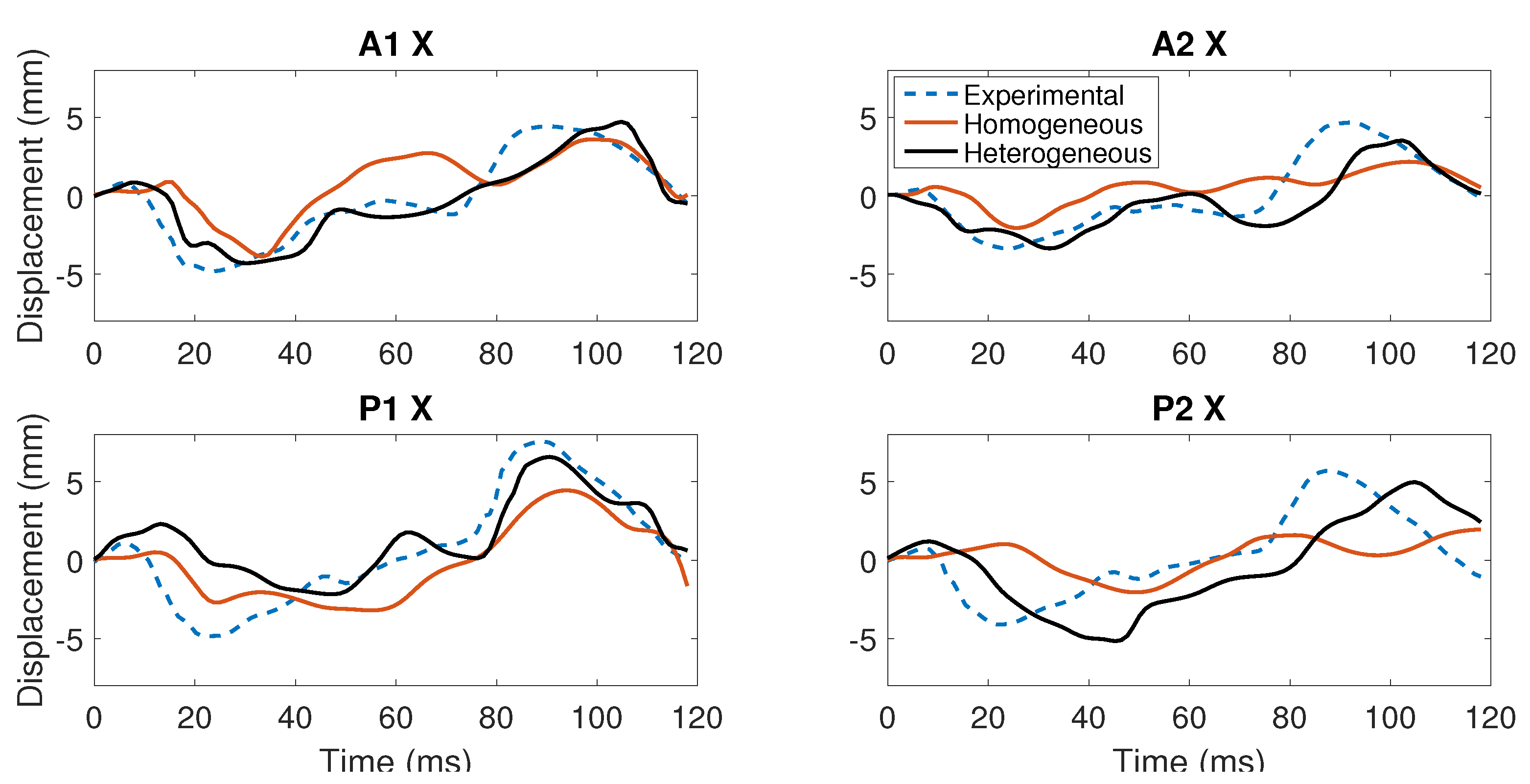
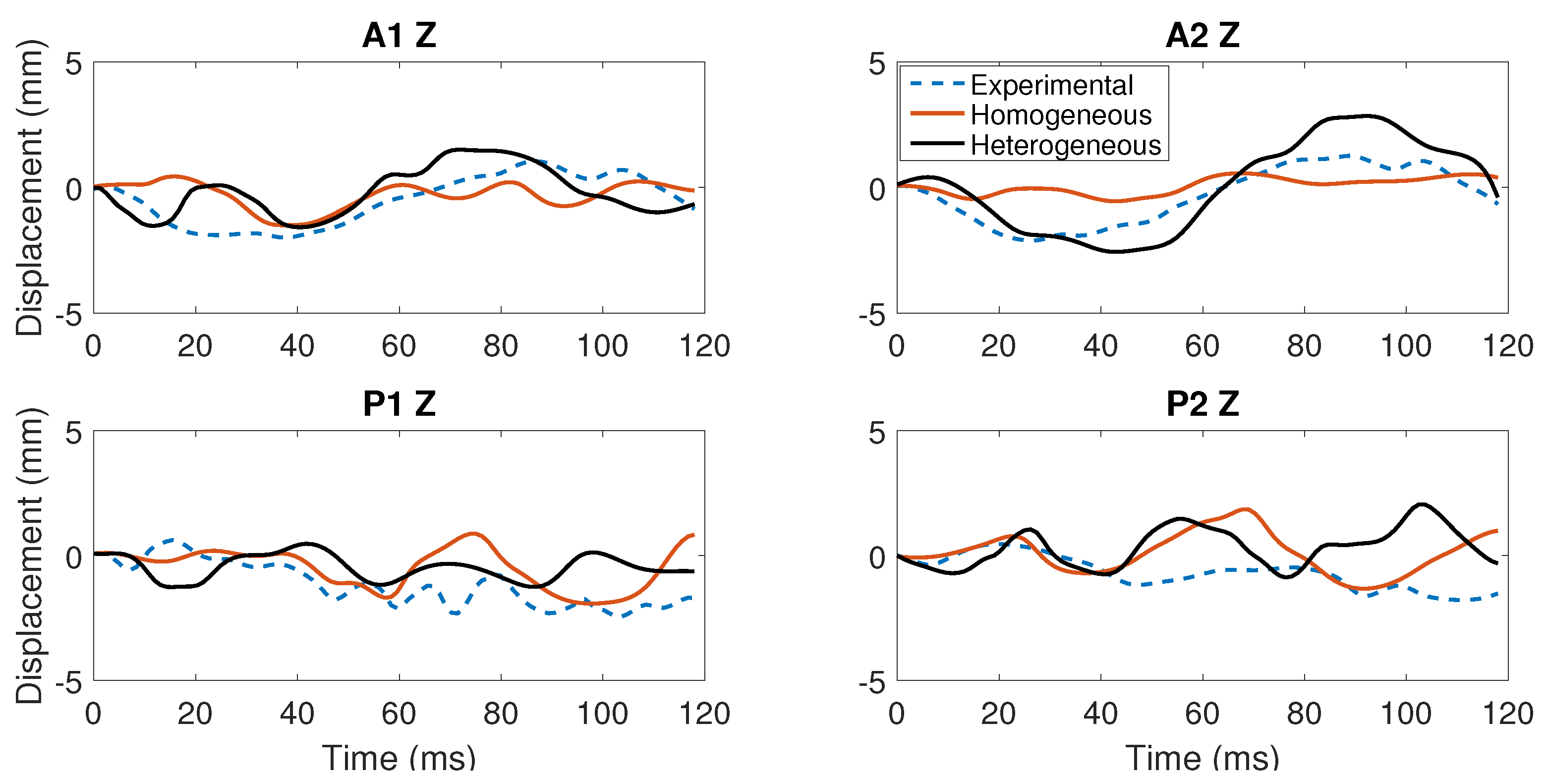
We next compare the displacement response to the C383-T1 impact from Hardy et al. experiments [32]. This is a frontal impact experiment lasting 118 s with displacements captured by two columns of six NDTs. We plot the response for relative displacements for the and directions for two NDTs each in the anterior (A) and posterior (P) positions (labeled A1, A2 and P1, P2, respectively); see Figure 5 and Figure 6. To quantitatively compare the response of the two models, we follow a similar argument as in [26] and compute the displacement magnitude (excursion) at the NDTs. Since injury criteria are based on the magnitude of tissue strain, it is argued that the extension rather than the entire NDT trajectory is more important. We find that the heterogeneous model more consistently and closely predicts the excursion determined experimentally, as presented in Table 4. Additionally, we have previously validated our homogeneous model using tagged MRI and HARP imaging analysis techniques in [18], which allows comparisons of displacement fields for the entire cerebrum in vivo.
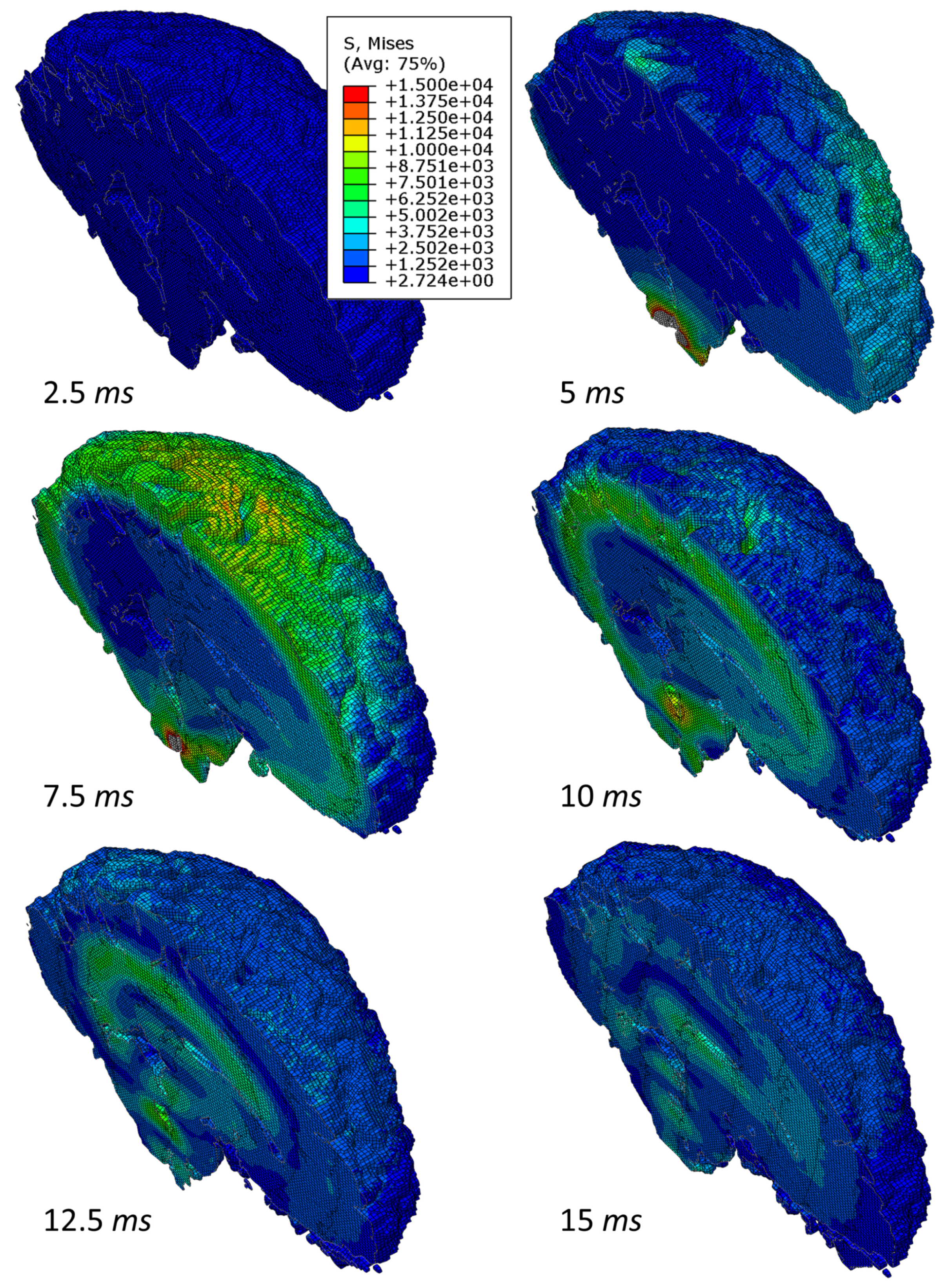
We plot the contours of the von Mises stress distribution on the sagittal plane due to the frontal impact in Figure 7 (also see supplementary simulation video available online). The spherically convergent structure of the shear wave, just like the one found using the linear elastic model of brain’s gray and white matters [17], is clearly observed. The wave attenuates as it travels inwards and eventually dissipates. Reflections of wave due to scattering from heterogeneous white matter structures can also be observed at later times.
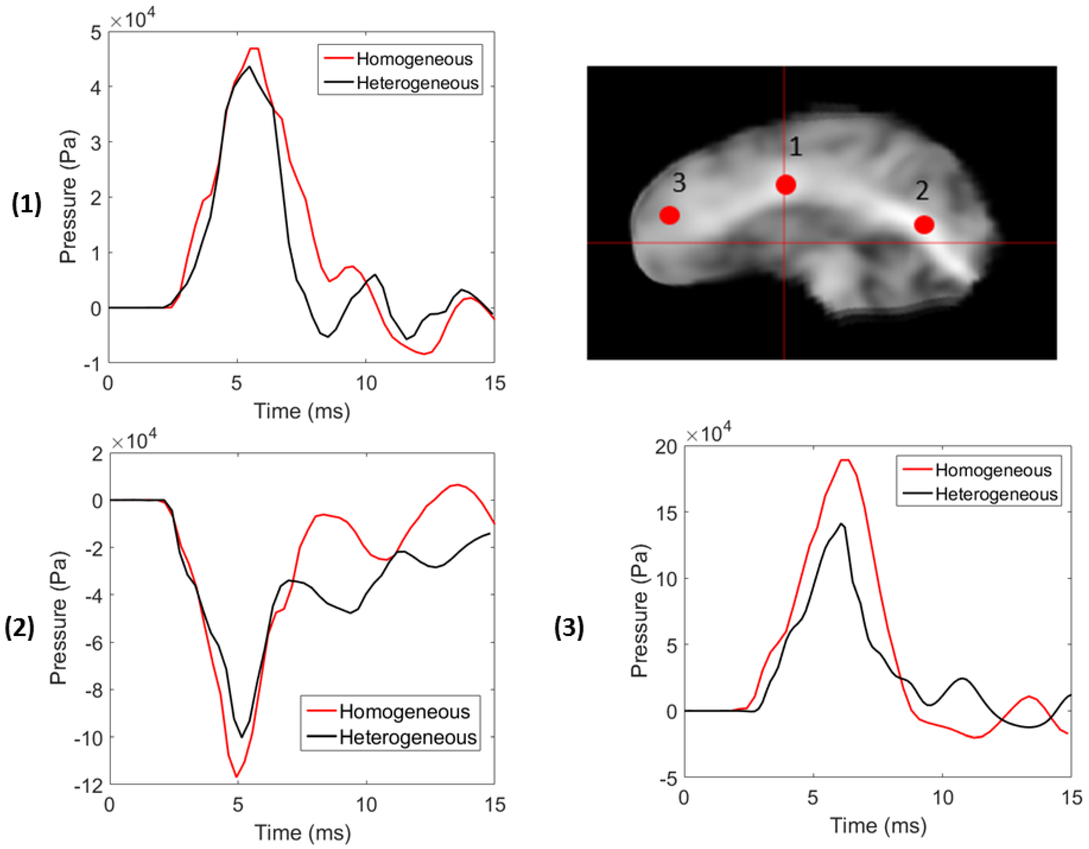
Next, we consider three distinct points along the sagittal plane, as depicted in Figure 8. The points are chosen within regions of strong heterogenities due to the presence of highly aligned axon tracts, such as the corpus callosum and corona radiata. The differences in mechanical properties of these regions are given in Table 5. We see that the material phases at these points are relatively stiffer than the corresponding points in the homogeneous model. As a result, the response in Figure 8 is affected accordingly. We find that the difference in peak pressure response is proportional to the difference in shear stiffness between the homogeneous and heterogeneous models. However, the time at which these events occur is not significantly affected. This indicates that the pressures in regions of high stiffness within the brain are over-estimated in the homogeneous models. In summary, relative to the MRI-based model, the new MRE-based heterogeneous model more accurately predicts the local response within the white matter by taking into account the differences in tissue stiffness of local white matter structures.
A few points are in order regarding the qualitative differences between the shear modulus of different regions in our model. Globally, the white matter is found to be approximately stiffer than the gray matter. In general, the white matter properties in local regions differ significantly from the average ones. For instance, the storage modulus is significantly lower in the rest of the white matter than within the corpus callosum and the corona radiata [10]. This is quite logical given the fact that the corpus callosum contains highly oriented, tightly packed axon tracts. The corpus callosum, in fact, is stiffer than the corona radiata, again evident from the composition of the corona radiata, which contains axon fibers that fan out and are not as highly aligned as the corpus callosum. Indeed, experiments have found that the fractional anisotropty (FA) values for the corpus callosum and corona radiata are in the range of 0.6–1.0 and 0.4–0.6, respectively [34,35].
Additionally, while both white and gray matter have similar values of damping ratio, (which reflects the amount of motion attenuation within the tissue), the corpus callosum has a lower value while the corona radiata has a higher value. This can be explained by examining the microstructure of each of these regions. Experiments by Guo et al. [36] demonstrated that the damping ratio (and thus, the attenuation) in soft tissue composites increases as the number of cross-links between fibers increases. The corona radiata consists of fibers arranged in a grid-like pattern [37] with a large number of cross-links. These crossings do not exist in the corpus callosum, offering a possible explanation for the distribution of .
Since mechanical measures from MRE and diffusivity measures from diffuse tensor imaging (DTI) both provide insight into the heterogeneity within the white matter, a natural question arises here: What is the difference between our heterogeneous (yet isotropic) model and the more common anisotropic FE models where fiber anisotropy is determined from DTI scans? Many such examples of the latter exist in the literature: for instance in [38,39,40,41]. Johnson et al. [10] performed both MRE and DTI measurements on a group of seven volunteers to determine the correlation of mechanical and diffusivity measures within the corpus callosum and corona radiata. They determined that MRE and DTI measures correlate well with each other within the corpus callosum—not surprising since they are both sensitive to the underlying tissue microstructure. They hypothesize that these measures are highly dependent on axon diameter since larger axons provide greater structural rigidity to the tissue [42]. Within the corona radiata, however, the correlation is not as significant. The corona radiata comprises fiber tracts that fan towards the cortex and contain numerous crossings [37] which are not captured well by DTI [43]. This has been hypothesized as the reason for the poor correlation within the corona radiata. More work is needed to determine the differences between these two methods when used within FE models.
3.2. Stochastic Wave Propagation
The highly heterogeneous structure of the brain tissue introduces wave scattering that competes with wave amplification due to spherically convergent implosion. Following the development in [44], we investigate this effect by considering the theory of wavefronts. For the case of one-dimensional wave motion, we assume that a compressive load produces a shock wavefront that propagates from a disturbed domain to an undisturbed one with a speed . The initial conditions can be given as where H is the Heaviside function.
Assuming a plane wave in a homogeneous medium, we have the dynamic compatibility condition in the -plane, where denotes the discontinuity in a function across the boundary of two materials, is the shear stress, is the mass density, u is the displacement normal to the direction of wave motion, and is the transverse wave speed. The linear viscoelastic stress–strain relation for a process that started at time is
where is the shear strain. We can derive the relationship for the wave speed as , where is the glassy modulus. Following the derivation in [44], we obtain the equation governing the evolution of the discontinuity of at the wavefront as:
On account of the initial conditions above, the solution of Equation (10) is
Given that and , the stress jump exhibits exponential attenuation and has a tendency for blow-up as . As our simulations here and in [19] demonstrate, the attenuation is sufficiently strong so that the imploding waves generated from transient impacts do not blow up into a singularity at the head center.
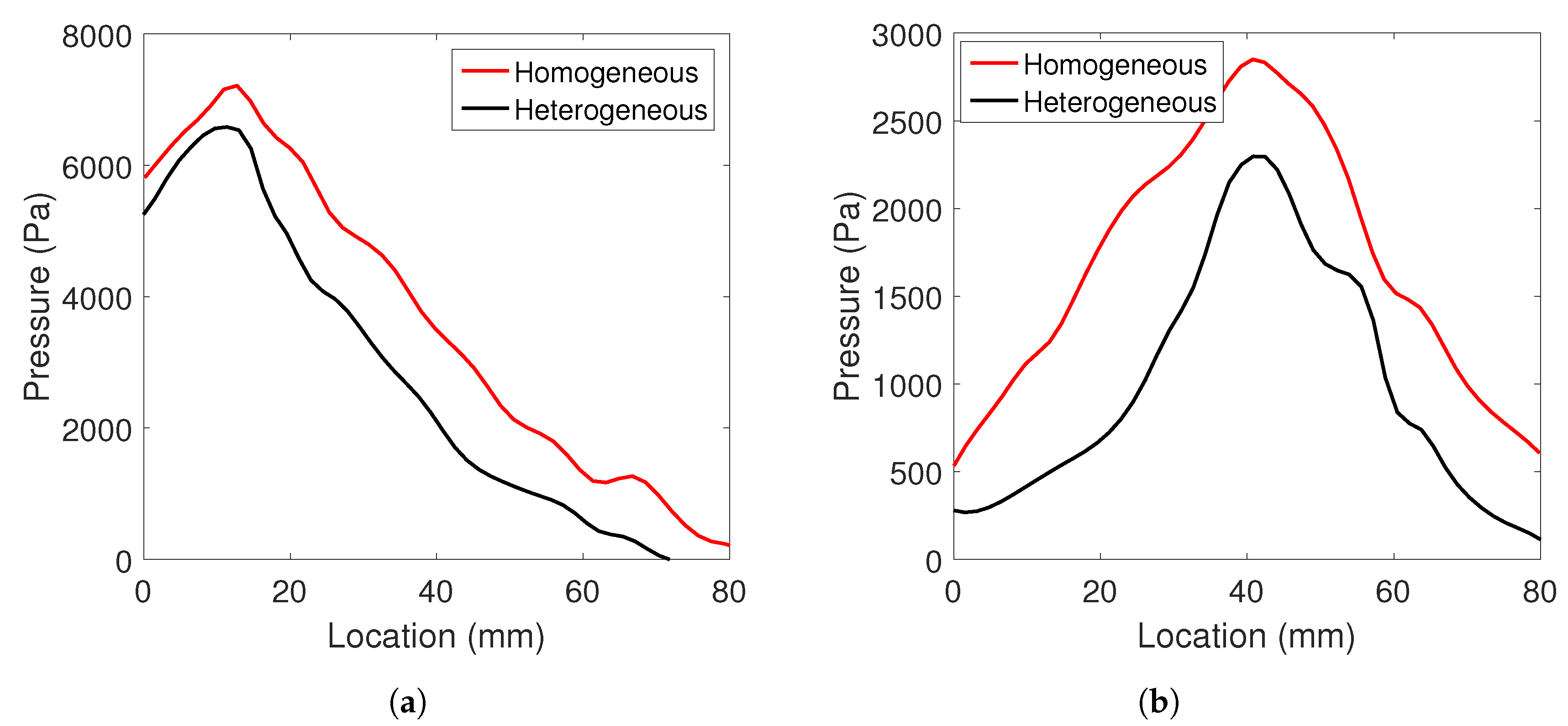
The impact results not only in a fast pressure wave, but also in a slower shear wave. Due to its relatively low shear modulus, brain tissue deforms much more easily in shear than in dilatation mode. Thus, the shear wave is potentially more damaging. Recall that the spherically convergent shear wave patterns are observed even in the case of homogeneous material description, c.f. [17]. The attenuations of pressure along the sagittal plane for both the homogeneous and heterogeneous models are presented in Figure 9. It is clear that the attenuation is greater in the heterogeneous model as predicted. This is consistent with studies of transient wave propagation in elastodynamics of random media [45,46].
3.3. Limitations
This section discusses a few limitations of our methodology, some of which are likely to be improved in future works. First, features that are below the imaging resolution such as membranes (in particular, the falx cerebri and tentorium), bridging veins and blood vessels are excluded from the current model. However, we argue that the inclusion of heterogeneous MRE-derived parameters in white matter tissue alleviates some of the drawbacks of excluding these features. Additionally, since the MRE inversion is performed assuming a locally linear viscoelastic material model, we are limited to include only relative stiffness from MRE and not the absolute moduli measured. A limitation of MRE is that displacement is induced in the small strain regime. While our current model is able to accurately capture experimental response, it has not been validated for large deformations yet.
4. Conclusions
Our high resolution, hyper-viscoelastic FE head model now includes heterogeneities of white matter structures improving the ability to capture wave dynamics during highly transient impact events. Heterogeneous shear modulus is determined using a nonlinear inversion technique from MRE experiments performed by [10]. While many FE models employ homogenized or averaged mechanical properties to approximate constitutive relations of brain tissues, our approach allows us to investigate response due to local structures within the white matter. Previous experiments have shown that both the corpus callosum and corona radiata are significantly stiffer than overall white matter, with the corpus callosum exhibiting greater stiffness and less viscous damping than the corona radiata. These differences are explained by examining the organizational and compositional characteristics of each structure. Incorporating this heterogeneity in our model affects wave propagation within the cerebrum and yields results that more closely match experimental results. We find that local variations in stiffness affect the local mechanical response; for instance, intracranial pressure magnitude following an impact is lower in regions of high local stiffness. Finally, shear wave attenuation is observed to be more pronounced in the heterogeneous material model and this aspect introduces extra shear wave scattering in addition to the damping effect of tissue viscoelasticity.
Supplementary Materials
The following are available online at https://0-www-mdpi-com.brum.beds.ac.uk/2673-3951/1/2/14/s1.
Author Contributions
Both authors conceived of and designed the study. A.M. has carried out all the research, made all the figures, and drafted the manuscript, except for Section 3.2. All authors have read and agreed to the published version of the manuscript.
Funding
This research received no external funding.
Acknowledgments
The authors thank the anonymous reviewers and Karol Miller for their stimulating comments and valuable suggestions that greatly improved this paper. In addition, we thank Curtis Johnson and Bradley Sutton for providing the MRE data sets used in the model.
Conflicts of Interest
The authors declare no conflict of interest.
References
- Taylor, C.A.; Bell, J.M.; Breiding, M.J.; Xu, L. Traumatic Brain Injury-Related Emergency Department Visits, Hospitalizations, and Deaths-United States, 2007 and 2013. MMWR Surveill Summ. 2017, 66, 1–16. [Google Scholar] [CrossRef]
- Gennarelli, T.A.; Thibault, L.E.; Adams, J.H.; Graham, D.I.; Thompson, C.J.; Marcincin, R.P. Diffuse axonal injury and traumatic coma in the primate. Ann. Neurol. 1982, 12, 564–574. [Google Scholar] [CrossRef]
- Gentry, L.R.; Godersky, J.C.; Thompson, B.; Dunn, V.D. Prospective comparative study of intermediate-field MR and CT in the evaluation of closed head trauma. Am. J. Roentgenol. 1988, 150, 673–682. [Google Scholar] [CrossRef] [PubMed] [Green Version]
- Gentry, L.R.; Godersky, J.C.; Thompson, B. MR imaging of head trauma: Review of the distribution and radiopathologic features of traumatic lesions. Am. J. Roentgenol. 1988, 150, 663–672. [Google Scholar] [CrossRef] [PubMed] [Green Version]
- Ng, H.; Mahaliyana, R.; Poon, W. The pathological spectrum of diffuse axonal injury in blunt head trauma: assessment with axon and myelin stains. Clin. Neurol. Neurosurg. 1994, 96, 24–31. [Google Scholar] [CrossRef]
- Arfanakis, K.; Haughton, V.M.; Carew, J.D.; Rogers, B.P.; Dempsey, R.J.; Meyerand, M.E. Diffusion tensor MR imaging in diffuse axonal injury. Am. J. Neuroradiol. 2002, 23, 794–802. [Google Scholar]
- Arbogast, K.B.; Margulies, S.S. Material characterization of the brainstem from oscillatory shear tests. J. Biomech. 1998, 31, 801–807. [Google Scholar] [CrossRef]
- Madhukar, A.; Ostoja-Starzewski, M. Finite element methods in human head impact simulations: A review. Ann. Biomed. Eng. 2019, 47, 1832–1854. [Google Scholar] [CrossRef]
- Chatelin, S.; Constantinesco, A.; Willinger, R. Fifty years of brain tissue mechanical testing: From in vitro to in vivo investigations. Biorheology 2010, 47, 255–276. [Google Scholar] [CrossRef]
- Johnson, C.L.; McGarry, M.D.; Gharibans, A.A.; Weaver, J.B.; Paulsen, K.D.; Wang, H.; Olivero, W.C.; Sutton, B.P.; Georgiadis, J.G. Local mechanical properties of white matter structures in the human brain. Neuroimage 2013, 79, 145–152. [Google Scholar] [CrossRef] [Green Version]
- Muthupillai, R.; Lomas, D.; Rossman, P.; Greenleaf, J.F.; Manduca, A.; Ehman, R.L. Magnetic resonance elastography by direct visualization of propagating acoustic strain waves. Science 1995, 269, 1854–1857. [Google Scholar] [CrossRef] [PubMed]
- Sack, I.; Streitberger, K.J.; Krefting, D.; Paul, F.; Braun, J. The influence of physiological aging and atrophy on brain viscoelastic properties in humans. PLoS ONE 2011, 6, e23451. [Google Scholar] [CrossRef] [PubMed]
- Murphy, M.C.; Huston, J., III; Jack, C.R., Jr.; Glaser, K.J.; Manduca, A.; Felmlee, J.P.; Ehman, R.L. Decreased brain stiffness in Alzheimer’s disease determined by magnetic resonance elastography. J. Magn. Reson. Imaging 2011, 34, 494–498. [Google Scholar] [CrossRef] [PubMed] [Green Version]
- Murphy, M.C.; Huston, J.; Glaser, K.J.; Manduca, A.; Meyer, F.B.; Lanzino, G.; Morris, J.M.; Felmlee, J.P.; Ehman, R.L. Preoperative assessment of meningioma stiffness using magnetic resonance elastography. J. Neurosurg. 2013, 118, 643–648. [Google Scholar] [CrossRef]
- Boulet, T.; Kelso, M.L.; Othman, S.F. Microscopic magnetic resonance elastography of traumatic brain injury model. J. Neurosci. Methods 2011, 201, 296–306. [Google Scholar] [CrossRef]
- Van Houten, E.E.; Miga, M.I.; Weaver, J.B.; Kennedy, F.E.; Paulsen, K.D. Three-dimensional subzone-based reconstruction algorithm for MR elastography. Magn. Reson. Med. 2001, 45, 827–837. [Google Scholar] [CrossRef]
- Chen, Y.; Ostoja-Starzewski, M. MRI-based finite element modeling of head trauma: Spherically focusing shear waves. Acta Mech. 2010, 213, 155–167. [Google Scholar] [CrossRef]
- Chen, Y.; Sutton, B.; Conway, C.; Broglio, S.P.; Ostoja-Starzewski, M. Brain Deformation Under Mild Impact: Magnetic Resonance Imaging-Based Assessment and Finite Elmenent Study. Int. J. Numer. Anal. Model. Ser. B 2012, 3, 20–35. [Google Scholar]
- Madhukar, A.; Chen, Y.; Ostoja-Starzewski, M. Effect of cerebrospinal fluid modeling on spherically convergent shear waves during blunt head trauma. Int. J. Numer. Methods Biomed. Eng. 2017, 33. [Google Scholar] [CrossRef]
- Johnson, C.L.; McGarry, M.D.J.; Van Houten, E.E.W.; Weaver, J.B.; Paulsen, K.D.; Sutton, B.P.; Georgiadis, J.G. Magnetic resonance elastography of the brain using multishot spiral readouts with self-navigated motion correction. Magn. Reson. Med. 2013, 70, 404–412. [Google Scholar] [CrossRef] [Green Version]
- Glover, G.H. Simple analytic spiral K-space algorithm. Magn. Reson. Med. 1999, 42, 412–415. [Google Scholar] [CrossRef]
- McGarry, M.D.J.; Van Houten, E.E.W. Use of a Rayleigh damping model in elastography. Med. Biol. Eng. Comput. 2008, 46, 759–766. [Google Scholar] [CrossRef] [PubMed]
- Bradshaw, D.; Morfey, C. Pressure and shear response in brain injury models. In Proceedings of the 17th International Technical Conference on the Enhanced Safety of Vehicles, Amsterdam, The Netherlands, 4–7 June 2001. [Google Scholar]
- Prange, M.; Margulies, S. Regional, directional, and age-dependent properties of the brain undergoing large deformation. J. Biomech. Eng. 2002, 124, 244–252. [Google Scholar] [CrossRef] [PubMed] [Green Version]
- Khalil, T.B.; Hubbard, R.P. Parametric study of head response by finite element modeling. J. Biomech. 1977, 10, 119–132. [Google Scholar] [CrossRef]
- Wang, F.; Han, Y.; Wang, B.; Peng, Q.; Huang, X.; Miller, K.; Wittek, A. Prediction of brain deformations and risk of traumatic brain injury due to closed-head impact: Quantitative analysis of the effects of boundary conditions and brain tissue constitutive model. Biomech. Model. Mechanobiol. 2018, 17, 1165–1185. [Google Scholar] [CrossRef] [PubMed]
- Miller, K.; Chinzei, K. Mechanical properties of brain tissue in tension. J. Biomech. 2002, 35, 483–490. [Google Scholar] [CrossRef] [Green Version]
- Budday, S.; Sommer, G.; Birkl, C.; Langkammer, C.; Haybaeck, J.; Kohnert, J.; Bauer, M.; Paulsen, F.; Steinmann, P.; Kuhl, E.; et al. Mechanical characterization of human brain tissue. Acta Biomater. 2017, 48, 319–340. [Google Scholar] [CrossRef]
- Kleiven, S. Predictors for Traumatic Brain Injuries Evaluated through Accident Reconstructions. 2007. Available online: https://0-saemobilus-sae-org.brum.beds.ac.uk/content/2007-22-0003 (accessed on 10 December 2020).
- Franceschini, G.; Bigoni, D.; Regitnig, P.; Holzapfel, G.A. Brain tissue deforms similarly to filled elastomers and follows consolidation theory. J. Mech. Phys. Solids 2006, 54, 2592–2620. [Google Scholar] [CrossRef]
- Nahum, A.M.; Smith, R.; Ward, C.C. Intracranial Pressure Dynamics during Head Impact. 1977. Available online: https://www.sae.org/publications/technical-papers/content/770922/ (accessed on 10 December 2020).
- Hardy, W.N.; Foster, C.D.; Mason, M.J.; Yang, K.H.; King, A.I.; Tashman, S. Investigation of head injury mechanisms using neutral density technology and high-speed biplanar X-ray. Stapp Car Crash J. 2001, 45, 337–368. [Google Scholar]
- Hardy, W.N.; Mason, M.J.; Foster, C.D.; Shah, C.S.; Kopacz, J.M.; Yang, K.H.; King, A.I.; Bishop, J.; Bey, M.; Anderst, W.; et al. A study of the response of the human cadaver head to impact. Stapp Car Crash J. 2007, 51, 17. [Google Scholar]
- Bozzali, M.; Falini, A.; Franceschi, M.; Cercignani, M.; Zuffi, M.; Scotti, G.; Comi, G.; Filippi, M. White matter damage in Alzheimer’s disease assessed in vivo using diffusion tensor magnetic resonance imaging. J. Neurol. Neurosurg. Psychiatry 2002, 72, 742–746. [Google Scholar] [CrossRef] [PubMed] [Green Version]
- Lee, C.E.; Danielian, L.E.; Thomasson, D.; Baker, E.H. Normal regional fractional anisotropy and apparent diffusion coefficient of the brain measured on a 3 T MR scanner. Neuroradiology 2009, 51, 3–9. [Google Scholar] [CrossRef] [PubMed]
- Guo, J.; Posnansky, O.; Hirsch, S.; Scheel, M.; Taupitz, M.; Braun, J.; Sack, I. Fractal network dimension and viscoelastic powerlaw behavior: II. An experimental study of structure-mimicking phantoms by magnetic resonance elastography. Phys. Med. Biol. 2012, 57, 4041. [Google Scholar] [CrossRef] [PubMed]
- Wedeen, V.J.; Rosene, D.L.; Wang, R.; Dai, G.; Mortazavi, F.; Hagmann, P.; Kaas, J.H.; Tseng, W.Y.I. The geometric structure of the brain fiber pathways. Science 2012, 335, 1628–1634. [Google Scholar] [CrossRef] [Green Version]
- Ji, S.; Zhao, W.; Ford, J.C.; Beckwith, J.G.; Bolander, R.P.; Greenwald, R.M.; Flashman, L.A.; Paulsen, K.D.; McAllister, T.W. Group-wise evaluation and comparison of white matter fiber strain and maximum principal strain in sports-related concussion. J. Neurotrauma 2015, 32, 441–454. [Google Scholar] [CrossRef]
- Giordano, C.; Kleiven, S. Connecting fractional anisotropy from medical images with mechanical anisotropy of a hyperviscoelastic fibre-reinforced constitutive model for brain tissue. J. R. Soc. Interface 2014, 11, 20130914. [Google Scholar] [CrossRef]
- Giordano, C.; Cloots, R.; Van Dommelen, J.; Kleiven, S. The influence of anisotropy on brain injury prediction. J. Biomech. 2014, 47, 1052–1059. [Google Scholar] [CrossRef]
- Garimella, H.T.; Kraft, R.H. Modeling the mechanics of axonal fiber tracts using the embedded finite element method. Int. J. Numer. Methods Biomed. Eng. 2017, 33. [Google Scholar] [CrossRef]
- Arbogast, K.B.; Margulies, S.S. A fiber-reinforced composite model of the viscoelastic behavior of the brainstem in shear. J. Biomech. 1999, 32, 865–870. [Google Scholar] [CrossRef]
- Wedeen, V.J.; Hagmann, P.; Tseng, W.Y.I.; Reese, T.G.; Weisskoff, R.M. Mapping complex tissue architecture with diffusion spectrum magnetic resonance imaging. Magn. Reson. Med. 2005, 54, 1377–1386. [Google Scholar] [CrossRef]
- Ostoja-Starzewski, M.; Costa, L. Shock waves in random viscoelastic media. Acta Mech. 2012, 223, 1777–1788. [Google Scholar] [CrossRef]
- Nishawala, V.; Ostoja-Starzewski, M.; Leamy, M.; Porcu, E. Lamb’s problem on random mass density fields with fractal and Hurst effects. Proc. R. Soc. Math. Phys. Eng. Sci. 2016, 472, 20160638. [Google Scholar] [CrossRef] [PubMed]
- Zhang, X.; Ostoja-Starzewski, M. Impact force and moment problems on random mass density fields with fractal and Hurst effects. Philos. Trans. R. Soc. A 2020, 378, 20190591. [Google Scholar] [CrossRef] [PubMed]
Figure 1.
Distribution of Loss (top) and Storage (bottom) modulus in the Finite Element (FE) model. Darker regions indicate higher magnitude of shear modulus.
Figure 1.
Distribution of Loss (top) and Storage (bottom) modulus in the Finite Element (FE) model. Darker regions indicate higher magnitude of shear modulus.

Figure 2.
(a) Voxel-based finite element mesh segmented into skull (red), cerebrospinal fluid (CSF) (yellow), gray matter (gray) and white matter (white). (b) Surface of cerebral cortex with sulci and gyri clearly resolved.
Figure 2.
(a) Voxel-based finite element mesh segmented into skull (red), cerebrospinal fluid (CSF) (yellow), gray matter (gray) and white matter (white). (b) Surface of cerebral cortex with sulci and gyri clearly resolved.

Figure 3.
Input force time history (adapted from [17]).
Figure 3.
Input force time history (adapted from [17]).

Figure 4.
Comparison of heterogeneous model with experimental data from [31]. We find that the heterogeneous model exhibits a response closer to the Nahum et al. [31] data.

Figure 5.
Comparison of displacements in the direction for two positions in the anterior (A) and posterior (P) to the Hardy C383-T1 experiment.
Figure 5.
Comparison of displacements in the direction for two positions in the anterior (A) and posterior (P) to the Hardy C383-T1 experiment.

Figure 6.
Comparison of displacements in the direction for two positions in the anterior (A) and posterior (P) to the Hardy C383-T1 experiment.
Figure 6.
Comparison of displacements in the direction for two positions in the anterior (A) and posterior (P) to the Hardy C383-T1 experiment.

Figure 7.
Shear wave propagation due to frontal impact. Notice the attenuation of the wavefront as time progresses.
Figure 7.
Shear wave propagation due to frontal impact. Notice the attenuation of the wavefront as time progresses.

Figure 8.
Comparison of pressure at three points on the sagittal plane. The difference in the heterogeneous and homogeneous models is most evident in regions of high relative stiffness.
Figure 8.
Comparison of pressure at three points on the sagittal plane. The difference in the heterogeneous and homogeneous models is most evident in regions of high relative stiffness.

Figure 9.
Comparison of attenuation of pressure wave along the sagittal plane between homogeneous and heterogeneous model. (a) At 3 ms and (b) at 7 ms.
Figure 9.
Comparison of attenuation of pressure wave along the sagittal plane between homogeneous and heterogeneous model. (a) At 3 ms and (b) at 7 ms.


Table 1.
Average values and standard deviations for different tissues within the model: Gray Matter (GM), White Matter (WM), Corpus Callosum (CC), Corona Radiata (CR).
Table 1.
Average values and standard deviations for different tissues within the model: Gray Matter (GM), White Matter (WM), Corpus Callosum (CC), Corona Radiata (CR).
| GM | WM | CC | CR | |
|---|---|---|---|---|
| G (kPa) | ||||
| G (kPa) | ||||
Table 2.
Material properties of different tissues used in the FE model.
| Tissue | Mass Density (kg/m) | Bulk Modulus K (Pa) | Shear Modulus G (Pa) |
|---|---|---|---|
| Skull [25] | 2070 | 3.61 × | 2.7 × |
| Grey Matter | 1040 | Hyperviscoelastic | |
| White Matter | 1040 | Hyperviscoelastic | |
| Mass Density (kg/m) | Young’s Modulus E (Pa) | Poisson Ratio | |
| CSF [26] | 1000 | 160 | 0.49 |
Table 3.
Hyper-viscoelastic material properties [29].
Table 3.
Hyper-viscoelastic material properties [29].
| ‘Compliant’ | ‘Average’ | ‘Stiff’ | |
|---|---|---|---|
| (Pa) | 26.9 | 53.8 | 107.6 |
| (Pa) | −60.2 | −120.4 | −240.8 |
| 10.1 | 10.1 | 10.1 | |
| −12.9 | −12.9 | −12.9 | |
| 160 | 320 | 640 | |
| 39 | 78 | 156 | |
| 3.1 | 6.2 | 12.4 | |
| 4.0 | 8.0 | 16.0 | |
| 0.05 | 0.10 | 0.20 | |
| 1.5 | 3.0 | 6.0 | |
| ⋮ | ⋮ | ⋮ | ⋮ |
Table 4.
Total excursions (in mm) for Hardy’s C383-T1 experiment compared to the predicted values for two models.
Table 4.
Total excursions (in mm) for Hardy’s C383-T1 experiment compared to the predicted values for two models.
| Location | Experiment | Homogeneous | Heterogeneous |
|---|---|---|---|
| A1 | 9.24 | 7.47 | 9.02 |
| A2 | 8.04 | 4.22 | 6.88 |
| P1 | 12.42 | 7.66 | 8.76 |
| P2 | 9.80 | 4.01 | 10.14 |
Table 5.
Difference of material properties and peak pressure, displacement response for three distinct points (indicated in Figure 8) along the sagittal plane within the white matter.
Table 5.
Difference of material properties and peak pressure, displacement response for three distinct points (indicated in Figure 8) along the sagittal plane within the white matter.
| Location | % Difference in Shear Modulus () | % Difference in Peak Pressure | % Difference in Peak Displacement |
|---|---|---|---|
| 1 | 12.11 | −9.12 | −3.16 |
| 2 | 24.75 | −13.91 | −6.62 |
| 3 | 18.67 | −29.05 | −12.96 |
Publisher’s Note: MDPI stays neutral with regard to jurisdictional claims in published maps and institutional affiliations. |
© 2020 by the authors. Licensee MDPI, Basel, Switzerland. This article is an open access article distributed under the terms and conditions of the Creative Commons Attribution (CC BY) license (http://creativecommons.org/licenses/by/4.0/).
Share and Cite
MDPI and ACS Style
Madhukar, A.; Ostoja-Starzewski, M. Modeling and Simulation of Head Trauma Utilizing White Matter Properties from Magnetic Resonance Elastography. Modelling 2020, 1, 225-241. https://0-doi-org.brum.beds.ac.uk/10.3390/modelling1020014
AMA Style
Madhukar A, Ostoja-Starzewski M. Modeling and Simulation of Head Trauma Utilizing White Matter Properties from Magnetic Resonance Elastography. Modelling. 2020; 1(2):225-241. https://0-doi-org.brum.beds.ac.uk/10.3390/modelling1020014
Chicago/Turabian StyleMadhukar, Amit, and Martin Ostoja-Starzewski. 2020. "Modeling and Simulation of Head Trauma Utilizing White Matter Properties from Magnetic Resonance Elastography" Modelling 1, no. 2: 225-241. https://0-doi-org.brum.beds.ac.uk/10.3390/modelling1020014