Article

Analytical Modeling of Residual Stress in Laser Powder Bed Fusion Considering Volume Conservation in Plastic Deformation

1
Woodruff School of Mechanical Engineering, Georgia Institute of Technology, Atlanta, GA 30332, USA
2
Advanced Manufacturing LLC, 222 Pitkin St, East Hartford, CT 06108, USA
3
School of Material Science and Engineering, Georgia Institute of Technology, Atlanta, GA 30332, USA
*
Author to whom correspondence should be addressed.
Submission received: 16 November 2020 / Revised: 10 December 2020 / Accepted: 10 December 2020 / Published: 15 December 2020
(This article belongs to the Section Modelling in Engineering Structures)

Abstract

:
Residual stress (RS) is the most challenging problem in metal additive manufacturing (AM) since the build-up of high tensile RS may influence the fatigue life, corrosion resistance, crack initiation, and failure of the additively manufactured components. While tensile RS is inherent in all the AM processes, fast and accurate prediction of the stress state within the part is extremely valuable and results in optimization of the process parameters to achieve a desired RS and control of the build process. This paper proposes a physics-based analytical model to rapidly and accurately predict the RS within the additively manufactured part. In this model, a transient moving point heat source (HS) is utilized to determine the temperature field. Due to the high temperature gradient within the proximity of the melt pool area, the material experiences high thermal stress. Thermal stress is calculated by combining three sources of stresses known as stresses due to the body forces, normal tension, and hydrostatic stress in a homogeneous semi-infinite medium. The thermal stress determines the RS state within the part. Consequently, by taking the thermal stress history as an input, both the in-plane and out of plane RS distributions are found from the incremental plasticity and kinematic hardening behavior of the metal by considering volume conservation in plastic deformation in coupling with the equilibrium and compatibility conditions. In this modeling, material properties are temperature-sensitive since the steep temperature gradient varies the properties significantly. Moreover, the energy needed for the solid-state phase transition is reflected by modifying the specific heat employing the latent heat of fusion. Furthermore, the multi-layer and multi-scan aspects of metal AM are considered by including the temperature history from previous layers and scans. Results from the analytical RS model presented excellent agreement with XRD measurements employed to determine the RS in the Ti-6Al-4V specimens.

1. Introduction

Over the last decade, metal additive manufacturing (AM) has developed rapidly to become a revolutionary technology for the production of various components for several industries such as biomedical, aerospace, automotive, and marine, as stated by Herderick [1]. Namatollahi et al. [2] stated that “AM is the process of joining metallic powders layer by layer to produce complex three-dimensional parts”. AM has several advantageous over conventional manufacturing including lower density, reduction in the scrap rate, ability to create complex nearly net-shape parts, elimination of multi-step manufacturing, and many more as expressed by Camacho et al. [3]. In contrast, there are still some limitations that hinder the applicability of AM such as a steep temperature gradient, high thermal stress, and tensile residual stress (RS) as reported by Ngo et al. [4], anisotropy and heterogeneity in microstructure as explained in the work of Ji et al. [5] and mechanical properties as explained in the work of Tabei et al. [6].
Bartlett et al. [7] described that steep temperature gradient induced by high laser power and low conduction may cause high thermal stress in the component. Since the yield strength of the material depends on temperature, and at elevated temperatures around the melting point, materials are usually soft, they can easily undergo plastic deformation. Consequently, due to the repeated heating and cooling, materials experience a high magnitude of RS. Residual stress is inherent in all the manufactured components, and high RS is reported by many researchers. Roehling et al. [8] reported high tensile RS in parts built via laser powder bed fusion (LPBF) systems. Wang et al. [9] measured the RS using neutron diffraction; they observed high tensile RS in IN625 parts. An et al. [10] reported high RS in curved thin-walled structure manufactured via LPBF. Denlinger and Heigel [11] simulated the RS during the additively manufactured Ti-6Al-4V samples, they stated that the predicted RS was considerably high. Zhao et al. [12] predicted high RS in titanium alloys built via direct metal laser sintering (DMLS) using FEM. Romano et al. [13] reported that RS has a crucial impact on fatigue life of the component, corrosion resistance, crack initiation and growth, and also microstructure and mechanical properties of the materials.
There is a considerable amount of research literature explaining different methods for the prediction of RS including experimentation, numerical modeling, and analytical modeling.
Experimental procedures to measure the RS in the components can be categorized into destructive and non-destructive methods. The non-destructive methods can be classified into X-ray diffraction, which is capable of near surface RS measurements, and neutron diffraction, which is capable of volumetric measurements. Other non-destructive methods include ultrasonics, as explained by Noronha and Wert [14], electrical resistivity as explained by Chung [15], magnetic behavior as explained by Krause et al. [16] and piezo-spectroscopy in thin films as explained by Ager III and Drory [17]; these are material- and geometry-specific. Destructive methods such as hole drilling, sectioning, crack compliance, digital image correlation, and electronic speckle pattern interferometry (ESPI) essentially create a free surface in the part and correlate resultant deformation to RS, as stated by Prime [18].
Numerical modeling is another approach for the forecast of RS. Aggarangsi and Beuth [19] used a finite element method (FEM) to simulate the RS. In their modeling, they defined a temperature gradient from the melt pool and correlated it to the maximum RS. They showed that localized preheating could reduce the maximum RS in the additively manufactured 304 stainless steel. Panda and Sahoo [20] used FEM to predict the RS in the direct metal deposition (DMD) of AlSi10Mg. They predicted the temperature distribution using the transient temperature and they coupled the results to a structural model to predict the RS. In their modeling, the thermal and mechanical material properties were considered constant. Also, the effects of scan strategies were not considered in this modeling. Chen et al. [21] used FEM to simulate the RS in additively manufactured parts using the inherent strain method. They utilized the temperature results obtained from thermocouples to calibrate the process parameters. Then, they used Goldak’s heat source (HS) model to obtain the thermal gradients and the inherent strains. Ganeriwala et al. [22] also used FEM to simulate the stress state in laser powder bed fusion of Ti-6Al-4V. They used the lumping approach to speed up the computations. They indicated that the stress is higher near the boundaries for the island scan strategies. Ding and Shin [23] proposed a 3D thermo-elastoplastic finite element model to simulate the RS. They validated the results using a neutron diffraction strain scanner.
Physics-based closed-form analytical solutions are the other approach for the prediction of RS. Prediction of RS should be started by modeling of the temperature field induced by laser in AM. There are various analytical methods to model the temperature field in metal AM. Mirkoohi et al. [24,25] introduced five distinct HS models to analytically simulate the three-dimensional temperature profile. They investigated the viability of all the models under various process conditions. They considered the material properties temperature-dependent; phase change was also considered through modification of specific heat. Furthermore, the effect of scan strategy was also considered in their modeling. Mirkoohi et al. [26] proposed a model to analytically simulate the temperature field considering the effect of layer thickness. Fergani et al. [27] presented a model for the prediction of stress. In their modeling, properties were considered constant. Also, the effect of scan strategy was not considered in their modeling. Moreover, the stress in the build direction was considered to be elastic.
Experimentation is a different approach which facilitates the perception of RS in metal AM. However, measuring the stress state of the entire part is challenging, time-consuming, and expensive. Physics-based numerical models are an assuring approach for the calculation of RS when the results are compared to experiments. However, the simulation of the entire process considering the multi-physics aspects of metal AM cannot be achieved in a reasonable amount of time. On the other hand, physics-based closed-form analytical solutions validated by physical experiments enable prediction of the stress state within the additively manufactured part much faster than FEM and experimentation. Furthermore, the multi-physics aspect of metal AM such as the multi-layer and multi-scan aspect of AM—which is challenging to consider by any other methods—can be considered in the process modeling of AM using closed-form analytical solutions. This accurate and reliable model can be adopted to optimize the AM parameters and to guide the build process in achieving the desired part quality. Consequently, having one model to accurately and rapidly predict the stress state within the part is extremely valuable.
The physics governing AM is considerably complicated, thus, capturing the entire physical phenomena involved in this process currently is not possible. In this work, a physics-based closed-form analytical model is proposed to predict the RS within the additively manufactured part. Herein, the proposed thermomechanical model is capable of the prediction of RS accurately in a few seconds. Prediction of RS cannot be achieved within this amount of time by any numerical methods or experimentation; this shows the computational efficiency of the proposed model. In this work, first, a transient moving point HS is employed to analytically simulate the in-process temperature field within the components. Second, temperature gradient along the scan direction (x-axis) and build direction (z-axis) is calculated from the temperature field. Third, thermal stress is obtained by combining three different sources of stress known as stresses due to body forces, normal tension, and hydrostatic stress. Lastly, the RS distributions along the build direction and also along the scan direction are found from incremental plasticity and kinematic hardening behavior of the metal based upon the premises of a plane strain condition in the build of isotropic and homogeneous properties. Moreover, the RS is calculated according to the conservation of volume in plastic deformation, in coupling with the equilibrium and compatibility conditions. In this modeling, the thermal and mechanical material properties are temperature-sensitive, since the steep temperature gradient causes the material properties to vary substantially. Moreover, due to the cyclic melting and solidification, the build part experiences phase change. The heat capacity is modified to consider the effect of latent heat of melting during this process. Furthermore, the impacts of multi-layer and multi-scan aspects of metal AM are analyzed by including the effect of the temperature history on the former layers and scans.
X-ray diffraction experimental measurements are conducted to validate the proposed analytical model. The Ti-6Al-4V samples are built using the direct metal deposition (DMD) process under different process condition. Good agreement is obtained between the measured and predicted RS.

2. Process Modeling

The process modeling of residual stress is divided into three main parts: (1) prediction of the temperature distribution, (2) prediction of the thermal stress, and (3) prediction of the residual stress. To predict the temperature distribution in the presence of a laser, different approaches are proposed by Carslaw and Jaeger [28] and Goldak et al. [29]. The complete review of the available heat source modeling approaches can be found in [24].
Figure 1 illustrates the moving point heat source q (x, y, z) which deposits its energy into the specified control volume to melt and join the powders. Figure 2 demonstrates multi-layer and multi scan aspects of this modeling process. Section 2.1 and Section 2.2 represent the thermal and mechanical models, respectively, used for the RS modeling.

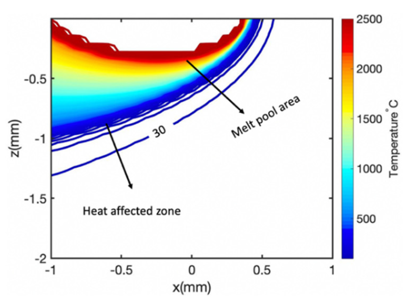
2.1. Thermal Analysis

In this section, a transient three-dimensional heat source model is used to predict the temperature field as:
T   =   P η 8 ρ C p m ( π D t ) 3 / 2 0 t exp ( ( ( x x ) V ( t t ) ) 2 + ( y y ) 2 + ( z z ) 2 4 D ( t t ) ) ( t t ) 3 / 2 d t + T 0
This equation is obtained by solving the differential equation of heat conduction as explained in [24], where P is the laser power, η is the absorption coefficient,   ρ is the density, C p m is the modified heat capacity to consider the latent heat of fusion for solid-state phase change as explained in the work of Mirkoohi et al. [24]. V is the scan speed, D is the thermal diffusivity, and T 0   is the initial temperature.
It should be noted that the proposed method does not model the evaporation. Moreover, it is in semi-infinite medium, thus the impact of geometry is neglected.

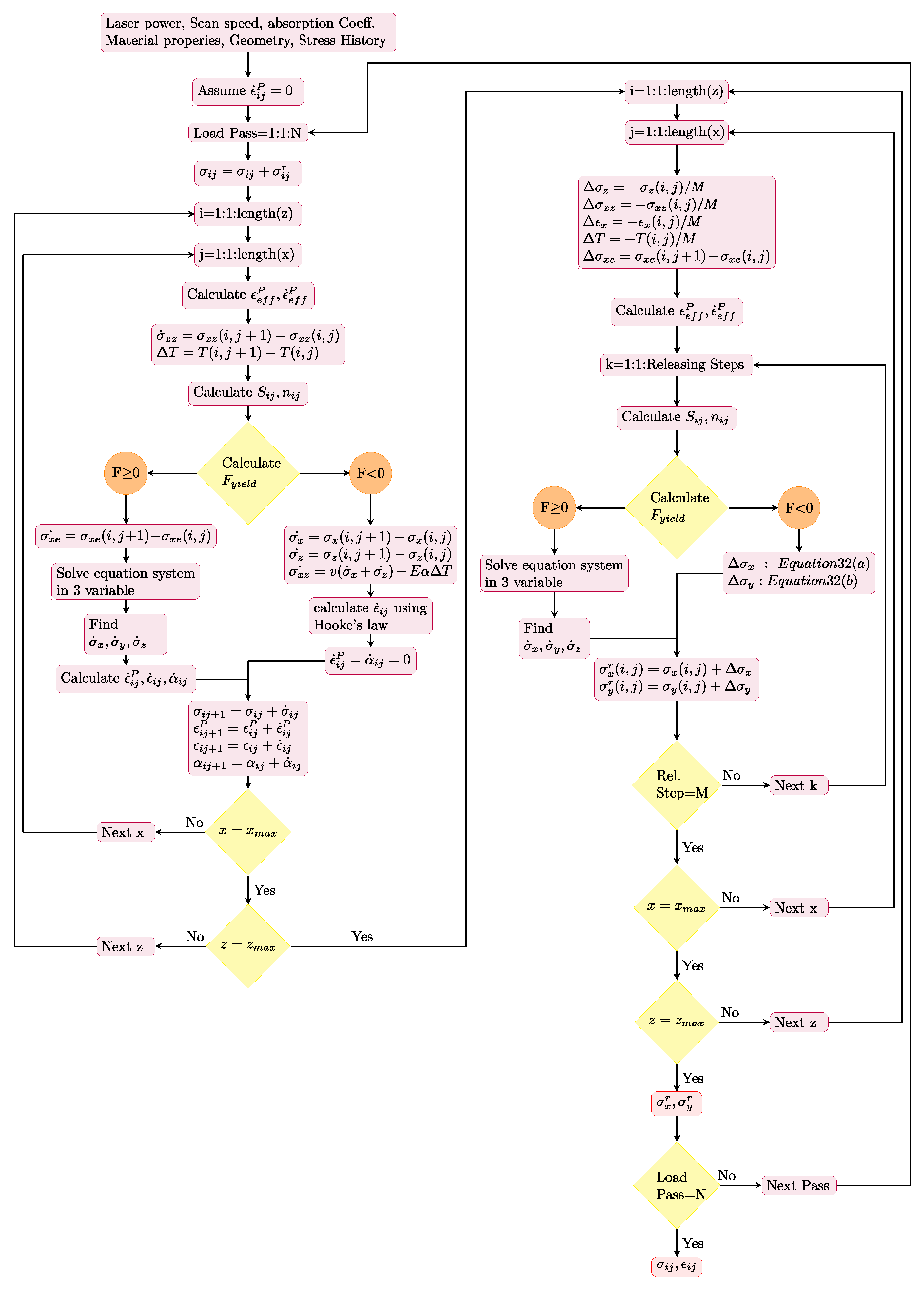
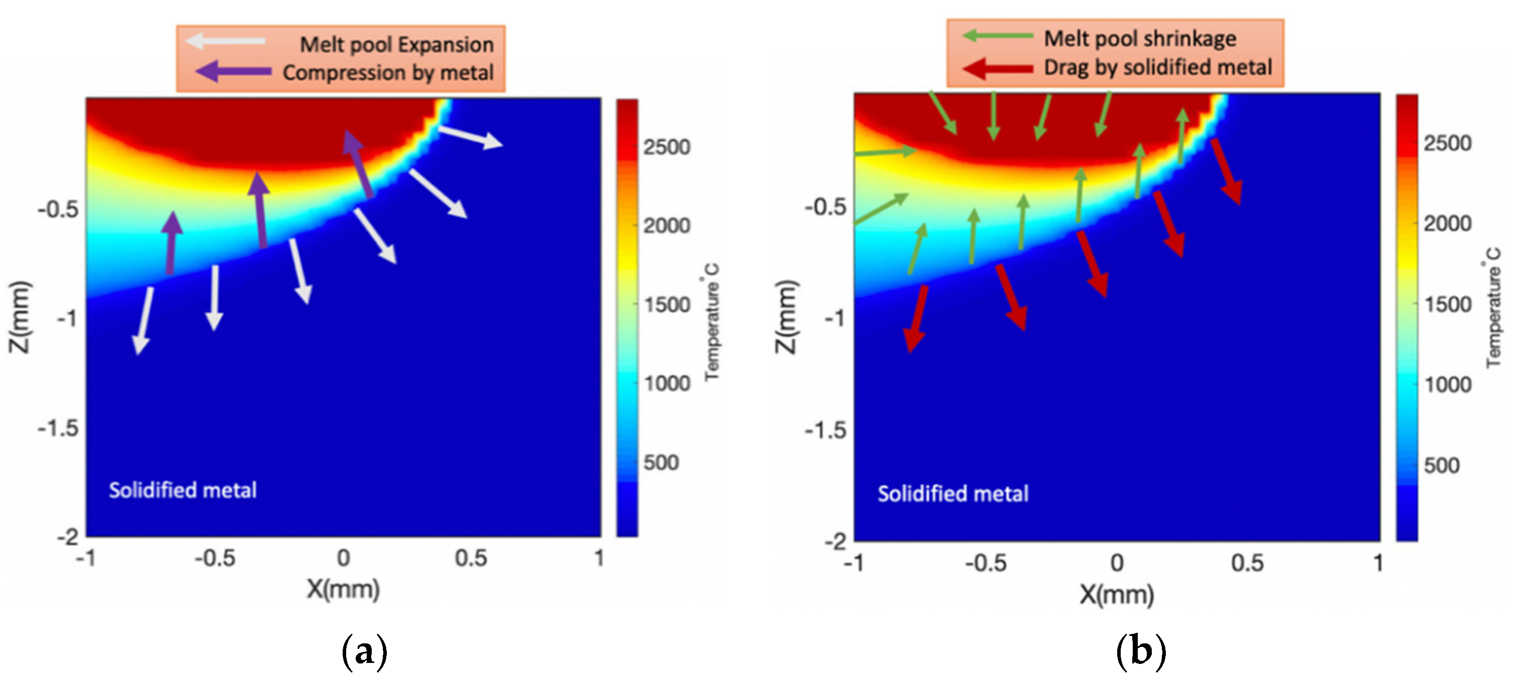
2.2. Mechanical Analysis

A steep temperature gradient and fast solidification may induce thermal stress. The resulting stress is calculated by the combination of the different sources of stresses due to the body forces, normal stress tension, and hydrostatic stress as described by Saif et al. [30]:
σ x x ( x , z )   =   α ( T ) E ( T ) 1 2 ν ( T ) 0 ( G x h T x ( x , z ) + G x v T z ( x , z ) ) d x d z + 2 z π p ( s ) ( s x ) 2 ( ( s x ) 2 + z 2 ) 2 d s α ( T ) E ( T ) T ( x , z ) 1 2 ν ( T )
σ z z ( x , z )   =   α ( T ) E ( T ) 1 2 ν ( T ) 0 ( G z h T x ( x , z ) + G z v T z ( x , z ) ) d x d z + 2 z 3 π p ( s ) ( ( s x ) 2 + z 2 ) 2 d s α ( T ) E ( T ) T ( x , z ) 1 2 ν ( T )
σ x z ( x , z )   =   α ( T ) E ( T ) 1 2 ν ( T ) 0 ( G x z h T x ( x , z ) + G x z v T z ( x , z ) ) d x d z + 2 z 2 π p ( s ) ( s x ) ( ( s x ) 2 + z 2 ) 2 d s
σ z z ( x , z )   =   ν ( T ) ( σ x x + σ z z )   α ( T ) E ( T ) T ( x , z )
where α is the coefficient of thermal expansion, E represents the elastic modulus,   T x is the temperature gradient, ν is Poisson’s ratio, ( G x h ,   G x v , G z h , G z v , G x z h , G x z v ) are the plane strain Green’s function as explained in Appendix A, and p ( s ) is expressed by [31,32]:
p ( s )   =   α ( T ) E ( T ) T ( x , z   =   0 ) 1 2 ν ( T )
At elevated temperatures, the yield strength of Ti-6Al-4V approaches zero. Thus, the AM part experiences a high magnitude of plastic deformation due to heating cycles and cooling cycles [33]. If the stress passes the yield strength, upon unloading (cooling in this situation) some amount of stress remains in the body, which is known as RS. The RS is inherent in all the AM parts and can be reduced or eliminated with proper control and optimization of process parameters or post-processing techniques such as pitting, and heat treatment since it has an elastic nature [34,35].
Both the in-plane and out-of-plane RS distributions are obtained from incremental plasticity and kinematic hardening behavior of metal according to the conservation of volume in plastic deformation in coupling with equilibrium and compatibility conditions. McDowell et al. [36] proposed an algorithm to predict the RS in a rolling process. This algorithm has several advantages, including high computational efficiency and rapid and accurate prediction of RS; however, this algorithm has several limitations and should be modified for the AM applications. First, the stress along the build direction ( σ z z ) is assumed to be elastic. In AM processes, the stress along the build direction has a high magnitude. Thus, the stress along the build direction should be solved simultaneously with σ x x , and σ y y . In this case, there are two equations with three unknowns, which cannot be solved using the McDowell model. Second, this algorithm does not consider the conservation of volume in plastic deformation. Qi et al. [37] explained that these limitations may reduce the precision of the predicted RS.
The Johnson Cook flow stress model is used to determine the yield surface.
k   =   1 3 ( A + B ε e f f p n ) ( 1 + C l n ( ε ˙ e f f p ε ˙ 0 ) ) ( 1 [ T T 0 T m T 0 ] m )
where k is the material yield stress, ε e f f   p represents the effective plastic strain, ε ˙ e f f p is the effective plastic strain rate,   T is the temperature of material, T m is the melting point of material, and T 0 is the initial temperature. The terms A , B ,   C , n , m   and   ε ˙ 0 are the material constants which are listed in Table 1 for Ti-6Al-4V.
If the obtained yield stress passes the yield threshold of the material, then the total plastic strain can be calculated incrementally. The plastic strain rate can is introduced by Khan and Huang [39] as
ε ˙ i j P   =   1 h S k l ˙ n k l n i j
where S k l is deviatoric stress, < > is the MacCauley bracket and is expressed as x   =   0.5 ( x + | x | ) , n i j   =   S i j α i j 2   k , and h is the plastic modulus.
As mentioned before, the previous state of the art algorithm assumed the stress along the build direction (z-direction) is elastic and ignored the volume conservation in plastic deformation. Below we explain how these two limitations can be solved by considering the elastic and plastic components of strain rate in all three directions. In the elastoplastic loading the total strain rate is a combination of the elastic part and the plastic part as:
ε ˙ x x   =   ε ˙ x x e +   ε ˙ x x p
ε ˙ y y   =   ε ˙ y y e +   ε ˙ y y p
ε ˙ z z   =   ε ˙ z z e +   ε ˙ z z p
According to the conservation of volume in plastic deformation:
ε ˙ x x p + ε ˙ y y p + ε ˙ z z p   =   0 .
Based on the plain strain assumption
ε ˙ y y e   = ε ˙ y y p   =   0 ,
then
ε ˙ x x p + ε ˙ z z p   =   0 .
Taking the plastic flow rule (Equation (5)) into Equation (9):
1 h S k l ˙ n k l ( n x x + n z z )   =   0
Based on the plastic loading condition:
S k l ˙ n k l > 0 ,
therefore
( n x x + n z z ) = 0 .
Taking n i j   =   S i j α i j 2   k , and S i j   =   σ i j ( σ k k 3 ) δ i j into Equation (10):
σ y y   =   1 2 ( σ x x + σ z z ) .
The incremental form of Equation (13) can be written as:
σ ˙ y y   =   1 2 ( σ ˙ x x + σ ˙ z z )
Then, by solving three equations with three unknowns, ( σ x x , σ y y , σ z z ) can be obtained as:
{ 1 E [ σ ˙ x x υ ( σ ˙ y y σ ˙ z z ) ] + α Δ T + 1 h ( σ ˙ x x n x x + σ ˙ y y n y y + σ ˙ z z n z z + 2 σ ˙ x z * n x z ) n x x   =   ψ ( 1 E [ σ ˙ x x * υ ( σ ˙ y y σ ˙ z z * ) ] + α Δ T + 1 h ( σ ˙ x x * n x x + σ ˙ y y n y y + σ ˙ z z * n z z + 2 σ ˙ x z * n x z ) n x x ) 1 E [ σ ˙ y y υ ( σ ˙ x x σ ˙ z z ) ] + α Δ T + 1 h ( σ ˙ x x n x x + σ ˙ y y n y y + σ ˙ z z n z z + 2 σ ˙ x z * n x z ) n y y   =   0 σ ˙ y y   =   1 2 ( σ ˙ x x + σ ˙ z z )
where σ ˙ x x * ,   σ ˙ z z * , σ ˙ x z * are the elastic thermal stresses calculated from Equations (2) and (3). The term ψ is the hybrid function which depends on the modulus ratio ( h / G ) as:
ψ   =   1 exp ( ξ 3 h 2 G ) ,
where ξ   =   0.15 is the algorithm constant, and G   =   E / ( 2 ( 1 + υ ) ) is the elastic shear modulus. Three systems of equations are solved simultaneously for σ ˙ x x , σ ˙ y y , and σ ˙ z z for each elastic-plastic increment of strain. Figure 3 illustrates the flow chart of the proposed algorithm.

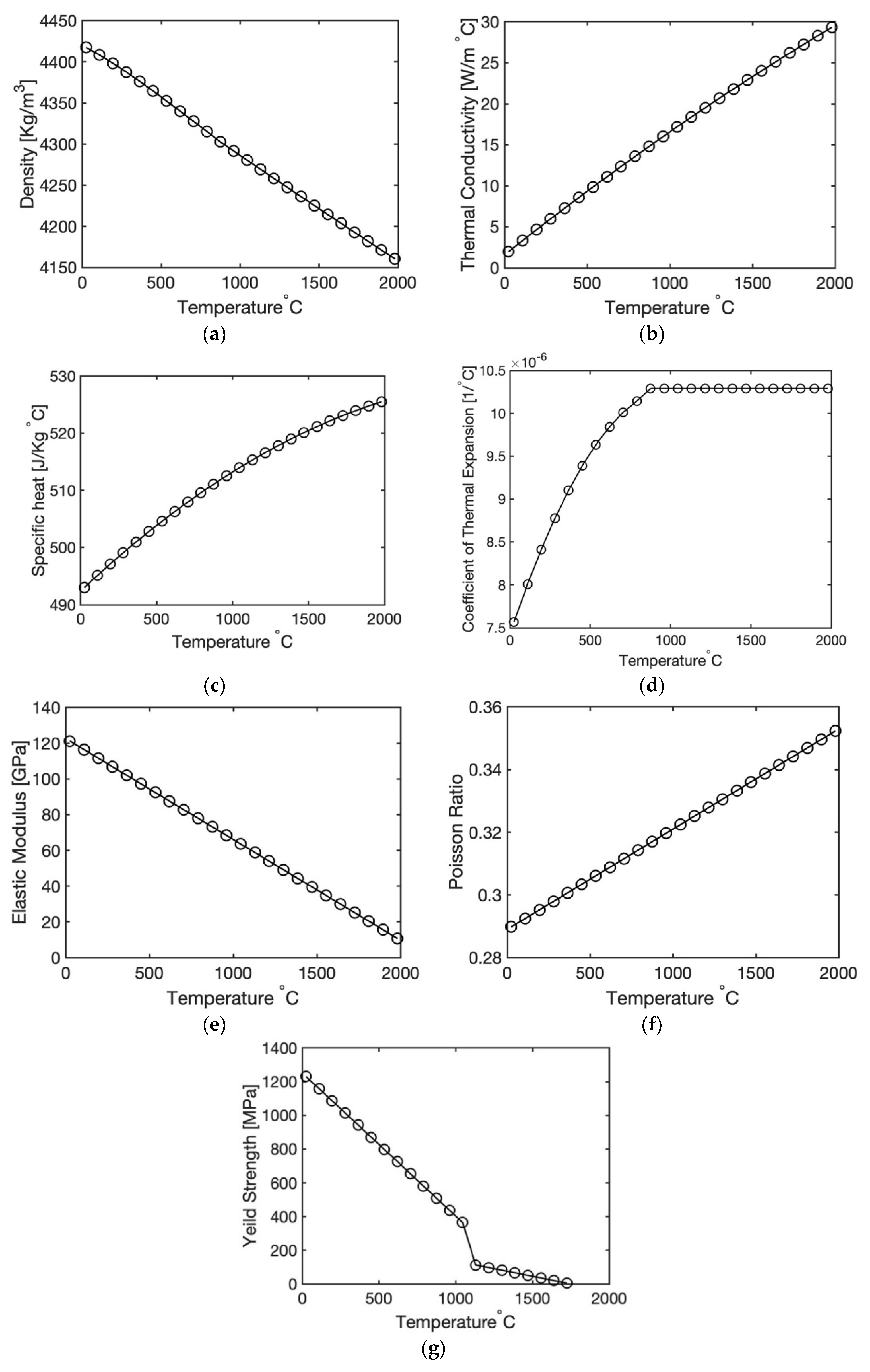
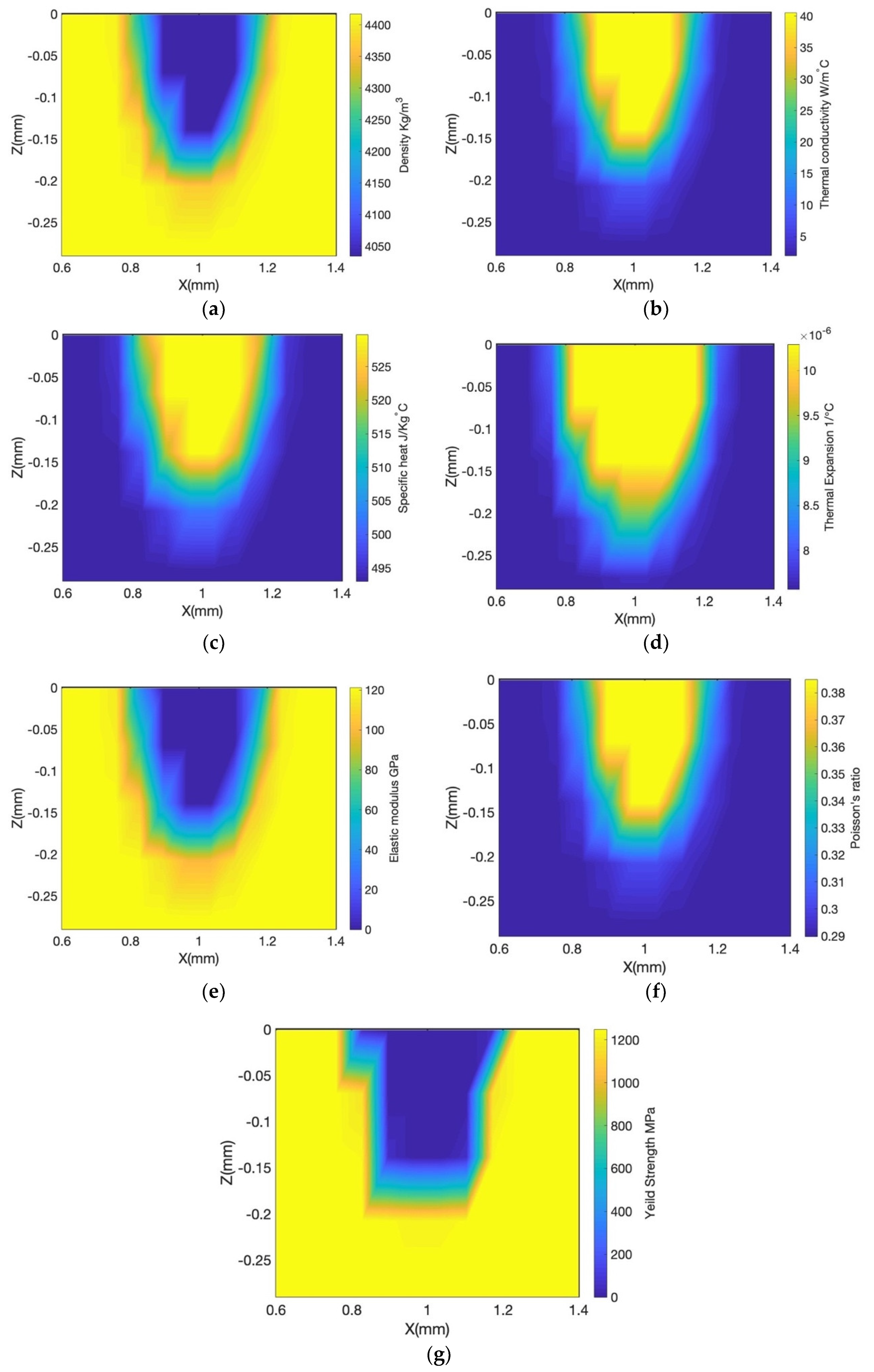
3. Temperature Dependent Material Properties

Due to the rapid heating and low conductivity, materials experience a steep temperature gradient. As a result of the steep temperature gradient, material properties could vary significantly in the medium. Therefore, it is crucial to consider material properties as temperature-dependent. Density, conductivity, specific heat, yield strength, Young’s modulus, Poisson’s ratio, and the thermal expansion coefficient of Ti-6Al-4V are considered to be temperature-sensitive, as shown in Figure 4. These data are gathered from the work of Welsch et al. [40], Heigel et al. [41], Jamshidinia et al. [42], Li et al. [43], Mills [44], and Murgau [45]. The melting temperature range of Ti-6Al-4V is from 1600 to 1660 °C. In this modeling melting temperature is 1600 °C. The density of Ti-6Al-4V drops for about 6.7% from room temperature to 2000 °C; thermal conductivity increases as the temperature increases; the specific heat increases gradually with the increase in temperature; the coefficient of thermal expansion increases gradually up to 1000 °C and reaches a constant value; and the elastic modulus decreases with the increase in temperature and approaches zero at around melting temperature. This shows that the material at liquid phase has negligible elasticity. Poisson’s ratio increases with the increase in temperature; yield strength decreases rapidly from room temperature up to 1000 °C and then the slope slows above 1000 °C. This signifies that the Ti-6Al-4V is extremely soft and it quite easily undergoes plastic deformation at elevated temperatures, which causes the medium to experience high residual stress.
The equations of temperature sensitive material properties are also derived from the data points as listed in Table 2.

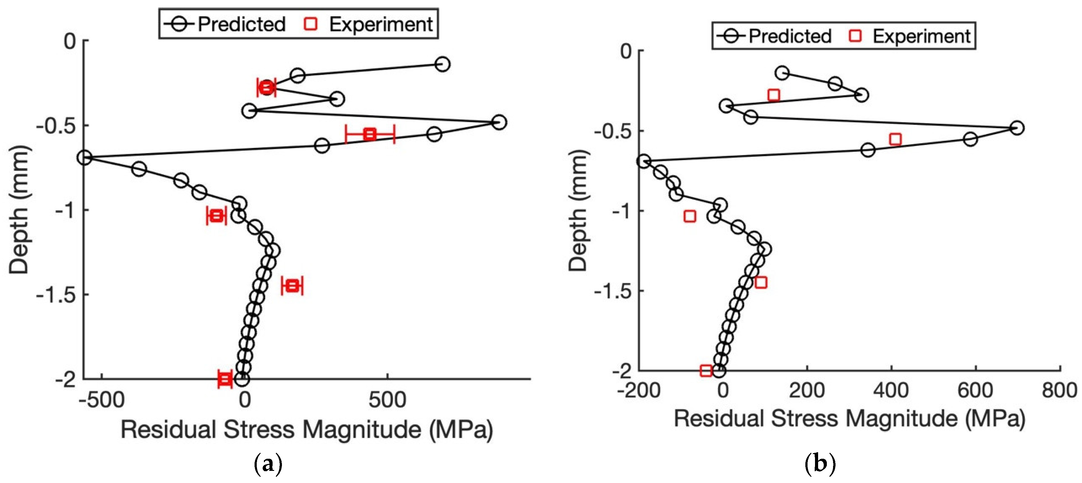
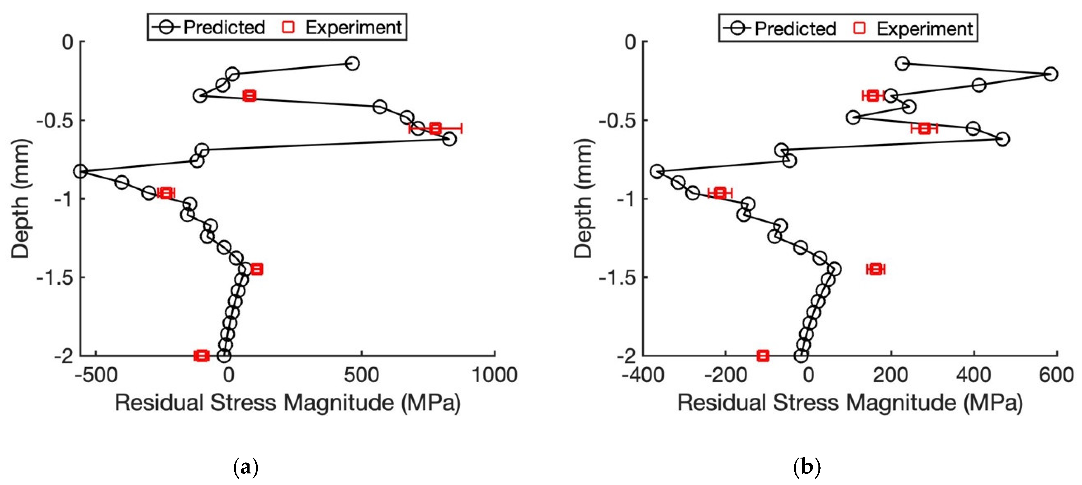
4. Experimental Residual Stress Analysis

Two blocks of Ti-6Al-4V specimens with the size of 20 × 10 × 3 mm were produced via the DMD process using LENS CS 1500 SYSTEMS under different process conditions as shown in Table 3. The selected laser powers were 206 and 385 W, and the scan speeds were 25 and 40 mm/s, respectively. The deposited layer thickness for both samples was 250 μ m ,   and hatch spacing was 105 μ m . A bi-directional continuous scan strategy was used to build the parts as shown in Figure 2.
A PANalytical Empyrean multipurpose X-ray diffractometer was used to measure the RS of the specimens using the s i n 2 Ψ method [46,47]. The residual strains are determined as
ε   =   d d 0 d 0
where, d and d 0 are the stressed and unstressed lattice parameters, respectively.
The generalized Hook’s law for isotropic material is used to calculate stress as
σ i   =   E ( 1 + υ ) ( 1 2 υ ) ( 1 υ ) ε i + υ ( ε j + ε k )   where   i , j , k x , y , z .
In Equation (18), an elastic modulus ( E ) , and Poisson’s ratio of 114 GPa and 0.33 are used, respectively. Samples are polished using liquid abrasive of 1 and 0.05 μ m at a very slow speed to eliminate macroscopic residual stresses. Measurements are collected every 0.5 mm along the build direction (z-axis) of the samples.

5. Results and Discussion

Figure 5 illustrates the melt pool area and the heat-affected zone induced by highly localized heat input and low thermal conductivity. Non-uniform heating induces non-uniform thermal expansion. During the heating cycle, the melt pool area and the heat-affected zone are trying to expand; however, they are surrounded by solidified metal. This would generate the compressive stress state within the melt pool and heat-affected zones as shown in Figure 6a. During the cooling cycle, the shrinkage of the material would develop a tensile stress state as illustrated in Figure 6b.
The proposed analytical model is extremely valuable since it provides a fast (less than 45 s with a 4-processor laptop) and accurate prediction of the stress state within the build. In this modeling, first, a transient moving heat source approach is used to predict the temperature field in AM. Second, the thermal stress induced is calculated by combining three stresses known as stresses due to body forces, normal tension, and hydrostatic stress. Lastly, the stresses may exceed the yield point and the material would experience plastic deformation. As a consequence of repeated loading and unloading (heating and cooling), the material experiences high RS. Therefore, both the in plane and out of plane RS distributions are calculated from the incremental plasticity and kinematic hardening behavior of the metal, based upon the premises of the plane strain condition in the build of isotropic and homogeneous properties, in coupling with the equilibrium and compatibility conditions.
Material properties could vary significantly from point to point due to the steep temperature gradient. Consequently, it is not a fair assumption to consider the material properties constant. Herein, the thermal and mechanical material properties are temperature sensitive. Moreover, in this process, the material experiences cyclic melting and solidification. The energy needed for the phase change is taken into account by incorporating the latent heat of fusion into the specific heat. Furthermore, the multi-layer and multi-scan aspect of metal AM are considered by including the temperature histories from the previous layers and scans.
Experimental measurements are conducted via X-ray diffraction to measure the RS in Ti-6Al-4V specimens built via the DMD process at the middle of the specimens (X = 10 mm, Y = 1.5 mm) along the build direction (z-axis), every 0.5 mm. The scan strategy in both experimentation and analytical modeling is bi-directional. Moreover, the hatching space and layer thickness are 105 and 250 μ m , respectively. Comparison of the results from the proposed analytical model and the experimentation of the Ti-6Al-4V specimens built via the DMD process showed good qualitative and quantitative agreement.
Figure 7 illustrates the predicted temperature field for the Ti-6Al-4V specimens. Figure 7a demonstrates the predicted melt pool area and the heat-affected zone (HAZ) for the first specimen in Table 3, which has a laser power of 206 W and a scan speed of 25 mm/s, with a layer height and hatch spacing of 250 and 105 μ m , respectively. It should be noted that the absorption ratio is 30% for Ti-6Al-4V samples as explained in the work of Selvan et al. [48]. Since the evaporation of the metallic powders is not considered in the modeling, the maximum temperature does not go beyond the evaporation temperature, which is around 3000 °C for Ti-6Al-4V, as reported by Selvan et al. [48]. In this figure, the melt pool depth is around 0.1 mm, based on the melting point of 1600 °C, and the depth of the heat-affected zone is around 0.15 mm. Below this depth, the material is not affected by the laser. The rapid temperature change at the border of HAZ and the completely solid material—which is not affected by the laser—is the region where the stress state within the build part changes from tensile to compressive. This phenomenon will be explained in detail in the following sections of this manuscript. Figure 7b illustrates the predicted temperature field for the second specimen, with the laser power of 385 W, scan speed of 40 mm/s, layer height of 250 μ m and hatch spacing of 105 μ m . Based on the melting point of Ti-6Al-4V (1600 °C), the melt pool depth is 0.14 mm and the HAZ depth is around 0.21 mm. The proposed temperature model is validated in the previous work of Mirkoohi et al. [24].
As explained before. material properties vary significantly since the temperature gradient is quite high in AM. The variation of thermal and mechanical material properties for the second specimen with the laser power of 385 W and scan speed of 40 mm/s is illustrated in Figure 8. The density of the solid material is around 4400 kg / m 3 . As the temperature increases the density decreases to 4050 kg / m 3 in the liquid zone; in the melt pool zone, thermal conductivity reaches its maximum value due to the high magnitude of temperatures, and decreases to around 5 W / m   ° C in the solid zone; the specific heat has the highest magnitude of 530 J / Kg   ° C at the melt pool area and drops to 480 J / Kg   ° C when the material is solidified; thermal expansion is more expanded in the liquid zone compared to other properties, which shows that the thermal expansion is more sensitive to temperature, and it has the highest magnitude in the liquid zone; the elastic modulus in the liquid zone is almost zero, in the HAZ reaches 60 GPa, and in the solid zone it reaches the maximum value of 120 GPa; Poisson’s ratio in the liquid zone has the magnitude of 0.38, and in the solid zone has the value of 0.29; yield strength reaches almost zero in the liquid zone and has the maximum value of 1200 MPa in the solid zone.
Residual stress along the scan direction and transverse direction is predicted using the proposed model and validated experimentally. Figure 9 illustrates the predicted RS along the scan direction and transverse direction as a function of depth into the build part for the first sample with the laser power of 206 W, scan speed of 25 mm/s, layer height of 250 μ m , and hatch spacing of 105 μ m . Since the samples have a rough surface, the top surface of the samples is polished up to 100 μ m with an electromechanical polishing to be able to accurately measure the RS on the surface.
Both the in plane and out of plane residual stresses are highly tensile in the melt pool zone and the heat-affected zone in coherence with most of the reported results in the literature as explained in the introduction section. As shown in Figure 9 and Figure 10, in both the scan direction and the transverse direction, there is a gradual change in the stress state from tensile to compressive. This change occurs at around the depth where the medium is solidified and is not affected by the laser. The results confirm that upon cooling the melt pool and the heat-affected zones are under tension due to the shrinkage of the material, and when the material is completely solidified and is not affected by the laser anymore, the material experiences a compression stress state. The oscillations in the melt pool and the heat-affected zone are due to the fact that the thermal and mechanical material properties vary significantly in these regions. Therefore, an abrupt change in one of the material properties would result in oscillations. This could be better improved by having more material property data points at different temperatures.
Figure 10 shows the predicted RS in the scan and transverse directions for the second sample in Table 2 with the laser power of 385 W, scan speed of 25 mm/s, and layer height and hatch spacing of 250 and 105 μ m , respectively. The stress state is tensile in both the scan and transverse directions and changes to compressive at the depth of around 0.9 mm. Around this region the material is completely solidified and is not affected by the laser. Comparison of the predicted and measured RS shows that they follow each other closely.

6. Conclusions

A physics-based analytical model is proposed to rapidly and accurately calculate the stress state within the additively manufactured part. As the explicit computation is executed without meshing or iteration, it can be completed at a speed several orders of magnitude higher than that of conventional FEMs. The high computational efficiency of the proposed model has the potential to affect a wide range of applications, as it could become a powerful tool for design and also fatigue assessment of components undergoing cyclic loading. It also enables efficient control and optimization of the process parameters, to achieve a high-quality part.
In this modeling, a transient moving point heat source is employed to predict the in-process temperature field within the built part. Thermal stress induced by steep temperature gradient is then obtained using the Green’s functions of stresses due to the point body load in a homogeneous semi-infinite medium. Lastly, the stress state is obtained by importing the thermal history as an input for residual stress prediction using the modified McDowell algorithm, in which both the in plane and out of plane residual stress distributions are obtained from the incremental plasticity and kinematic hardening behavior of the metal, coupled with the equilibrium and compatibility conditions. In this modeling, the relationship between three normal stresses are considered according to the property of volume invariance in plastic deformation.
Due to the fast irradiation of the laser and quite low thermal conductivity of the material, the material experiences a high temperature gradient. The high temperature gradient induced variation of the material properties in the medium. Consequently, the material properties are considered temperature sensitive. Moreover, the energy needed for the solid-state phase change is considered by modifying the heat capacity using the latent heat of fusion. Furthermore, the effect of the layer thickness, the hatching space and the scan strategy are considered in this modeling by incorporating the temperature history from the previous scans.
In this work, first the temperature field is predicted for the Ti-6Al-4V specimens. Distribution of thermal and mechanical material properties including density, specific heat, thermal conductivity, elastic modulus, coefficient of thermal expansion, yield strength, and Poisson’s ratio for the laser power of 385 W and scan speed of 40 mm/s showed that the high temperature gradient in the AM process notably changes the material properties within the medium.
The predicted temperature fields for both samples showed that in the vicinity of the melt pool area the temperature and the magnitude of the temperature gradient is high enough to cause the thermal stress to exceed the yield strength of the material. Upon cyclic loading and unloading of the material during the heating and cooling cycles, the material experience high residual stress. The predicted residual stress showed that the stress state is highly tensile in the melt pool and the heat-affected zones, and compressive in the solidified regions. Good qualitative and quantitative agreement is achieved between the predicted and measured residual stresses for the Ti-6Al-4V samples.

Author Contributions

Conceptualization, E.M.; methodology, E.M.; software, E.M.; validation, E.M.; formal analysis, E.M.; investigation, E.M.; resources, E.M., S.Y.L., D.L., H.G.; data curation, E.M.; writing—original draft preparation, E.M.; writing—review and editing, E.M., S.Y.L.; visualization, E.M.; supervision, S.Y.L. All authors have read and agreed to the published version of the manuscript.

Funding

This research received no external funding.

Conflicts of Interest

The authors declare no conflict of interest.

Appendix A

Elements of the G matrix.
Let X m   =   x x ,   Z P   =   z + z ,   Z m   =   z z ,
As explained by Saif et al. [30], “the Green functions G x h ( x , z , x , z ) and G x v ( x , z , x , z ) are the normal stress due to a unit point body load acting at ( x , z ) along the x and z directions, respectively”.
G x h   = 1 4 π 1 2 ν 1 ν [ 3 2 ν 1 2 ν ( X m X m 2 + Z p 2 X m X m 2 + Z m 2 ) + 2 1 2 ν ( X m Z m 2 ( X m 2 + Z m 2 ) 2 X m Z p 2 ( X m 2 + Z p 2 ) 2 ) ] 1 π 1 1 ν × ( ( 3 2 ν ) X m ( z Z p + X m 2 ) ( X m 2 + Z p 2 ) 2 3 z 2 X m Z p 2 + X m 3 ( 4 z 2 + 6 z z + z 2 + X m 2 ) ( X m 2 + Z p 2 ) 3 )
G z h   = 1 4 π 1 2 ν 1 ν [ ( X m X m 2 + Z p 2 X m X m 2 + Z m 2 ) + 2 1 2 ν ( X m Z m 2 ( X m 2 + Z m 2 ) 2 X m Z p 2 ( X m 2 + Z p 2 ) 2 ) ] 1 π y 1 ν × ( ( 3 2 ν ) X m Z p ( X m 2 + Z p 2 ) 2 X m ( 4 z 3 + 9 z z 2 + 6 z 2 z + z 3 + z X m 2 ( X m 2 + Z p 2 ) 3 )
G x z h   = 1 4 π 1 2 ν 1 ν [ ( Z P X m 2 + Z p 2 Z m X m 2 + Z m 2 ) + 2 1 2 ν ( Z p X m 2 ( X m 2 + Z p 2 ) 2 Z m X m 2 ( X m 2 + Z m 2 ) 2 ) ] 1 π 1 1 ν × ( ( 3 2 ν ) z Z p 2 + X m 2 ( 2 z + z ) 2 ( X m 2 + Z p 2 ) 2 z 3 ( z 2 + 3 z z + 3 z 2 ) + z 3 z 2 + X m 2 ( z 3 + 6 z z 2 + 6 z 2 z + z 3 ) + z X m 4 ( X m 2 + Z p 2 ) 3 )
G x v   = 1 4 π 1 2 ν 1 ν [ ( Z P X m 2 + Z p 2 Z m X m 2 + Z m 2 ) + 2 1 2 ν ( Z m X m 2 ( X m 2 + Z m 2 ) 2 Z p X m 2 ( X m 2 + Z p 2 ) 2 ) ] 1 2 π 1 1 ν × ( 2 ( 1 ν ) Z p ( X m 2 + Z p 2 ) [ 2 ( 1 ν ) z z ] ( Z p 2 X m 2 ) ( X m 2 + Z p 2 ) 2 + 2 z z Z p ( 3 X m 2 Z p 2 ) ( X m 2 + Z p 2 ) 3 )
G z v   = 1 4 π 1 1 ν [ ( 3 2 ν ) ( Z P X m 2 + Z p 2 Z m X m 2 + Z m 2 ) + 2 ( Z m X m 2 ( X m 2 + Z m 2 ) 2 Z p X m 2 ( X m 2 + Z p 2 ) 2 ) ] 1 2 π 1 1 ν × ( 2 ( 1 ν ) Z p ( X m 2 + Z p 2 ) + [ 2 ( 1 ν ) z + z ] ( Z p 2 X m 2 ) ( X m 2 + Z p 2 ) 2 2 z z Z p ( 3 X m 2 Z p 2 ) ( X m 2 + Z p 2 ) 3 )
G x z v   = X m 4 π 1 2 ν 1 ν [ ( 1 X m 2 + Z p 2 1 X m 2 + Z m 2 ) + 2 1 2 ν ( Z p 2 ( X m 2 + Z P 2 ) 2 Z m 2 ( X m 2 + Z m 2 ) 2 ) ] X m 2 π 1 1 ν × ( 4 ( 1 ν ) z Z p ( X m 2 + Z p 2 ) 2 + 2 z z Z p ( 3 Z p 2 X m 2 ) ( X m 2 + Z p 2 ) 3 )

References

  1. Herderick, E. Additive manufacturing of metals: A review. Mater. Sci. Technol. 2011, 2, 1413–1425. [Google Scholar]
  2. Namatollahi, M.; Jahadakbar, A.; Mahtabi, M.J.; Elahinia, M. Additive manufacturing (AM). In Metals for Biomedical Devices; Elsevier: Amsterdam, The Netherlands, 2019; pp. 331–353. [Google Scholar]
  3. Camacho, D.D.; Clayton, P.; O’Brien, W.J.; Seepersad, C.; Juenger, M.; Ferron, R.; Salamone, S. Applications of additive manufacturing in the construction industry—A forward-looking review. Autom. Constr. 2018, 89, 110–119. [Google Scholar] [CrossRef]
  4. Ngo, T.D.; Kashani, A.; Imbalzano, G.; Nguyen, K.T.; Hui, D. Additive manufacturing (3D printing): A review of materials, methods, applications and challenges. Compos. Part B Eng. 2018, 143, 172–196. [Google Scholar] [CrossRef]
  5. Ji, X.; Mirkoohi, E.; Ning, J.; Liang, S.Y. Analytical modeling of post-printing grain size in metal additive manufacturing. Opt. Lasers Eng. 2020, 124, 105805. [Google Scholar] [CrossRef]
  6. Tabei, A.; Mirkoohi, E.; Garmestani, H.; Liang, S. Modeling of texture development in additive manufacturing of Ni-based superalloys. Int. J. Adv. Manuf. Technol. 2019, 103, 1057–1066. [Google Scholar] [CrossRef]
  7. Bartlett, J.L.; Croom, B.P.; Burdick, J.; Henkel, D.; Li, X. Revealing mechanisms of residual stress development in additive manufacturing via digital image correlation. Addit. Manuf. 2018, 22, 1–12. [Google Scholar] [CrossRef]
  8. Roehling, J.D.; Smith, W.L.; Roehling, T.T.; Vrancken, B.; Guss, G.M.; McKeown, J.T.; Hill, M.R.; Matthews, M.J. Reducing residual stress by selective large-area diode surface heating during laser powder bed fusion additive manufacturing. Addit. Manuf. 2019, 28, 228–235. [Google Scholar] [CrossRef]
  9. Wang, Z.; Denlinger, E.; Michaleris, P.; Stoica, A.D.; Ma, D.; Beese, A.M. Residual stress mapping in Inconel 625 fabricated through additive manufacturing: Method for neutron diffraction measurements to validate thermomechanical model predictions. Mater. Des. 2017, 113, 169–177. [Google Scholar] [CrossRef] [Green Version]
  10. An, K.; Yuan, L.; Dial, L.; Spinelli, I.; Stoica, A.D.; Gao, Y. Neutron residual stress measurement and numerical modeling in a curved thin-walled structure by laser powder bed fusion additive manufacturing. Mater. Des. 2017, 135, 122–132. [Google Scholar] [CrossRef]
  11. Denlinger, E.R.; Heigel, J.C.; Michaleris, P. Residual stress and distortion modeling of electron beam direct manufacturing Ti-6Al-4V. Proc. Inst. Mech. Eng. Part B J. Eng. Manuf. 2015, 229, 1803–1813. [Google Scholar] [CrossRef]
  12. Zhao, X.; Iyer, A.; Promoppatum, P.; Yao, S.-C. Numerical modeling of the thermal behavior and residual stress in the direct metal laser sintering process of titanium alloy products. Addit. Manuf. 2017, 14, 126–136. [Google Scholar] [CrossRef]
  13. Romano, S.; Brückner-Foit, A.; Brandão, A.; Gumpinger, J.; Ghidini, T.; Beretta, S. Fatigue properties of AlSi10Mg obtained by additive manufacturing: Defect-based modelling and prediction of fatigue strength. Eng. Fract. Mech. 2018, 187, 165–189. [Google Scholar] [CrossRef]
  14. Noronha, P.; Wert, J. An ultrasonic technique for the measurement of residual stress. J. Test. Eval. 1975, 3, 147–152. [Google Scholar]
  15. Chung, D. Thermal analysis of carbon fiber polymer-matrix composites by electrical resistance measurement. Thermochim. Acta 2000, 364, 121–132. [Google Scholar] [CrossRef]
  16. Krause, T.W.; Clapham, L.; Pattantyus, A.; Atherton, D.L. Investigation of the stress-dependent magnetic easy axis in steel using magnetic Barkhausen noise. J. Appl. Phys. 1996, 79, 4242–4252. [Google Scholar] [CrossRef]
  17. Ager, J.W., III; Drory, M.D. Quantitative measurement of residual biaxial stress by Raman spectroscopy in diamond grown on a Ti alloy by chemical vapor deposition. Phys. Rev. B 1993, 48, 2601. [Google Scholar] [CrossRef]
  18. Prime, M.B. Cross-sectional mapping of residual stresses by measuring the surface contour after a cut. J. Eng. Mater. Technol. 2001, 123, 162–168. [Google Scholar] [CrossRef] [Green Version]
  19. Aggarangsi, P.; Beuth, J.L. Localized preheating approaches for reducing residual stress in additive manufacturing. In Proceedings of the 2006 International Solid Freeform Fabrication Symposium, Austin, TX, USA, 14–16 August 2006; pp. 709–720. [Google Scholar]
  20. Panda, B.K.; Sahoo, S. Numerical simulation of residual stress in laser based additive manufacturing process. IOP Conf. Ser. Mater. Sci. Eng. 2018, 338, 012030. [Google Scholar] [CrossRef] [Green Version]
  21. Chen, Q.; Liang, X.; Hayduke, D.; Liu, J.; Cheng, L.; Oskin, J.; Whitmore, R.; To, A.C. An inherent strain based multiscale modeling framework for simulating part-scale residual deformation for direct metal laser sintering. Addit. Manuf. 2019, 28, 406–418. [Google Scholar] [CrossRef]
  22. Ganeriwala, R.; Strantza, M.; King, W.; Clausen, B.; Phan, T.; Levine, L.; Brown, D.; Hodge, N. Evaluation of a thermomechanical model for prediction of residual stress during laser powder bed fusion of Ti-6Al-4V. Addit. Manuf. 2019, 27, 489–502. [Google Scholar] [CrossRef]
  23. Ding, H.; Shin, Y.C. A metallo-thermomechanically coupled analysis of orthogonal cutting of AISI 1045 steel. J. Manuf. Sci. Eng. 2012, 134, 051014. [Google Scholar] [CrossRef]
  24. Mirkoohi, E.; Seivers, D.E.; Garmestani, H.; Liang, S.Y. Heat source modeling in selective laser melting. Materials 2019, 12, 2052. [Google Scholar] [CrossRef] [PubMed] [Green Version]
  25. Mirkoohi, E.; Sievers, D.E.; Garmestani, H.; Chiang, K.; Liang, S.Y. Three-dimensional semi-elliptical modeling of melt pool geometry considering hatch spacing and time spacing in metal additive manufacturing. J. Manuf. Process. 2019, 45, 532–543. [Google Scholar] [CrossRef]
  26. Mirkoohi, E.; Ning, J.; Bocchini, P.; Fergani, O.; Chiang, K.-N.; Liang, S. Thermal modeling of temperature distribution in metal additive manufacturing considering effects of build layers, latent heat, and temperature-sensitivity of material properties. J. Manuf. Mater. Process. 2018, 2, 63. [Google Scholar] [CrossRef] [Green Version]
  27. Fergani, O.; Berto, F.; Welo, T.; Liang, S. Analytical modelling of residual stress in additive manufacturing. Fatigue Fract. Eng. Mater. Struct. 2017, 40, 971–978. [Google Scholar] [CrossRef]
  28. Carslaw, H.S.; Jaeger, J.C. Conduction of Heat in Solids, 2nd ed.; Clarendon Press: Oxford, UK, 1959. [Google Scholar]
  29. Goldak, J. A Double Ellipsoid Finite Element Model for Welding Heat Sources. IIW Doc. No. 212-603-85. 1985. Available online: https://ci.nii.ac.jp/naid/10003823699/ (accessed on 1 June 2020).
  30. Saif, M.; Hui, C.; Zehnder, A. Interface shear stresses induced by non-uniform heating of a film on a substrate. Thin Solid Films 1993, 224, 159–167. [Google Scholar] [CrossRef]
  31. Mirkoohi, E.; Dobbs, J.R.; Liang, S.Y. Analytical mechanics modeling of in-process thermal stress distribution in metal additive manufacturing. J. Manuf. Process. 2020, 58, 41–54. [Google Scholar] [CrossRef]
  32. Mirkoohi, E.; Sievers, D.E.; Garmestani, H.; Liang, S.Y. Thermo-mechanical modeling of thermal stress in metal additive manufacturing considering elastoplastic hardening. CIRP J. Manuf. Sci. Technol. 2020, 28, 52–67. [Google Scholar] [CrossRef]
  33. Mirkoohi, E.; Dobbs, J.R.; Liang, S.Y. Analytical modeling of residual stress in direct metal deposition considering scan strategy. Int. J. Adv. Manuf. Technol. 2020, 106, 4105–4121. [Google Scholar] [CrossRef]
  34. Mirkoohi, E.; Tran, H.-C.; Lo, Y.-L.; Chang, Y.-C.; Lin, H.-Y.; Liang, S.Y. Analytical mechanics modeling of residual stress in laser powder bed considering flow hardening and softening. Int. J. Adv. Manuf. Technol. 2020, 107, 4159–4172. [Google Scholar] [CrossRef]
  35. Mirkoohi, E.; Tran, H.-C.; Lo, Y.-L.; Chang, Y.-C.; Lin, H.-Y.; Liang, S.Y. Analytical Modeling of Residual Stress in Laser Powder Bed Fusion Considering Part’s Boundary Condition. Crystals 2020, 10, 337. [Google Scholar] [CrossRef]
  36. McDowell, D. An approximate algorithm for elastic-plastic two-dimensional rolling/sliding contact. Wear 1997, 211, 237–246. [Google Scholar] [CrossRef]
  37. Qi, Z.; Li, B.; Xiong, L. An improved algorithm for McDowell’s analytical model of residual stress. Front. Mech. Eng. 2014, 9, 150–155. [Google Scholar] [CrossRef]
  38. Lesuer, D. Experimental Investigation of Material Models for Ti-6Al-4V and 2024-T3. 2000. Available online: https://e-reports-ext.llnl.gov/pdf/236167.pdf (accessed on 29 December 2015).
  39. Khan, A.S.; Huang, S. Continuum Theory of Plasticity; John Wiley & Sons: Hoboken, NJ, USA, 1995. [Google Scholar]
  40. Welsch, G.; Boyer, R.; Collings, E. Materials Properties Handbook: Titanium Alloys; ASM International: Almere, The Netherlands, 1993. [Google Scholar]
  41. Heigel, J.; Michaleris, P.; Reutzel, E.W. Thermo-mechanical model development and validation of directed energy deposition additive manufacturing of Ti–6Al–4V. Addit. Manuf. 2015, 5, 9–19. [Google Scholar] [CrossRef]
  42. Jamshidinia, M.; Kong, F.; Kovacevic, R. Numerical modeling of heat distribution in the electron beam melting® of Ti-6Al-4V. J. Manuf. Sci. Eng. 2013, 135, 061010. [Google Scholar] [CrossRef]
  43. Li, J.J.; Johnson, W.L.; Rhim, W.-K. Thermal expansion of liquid Ti–6Al–4V measured by electrostatic levitation. Appl. Phys. Lett. 2006, 89, 111913. [Google Scholar] [CrossRef] [Green Version]
  44. Mills, K.C. Recommended Values of Thermophysical Properties for Selected Commercial Alloys; Woodhead Publishing: Cambridge, UK, 2002. [Google Scholar]
  45. Murgau, C.C. Microstructure Model for Ti-6Al-4V Used in Simulation of Additive Manufacturing. Ph.D. Thesis, Luleå University of Technology, Luleå, Sweden, 2016. [Google Scholar]
  46. Nadammal, N.; Kromm, A.; Saliwan-Neumann, R.; Farahbod, L.; Haberland, C.; Portella, P.D. Influence of support configurations on the characteristics of selective laser-melted inconel 718. JOM 2018, 70, 343–348. [Google Scholar] [CrossRef]
  47. Prevey, P.S. X-ray diffraction residual stress techniques. ASM Int. ASM Handb. 1986, 10, 380–392. [Google Scholar]
  48. Selvan, J.S.; Subramanian, K.; Nath, A.; Kumar, H.; Ramachandra, C.; Ravindranathan, S. Laser boronising of Ti–6Al–4V as a result of laser alloying with pre-placed BN. Mater. Sci. Eng. A 1999, 260, 178–187. [Google Scholar] [CrossRef]
Figure 1. Heat transfer model of additive manufacturing (AM) process.
Modelling 01 00015 g001
Figure 2. Illustration of layer height, hatch spacing, and scan strategy.
Modelling 01 00015 g002
Figure 3. Residual stress and relaxation algorithms.
Modelling 01 00015 g003
Figure 4. Temperature-dependent material properties of Ti-6Al-4V: (a) density, (b) thermal conductivity, (c) specific heat, (d) thermal expansion, (e) elastic modulus, (f) Poisson’s ratio, and (g) yield strength.
Modelling 01 00015 g004
Figure 5. Illustration of the melt pool and the heat-affected zone.
Modelling 01 00015 g005
Figure 6. Illustration of the accumulation of stress during: (a) the heating cycle and (b) the cooling cycle.
Modelling 01 00015 g006
Figure 7. Predicted temperature field for Ti-6Al-4V with: (a) laser power = 206 W and scan speed = 25 mm/s and (b) laser power = 385 W and scan speed = 40 mm/s.
Modelling 01 00015 g007
Figure 8. Predicted material properties distribution for Ti-6Al-4V with the laser power of 385 W and scan speed of 40 mm/s: (a) density, (b) conductivity, (c) specific heat, (d) thermal expansion, (e) elastic modulus, (f) Poisson’s ratio and (g) yield strength.
Modelling 01 00015 g008
Figure 9. Predicted residual stress for Ti-6Al-4V with laser power of 206 W, and a scan speed of 25 mm/s along: (a) the scan direction and (b) the transverse direction.
Modelling 01 00015 g009
Figure 10. Predicted residual stress for Ti-6Al-4V with laser power of 385 W, and a scan speed of 40 mm/s along: (a) the scan direction and (b) the transverse direction.
Modelling 01 00015 g010
Table 1. Johnson–Cook parameters for Ti-6Al-4V [38].
A (MPa)B (MPa)Cnm ε ˙ 0
997.9653.10.0250.450.61
Table 2. Thermal and mechanical material properties of Ti-6Al-4V [44].
Density [kg/ m 3 ] ρ = 4420 / ( 1 + α × T ) 3
Thermal conductivity [W/m   ° C ] K = 1.57 + 1.6 e 2 × T 1 e 6 × T 2
Specific heat [J/kg   ° C ] C = 492.4 + 0.025 × T 4.18 e 6 × T 2
Thermal expansion [1/   ° C ] { α = 7.43 e 6 + 5.56 e 9 × T 2.69 e 12 × T 2                  T < 827 α = 10.291 e 6                                                                          T > 827
Elastic modulus [GPa] E = 122.7 0.0565 × T
Poisson’s ratio υ = 0.289 + 3.2 e 5 × T
Yield strength [MPa] { σ Y = 1256 0.8486 × T            T < 1127    σ Y = 316 0.16 × T                  T > 1127
Table 3. Process parameters for direct metal deposition (DMD) of Ti-6Al-4V specimens.
Laser Power
(W)
Scan Speed (mm/s)Feed Rate
(gram/s)
Layer Height
( μ m )
Hatch Spacing ( μ m )
206251250105
385400.5250105
Publisher’s Note: MDPI stays neutral with regard to jurisdictional claims in published maps and institutional affiliations.

