DESIDS: An Integrated Decision Support System for the Planning, Analysis, Management and Rehabilitation of Pressurised Irrigation Distribution Systems

Abstract

Pressurized irrigation distribution systems (PIDSs) play a vital role in irrigation intensification, especially in the Mediterranean region. The design, operation and management of these systems can be complex, as they involve several intertwined processes which need to be considered simultaneously. For this reason, numerous decision support systems (DSSs) have been developed and are available to deal with these processes, but as independent components. To this end, a comprehensive DSS called DESIDS has been developed and tested. This DSS has been developed to bear in mind the needs of irrigation district managers for an integrated tool that can assist them in taking strategic decisions for managing and developing reliable, adequate and sustainable water distribution plans which provide the best services to farmers. Hence, four modules were integrated in DESIDS: (i) irrigation demand and scheduling module; (ii) hydraulic analysis module; (iii) operation and management module; and (iv) design and rehabilitation module. DESIDS was tested on different case studies, proving itself a valuable tool for irrigation district managers, as it provides a wide range of decision options for the proper operation and management of PIDSs. The developed DSS can be used as a platform for future integrations and expansions, and to include other processes needed for better decision-making support.

1. Introduction

The decision-making processes associated with collective pressurized irrigation distribution systems (PIDSs) are very complex and require thorough consideration and analysis. The decision support process for collective distribution systems includes [1]: (i) the determination of the existing problems to be solved and the targeted objectives; (ii) an analysis of the current operation processes (mainly the links between the managers and the farmers’ decisions); (iii) a definition of management plans; and (iv) an assessment of possible operation and management strategies and their expected impact on farmers. Nowadays, irrigation district managers are in need of several tools to assess the performance and the management of PIDSs, such as hydraulic models or decision support systems (DSSs) which are available, but as independent elements [2].

Even though there are many models which have been developed for irrigation and water distribution systems (WDSs), only a few are adopted in practice. For example, Ref. [3] identified some of the reasons why users do not use DSSs, which include: (i) not considering the user in the development of DSSs; (ii) the “black-box” nature of some DSSs; (iii) the cost; (iv) the DSS is not related to “realistic” problems; and (v) the high level of complexity of DDSs. Extensive studies are reported in the literature concerning the development of computer models and DSSs to be used at farm and district levels. The two levels are linked; thus, an adequate DSS has to consider a balanced approach while paying attention to both.

At the farm level, irrigation scheduling models are practically useful for the simulation of alternative irrigation schedules relative to different levels of farmers’ management practices. Many models and software are available to support farmers’ when it comes to the calculation of crop water requirements (CWRs) and determination of irrigation scheduling, such as CROPWAT [4], GISAREG ([5], WISCHE [6] and IRRINET [7].

At a district level, the integration of different models is required as the operation and management of collective distribution systems become more complex. For WDSs, most of the available DSSs deal with the operation, management and rehabilitation of drinking WDSs, focusing on the control of pipe leakages and optimization [8,9,10,11]. In the agricultural sector, Mateos et al. [12] presented SIMIS, Scheme Irrigation Management Information System, a DSS for managing irrigation schemes. SIMIS encompasses two management modules: (i) the water management module, which includes four sub-modules, crop water requirements, irrigation plan, water delivery scheduling and water consumption; and (ii) the financial management module, which includes accounting, water fees and control of maintenance activities in sub-modules. In addition, it comprises a performance assessment sub-module that allows the calculation of several indicators related to water distribution, agricultural intensity, maintenance and financial matters. The water delivery in SIMIS mainly addresses open canal systems and is applicable to only branched irrigation distribution systems. In addition, it can handle three main water delivery modes: fixed rotation, semi-demand and proportional supply. SIMIS has been shown to be a useful tool in the management of irrigation schemes. However, the analysis of more flexible delivery modalities is tedious within SIMIS, and it requires calculations outside of SIMIS [13].

Concerning PIDS, Lamaddalena and Sagardoy [14] presented COPAM, Combined Optimization and Performance Analysis Model, a software package for the design and analysis of large-scale distribution networks. It includes three modules: (i) the generation of demand discharges using the Clément probabilistic method [15]; (ii) the optimization of pipe sizes using Labye’s iterative discontinuous method [16]; and (iii) the analysis of hydraulic performance by randomly generating a large number of open-hydrant configurations. COPAM is also limited to the design and analysis of branched networks.

GESTAR [17] is a computational hydraulic software tool specifically adapted to the design, planning and management of both collective and on-farm pressurized irrigation networks. This tool integrates two main modules: (i) the optimization of branched networks with predefined layouts, using a combination of continuous Lagrange method and discontinuous Labye method [18]; and (ii) a module for hydraulic and energy analysis. This module includes several features such as scenario generation tools with deterministic and random demand states, quasi-steady time evolutions (extended period simulation), computation of accumulated or stochastic flow rates, pumping station and system curve computation, estimation of probability density function of the discharge flow rates and deterministic or stochastic computation of the energy consumed at a pumping station, instantaneously or in a given period. The design optimization in GESTAR is limited to the branched network.

Urrestarazu, Díaz, Poyato, Luque and Jaraba [2] developed an integrated computational tool called INM (Irrigation Networks’ Manager) to assess the distribution networks’ performance and the quality of service provided in an irrigation district. The tool combines GIS, a hydraulic model, EPANET [19] and performance indicators (PIs) to create a database that deals with most information required in an irritation district. Different PIs are calculated using information obtained from hydraulic simulations (simulated measures) and remote data collection systems (real measures). The obtained results, which can be spatially identified and managed, give information about networks’ performances and their response to different conditions to improve performance of irrigation districts.

There are other examples of models and expensive software, which have been developed and that can be used for PIDSs. However, there is no DSS that encompasses all the processes needed by an irrigation district manager to deal with all the issues encountered in PIDSs. Therefore, there is a need to provide an integrated solution, a DSS that is based on a real “need” service that help irrigation district managers with the complex intertwined components of PIDS, such as planning, performance analysis, management and rehabilitation. An effective DSS should incorporate, simultaneously, all these components and must be flexible to adjust to new requirements and changes needed by its user. A DSS should also offer an effective platform for managers to understand the impact of their future decisions on the overall performance of the PIDS and on the quality of services provided to farmers.

The main objective of this work is to develop an integrated DSS tool that will allow irrigation district managers to evaluate options for managing and developing reliable, adequate and sustainable water distribution plans that provide the best service to farmers. This tool will permit the analysis of the hydraulic performance of existing PIDSs, the evaluation of different scenarios for managing these systems, the optimization of system operations and the optimization of rehabilitation plans if needed.

2. DSS Description

The developed DSS, called DESIDS (DEcision Support for Irrigation Distribution Systems), is a stand-alone software written in Microsoft^® Visual Basic^® programming language and supported by a user-friendly Graphical User Interface (GUI) and built-in GIS capabilities (Figure 1). Prodigious care has been taken in creating a flexible, relatively easy to handle software, which could be used in different contexts of PIDS, from planning to management and rehabilitation. DESIDS is set to address the different processes needed for managing collective irrigation systems [1]: operational (daily irrigation scheduling and distribution), tactical (changing systems’ operation without modifying the infrastructures) and strategic (changing structural capacities through new investments, e.g., structural rehabilitation). Therefore, it is set to help irrigation district managers address the different issues identified specifically in their districts.

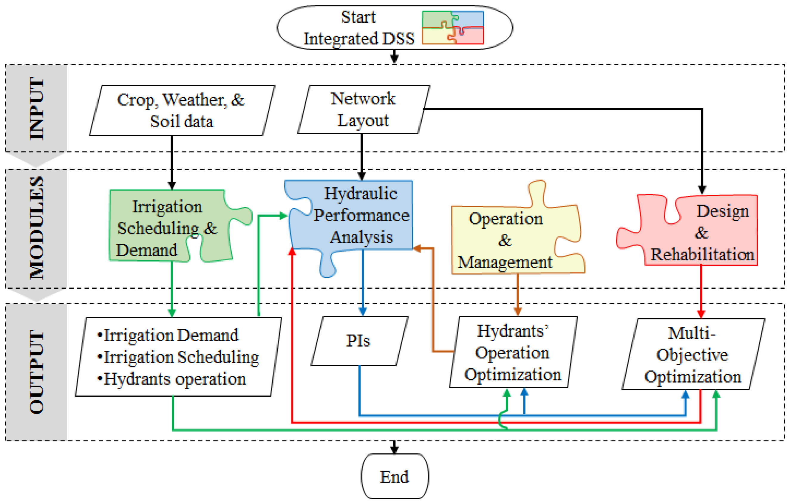
DESIDS encompasses four separate yet easily integrated elements or modules: (i) an irrigation demand and scheduling module that calculates CWR, irrigation demand, irrigation scheduling for an entire irrigation district and generates operating hydrant configurations; (ii) a hydraulic analysis module that uses different PIs to evaluate the performance of a PIDS. The analysis is carried out by either randomly generating a large number of hydrant opening configurations or by using realistic configurations from the previous module; (iii) an operation and management module that provides optimal operation strategies to achieve the best services (demand and pressure) to farmers; and (iv) a rehabilitation module that implements multi-objective optimization for the rehabilitation of existing networks, as well as the design of new ones.

The outputs of each of the above modules are presented in tabular and graphical forms to facilitate the interpretation of the results. Some of the outputs are designed to be used as inputs for one of the available modules to enable the integration and the flow of information in the DSS, as illustrated in Figure 2. Detailed descriptions of the four modules are presented in the following sections.

2.1. Irrigation Demand and Scheduling Module

To evaluate the performance of PIDSs and to take the appropriate decisions concerning the operation and management of these systems, it is necessary to know the allocation of water at the farm level. To this end, the irrigation demand and scheduling module is used to simulate CWR and irrigation scheduling for each field in an irrigation district. The incorporation of this module in DESIDS is imperative, as it allows irrigation system managers to efficiently match available discharges and pressures supplied by the system to on-farm water use. In turn, it allows them to take the necessary decisions to provide adequate PIDSs performance to meet the crop water demands. Irrigation demand and irrigation scheduling are determined following the approach of CROPWAT using climatic, crop and soil parameters. The required data can be entered through the GUI and stored in a database to be retrieved when needed. All the input data and the results are displayed in tabular and graphical form to facilitate their interpretation (Figure 3). The estimation of irrigation requirements is one of the principal parameters for the planning, design and operation of PIDSs. In this module, monthly available data are used for estimating the crop water requirements and irrigation requirements, especially during the peak period, for a proposed cropping pattern. This is vital for the planning and design of a PIDS. The daily data are important for formulating the policy for the optimal allocation of water, as well as in decision making concerning the day-to-day operation and management of the systems. This model was calibrated by comparing the obtained results from the calculation of reference evapotranspiration, irrigation demands and irrigation scheduling with the results obtained using CROPWAT.

2.1.1. Irrigation Requirements

To estimate irrigation requirements, daily (or monthly) reference evapotranspiration (ET₀) has to be provided or calculated using either FAO-56 Penman–Monteith (Equation (1)) or Hargreaves (Equation (2)) methods, depending on the availability of data [20]:

ET₀ = (0.408 ∆ (R_n − G) + (γ 900/(T + 273)) u₂ (e_s − e_a))/(∆ + γ (1 + 0.34 u₂))

(1)

where R_n is the net radiation at the crop surface (MJ m⁻² day⁻¹), G is soil heat flux density (MJ m⁻² day⁻¹), T is the mean daily air temperature at 2 m height (°C), u₂ is the wind speed at 2 m height (m s⁻¹), e_s is the saturation vapour pressure (kPa), e_a is the actual vapour pressure (kPa), (e_s – e_a) is the saturation vapour pressure deficit (kPa), Δ is the slope vapour pressure curve (kPa °C⁻¹) and γ is the psychrometric constant (kPa °C⁻¹).

ET₀ = 0.0023 (T + 17.8) (T_max – T_min)^0.5 R_a

(2)

where T_max and T_min are, respectively, the maximum and minimum temperatures (°C) and R_a is the extraterrestrial radiation (mm day⁻¹).

It is worth mentioning that the values of crop evapotranspiration (ET_c) and CWR are identical herein, whereby ET_c refers to the amount of water lost through evapotranspiration and CWR refers to the amount of water that is needed to compensate for that loss. ET_c is determined by multiplying ET₀ by the crop coefficient (K_c) provided for each growing stage. In this module, the planting dates for all crops are pre-defined by the user to mimic the real situation in the field. The crop evapotranspiration under non-standard conditions, ET_c,adj, is the evapotranspiration from crops grown under management and environmental conditions that differ from the standard conditions. ET_c,adj is calculated using a water stress coefficient (K_s) [20].

The net irrigation requirement (NIR) is calculated as the difference between ET_c,adj and effective rainfall. The latter can be estimated based on the provided rainfall data using four different options: (i) fixed percentage of the actual rainfall; (ii) FAO formula for dependable rainfall; (iii) empirical formula; and (iv) USDA Soil Conservation Service formula. It is also important to consider the losses of water, expressed in terms of efficiencies (E_irr), incurred during irrigation application to the field. The gross irrigation requirement (GIR) is then calculated as:

GIR = NIR/E_irr

(3)

2.1.2. Irrigation Scheduling

Once the crop irrigation requirements have been calculated, the next step is the determination of irrigation scheduling. Pereira et al. [21] recommended the use of soil water balance simulation to be applied for this purpose. Daily time steps are required because irrigation managers are most often interested in estimating the irrigation depth and date(s) of application needed to maintain soil water content at a certain level. Three parameters have to be considered: the calculated daily CWR, the soil (particularly its total available moisture or water-holding capacity) and the effective root zone depth.

In this module, net irrigation depths are estimated using daily soil water balance, expressed in terms of depletion at the end of the day [20]:

I_i = D_r,i-1 − D_r,i − (P − RO)_i − CR_i + ETc_i + DP_i

(4)

where I_i is the net irrigation depth on day i, D_r,i is the root zone depletion at the end of day i, D_r,i-1 is water content in the root zone at the end of the previous day i-1, P_i is the actual rainfall on day i, RO_i is the runoff from the soil surface on day i, CR_i is the capillary rise from the groundwater table on day i, ETc_i is the crop evapotranspiration on day i, and DP_i is the water loss out of the root zone by deep percolation on day i. All are expressed in mm.

2.1.3. Generation of Open Hydrant Configurations

To create a more realistic operation of hydrants in a PIDS, this module is set to generate hydrants’ configurations (hydrants operating simultaneously) for the entire irrigation season or a pre-defined period, such as the peak period, using 15, 30 or 60 minute time steps. After assigning each field in the irrigation district to a hydrant. The irrigation time can either be fixed by the user or generated randomly. The maximum irrigation time per day can also be limited if the PIDS is operated under a rotation delivery schedule.

When it is time to irrigate, a hydrant j is opened and remains as such for the time of irrigation (t_ir,j), until the desired irrigation depth is delivered. On the other hand, when t_ir,j is greater than the operating time of the hydrant j, t_h,j (hours), irrigation scheduling for the entire season is adjusted to deliver the maximum possible irrigation depth, I_max,j (mm), and to fully satisfy irrigation requirements:

I_max,j = 0.36 t_h,j q_j/A_j

(5)

where 0.36 is a coefficient for unit adaptation, q_j is the nominal discharge of hydrant j (ls⁻¹) and A_i is the area irrigated by hydrant j (ha).

All fields and the hydrants used to irrigate them are added to a table representing the irrigation scheme (see Figure 4). In this module, the determination of the seasonal peak period is achieved by applying the moving average method to the daily volumes of irrigation water, for periods pre-defined by the user. The final step is the generation of hydrants’ opening configurations for the entire irrigation season or the period defined by the user. These configurations can be saved in a file to be used by the hydraulic analysis module.

2.2. Hydraulic Analysis Module

This module is the core of DESIDS, as it is the tool to evaluate the hydraulic performance of PIDSs and to assess the impact of their operations. This module combines the stochastic analysis capabilities for on-demand systems, as in COPAM [14], and the analysis of complex systems using an EPANET [19] hydraulic solver to calculate unknown discharges and pressures for each operating hydrant in the considered PIDS.

There are two types of hydraulic analysis in WDSs: (i) the demand-driven analysis (DDA), where the demands are assumed as constant for hydrants, regardless of the available pressure; thus, it is not suitable for operating conditions with insufficient pressure [22]; and (ii) the pressure-driven analysis (PDA), which considers the variation in demands depending on pressure status. Several researchers have highlighted the use of PDA for its ability to deliver realistic results under different pressure conditions [23,24,25].

2.2.1. Demand-Driven Analysis

The hydraulic analysis module assesses the performance of PIDSs using an EPANET hydraulic solver, which is based on the conventional DDA. This solver is used by most of the developed models found in the literature to check the hydraulic feasibility of their generated solutions [26]. The solver provides the hydraulic analysis module with the ability to perform “extended period simulations”, i.e., the simulation of hydrant operations for long periods of time (peak period or the entire irrigation season) by means of a succession of steady states.

Following the DDA formulation given in Todini and Pilati [27], the Global Gradient Algorithm (GGA) is used to solve the mass and energy conservation laws. The general equation describing every element of a network is expressed as:

$$\left[\begin{array}{cc}{\mathbf{A}}_{pp}& {\mathbf{A}}_{pn}\\ {\mathbf{A}}_{np}& 0\end{array}\right]\left[\begin{array}{c}\mathbf{Q}\\ \mathbf{H}\end{array}\right]=\left[\begin{array}{c}-{\mathbf{A}}_{p0}{\mathbf{H}}_0\\ \mathbf{Q}\end{array}\right]$$

(6)

where Q = [Q₁, Q₂,…, Q_np]^T = [n_p, 1] is a column vector of the computed pipe flows and n_p is the number of pipes carrying unknown flows; H = [H₁, H₂,…, H_nn]^T = [n_n, 1] is a column vector of the computed nodal total heads and n_n is the number nodes with unknown pressure heads; H₀ = [H₀₁, H₀₂, …, H_0n0]^T = [n₀, 1] is a column vector of the known nodal total heads and n₀ is the number of nodes with known pressure head (reservoirs); q = [q₁, q₂, …, q_nn]^T = [n_n, 1] is a column vector of the nodal demands.

In Equation (6), A_pp represents a [n_p ,n_p] diagonal matrix whose elements are defined as:

A_pp (k, k) = R_k |Q_k|ⁿ⁻¹  k ∈ n_p

(7)

while A_pn = A_np^T and A_p0 are topological incidence submatrices of size [n_p, n_n] and [n_p, n₀], respectively, which are derived from the general topological matrix Ā_pn = [A_pn|A_p0] of size [n_p, n_n + n₀]; R_k is a resistance factor for pipe k, depending on whether the Darcy–Weisbach, Hazen–Williams or Manning equation is used; and n is an exponent of the flow in the head loss equation (n = 2 for Darcy–Weisbach).

2.2.2. Pressure-Driven Analysis

In PIDSs, it is vital to deliver the minimum pressure at the hydrants level, required for the adequate functioning of on-farm irrigation systems, and to supply the necessary water demand to meet irrigation requirements for the crops. In this context, the ability to perform PDA was added to the developed module to evaluate the actual discharges delivered by hydrants when the pressure at these hydrants is less than that needed to fully satisfy demand; hence, to assess the effects of demand deficiencies at the hydrant level on crops’ yield.

Several methodologies have been proposed for the application of PDA in WDSs:

• Using the emitter element within EPANET for pressure driven modelling. However, the emitter has no upper limit for the discharge when the pressure is higher than the minimum required pressure, and it produces wrong results when the pressure is negative (negative discharges);
• Embedding PDA in the governing network equations [22,28,29,30,31];
• Using DDA and iterating with successive adjustments made to specific parameters until a sufficient hydraulic consistency is obtained [23];
• Using DDA with non-iterative methods by modifying the topological structure of the network, i.e., adding devices to the existing network such as valves, reservoirs and emitters [32,33,34].

Currently, PDA is commonly employed in available WDSs models which provide correct hydraulic analysis under both normal and pressure-deficient conditions. However, the majority of these models are fitted for drinking WDSs, e.g., for leakage modelling. The applications of this type of model in irrigation systems is limited to only few software found in the literature, such as FLUC [35] and GESTAR [17].

For DESIDS, the use of PDA in PIDSs is particularly important to assess the reliability of these systems when referring to their ability to provide the required discharges needed to meet on-farm water demands. To achieve this goal, the non-iterative method suggested by Abdy Sayyed, Gupta and Tanyimboh [33] was applied in this module. This method was selected because it provides the possibility of performing PDA by directly using the EPANET toolkit with a single simulation. It was also compared to other similar methods and applied to three real-life cases, where it proved to provide accurate and reliable results, reproducing the functioning of a network in the pressure-driven mode [34]

The method consists of adding an artificial string of check valve (CV), a flow control valve (FCV) and an emitter, in series, at each hydrant, to model pressure-deficient PIDS, as illustrated in Figure 5.

When the PDA option is selected for assessing the performance of a PIDS, the hydraulic analysis module automatically adds the abovementioned devices to all open hydrants, following the procedure describe in Abdy Sayyed, Gupta and Tanyimboh [33]:

• Add two nodes near to each open hydrant in the network. Add a CV pipe with negligible resistance between the hydrant and the first added node to restrict the negative flows, i.e., the length of pipe is given a very small value of 0.001. Add an FCV between first and second added nodes.
• Make the base demand at all open hydrants as zero.
• Set the elevation of both added nodes to the same as that of the corresponding hydrant.
• Set the valve settings for each FCV to the demand at the corresponding hydrant. This will restrict the hydrant discharge to the desired maximum.
• The second added node is provided with an emitter coefficient for the corresponding hydrant to simulate partial discharge condition. The module provides the option to set the emitter exponent to a single value for all hydrants or set a different value for each hydrant.
• The PDA is then performed where the hydrant is considered as a dead end. Consequently, for each hydrant, the resulting discharge is available at the emitter and the pressure at the hydrant.

The PDA approach incorporated in the hydraulic analysis module was tested on a real case study in Southern Italy, as reported in [36], and showed its importance in the decision-making process for PIDSs’ operation and management. Therefore, PDA is vital to determine not just pressure deficiencies in PIDS but also the impact of these deficiencies on the supplied discharges from hydrants. Thus, it estimates the potential negative impact of the overall performance of the PIDS on crop yields. This information is imperative as it gives irrigation district managers the ability to extend their management of the PIDS beyond the distribution structure and understand the real effect of their decisions on crop yields and farmers’ incomes. The existing models found in the literature do not provide such an approach and lack the ability to estimate discharge deficits caused by the failure to provide appropriate pressure at the hydrant level.

2.2.3. Performance Indicators

PIs are used to evaluate the hydraulic behaviour of a PIDS by quantifying its hydraulic reliability. In this module, the four following indicators are used in order to efficiently analyse the performance of the considered system:

• Relative Pressure Deficit, RPD [14]: the actual pressure head for hydrant j (H_j) is compared with the minimum pressure (H_min,j), required at the same hydrant for an appropriate on-farm irrigation. Thus, the hydraulic performance for each hydrant j is obtained through the computation of the relative pressure deficit defined hereafter.

  RPD_j = (H_j – H_min,j)/H_min,j

  (8)

  with the RPD, the range of variation of the pressure head at each hydrant is determined and, consequently, the critical zones of the system are identified.
• Reliability, Re [14]: this indicates the ability of a PIDS to provide an adequate level of service, referring to the pressure, to farmers under several operating conditions and within a pre-defined operation time. Hence, this indicator is calculated as the probability that the pressure at any hydrant in the network is at or above the minimum required pressure. Therefore, Re_j is calculated as the probability that the hydrant j is in a satisfactory state (H_j ≥ H_min,j):

  Re_j = N_s,j/N_o,j

  (9)

  where N_s,j is the number of times the pressure at hydrant j is satisfied and N_o,j is the total number of times where hydrant j is open.

During a DDA simulation of PIDSs, it is not possible to use PIs based on water demands delivered to farmers because the demands remain fixed, i.e., not dependent on pressure [37]. Using PDA, two additional PIs were added to quantify a demand deficit at the hydrant and network levels. These were added to the module because they have a physical interpretation, unlike the reliability based on pressure deficiencies.

• Available Discharge Fraction ADF [23]: the available discharge at hydrant j (q_j,avl) is compared with the required discharge (q_j,req) at the same hydrant, and is set to meet the irrigation requirements at the farm level. Hence, this indicator is used to estimate the fraction of the discharge that is actually delivered by hydrant j.

  ADF_j = q_j,avl/q_j,req

  (10)
• Available Volume Fraction AVF_net: this indicator is used to assess the reliability of the entire irrigation network and is calculated as:

  AVF_net = V_act/V_req

  (11)

  where V_act and V_req are the total volume of water actually supplied by the network and the total volume required to be supplied (m³), respectively.

2.2.4. Assessment of the Hydraulic Performance

The assessment of the hydraulic behaviour of a PIDS can be accomplished using the hydraulic analysis module, given the topology of the network, the geometry of the pipes, the discharges delivered by the hydrants and the required minimum pressure at these hydrants. When importing this information from the MS-Access^® database, DESIDS uses the coordinates of each node to create shapefiles for all elements of the network and displays them in the integrated GIS environment (see Figure 1).

The module analyses PIDSs under several operation scenarios. This is attained by either deterministic or random configurations of hydrants operating (open) simultaneously. The former is generated using the irrigation demand and scheduling module described above, while the latter is generated randomly by the hydraulic analysis module considering predefined upstream discharges (Figure 6). Thus, the total number of open hydrants in each configuration has to respect the following constraint:

∑^Nhyd q_j ≤ Q_up

(12)

where N_hyd is the total number of open hydrants, q_j is the nominal discharge of the hydrant j selected randomly and Q_up is the upstream discharge at the head of the network.

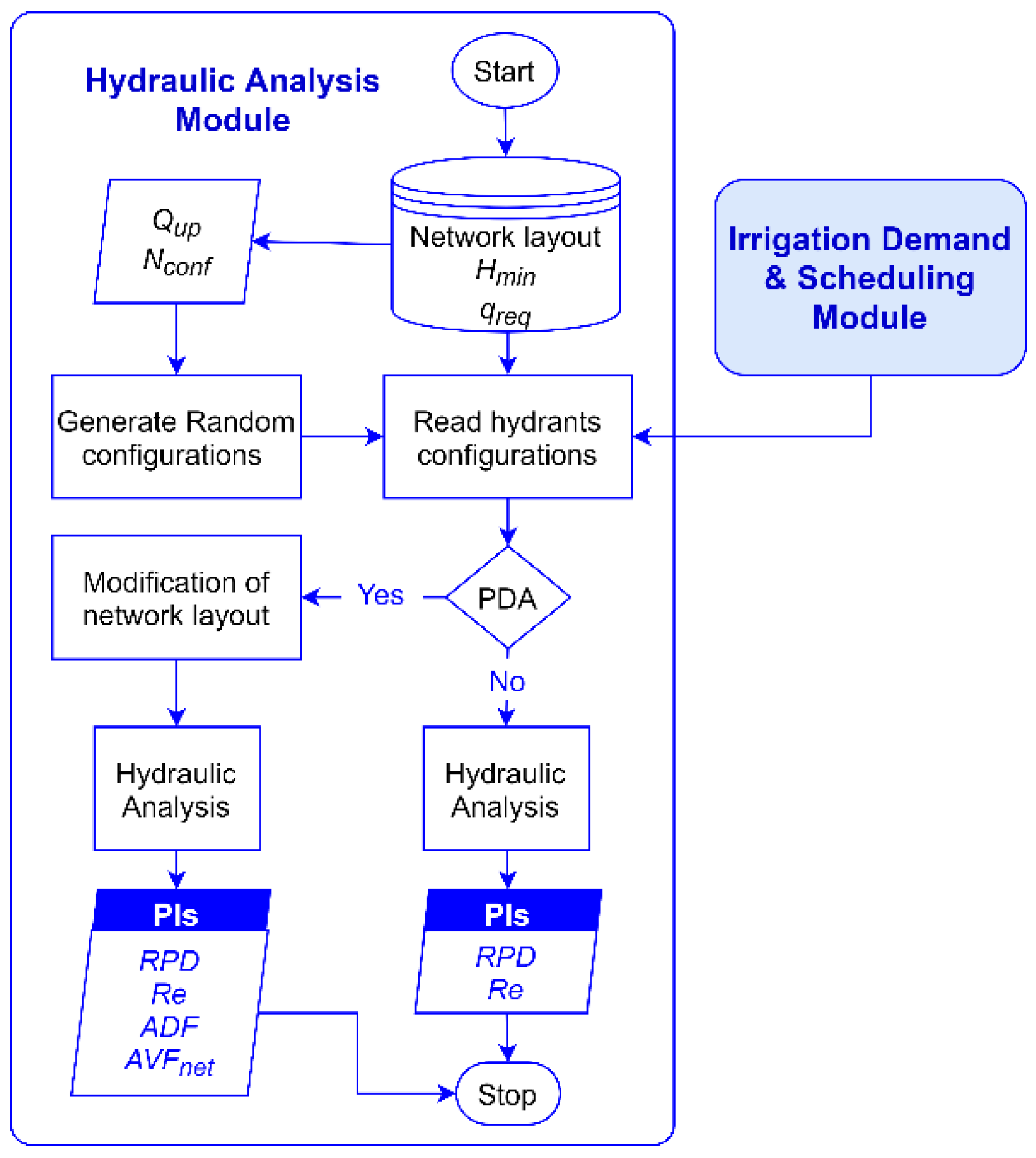
When the operating hydrant scenarios are available (defined by a certain number of configurations N_conf), the user of DESIDS can run either a DDA or PDA, according to the intended outcomes. For instance, if pressure at some hydrants falls below a minimum required level, the flow will be significantly reduced. In this case, PDA can be used to account for both pressure and demand deficiencies in the PIDS.

As mentioned above, the module uses an EPANET toolkit for the analysis process. This toolkit was selected because it is validated and extensively used in the hydraulic analyses of WDSs. Therefore, to avoid calling the toolkit in each analysed configuration, the module automatically generates the input file for EPANET by considering each configuration as a time step in an extended period simulation. The results of the analysis are then sorted and the generated PIs are presented in graphical and tabular forms to facilitate their interpretations. The process of the hydraulic analysis used in the module is presented in Figure 7.

2.3. Operation and Management Module

PIDSs are facing a mounting burden to provide solutions to the increasing water demand at the farm level. Therefore, the operation and management of these systems are crucial factors for achieving an efficient use of both the available water and the capacity of the systems to deliver the necessary pressures and demands to meet the requirements of on-farm systems and crops.

When designing PIDSs for on-demand delivery schedules, it is a common practice to calculate the probability of hydrants’ operation patterns using a method such as that proposed by Clément [15]. However, the foremost challenge in managing these systems in actual situations is to identify ahead of time the flows into the networks’ pipes, which are random and depend on the behaviour of farmers. In fact, even when the design flows are not exceeded, very low hydraulic performance can occur in these systems during their operation [35].

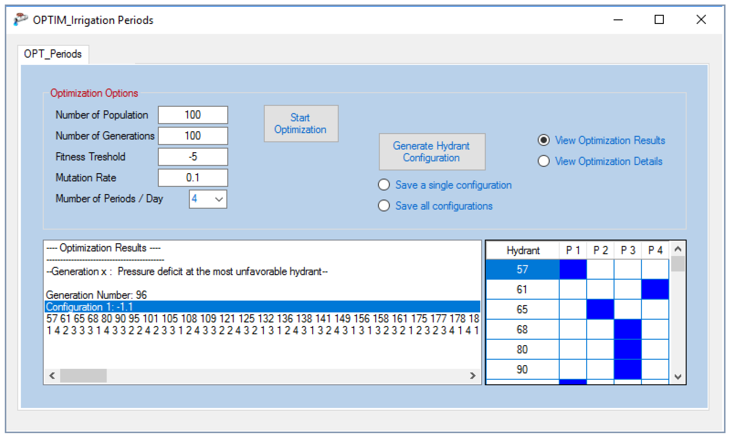
To this end, the aim of developing the operation and management module is to provide irrigation district managers with a useful tool which can be effectively used in finding solutions to PIDSs management under a wide range of scenarios. These solutions allow the improvement of the actual operation, as well as the sustainability of these systems. Accordingly, this module offers optimal management strategies for PIDSs designed for on-demand delivery schedule and facing performance problems, especially during peak irrigation demand periods, through the smooth transition to a rotation delivery schedule. The module uses the Genetic Algorithm (GA) for the optimization of irrigation periods, taking into account the minimization of the pressure deficit at the most unfavourable hydrant as its objective function (Figure 8).

2.3.1. Genetic Algorithms

GAs [38] are powerful metaheuristic search methods used for solving both constrained and unconstrained optimization problems, and are based on a natural selection process that mimics natural evolution. They use the same combination of selection, recombination and mutation to evolve a solution to a problem. These methods have been applied to the solution of many optimization problems in WDSs [39,40,41] because of the easy use of their properties and their robustness in finding good solutions to difficult problems.

GAs start with a randomly generated initial population, i.e., a set of solutions represented by chromosomes, which evolves through three main operators: (i) the selection, where chromosomes are selected from the population according to their fitness values to be parents; (ii) crossover, where some genes from parent chromosomes are selected to create new offspring. This is performed by randomly choosing one or more crossover point(s) where a pair of parent chromosomes exchange information; and (iii) mutation, which randomly changes the new offspring to retain the diversity of the solution in a population and expand the search in the solution space.

2.3.2. Optimization of Irrigation Periods

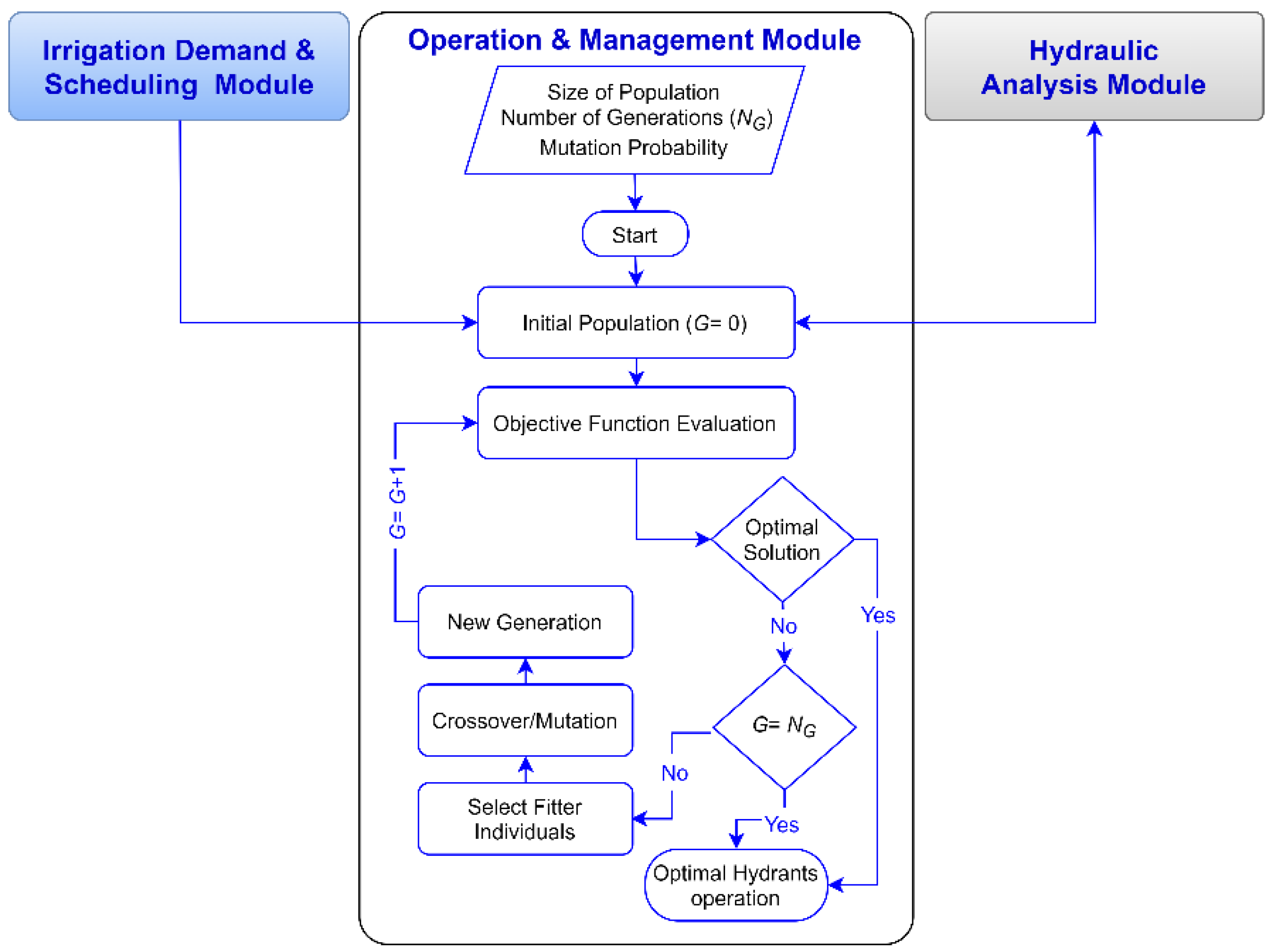
The main objective of this module is to offer irrigation district managers a tool to obtain the optimal operation of PIDSs when the latter are facing performance problems. The optimization process is carried out using GA. The module starts with a population of randomly generated individuals (chromosomes), each representing a possible solution that has to be evaluated by means of the considered objective function, which is the minimization of the pressure deficit at the most unfavourable hydrant in the network. The number of variables (genes) within the individuals is determined by the number of randomly generated open hydrants, while the values of these variables depend on the number of irrigation periods. In other words, each open hydrant is randomly assigned to an irrigation period. Therefore, the value of each variable ranges between one and the number of open hydrants.

The initial population is then evaluated by performing a hydraulic simulation, using the hydraulic analysis module, for each individual to obtain the pressure head of the open hydrants. The pressure deficit at the most unfavourable hydrant is then assigned to each individual and used as its fitness value. Based on their fitness, individuals with the lowest pressure head deficit (fitter solutions) are selected as parents and used to create new individuals (offspring) for the next generation. This is achieved through the processes of crossover and mutation. The crossover process implies that a pair of parent individuals exchange information in order to produce a pair of offspring that inherit their characteristics. Herein, this process is performed using a one-point crossover procedure, which entails that randomly selected pairs of parent individuals exchange information to produce offspring. The crossing point that cuts both parents at a point along the individuals is selected by randomly generating an integer number from one to the number of variables. The mutation process, on the other hand, alters one or more variable values in an individual from its initial state.

With every new generation, the above processes are repeated, and the algorithm stops either when an optimal solution has been reached or when the maximum number of generations has been achieved (Figure 9).

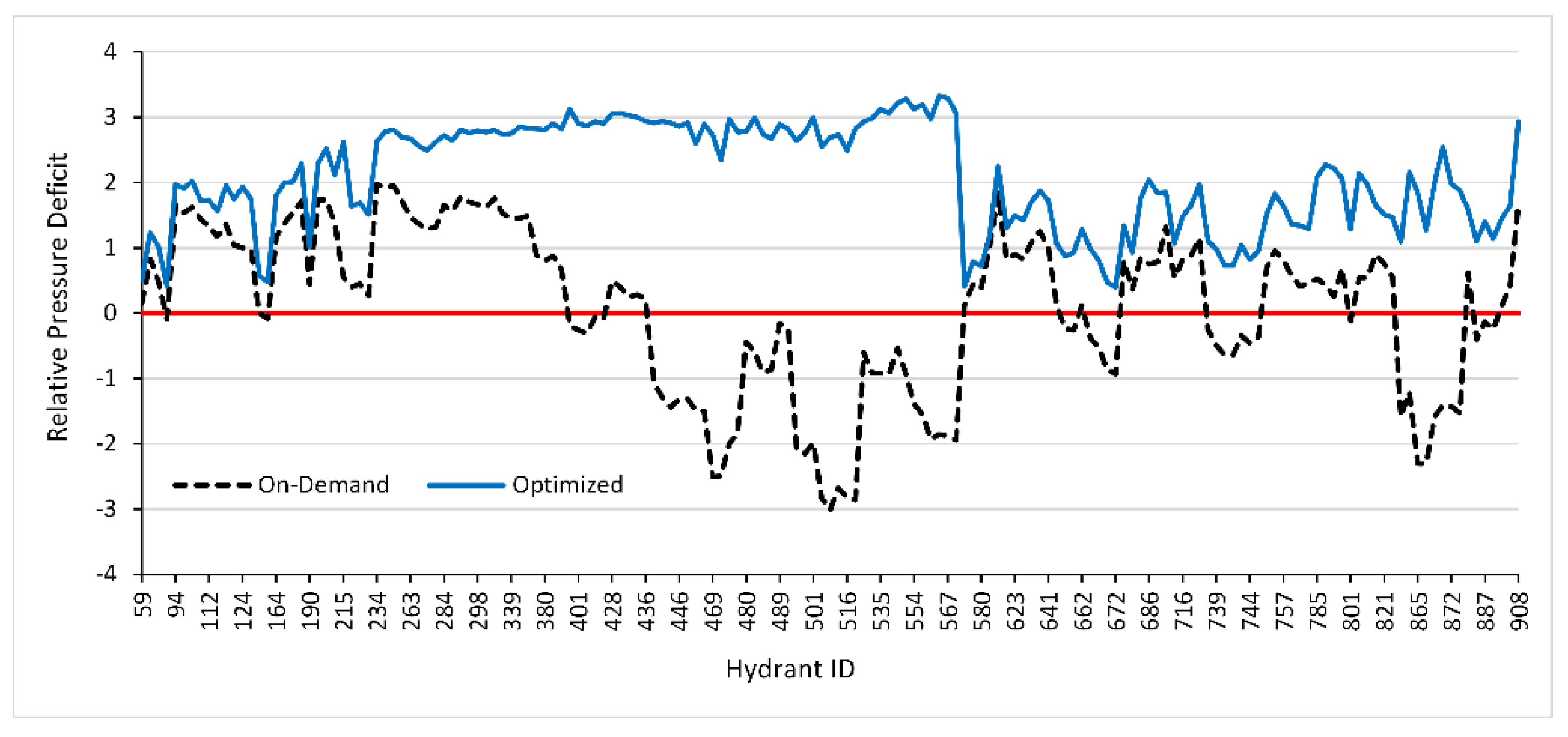
The operation and management module was tested on a large-scale irrigation distribution network operating on-demand, showing management solutions that successfully improve the hydraulic performance of the current failing conditions and ensuring the satisfaction of crop water requirements in all hydrants. These solutions were also able to overcome the significant increase in the upstream discharge of the tested PIDS, as reported in [42]. Figure 10 shows that, when the considered irrigation network was operating on-demand, around 42% of hydrants failed to provide the needed pressure, i.e., recorded pressure deficit. However, after the optimization of irrigation periods, using the operation and management module, all hydrants in this network recorded pressure higher than the minimum required for an optimal operation of on-farm irrigation systems.

2.4. Design and Rehabilitation Module

In some cases, improving the operation and management of PIDS alone does not cause a considerable improvement in networks’ hydraulic performances, unless combined with structural rehabilitation, especially if the systems’ performance failures are related to initial design flaws. This rehabilitation must ensure the minimum performance levels required to satisfy farmers while considering the associated cost over an extended period. Therefore, for a DSS to be complete, it is imperative to include a module for structural rehabilitation and design. To this end an effective tool for developing rehabilitation plans for existing PIDS or the design of new ones was incorporated into DESIDS. This module uses a non-dominated sorting genetic algorithm, NSGA II, for multi-objective optimization by considering the minimization of both pressure deficit at the most unfavourable hydrant and the rehabilitation cost. This algorithm was selected in this module for the optimization process because of its proven ability to efficiently search large decision spaces [43].

This module also considers the introduction of localized loops to existing networks’ layouts to increase their hydraulic capacity. This method was proposed by Lamaddalena et al. [44] and Fouial et al. [45], where it was tested on a real large-scale irrigation network and proved its ability to significantly improve the hydraulic performance of the network while providing considerable savings in the cost of rehabilitation. However, finding the position of loops was not automatic and was achieved through trial and error; thus, extensive and time-consuming data entries and analyses were required. In this module, an innovative algorithm was developed to automatically find the best looping locations in the network that can improve overall hydraulic performance.

This module was tested on a real case study in Southern Italy, as described in [46]. Two optimizations of an irrigation network rehabilitation were carried out. The first one included the option of adding loops by using the automatic looping operator, and the second one excluded that option. The obtained results clearly reveal that it is worthwhile to consider the localized loops option, as it provided considerable rehabilitation cost saving compared to the solution, which provided similar improvement but excluded the looping option (Figure 11).

2.4.1. The Non-Dominated Sorting Genetic Algorithm II

The NSGA-II [47] is one of the most popular Multi-objective evolutionary algorithms (MOEAs) used for the optimization of WDSs [43,48,49]. This is due to its efficient non-dominated sorting procedure and strong global elitism that preserves all elites from both the parent and child populations [50]. The objective of the NSGA II algorithm is to improve the adaptive fit of a population of candidate solutions to a Pareto front constrained by a set of objective functions. This algorithm uses an evolutionary process with surrogates for evolutionary operators, including selection, genetic crossover and genetic mutation. The population is sorted into a hierarchy of sub-populations based on the ordering of Pareto dominance. Similarity between members of each sub-group is evaluated on the Pareto front, and the resulting groups and similarity measures are used to promote a diverse front of non-dominated solutions.

2.4.2. Determination of Looping Positions

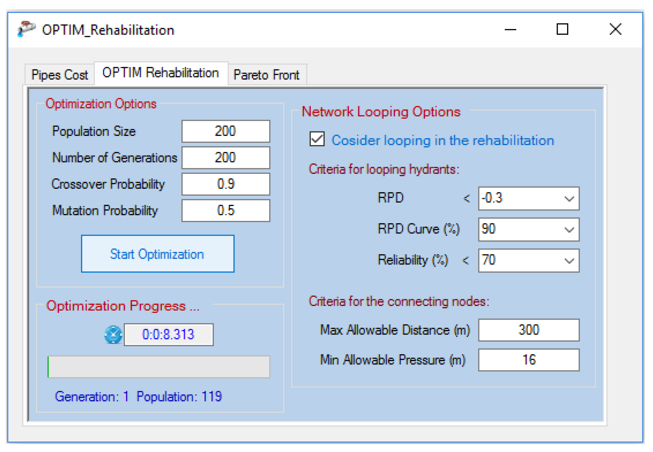
If the option of considering localized loops is selected, the algorithm is set to automatically search for the best looping positions by considering pre-defined conditions, as illustrated in Figure 10. These conditions are related to the initial hydraulic analysis results:

• A hydrant j is considered as a potential starting node for a loop l if its resulting RPD and reliability values are lower than the pre-defined limits.
• The RPD value of hydrant j belongs to the pre-defined RPD curve., i.e., the resulting RPDs from the initial performance analysis are organized into different RPD curves. The user of the module can select an RPD value for the considered hydrant from one of these curves, e.g., a 90% curve.
• A node nd (can be a connecting node or hydrant) is considered as a potential ending node for the loop l (starting from hydrant j) if its distance from hydrant j is smaller than the pre-defined maximum allowable distance. The distance is calculated from the X and Y coordinates of hydrant j and node nd using:

  Distance = sqrt((X_nd − X_j)² − (Y_nd − Y_j)²)

  (13)
• The node nd is considered if its pressure head is higher than the minimum allowable limit.

The abovementioned conditions are set to (i) position the localized loops only when needed to improve the hydraulic performance and (ii) limit the number of suggested loops to increase the efficiency of the algorithm during optimization. Figure 12 shows the looping conditions when looping is considered in the optimization of a PIDS rehabilitation. Each of the selected hydrants in this process is compared to all nodes in the PIDS. If all the above conditions are met, the looping pipes are added to the original layout database, with a respective length, initial and final nodes and an initial pipe diameter value of 0.

2.4.3. The Multi-Objective Optimization of PIDS

The design and optimization module was developed primarily for the rehabilitation of existing PIDSs. If this is the objective of the decision maker using this module, then the layout of the network to be rehabilitated is considered as known and all pipes in this case are predetermined based on the positions of existing pipes. The PIDSs rehabilitation is formulated as a bi-objective optimization problem, with a selection of pipe diameters as the decision variables. The decision variables (pipes to be sized) and allowable selections for each decision variable (available pipe diameters and permissible range of pipe diameters for each section of the network) are identified. The developed algorithm is set in a way that some constraints are addressed at the beginning of the optimization procedure. First, considering the range of pipe diameters, available diameters for a specific section in the network are constrained to an upper and lower bound, with the latter being the existing pipe diameter of the same section. In other words, the algorithm considers only a diameter that is equal or larger than the existing one. In the case where the design of a new network is considered, the initial pipes’ size can be set to zero, which will be the lower bound for all pipes. Second, the algorithm ensures that all the solutions in the search space will respect the constraints that the pipe diameters of the upstream pipes are larger than those of the downstream ones.

The multi-objective optimization of PIDS rehabilitation is used to explore the trade-off between the two considered objective functions, formulated mathematically as:

An objective function of pressure deficit minimization (OFPD), described as:

OFPD = H_j,min − H_j

(14)

where H_j,min is the minimum pressure head required at hydrant j (m) and H_j is the actual pressure head at hydrant j (m). Both values are related to the most unfavourable hydrant in the network. Thus, a positive value of the OFPD indicates the highest available pressure deficit in the network, while a negative value indicates the lowest pressure surplus. This formulation provides a wider range of solutions, and therefore a better comparison between the cost of allowing some deficits in the network (that do not affect farmers) and a pressure surplus.

An objective function of minimization of the total cost of rehabilitation (OFCR), described as:

OFCR = ∑^Nk C_k L_k

(15)

where k is the pipe index, N_k is the total number of pipes in the network including the suggested loops, C_k is the unit cost associated with commercially available pipe diameter D_k (€m⁻¹) and L_k is the length of pipe k (m). OFCR is formulated to be used for both the design of a new network and the rehabilitation of an existing one. In the latter case, only the cost of the replaced pipes is considered. Thus, the cost, C_k, of the remaining pipes is set to 0.

Then, the developed algorithm in the design and rehabilitation module (Figure 13) starts by generating a random initial population (individuals), respecting the abovementioned pipe constraints. Each individual is then assigned a value for each objective function (cost and pressure deficit). It is worth mentioning that the evaluation of individuals is obtained under an extended period simulation mode, i.e., using the same hydrant configurations used in the initial hydraulic analysis of the existing network. The individuals are then sorted into fronts in a way that the solutions of the first front are not dominated by any other solutions in the population. Then, solutions of the second front are only dominated by solutions of the first front, etc. Next, the solutions within each front are assigned a crowding distance, which gives a measure of how dense the front is in the vicinity of that solution [47]. Subsequently, an offspring population is created by selecting individuals of the current population and performing the operations of crossover and mutation (respecting pipe constraints) to produce new solutions. When selecting solutions, individuals are compared by their front numbers, giving preference to the lower numbered fronts. If two solutions are from the same front, then the solution with the greater crowding distance is chosen [51]. These processes are repeated until a maximum number of generations has been reached.

3. Conclusions

An integrated DSS, called DESIDS, was developed. The DSS, which encompasses four different modules, is an innovative tool to help irrigation district managers and decision makers in addressing the key issues and challenges often found in PIDSs, including planning, analysis, operation and rehabilitation processes. The four discrete modules were developed in a decoupled fashion to maximize their use in the previously mentioned processes and to support future expansions and integrations in DESIDS. These modules were tested in various case study applications to explore different operation and management options available to irrigation managers and decision makers. It is evident that DESIDS is a useful technical tool which can provide objective information to inform decision making in actual and future decisions related to PIDSs. The developed DSS can be used as a platform for future integrations and expansions to include other processes needed for better decision-making support. For instance, DESIDS does not analyse energy consumption and does not consider energy consumption in the optimization processes. Future integrations of this DSS should include these options to explore energy savings in the decision-making process.