Experimental Validation of an Innovative Approach for GDI Spray Pattern Recognition

1
Loccioni, 60030 Angeli di Rosora, Italy
2
Department of Engineering, University of Perugia, 06125 Perugia, Italy
*
Author to whom correspondence should be addressed.
Fuels 2021, 2(1), 16-36; https://0-doi-org.brum.beds.ac.uk/10.3390/fuels2010002
Submission received: 30 November 2020
/
Revised: 29 December 2020
/
Accepted: 8 January 2021
/
Published: 21 January 2021
Abstract
:In the present automotive scenario, along with hybridization, GDI technology is progressively spreading in order to improve the powertrain thermal efficiency. In order to properly match the fuel spray development with the combustion chamber design, using robust and accurate diagnostics is required. In particular, for the evaluation of the injection quality in terms of spray shape, vision tests are crucial for GDI injection systems. By vision tests, parameters such as spray tip penetration and cone angles can be measured, as the operating conditions in terms of mainly injection pressure, injection strategy, and chamber counter-pressure are varied. Provided that a complete experimental spray characterization requires the acquisition of several thousand spray images, an automated methodology for analyzing spray images objectively and automatically is mandatory. A decisive step in a spray image analysis procedure is binarization, i.e., the extraction of the spray structure from the background. Binarization is particularly challenging for GDI sprays, given their lower compactness with respect to diesel sprays. In the present paper, two of the most diffused automated binarization algorithms, namely the Otsu and Yen methods, are comparatively validated with an innovative approach derived from the Triangle method—the Last Minimum Criterion—for the analysis of high-pressure GDI sprays. GDI spray images acquired with three injection pressure levels (up to 600 bar) and two different optical setups (backlight and front illumination) were used to validate the considered algorithms in challenging conditions, obtaining encouraging results in terms of accuracy and robustness for the proposed approach.
1. Introduction
In last years, environmental issues have become the effective driving force for automotive powertrain technical evolution. Both toxic and CO2 emissions are regulated by stringent legislations implying the adoption of severe limits applied over highly transient laboratory and real-driving test cycles. In order to comply with these severe constraints, the automotive industry is progressively introducing hybridization technologies, along with advanced combustion and after-treatment systems.
For spark-ignited engines, a significant thermal efficiency improvement is allowed by the shift from homogeneous charge combustion (typical of PFI engines) to stratified charge combustion enabled by fuel direct injection technology (GDI engines). The efficiency improvement potential is mainly related to the mixture quality-control approach, which is enabled by stratified charge combustion, particularly for low and medium speed and load operating conditions.
The attainment of the efficiency potential offered by GDI technology implies an accurate control of the air–fuel mixture formation process, which in turn deeply affects both combustion and pollutants formation, basically NOx and particulate. In GDI engines, mixture preparation is determined by the interaction among fuel sprays and surrounding air, resulting in severe requirements in terms of fuel metering accuracy, injection rate control, fuel atomization level, and sprays targeting and evolution.
In this scenario, the development of robust methodologies to verify the actual behavior of high-pressure gasoline injection systems is crucial for the automotive industry. In particular, in order to correctly match the injection system operation with a specific combustion chamber, the spray global evolution is to be precisely determined as a function of time in a large range of operating conditions. Testing parameters often include the injection pressure level, fuel temperature, and downstream temperature and pressure.
The fuel jet’s global evolution is conventionally described in terms of a number of parameters such as the spray tip penetration, single spray diffusion angle, bend angle among jets, and spray boundary area. The measurement of these quantities is obtained by the analysis of spray images acquired using different optical arrangements. Given the relevant number of operating parameters and the need for a statistically significant base for each operating condition, the acquisition and analysis of several thousand images is typically required to obtain an adequate knowledge of the spray evolution. As a matter of fact, the adoption of an automated (on-line or off-line) image analysis procedure is mandatory in order to speed up the test methodology while preserving its objectiveness and accuracy in the spray parameters detection.
The aim of this paper is evaluating the efficacy of different automated spray analysis methodologies applied to the study of GDI sprays. In this study, in addition to the analysis of existing and widely adopted approaches, a new algorithm is introduced and validated. The validation study of the considered spray analysis algorithms is carried out using an experimental image database relevant to GDI sprays obtained with three injection pressure levels: 200, 400, and 600 bar. In particular, the use of a significantly high injection pressure level extends the present validation significance, including operating conditions that are likely to be adopted by the automotive industry in the near future.
2. Imaging Analysis of GDI Sprays
Generally, the first and crucial step in the image analysis procedure is recognizing the spray from the background, thus defining its boundary. From the resulting spray boundary, the global geometrical characteristics of the spray at the considered timing will be determined. In general, if a camera acquires images with a bit depth of n, every pixel in the image is associated with a light-intensity level defined according a 2n gray rule. Considering a typical spray image frequency histogram (Figure 1, backlight spray image), extracting the spray from the background means selecting a gray level located between the two frequency local peaks belonging to the spray and to the background, respectively. This gray level will be assumed as a threshold among pixels with a low gray level pertaining to the spray, and pixels with a high gray level were assumed as part of the background.
The appropriate gray-level threshold can be suggested by the experience of the operator, but the human perception in setting the threshold can significantly influence penetration and angles calculation. As a consequence, in many automated spray image analysis procedures, dedicated algorithms are used to automatically determine the gray-level threshold associated with the spray boundary. In general, developing an efficient automated spray boundary detection procedure ensures the analysis stability over large databases and the reproducibility of the analysis. Furthermore, the comparison among different databases is enabled, even if experimental data are acquired with different optical approaches.
The accuracy of the image analysis algorithm is significantly influenced by the image contrast or signal-to-noise ratio. This quality of spray images depends on the illumination system, on the local density of the injected fluid, and on the spatial distribution of the spray drops with respect to the camera focus plane. As a consequence, the spray image quality in terms of light contrast is influenced basically by the injection pressure and by the delay between the injection process start and the timing of image acquisition, both these parameters affecting the image signal-to-noise ratio. Furthermore, both the fuel and the ambient temperature can have a significant effect on the spray droplets space density. As during a generic spray experimental campaign, the images signal-to-noise ratio cannot be kept constant, an automated image analysis algorithm that is able to recognize the spray with different image contrast levels is mandatory. In fact, the algorithm must efficiently recognize the spray from the background in a range of different test conditions, mainly in terms of injection pressure, at different timings from the injection start beyond the injection end, when the spray density is significantly reduced.
The image analysis can follow two different approaches in terms of spray boundary recognition: the spray edge detection can be based on the first or second local derivate of the light intensity function, or it can be based on a threshold level selection that is globally able to differentiate the spray from the background pixels.
According the first approach, methodologies can be used similar to the one proposed by Canny et al. [1] or by Klein-Douwel et al. [2] to recognize the spray edge by analyzing local steep changes of gray level of the pixels. These approaches are typically very sensitive to local brightness variations and so they can detect any local change of pixel values: among these local boundaries, the external edge is not clearly highlighted. In some algorithms following the local light gradient approach, the test operator can select some parameters to better detect the external spray edge, but this introduces a factor of subjectivity in the spray pattern recognition procedure. As a matter of fact, in order to obtain a satisfactory efficacy, these methodologies generally need some adaptation to the injection system type (e.g., diesel or GDI) and operating conditions in terms of injection pressure, test vessel density and temperature, stage of spray development.
The second spray detection approach is based on methods that select a global threshold according to the statistical distribution of gray-level values in the image. Some of these methodologies, such Niblack’s method [3], divide the image into a certain number of windows and select one specific threshold for each window. The subdivision of the image into windows is performed by the operator; if the image partitioning is different, the global result can be different. Other methodologies consider the histogram of the whole image and select a single threshold, such as the approaches proposed by Otsu et al. [4], Yen et al. [5], Naber et al. [6], and the so-called Triangle Method [7]. Methodologies pertaining to this last group are supposed to be able to apply an automated and objective strategy to analyze images.
In the present paper, an innovative spray image analysis approach is proposed, which is named as Last Minimum Criterion (LMC in the following) and derived from the Triangle Method. In order to verify the proposed approach efficacy, the Otsu, the Yen, and the LMC methodologies are comparatively applied for the analysis of a GDI spray evolution so to evaluate the difference in terms of spray tip penetration and spray angles. Furthermore, the same spray image dataset was analyzed by means of a constant-threshold level approach, which was specifically optimized for a given operating condition and applied for all the image acquisition timings. In order to further extend the validation significance, two different sets of spray images were used, which were respectively acquired with two optical setups: backlight and front light. In the first case, the injector is placed between an illumination source and a CCD camera; the shadow of the spray on the lit background is acquired. In the second case, a diffuse illumination field is created, and so the light scattered from the spray drops is acquired by the camera, resulting in a dark background.
2.1. Theoretical Background
The final aim of the considered spray analysis methodologies is developing a self-adaptive and objective procedure for the extraction of the spray contour from the background. The spray boundary recognition is based on the computation of a gray-level threshold to separate pixels pertaining to the spray from background pixels. The developed procedure should be efficient for the analysis of images acquired using both a backlight and a front-light optical setup. The Otsu, Yen, and LMC methods are presented below.
2.1.1. Otsu Method
This method analyzes the histogram of gray levels for the pixels of the whole image and selects a global threshold. An image (black and white images are considered) is composed by N pixels, each being characterized by a gray level ranging from 0 to L. In the image gray-level histogram, for each level i, a number of pixels nj is represented. The gray-level histogram is normalized, and so the parameter density of probability p is defined as below:
Gray levels can be separated into two groups or classes G0 e G1 by a generic gray level h:
Now, the global probability to have a pixel in one of these classes is
The total mean gray level of the whole image is
This mean gray value can be calculated for each class:
From Equation (5), the total mean gray level is
The classes variance can be defined as:
Following from Equations (6) and (7), the within-class variance is
and the between-class variance is
The total variance of levels is
According to the Otsu methodology, the best threshold is the gray level yielding the best separation of classes in gray levels. In this way, the optimal threshold maximizes .
2.1.2. Yen Method
For a given gray level h, the probability of the gray level is normalized, and two distributions can be defined as:
where .
This method, which is also called Maximum Correlation Criterion, uses the function of correlation. Considering a variable y and its probability , the correlation function is defined as:
Related to the two classes and , and are defined as below:
The total amount of correlation is
The Yen method defines the optimal threshold as the level which maximizes the total correlation:
2.1.3. Last Minimum Criterion
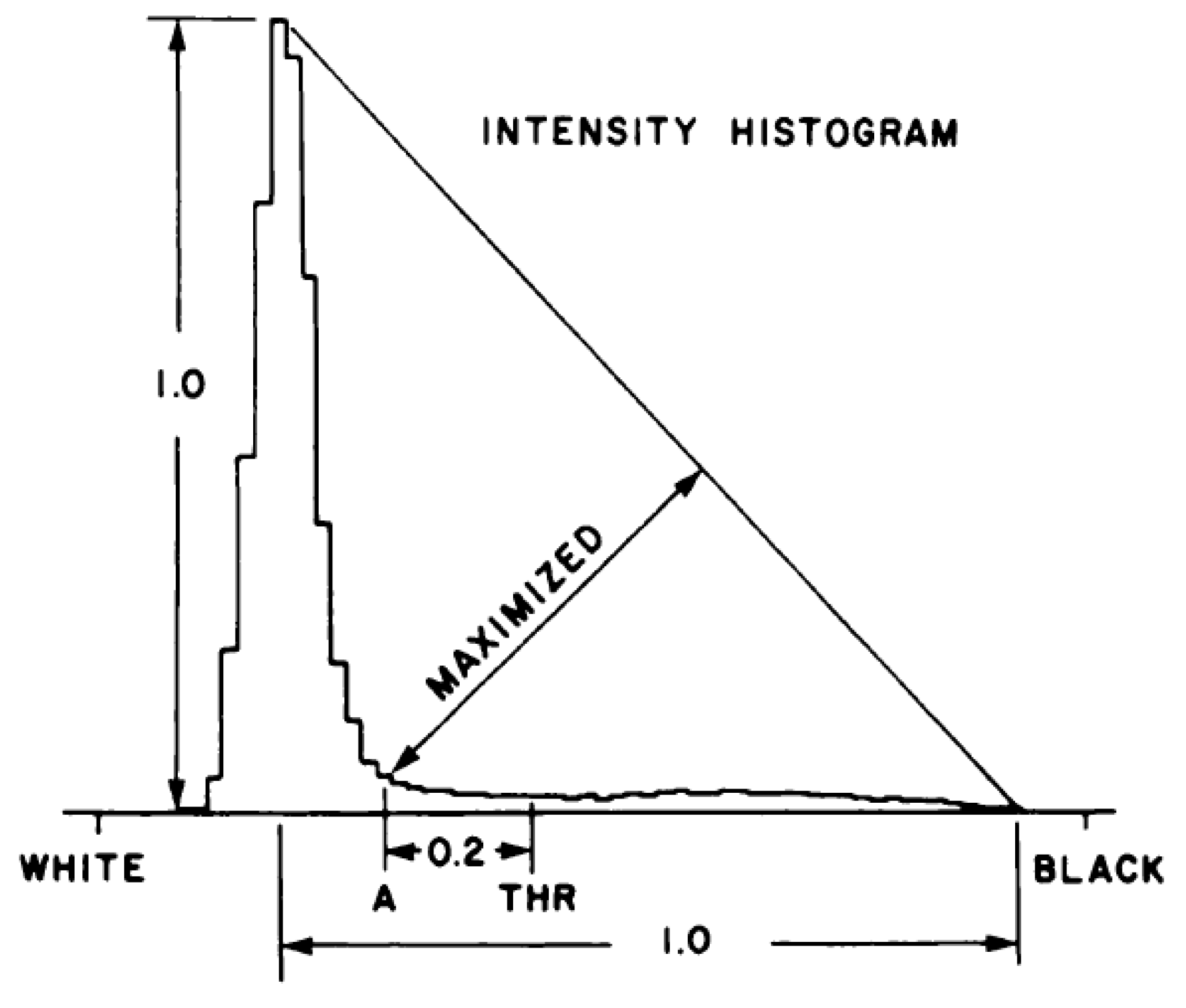
The Triangle method was developed in 1977 by Zack et al. [7] for the automated recognition of human metaphase chromosomes from a bright background. According to this method, the image of the gray-levels histogram is normalized, and a line is drawn from its peak to the highest value of the histogram (Figure 2). The maximum distance between the drawn line and the histogram curve detects a gray level, which was added to a fixed offset (0.2) to obtain the threshold. This method is effective when the background is evidently dominant with respect to the searched object.
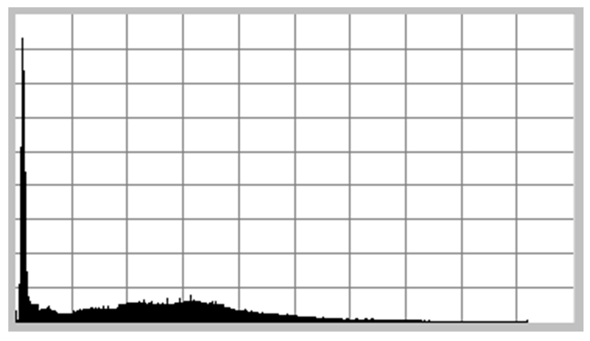
In a typical spray image, two peaks are present, which represent the background and the spray, respectively. Normally, a very high frequency peak is relevant to gray levels from the background pixels, while the lower peak represents the spray structure. Unfortunately, the typical shape of pixel values frequency distribution for a spray image changes with the acquisition timing. At the beginning of the injection process, the spray structure is very dense, and the spray pixels are very bright (or dark for backlight imaging), but the number of pixels that represent the spray is very low with respect to background pixels. Conversely, when an image is acquired with a high delay from the start of injection, the number of spray pixels is higher, but its pixel values are distributed over a wide range of gray levels, and the corresponding peak is smoothed (Figure 3).
In both cases, the zone of the frequency distribution representing the background is characterized by one or more local maxima that are significantly higher than the spray peak. Unfortunately, the original Triangle Method is not appropriate for the analysis of GDI sprays, because here, the threshold is calculated considering the absolute maximum of the frequency distribution peak, which is not relevant to the spray.
In order to correctly identify the valley between the background and the spray in the image histogram, the background local maximum nearest to the spray has to be considered.
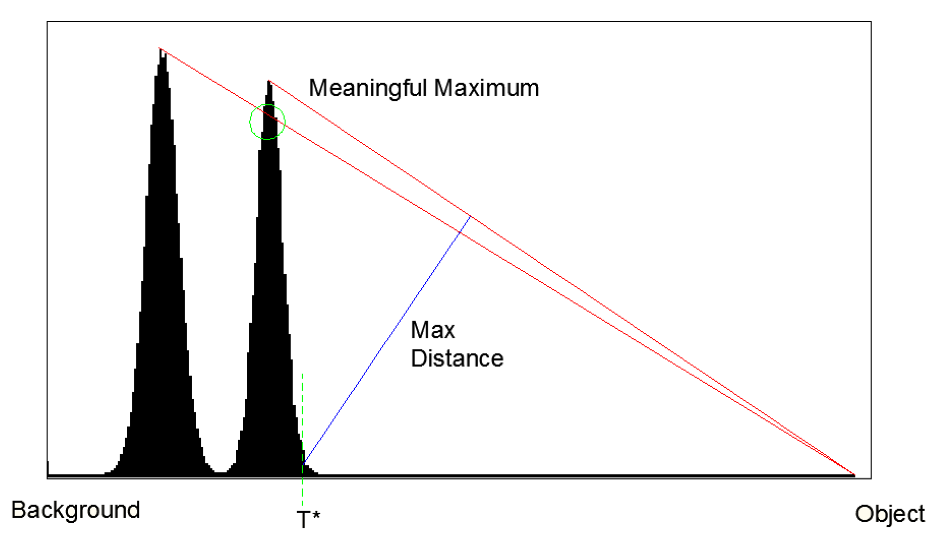
In order to attain this goal, the concept of the Last Minimum is introduced. The absolute maximum of the image histogram is considered; a line between this point and the last value of the histogram relevant to the spray (black in the backlight configuration and white in front-light configuration) is drawn. The Triangle Rule is applied, and a gray level T is calculated. If this line is external (not crossing) or it is tangent to the histogram curve, the computed T value is assumed as the searched threshold T*.
Conversely, if the line cuts the histogram, the sub-histogram between the following maximum and the last gray level relevant to the spray is considered. The above described procedure is repeated for this part of the histogram, verifying that the new connecting line is external or tangent to the histogram (Figure 4). When this condition is met, the gray level of the histogram which is at the maximum distance from the last line drawn is the searched threshold value T*.
Differently from the original Triangle Method, this approach does not need an offset (0.2 in Figure 2) to correct the threshold, and hence, it is totally automatic.
2.2. Experimental Setup and Test Plan
In order to compare the Otsu and Yen methods and to validate the proposed LMC approach when applied to the automated analysis of GDI sprays, a dedicated experimental campaign was carried out. In the following, details of the experimental setup and test plan are reported.
2.2.1. Image Acquisition
Images are acquired according to an ensemble-average approach, capturing one frame per injection event at a given delay from the process trigger, which is assumed as the start of the logic command for the injector driver. This way, a group of frames (30 in the current campaign) is collected for each considered timing in order to have a statistically significant basis to account for the spray evolution shot-to-shot dispersion.
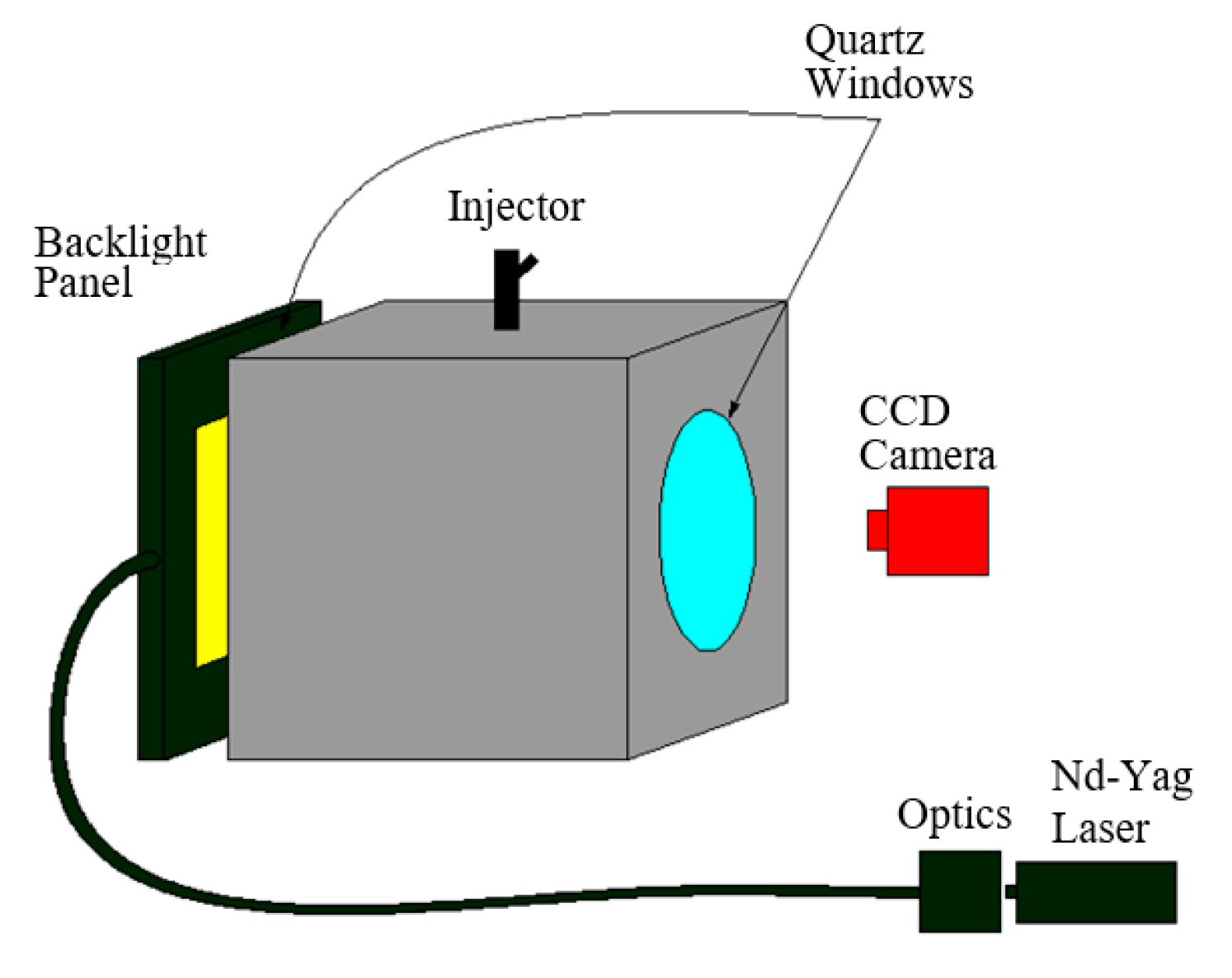
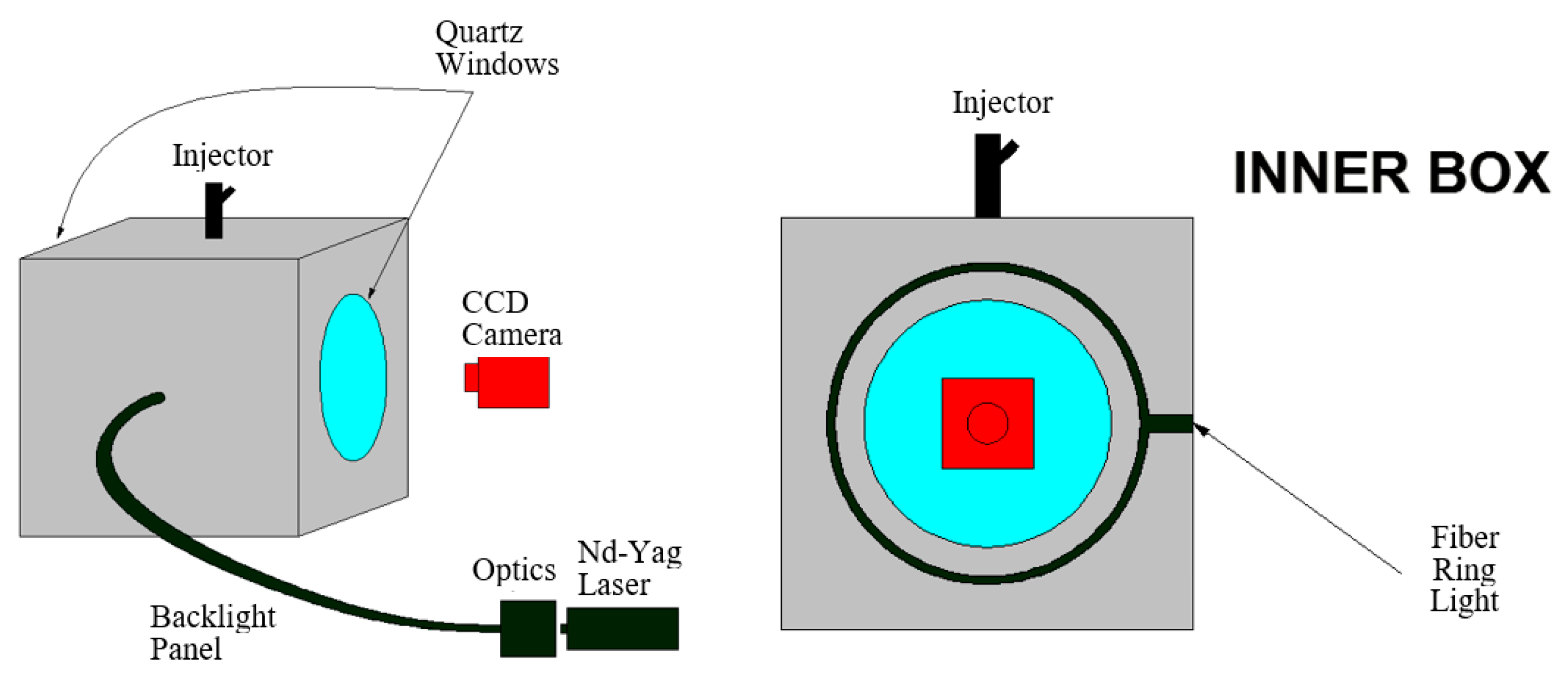
The imaging system is based on a Sensicam CCD camera by PCO (12 bit, 1376 × 1040 res, 1 µs min acquisition time, 15 fps at full frame) synchronized with a pulsed Nd-Yag Laser (New Wave Research Solo-PIV, 532 nm, 50 mJ/pulse, 10 ns pulse duration, max repetition rate 20 Hz) as a light source. The extremely short pulse duration determines the actual exposure time, significantly reducing the image blur. Two different optical arrangements were used in order to better evaluate the behavior of each analysis method: backlight (BL) and front-light (FL) configuration, respectively (Figure 5 and Figure 6). In the backlight arrangement, the injector is placed between a lighting panel and the CCD camera, while an optical fiber drives the laser light into the backlight panel. Accordingly, the camera acquires the shadow of the evolving spray, resulting in dark-on-bright images. In the front-light system, an optical fiber ring light is used to illuminate the spray from the same side and co-axially with the CCD camera. As a result, the light scattered by the spray drops is collected obtaining bright-on-dark images.
The injector is vertically positioned on the top of a closed test vessel, which is designed to operate up to 12 bar. The test vessel is equipped with circular optical accesses (100 mm diameter) respectively for illumination and image acquisition. The injector actuation frequency is limited to typically 2–4 Hz by the need to evacuate the previously injected fuel fog from the test vessel, in order to preserve the image quality. Accumulated fog in the test chamber causes noise in the acquired images (background is no longer uniformly dark or bright, depending on the optical arrangement), which tends to corrupt the information in the new injection event image.
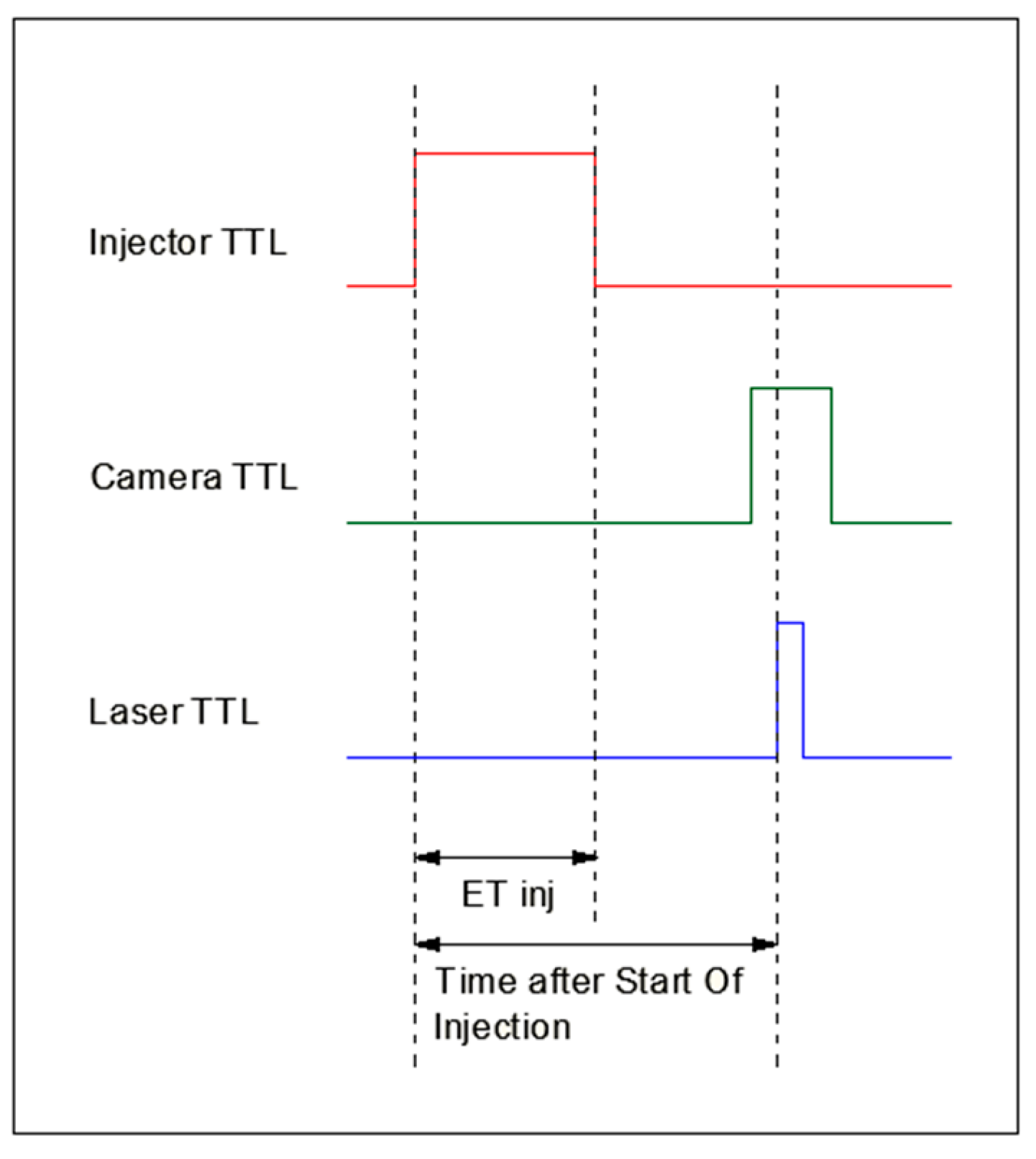
Synchronization between the injector, light system, and CCD camera is controlled by an NI PCIe-6231 board and follows the logic reported in Figure 7. The injection logic command (TTL) is sent to the injector driver, with the injector Energizing Time corresponding to the TTL time length. The camera TTL rising edge drives the CCD shutter aperture, with a nominal exposure time of 10 µs. During the CCD exposure period, the laser Q-switch is activated by the laser TTL signal, and the laser light pulse is emitted for 10 ns, defining the actual spray image acquisition timing (time after the start of the injection process) and image exposure. Globally, a 1 µs time resolution is attained by the synchronization system. Further details about the experimental setup used for the present tests are reported in [8,9,10].
The injector (Magneti Marelli IHP600) is driven by an AEA 170.1 programmable peak-and-hold driver. The operating parameters are described in Table 1.
2.2.2. Test Conditions
The energizing time of the injector was set to 1500 µs for the entire experimental campaign, while the test vessel pressure and temperature were maintained at room conditions (1 bar and 20 °C). In order to evaluate the actual performances of the examined image analysis approaches, different injection pressure levels were tested: 200, 400, and 600 bar. Both backlight and front-light optical arrangements were used. With the aim of acquiring the whole injection phenomenon, 26 acquisition timings after the Start of Injection (SOI) were explored, with 30 images acquired per timing.
2.2.3. Image Analysis Procedure
Each acquired image was analyzed by a completely automated routine developed in the LabVIEW Vision environment to evaluate the average value and the standard deviation of the spray tip penetration and cone angles.
The automated image analysis software is composed by four logic parts: image pre-conditioning, binarization, edge extraction, and spray parameters calculation.
The pre-conditioning step performs a background subtraction and a Region-of-Interest (ROI) application. A separately acquired background image is subtracted from the spray image in order to eliminate flaws in the background and to clearly highlight the spray. In detail, this analysis step is mandatory for images acquired by the backlight optical setup, as they are particularly sensitive to background defects that could alter the apparent spray structure.
In order to evaluate the gray-level threshold corresponding to the spray boundary, the area that potentially can be occupied by the spray is considered. In the present analysis, a circular ROI was used to follow the shape of the test vessel windows. The windows border was excluded from the ROI to obtain a perfectly even background, while a part of the injector tip and all “spray area” were comprised in the used ROI. The same circular ROI was used for both the backlight and front-light configurations.
After the pre-conditioning step, the image was binarized according to Otsu, Yen, and LMC approaches. The threshold value was applied on the image and the spray contour was extracted. Basing on SAEj2715 rule [11], the spray tip penetration and spray cone angle were calculated.
3. Results and Discussion
In order to visualize the capability of the adopted automated methodologies in locating the spray boundary, in the following, some of the obtained results are reported.
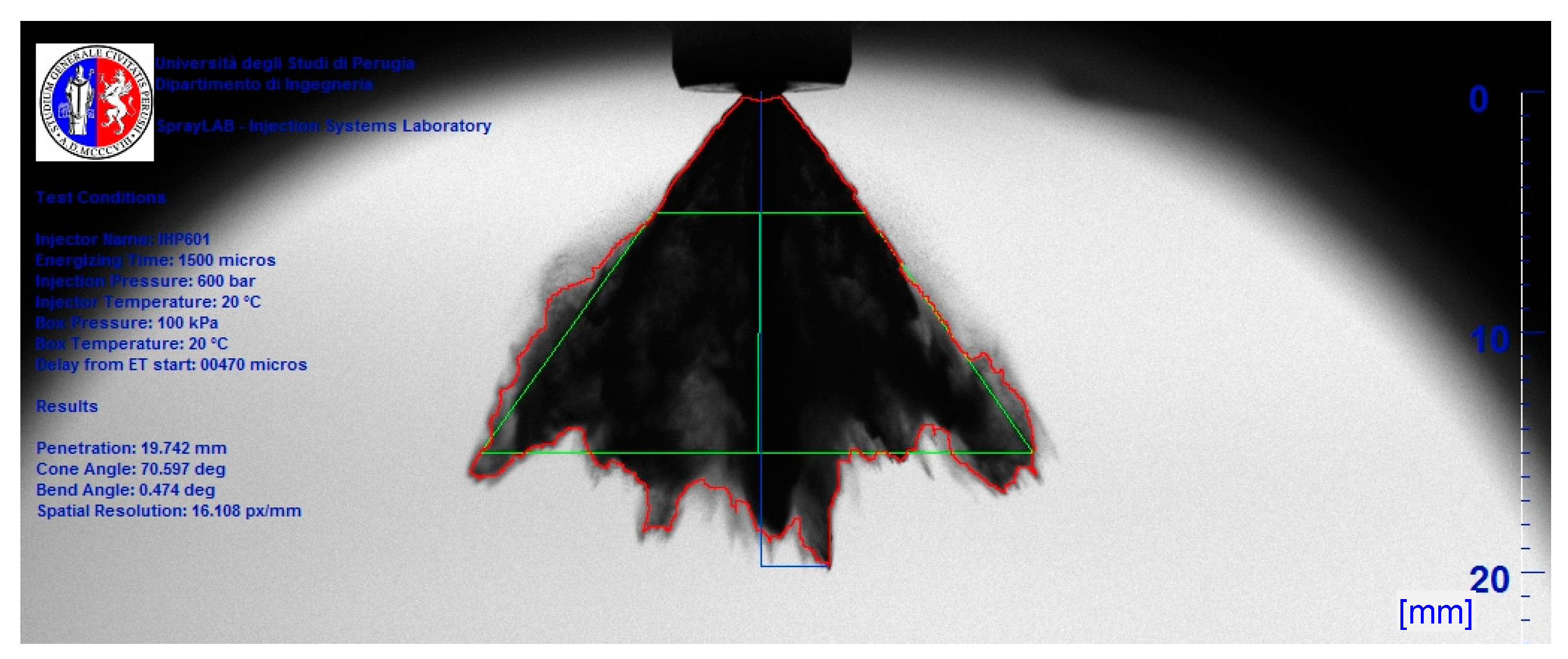
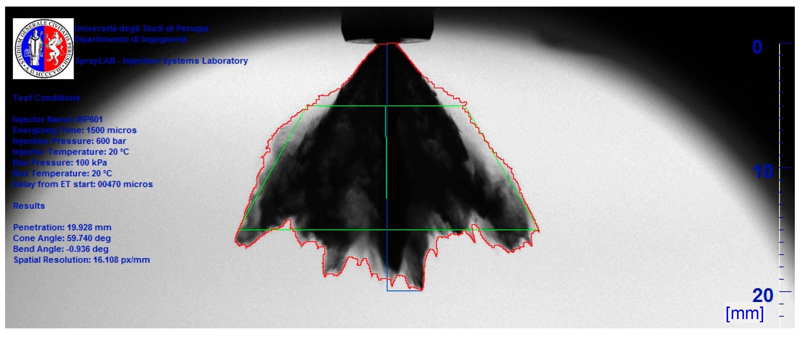
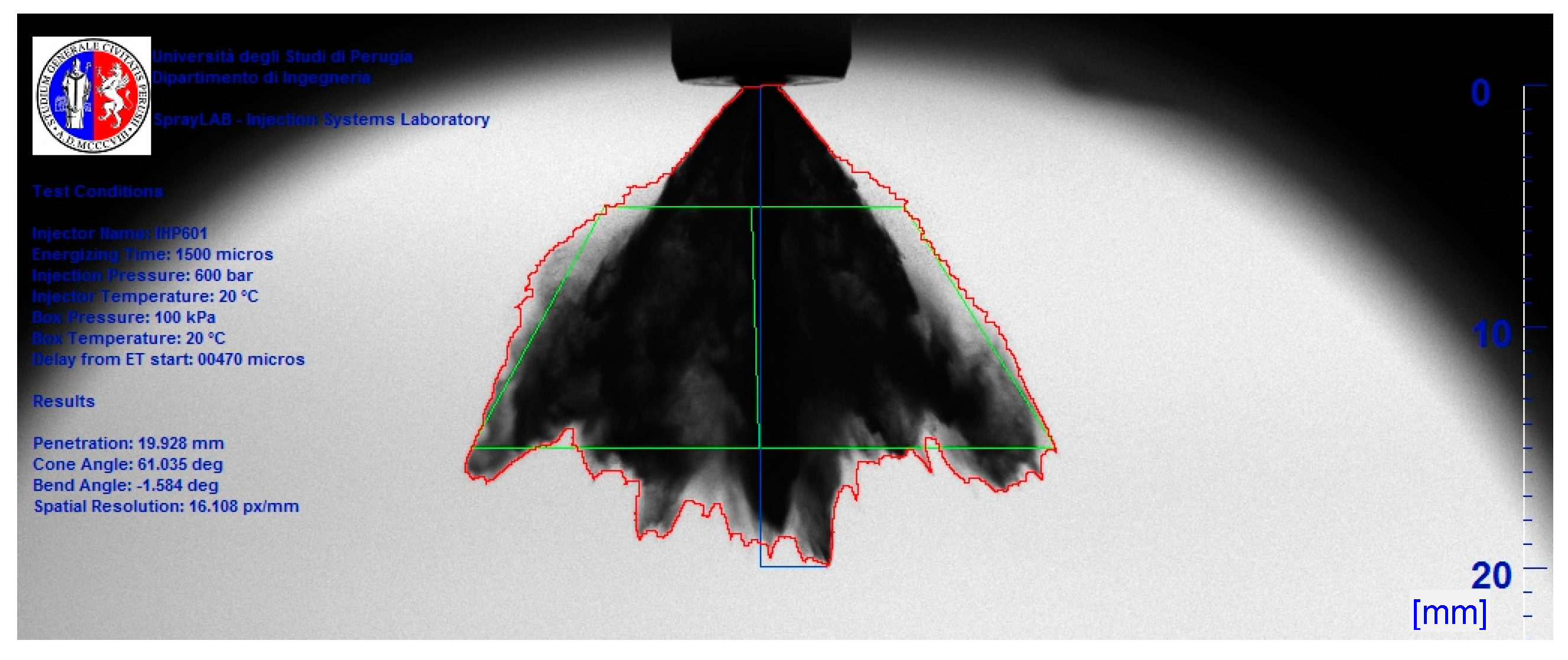
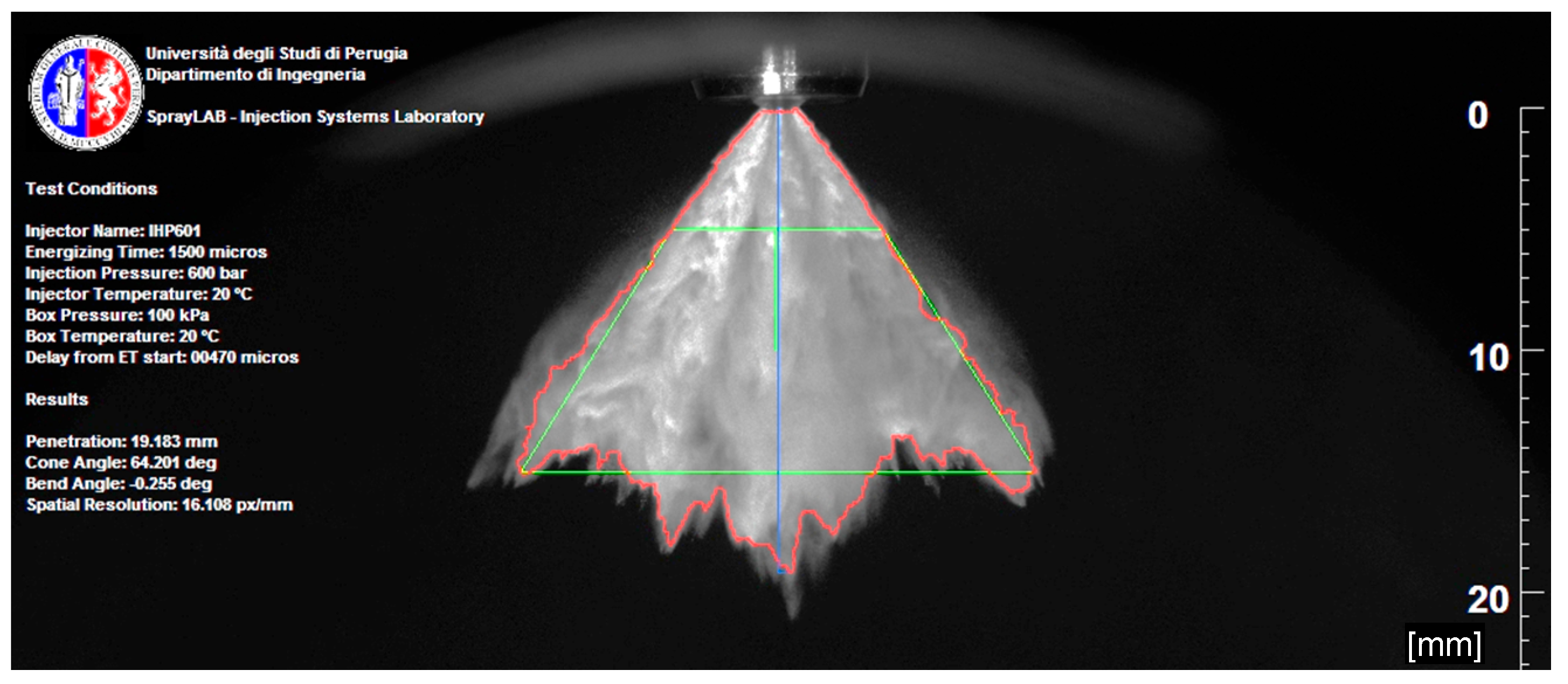
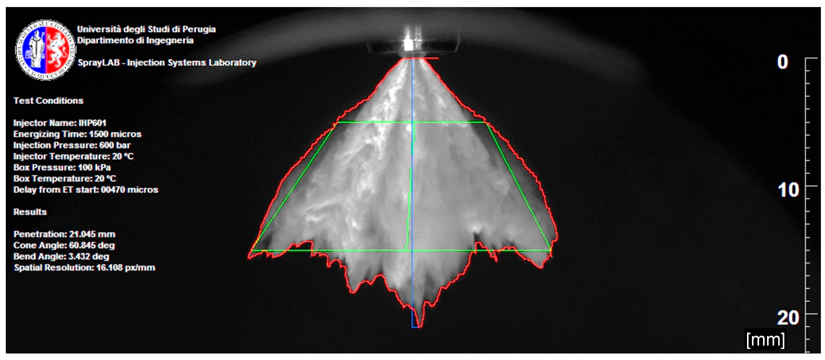
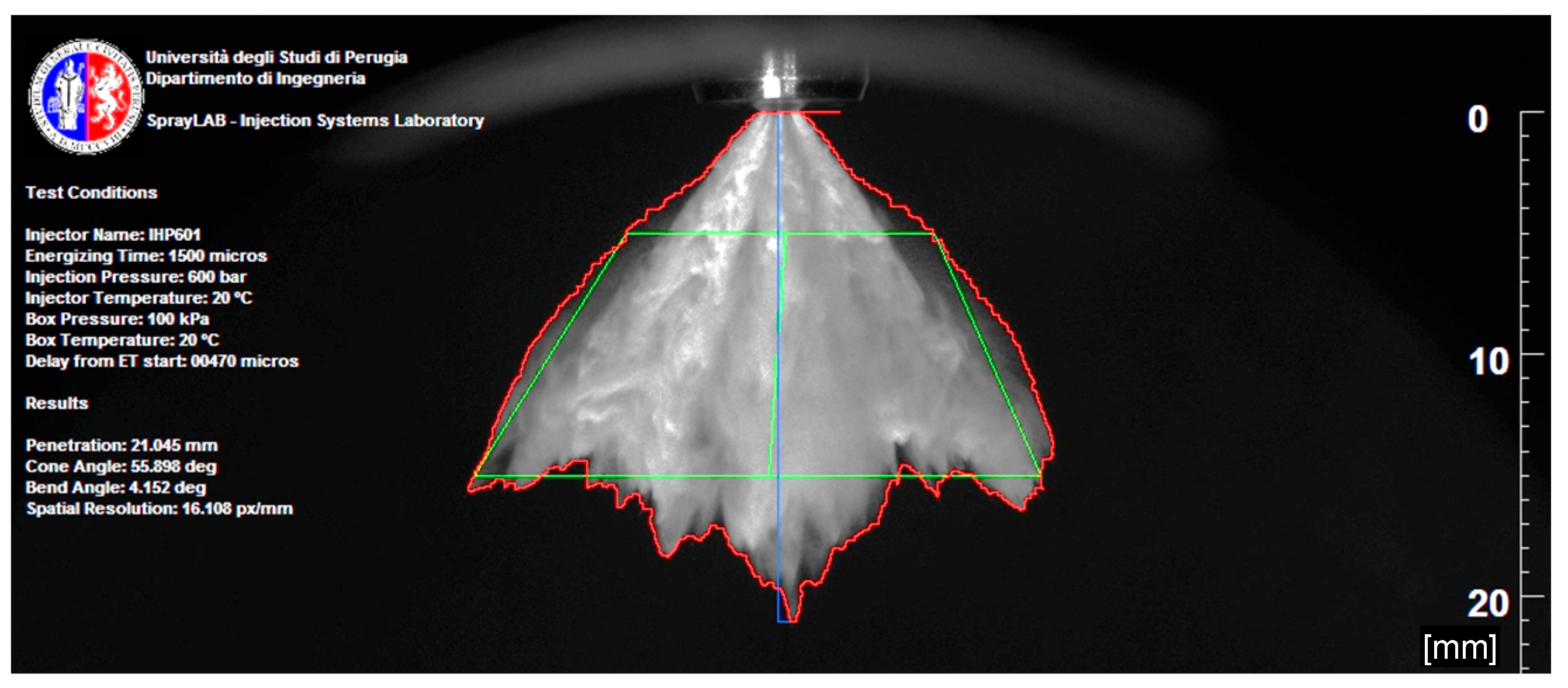
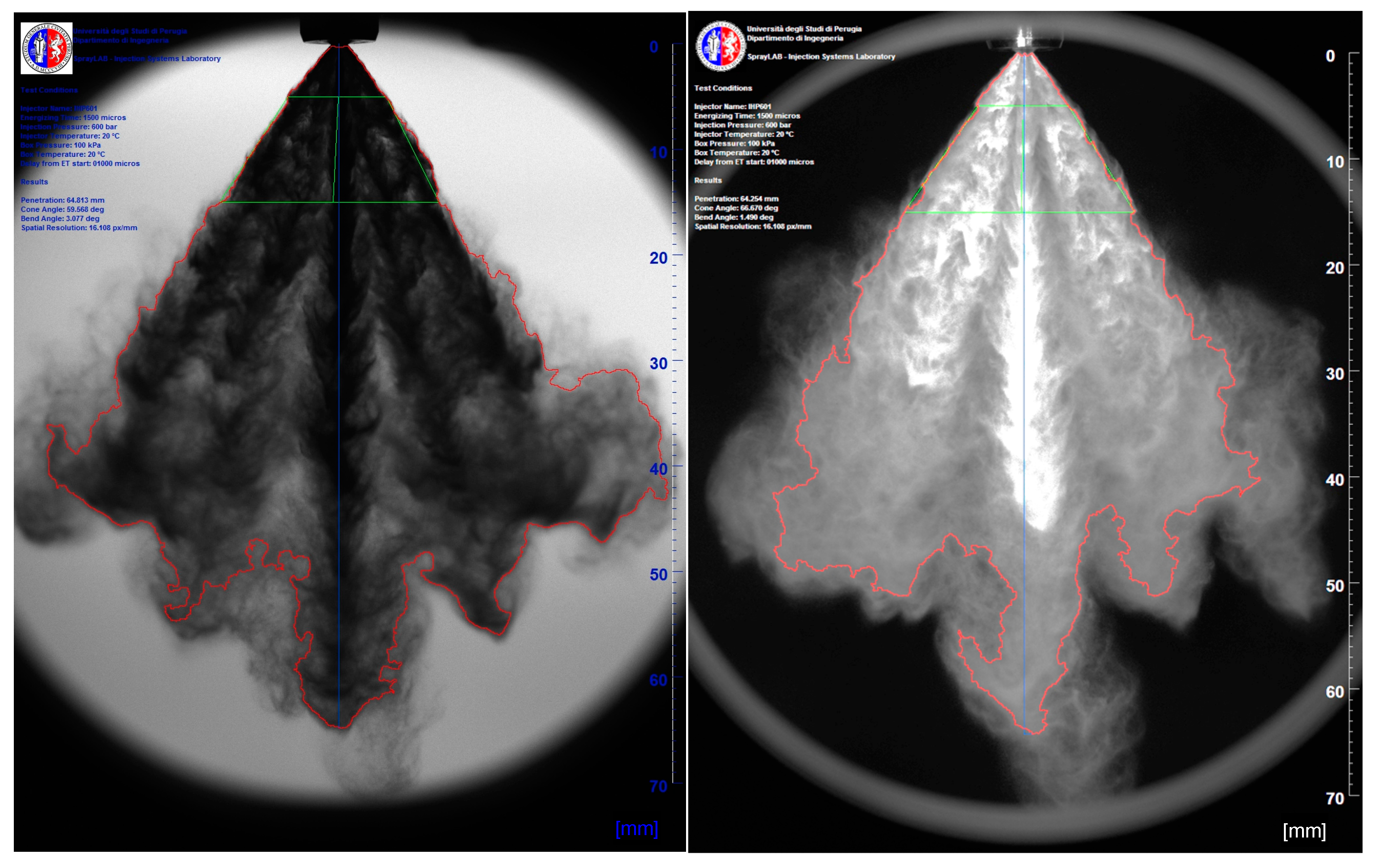
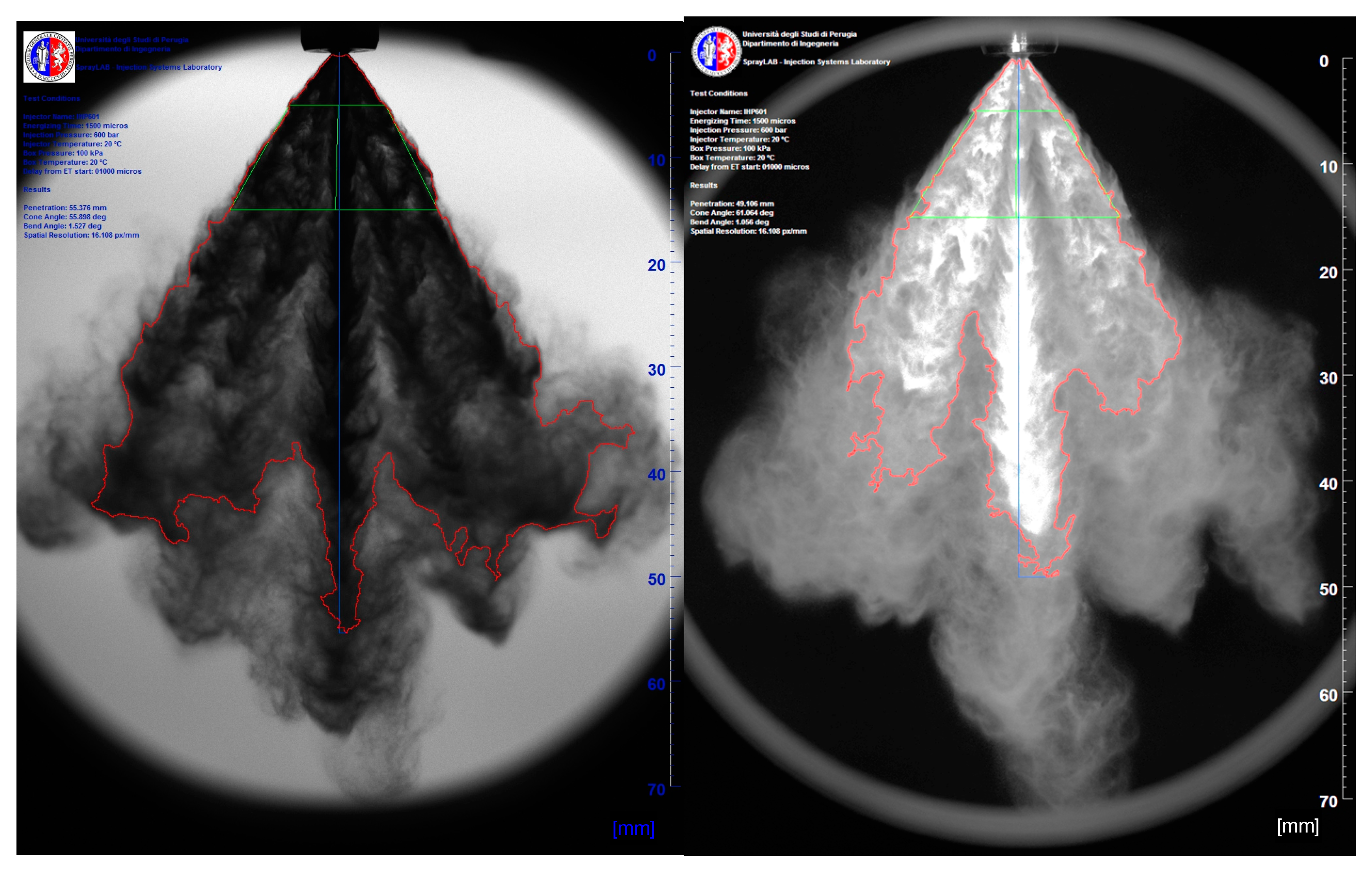
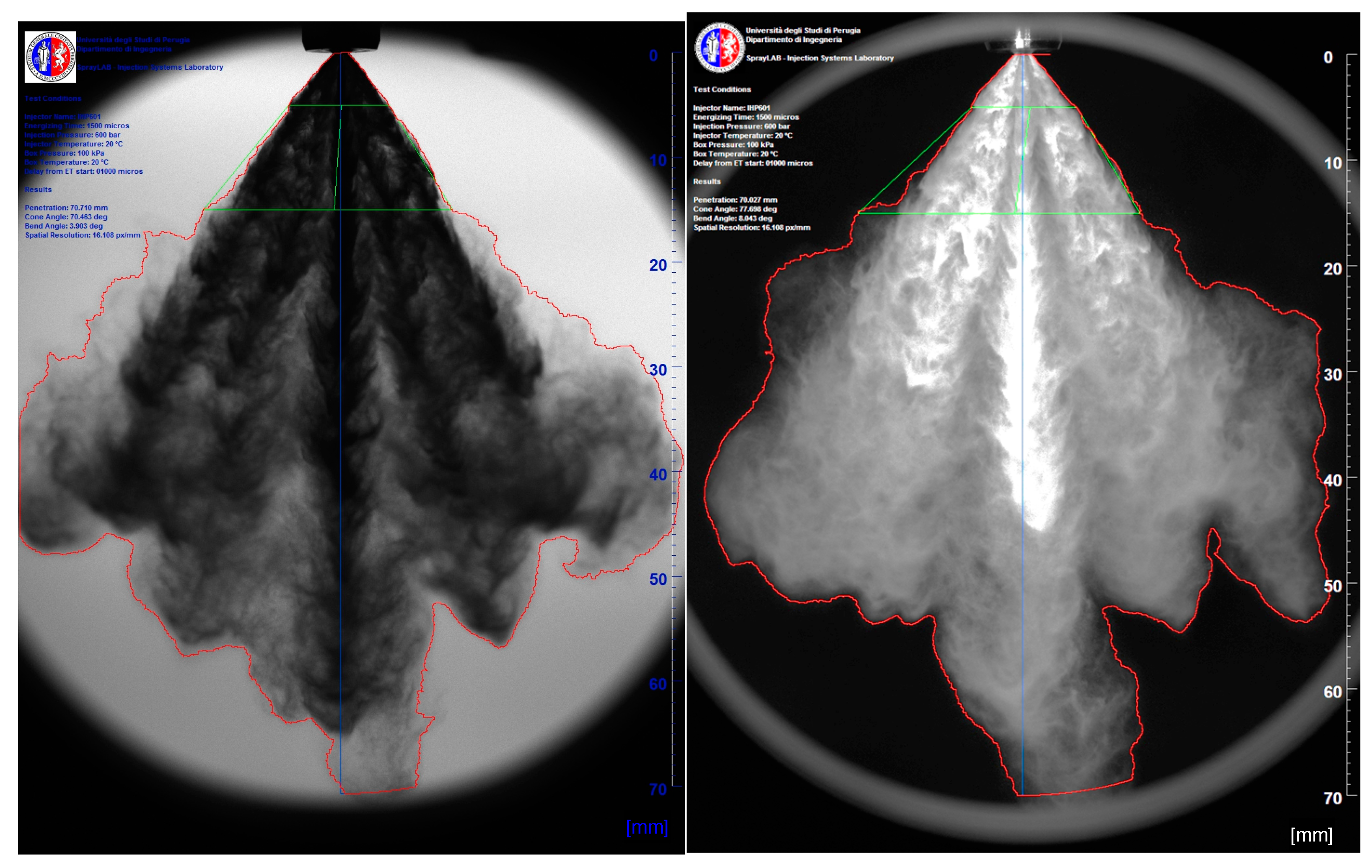
Two different sets of images are compared, the first is relevant to a timing at which the spray structure is still compact (470 μs after SOI, from Figure 8, Figure 9, Figure 10, Figure 11, Figure 12 and Figure 13); the second set is acquired at a timing in which the spray is completely developed (1000 μs after SOI, from Figure 14, Figure 15 and Figure 16). For the sake of brevity, only the results obtained at Pinj 600 bar are reported; similar results were obtained at lower injection pressure levels. In the reported images, the spray contour, the spray tip penetration, and the spray angles are evidenced by red, blue, and green lines, respectively, which were overlaid on the acquired images. The complete spray tip penetration and cone angle time-histories are reported in the plots from Figure 17, Figure 18, Figure 19 and Figure 20.
The results obtained by the three binarization methods used for the analysis can be significantly different depending on the spray structure and hence, for the same jet evolution, on the image acquisition timing.
3.1. Image Analysis Results—Partially Developed Spray
The results obtained with Pinj 600 bar for the acquisition timing of 470 µs from SOI in terms of tip penetration, cone angle, and threshold level (average values and standard deviation over the 30 images sample) are reported in Table 2.
At this timing, both in backlight and in front-light configurations, the Otsu method seems to exclude some parts of the spray in its front periphery, the tip penetration resulting moderately underestimated with respect to the other methodologies. The penetration length obtained by each method seems to be not significantly influenced by the optical setup. In terms of cone angle, while the Otsu approach results in an evident overestimation with respect to the other methodologies in backlight, while more uniform results were obtained for the front-light illumination setup. In terms of cone angle, the Otsu method results seem to be evidently affected by the optical setup. Globally, the LMC and the Yen approaches seem to be slightly more accurate than the Otsu method in detecting the spray boundary, particularly in front-light configuration, as also perceivable comparing images from Figure 8, Figure 9, Figure 10, Figure 11, Figure 12 and Figure 13.
From the same images, the LMC method identifies a spray structure boundary threshold slightly lower than the Yen method, and consequently, the spray structure area is somewhat larger. At the same time, the penetration and the cone angle results obtained by the Yen and the LMC methods are very similar, with comparable standard deviation values, as reported in Table 2. Globally, no dramatic differences were observed among the three considered methodologies in the automated detection of the spray boundary when the jet structure is relatively compact and, consequently, the spray images are characterized by net luminosity gradients.
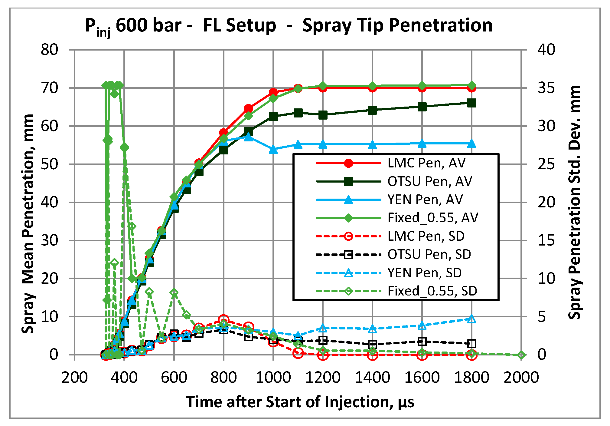
The analysis of the tip penetration curves (Figure 17 and Figure 18) confirms how the Otsu method results are similar to the results obtained by the other methods at least up to 600 µs both in backlight and front-light configuration. For later timings, the mismatch among the penetration results obtained by the considered methodologies is more significant.
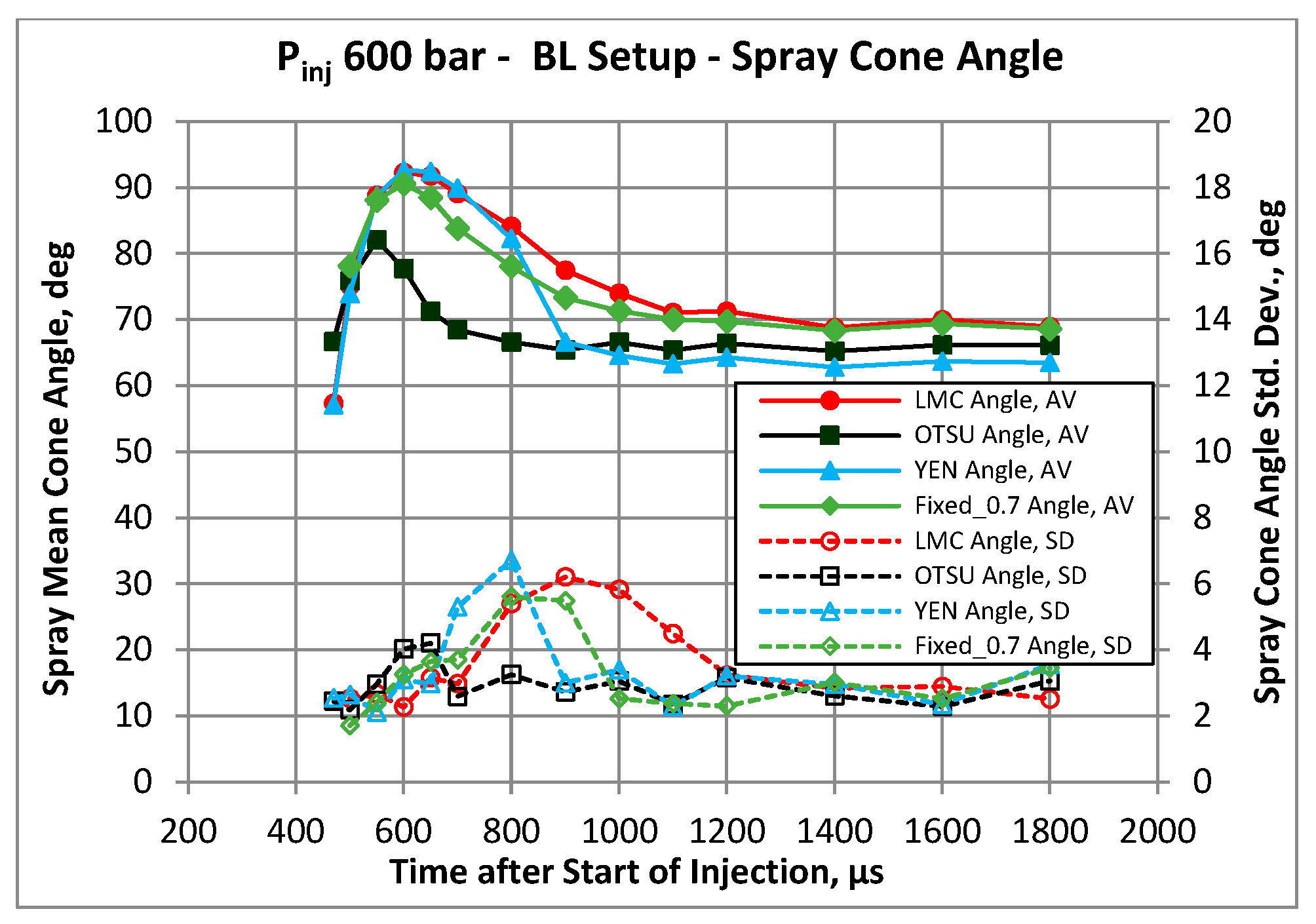
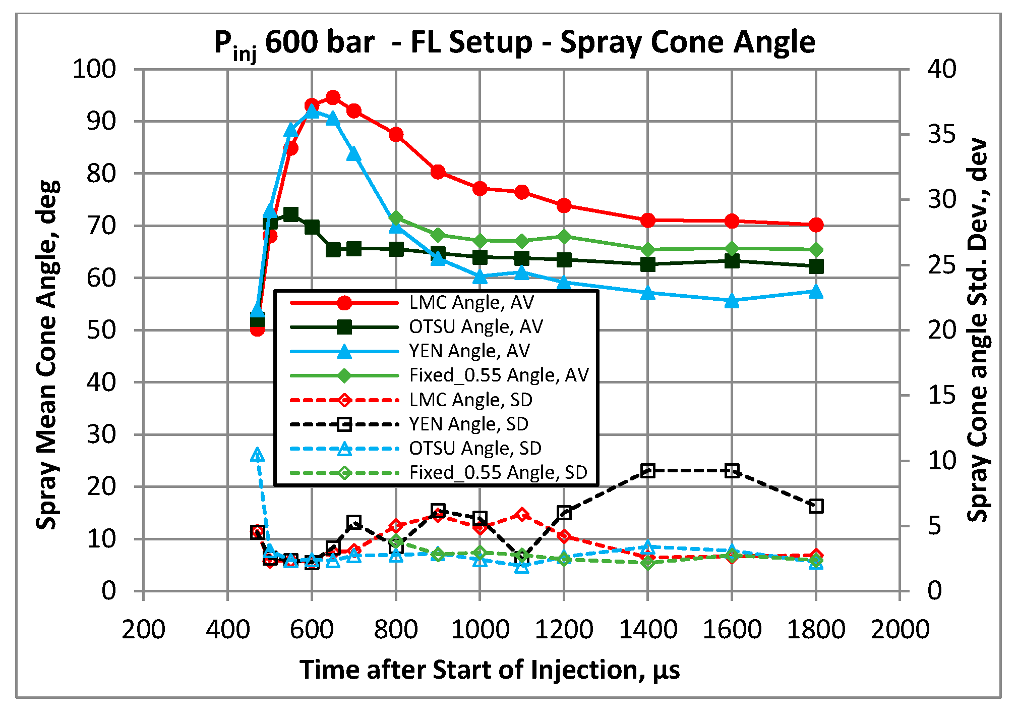
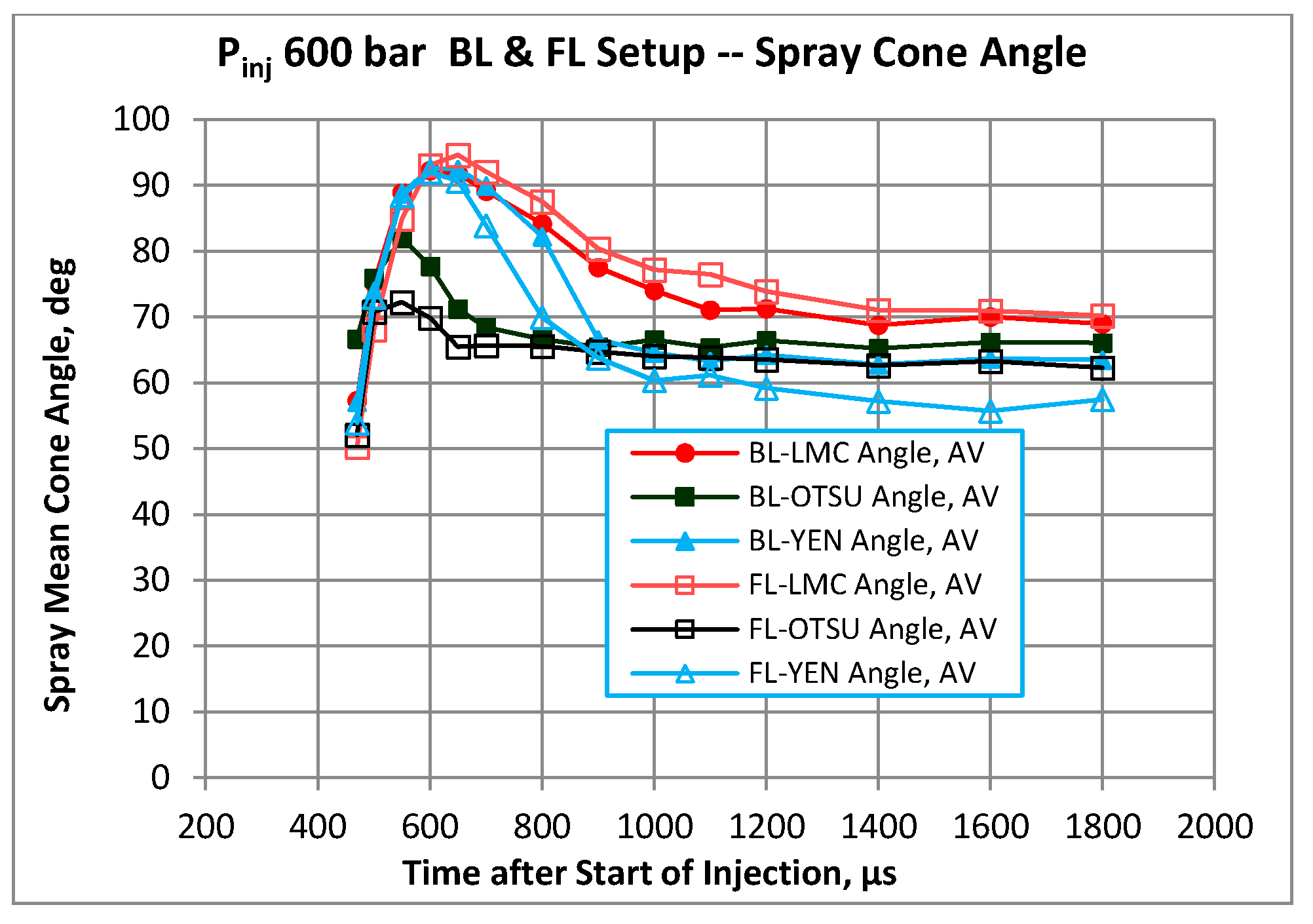
Conversely, in terms of spray cone angle, differences among the results obtained with the considered methodologies are more significant even for only partially developed sprays. In particular, the cone angles calculated by the Otsu method are remarkably different from the diffusion angles computed by the other methods. Observing Figure 19 and Figure 20, if the timing 600 μs is considered, the Otsu method cone angle results to be 77.7 deg for backlight and 69.8 deg for the front-light, with a significant dependency on the optical configuration. In the same condition and timing, the LMC and Yen methodologies yielded to very similar cone angle results: about 92.6 deg in backlight and 92.0 deg in front-light configuration, confirming a remarkable solidity regardless of the different optical setup.
Globally, considering the spray images and both the penetration and angles time histories, with only partially developed GDI sprays, the Yen method and the LMC method offered the most stable and reliable results.
3.2. Image Analysis Results—Fully Developed Spray
As discussed above, the quality of results provided by different automated image analysis algorithms can be affected by the image acquisition timing, basically as an effect of the variation of the spray apparent density during its evolution.
Considering the images reported in Figure 14, Figure 15 and Figure 16, the Last Minimum approach appears to be most efficient approach in recognizing the spray boundary in all the regions of the spray, including its side portions characterized by a very low luminosity or apparent density. Conversely, the Yen method seems to be miss significant portions of the spray structure, particularly in case of front illumination, even if characterized by remarkable high gray levels. The Otsu method shows a global behavior similar to the LMC method, but it seems to exclude from the spray structure some non-negligible spray portions both in the side periphery and on the spray tip. As for the Yen approach, the Otsu method deficiencies are particularly evident for images acquired in front-light configuration.
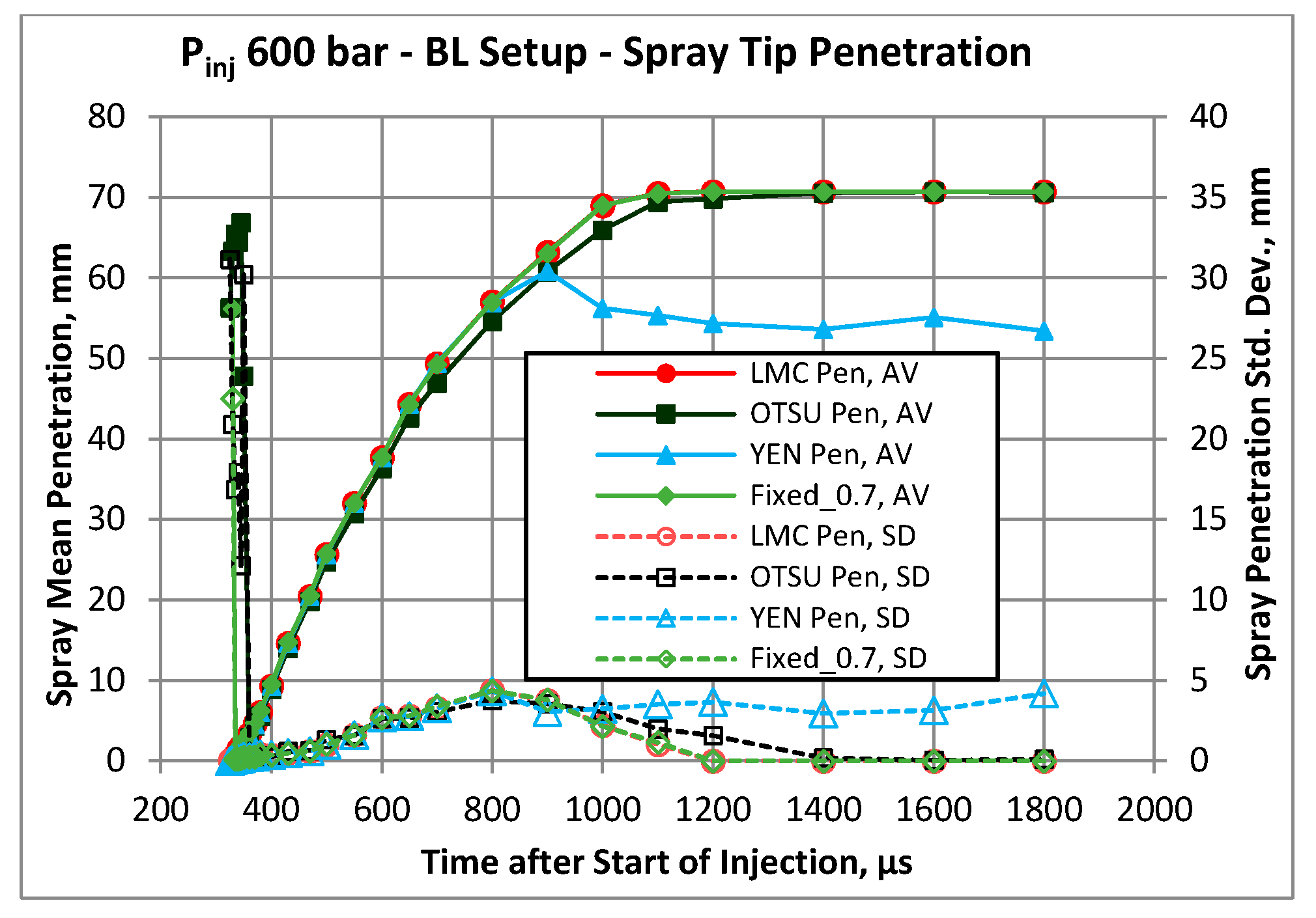
The resulting penetration time histories are reported in Figure 17 and Figure 18. Here, the three considered automated spray analysis approaches are compared also with a semi-automatic methodology where the threshold is defined as a fraction of the gray levels range defined and set by the operator. The binarization level (defined as the fraction of the available gray range from 0 to 1 and labeled in Figure 17, Figure 18, Figure 19 and Figure 20 as “Fixed_0.x” where 0.5 is the gray level) was optimized for each operating condition and applied to the analysis of the entire spray evolution. As can be seen both in terms of spray penetration (Figure 17 and Figure 18) and cone angle (Figure 19 and Figure 20), the threshold optimization can lead to somehow satisfactory results (BL setup) with the exception of the initial timings, where this method is not able to recognize the spray correctly. In different operating conditions (FL), the constant-threshold approach could not compensate the shot-to-shot light intensity dispersion, resulting in a high standard deviation. In any case, the threshold tuning must be properly carried out for every specific operating condition: in this case, different threshold levels were required for different optical setups (0.7 and 0.55, respectively for BL and FL). Different injection pressure levels (not reported here for the sake of brevity) similarly required different threshold levels from the 600 bar operating condition. For these limitations, the constant-level threshold approach will be no further considered in the present analysis.
Focusing on fully automated methodologies, as can be seen, in fully developed spray conditions, the quantitative differences caused by the compared numerical approaches are impressive: the LMC and the Otsu methods yield similar results only for the backlight configuration, while for images acquired with a front illumination, the obtained results are remarkably different. Furthermore, a remarkable dispersion for the penetration measurement carried out by the Otsu method was obtained. The spray penetration computed by the Yen method produced an evident underestimation of the spray tip penetration with both front-light and backlight configurations. Finally, when the spray tip exits the acquisition window, only the Last Minimum method in both configurations and Otsu method in front-light configuration detect the correct value of 70 mm, which represents the diameter of the acquisition window.
For the fully developed spray condition, the comparison in terms of computed spray cone angle is reported in Figure 19 and Figure 20. As can be seen, the LMC method results in larger angle values, the mismatch with the other methods being progressively reduced with the acquisition timing. The results relevant to 1.0 ms delay after SOI are reported in Table 3.
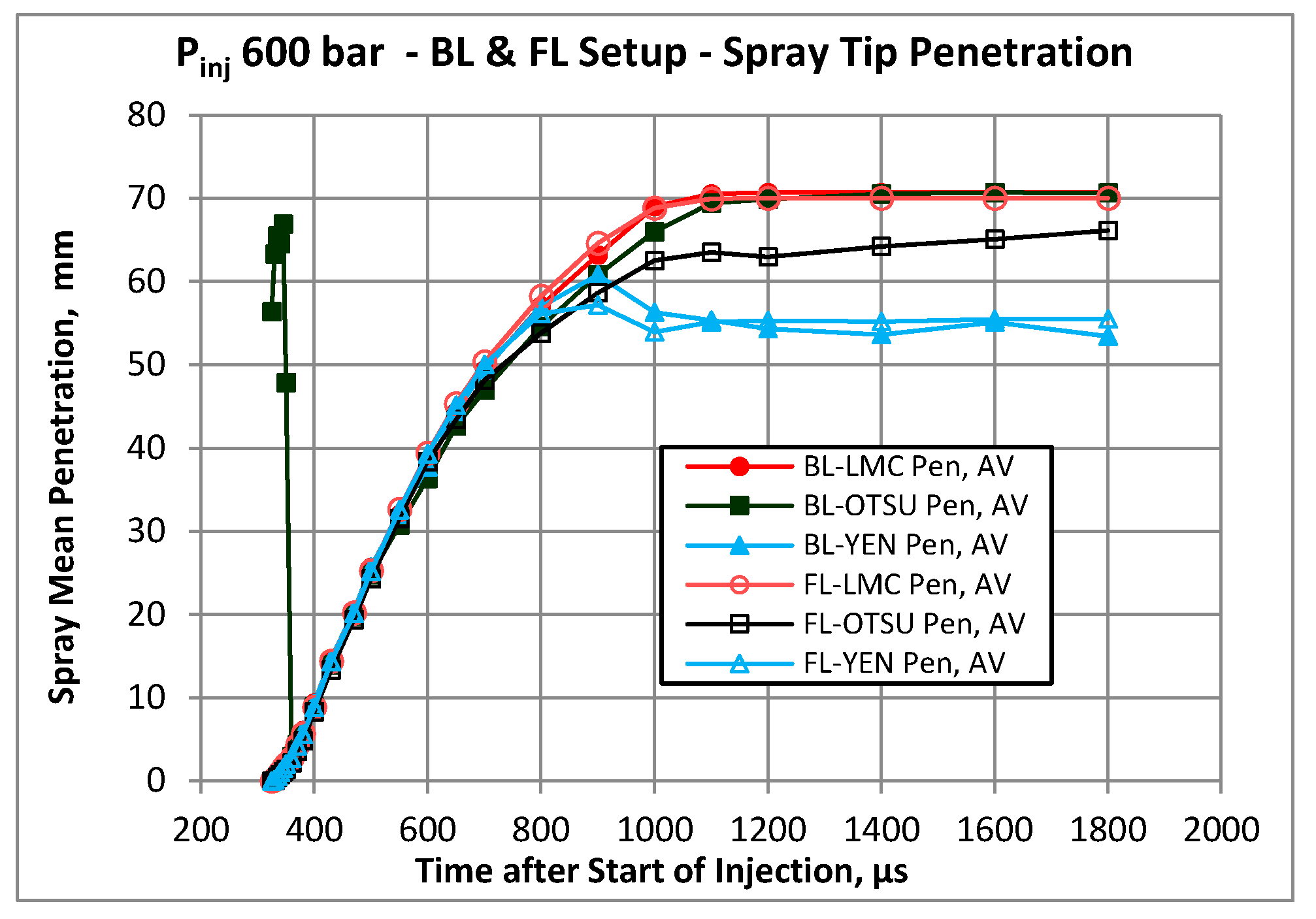
The direct comparison between penetration and cone angle results obtained by the backlight and front-light optical setups is shown in Figure 21 and Figure 22, respectively. For the penetration values, the LMC and Yen threshold detection methods produced the same trend in the two optical configurations. Conversely, the penetration trend produced by the Otsu method was evidently influenced by the used optical setup.
In terms of cone angle time histories, before the delay of 600 μs, all the compared thresholding approaches resulted in values greater in backlight than in front-light mode: as also shown in Table 2, the difference varies from about 3.1 to 14.5 deg. After 600 μs, differently from the other methods, the Last Minimum Criterion method shows cone angle values obtained for the front-light setup higher than for backlight, as shown in Table 3.
Finally, for the late acquisition timings, the LMC method allows obtaining very similar cone angle values with both front-light and backlight, proving to be more robust than the other automated thresholding methodologies.
3.3. Image Analysis Results—Injection Pressure Effect
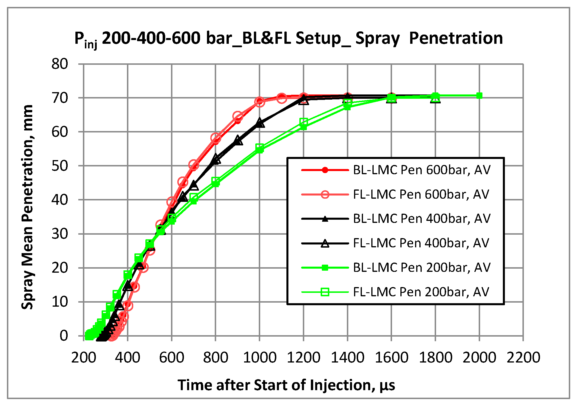
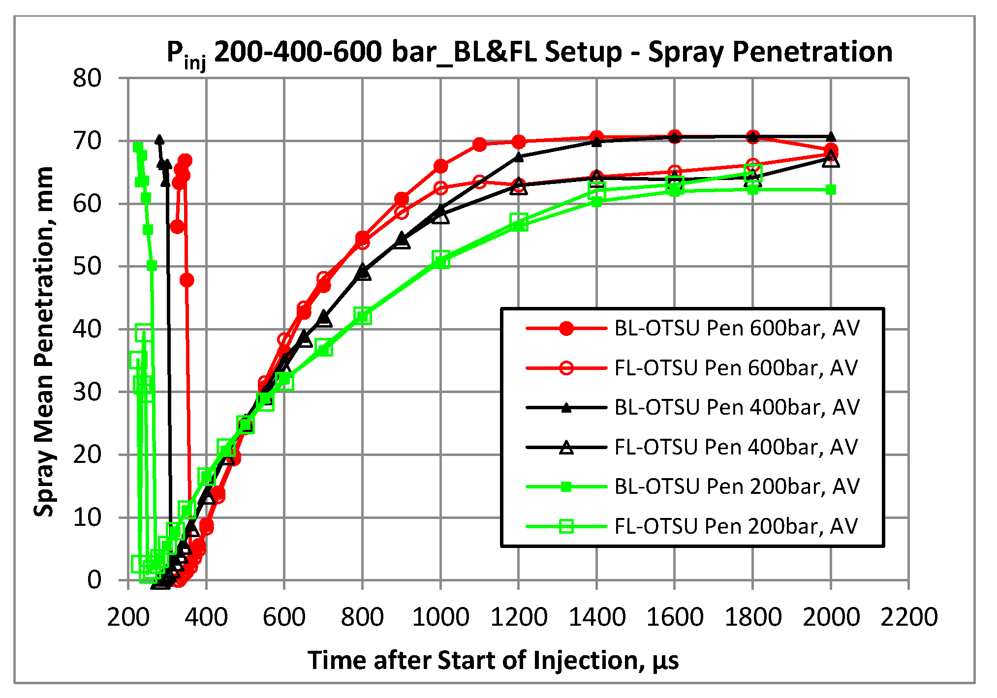
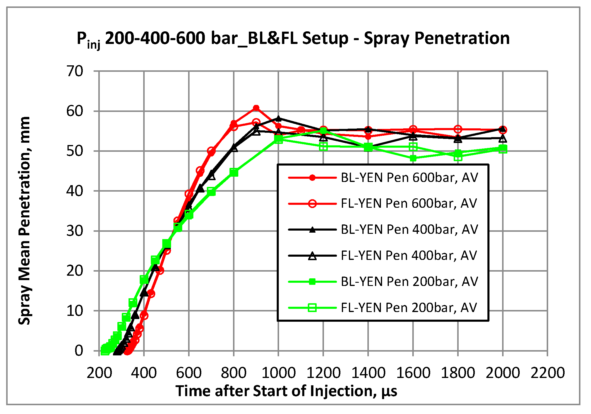
The comparisons among the image analysis results obtained with the three examined methodologies in different injection pressure levels (200, 400, and 600 bar) are presented in Figure 23, Figure 24 and Figure 25 in terms of spray tip penetration.
The penetration trends obtained with the LMC method were in agreement with the physical trend: the penetration rate grows with the injection pressure, and a steady penetration level is obtained when the spray attains the end of the visible field. The automated routine resulted to be able to detect the correct trend in all the operating conditions. Furthermore, the LMC results were not significantly affected by the used optical setup. For each injection pressure level, the two curves are very similar. The maximum difference among the front-light penetration and backlight penetration result is within 2%: 1.7 mm at 600 bar, 1.1 mm at 400 bar, and 1.5 mm at a 200 bar.
Using the Otsu method for the spray threshold computation (Figure 24), at the very beginning of the injection process, the automated routine was not able to correctly distinguish the liquid jet structure from the background, as above commented, and the penetration results are completely wrong. In the time windows elapsed from about 50 µs after the first drop appearance to the spray final development (approximately 0.8 ms after SOI), the penetration results are acceptable, with moderate discrepancies among the front-light and backlight configurations: about 2 mm at 600 bar, 1.6 mm at 400 bar, and 0.5 mm at 200 bar. In the spray final development phase, the Otsu method resulted in significantly different penetration results for front-light and backlight optical layouts: about 6 mm at 600 bar, 7 mm at 400 bar, and 8 mm at 200 bar.
Figure 25 presents the penetration results obtained by the Yen method. This thresholding methodology proved to be efficient with both the backlight and front-light configurations in the analysis of a compact spray structure: before 700 µs delay, the maximum difference among FL and BL configuration is 1.6 mm at 600 bar, 0.9 mm at 400 bar, and 0.5 mm at 200 bar. The observed spray penetration trend in these conditions is very similar to the trend obtained by the LMC method. When the spray enters its final development phase and its apparent density starts to decrease significantly (around 0.7 ms after SOI), the Yen approach proved to be very sensitive to the optical setup: the maximum difference among FL and BL is 3.6 mm at 600 bar, 5 mm at 400 bar, and 4 mm at 200 bar. It is worth noting that the Yen method failed to correctly detect the spray exit from the visible zone that should result in a saturation of the penetration curves.
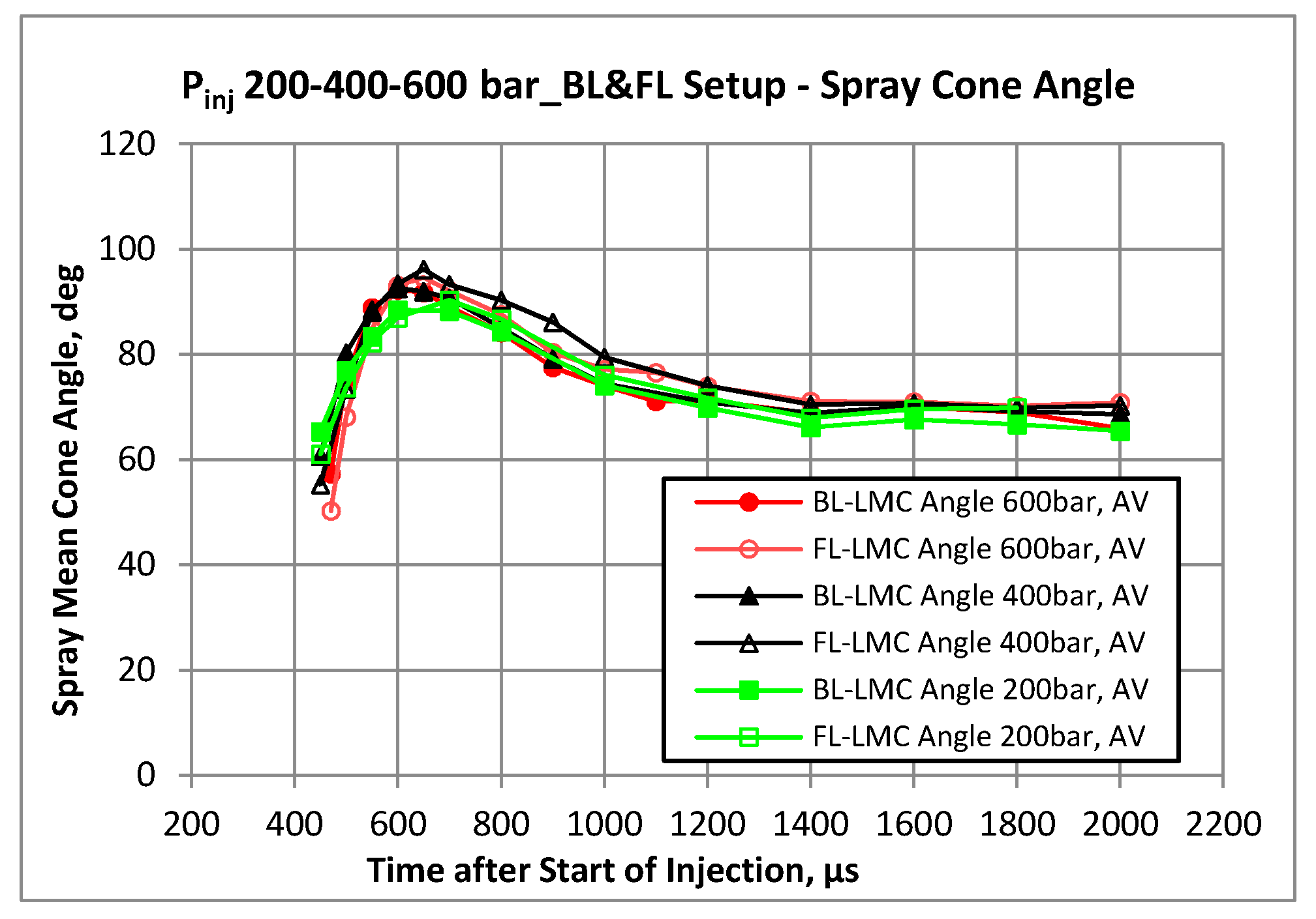
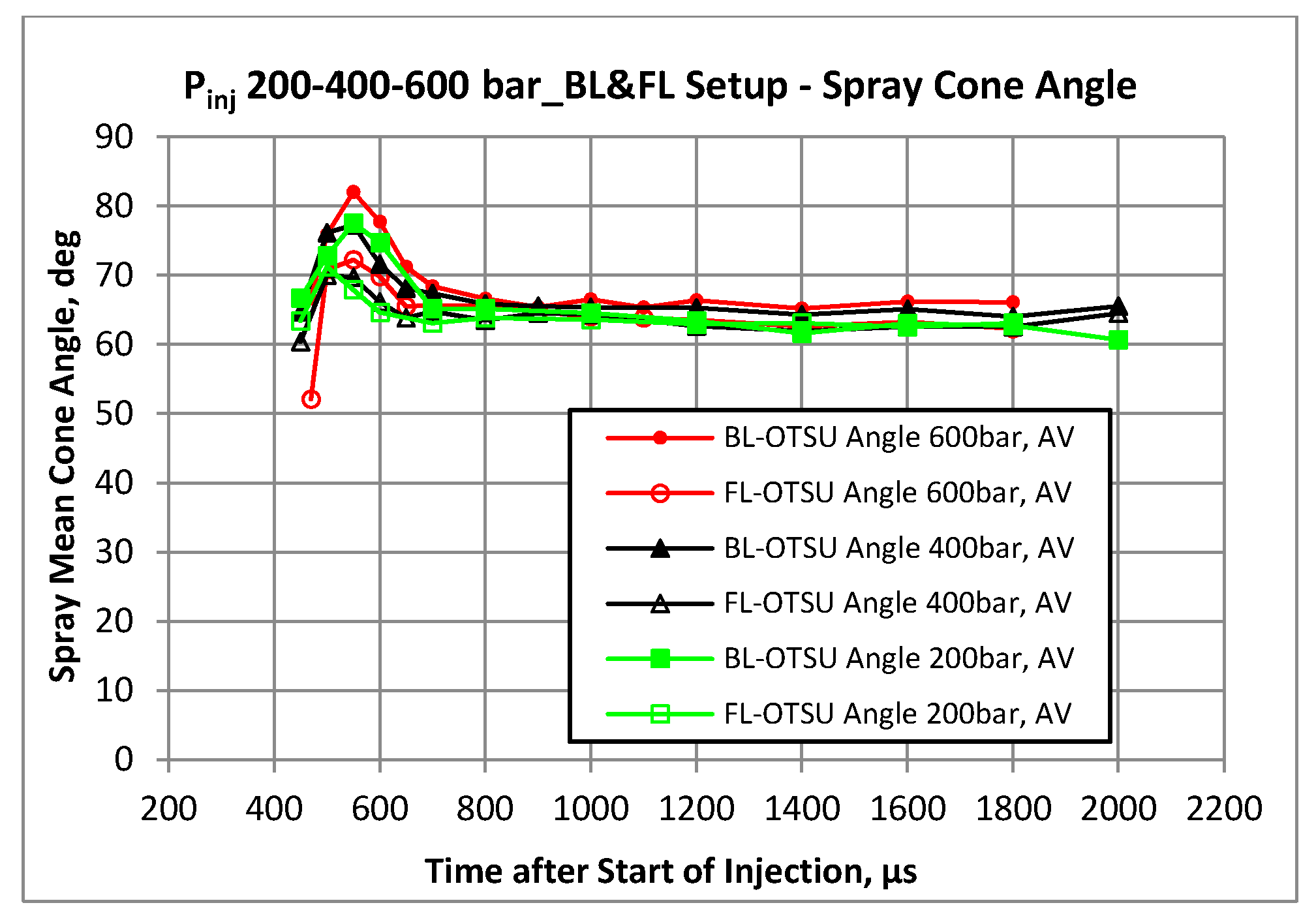
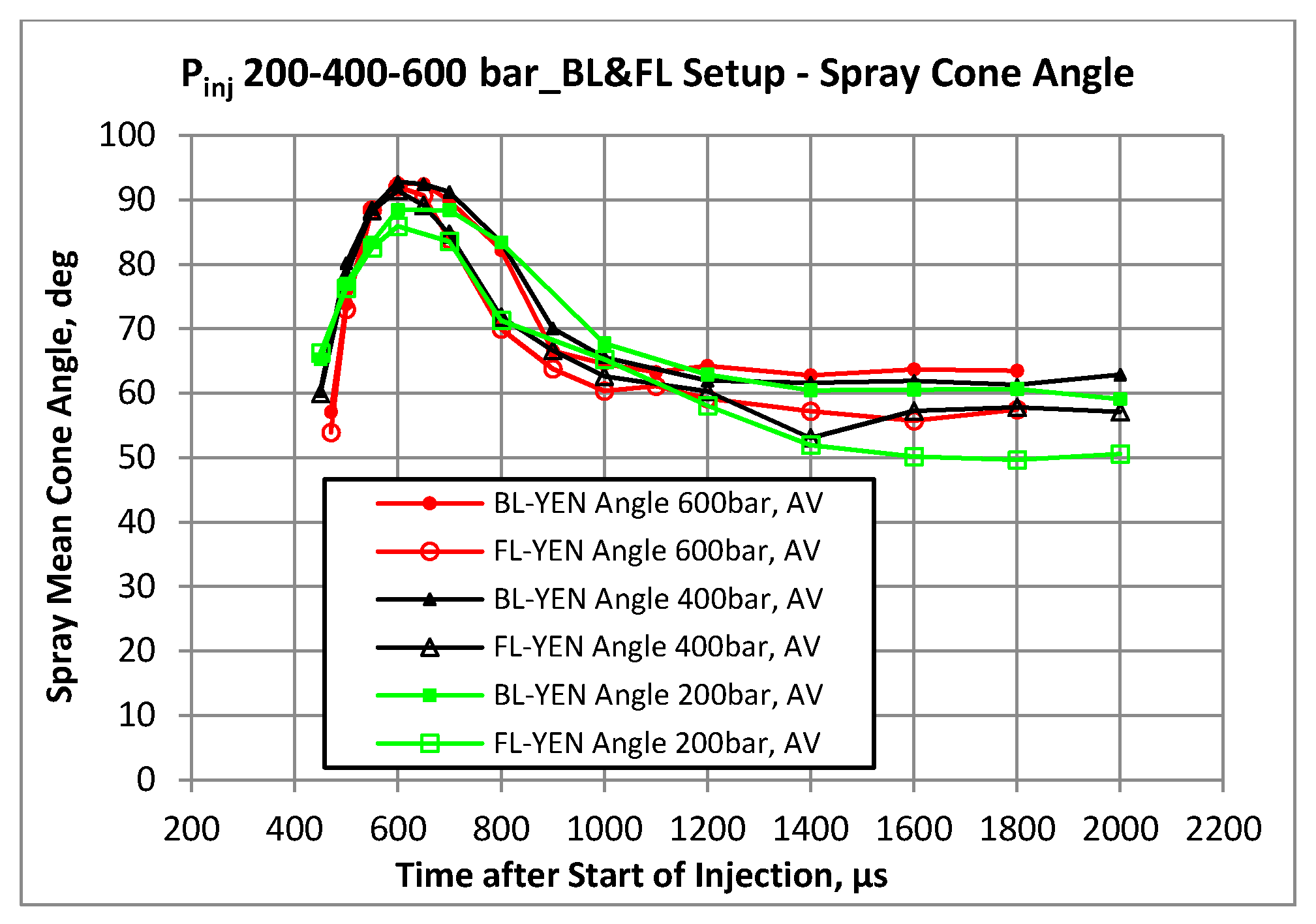
The comparisons among the spray angle results obtained with the examined methodologies are shown in Figure 26, Figure 27 and Figure 28. The general trends commented for the operating condition Pinj 600 bar are confirmed: the most significant differences are observed for the first part of the spray evolution, where the LMC method seems to be better able to detect the spray structure side boundary and consequently yields to larger cone angle values. Conversely, in the final part of the spray evolution, when the cone angle trend flattens to an almost constant value, smaller differences among the three methodologies are obtained. In the very final part of the spray evolution following the injection process end, neither the Yen method nor the Otsu method seem to be completely adequate for the automated spray boundary detection, resulting in erroneous spray cone angle values. In particular, the Yen method was observed to produce spray angle results susceptible to the optical setup used for the image acquisition, with significant differences among backlight and front-light results.
4. Conclusions
In the present paper, an innovative procedure for the automated analysis of GDI spray images is presented and discussed. The crucial step in automated spray analysis procedure is binarization, by which the spray structure is distinguished from the background, enabling the next phases in which the geometrical parameters describing the spray evolution are computed.
The proposed binarization approach—named Last Minimum Criterion, LMC—is derived from the well-known Triangle method; according the LMC approach, in the analysis of the gray-level frequency probability histogram, only the second to last local maximum is considered to locate the gray-level threshold used to identify the spray-relevant gray levels. This proposed algorithm is comparatively validated along with the well-diffused Otsu and Yen methods. To this end, these three criteria were used for the analysis of high-pressure GDI sprays, images being acquired with three injection pressure levels (up to 600 bar) and two different optical setups (backlight and front illumination), thus using a challenging dataset. In computing the main geometrical spray parameters (tip penetration and angle), the prescriptions suggested by the SAEJ 2715 rule were followed. The following main results were obtained:
- -
- LMC allows the adequate recognition of the spray boundary throughout the entire spray evolution, from the initial phase in which the spray appears as very compact to the final development phase, in which the spray structure is very fragmented and dispersed. Satisfactory results were obtained both with the backlight and front light optical setups. Conversely, the application of both the Otsu and Yen methods resulted in a generally poor spray pattern recognition, with significant parts of the spray excluded from the analysis.
- -
- In terms of spray tip penetration, the Otsu method offered erratic results in the very first part of the spray evolution, while a better accuracy was obtained in the late acquisition timings (completely developed spray) with a backlight optical configuration. For the analysis of front-lighted spray images, the Otsu method under-estimated tip penetration. The spray cone angle was generally underestimated by the Otsu binarization criterion, particularly in the first part of the spray evolution; the optical setup marginally affected the final spray evolution angle results.
- -
- The Yen binarization algorithm resulted in satisfactory spray penetration time-profile curves in the initial part of the spray evolution but evidently underestimated penetration levels were observed for fully developed GDI spray conditions. Similarly, cone angle results were satisfactory only for the initial acquisition timing, while this algorithm proved to be less efficient when the spray compactness was reduced. This method efficacy was appreciably similar with both backlight and front light optical illumination strategies.
- -
- The results obtained varying the injection pressure level from 200 to 600 bar confirmed the above reported trends.
Globally, the proposed LMC offered encouraging results in enabling the development of a completely automated image analysis procedure for GDI injection systems testing, providing reliable results in a wide range of operating conditions and with different optical setups.
The proposed algorithm efficacy will be investigated also for the analysis of spray images of other challenging datasets, particularly low-pressure sprays of gasoline and diesel exhaust fluid.
Author Contributions
Conceptualization, L.P. and F.R.; methodology, L.P. and F.R.; software, F.R.; validation, L.P. and F.R.; investigation, L.P. and F.R.; resources, L.P.; data curation, L.P. and F.R.; writing—original draft preparation, L.P. and F.R.; writing—review and editing, L.P.; visualization, L.P. and F.R.; supervision, L.P.; project administration, L.P.; funding acquisition, L.P. All authors have read and agreed to the published version of the manuscript.
Funding
This research received no external funding.
Institutional Review Board Statement
Not applicable.
Informed Consent Statement
Not applicable.
Data Availability Statement
Data available on request due to restrictions eg privacy or ethical.
Acknowledgments
The authors wish to thank Magneti Marelli for having provided the GDI injector used for the tests.
Conflicts of Interest
The authors declare no conflict of interest.
References
- Canny, J. A Computational Approach to Edge Detection. IEEE Trans. Pattern Anal. Mach. Intell. 1986, 8, 679–698. [Google Scholar] [CrossRef] [PubMed]
- Klein-Douwel, R.J.H.; Frijters, P.J.M.; Somers, L.M.T.; de Boer, W.A.; Baert, R.S.G. Macroscopic diesel fuel spray shadowgraphy using high speed digital imaging in a high pressure cell. Fuel 2007, 86, 1994–2007. [Google Scholar] [CrossRef]
- Sezgin, M.; Sankur, B. Survey over image thresholding techniques and quantitative performance evaluation. J. Electron. Imaging 2004, 13, 146–168. [Google Scholar] [CrossRef]
- Otsu, N. A threshold selection method from gray-level histograms. IEEE Trans. Syst. Man Cybern. 1979, 9, 62–66. [Google Scholar] [CrossRef] [Green Version]
- Yen, J.-C.; Chang, F.-J.; Chang, S. A new criterion for automatic multilevel thresholding. IEEE Trans. Image Process. 1995, 4, 370–378. [Google Scholar] [CrossRef] [PubMed]
- Naber, J.D.; Siebers, D.L. Effects of Gas Density and Vaporization on Penetration and Dispersion of Diesel Sprays; SAE Paper 960034; SAE International: Warrendale, PA, USA, 1996. [Google Scholar]
- Zack, G.W.; Rogers, W.E.; Latt, S.A. Automatic measurement of sister chromatid exchange frequency. J. Histochem. Cytochem. 1977, 25, 741–753. [Google Scholar] [CrossRef] [PubMed]
- Postrioti, L.; Bosi, M.; Mariani, A.; Ungaro, C. Momentum Flux Spatial Distribution and PDA Analysis of a GDI Spray; SAE Technical Paper 2012-01-0459; SAE International: Warrendale, PA, USA, 2012. [Google Scholar]
- Postrioti, L.; Malaguti, S.; Bosi, M.; Buitoni, G.; Piccinini, S.; Bagli, S. Experimental and numerical characterization of a direct solenoid actuation injector for Diesel engine applications. Fuel 2014, 118, 316–328. [Google Scholar] [CrossRef]
- Postrioti, L.; Bosi, M.; Cavicchi, A.; Abuzahra, F.; Di Gioia, R.; Bonandrini, G. Momentum Flux Measurement on Single-Hole GDI Injector under Flash-Boiling Condition; SAE Technical Paper 2015-24-2480; SAE International: Warrendale, PA, USA, 2015. [Google Scholar] [CrossRef]
- Hung, D.L.; Harrington, D.L.; Gandhi, A.H.; Markle, L.E.; Parrish, S.E.; Shakal, J.S.; Sayar, H.; Cummings, S.D.; Kramer, J.L. Gasoline Fuel Injector Spray Measurement and Characterization—A New SAE J2715 Recommended Practice. SAE Int. J. Fuels Lubr. 2008, 1, 534–548. [Google Scholar] [CrossRef]
Figure 1.
Example of spray image frequency histogram—backlight.

Figure 2.
Triangle Method: threshold identification [7].
Figure 2.
Triangle Method: threshold identification [7].

Figure 3.
Image histogram of a late-timing spray image.

Figure 4.
The Last Minimum Criterion (LMC).

Figure 5.
Backlight configuration.

Figure 6.
Front-light configuration, external view.

Figure 7.
Synchronization system configuration.

Figure 8.
Pinj 600 bar, 470 μs after SOI—BL, Otsu method.

Figure 9.
Pinj 600 bar, 470 μs after SOI—BL, Yen method.

Figure 10.
Pinj 600 bar, 470 μs after SOI—BL, LMC method.

Figure 11.
Pinj 600 bar, 470 μs after SOI—FL, Otsu method.

Figure 12.
Pinj 600 bar, 470 μs after SOI—FL, Yen method.

Figure 13.
Pinj 600 bar, 470 μs after SOI—FL, LMC method.

Figure 14.
Pinj 600 bar, 1 ms after SOI-Otsu.

Figure 15.
Pinj 600 bar, 1 ms after SOI-Yen.

Figure 16.
Pinj 600 bar, 1 ms after SOI-LMC.

Figure 17.
Spray tip penetration—backlight setup.

Figure 18.
Spray tip penetration—front-light setup.

Figure 19.
Spray cone angle—backlight setup.

Figure 20.
Spray cone angle—front-light setup.

Figure 21.
Pinj 600 bar—penetration—backlight and front-light configurations.

Figure 22.
Pinj 600 bar—cone angle—backlight and front-light configurations.

Figure 23.
Penetration BL-FL—pressure comparison, LMC method.

Figure 24.
Penetration BL-FL—pressure comparison, Otsu method.

Figure 25.
Penetration BL-FL—pressure comparison, Yen method.

Figure 26.
Cone angle BL-FL—pressure comparison, Last Minimum method.

Figure 27.
Penetration BL-FL—pressure comparison, Otsu method.

Figure 28.
Penetration BL-FL—pressure comparison, Yen method.


Table 1.
Injector current parameters.
| Parameters | Values |
|---|---|
| Peak Current | 12 A |
| Duration of Peak Current | 700 µs |
| Hold Current | 2.6 A |
Table 2.
Pinj 600 bar, spray @ 470 µs from SOI. Penetration, cone angle and threshold level by LMC, Otsu and Yen methods.
Table 2.
Pinj 600 bar, spray @ 470 µs from SOI. Penetration, cone angle and threshold level by LMC, Otsu and Yen methods.
| Backlight | Front-Light | |||||
|---|---|---|---|---|---|---|
| LMC | Otsu | Yen | LMC | Otsu | Yen | |
| Penetration [mm] | 20.45 | 19.83 | 20.47 | 20.20 | 19.37 | 20.13 |
| Penetration, std. dev. [mm] | 0.59 | 0.66 | 0.60 | 0.59 | 0.65 | 0.60 |
| Cone Angle [deg] | 57.32 | 66.68 | 57.09 | 50.24 | 52.10 | 53.90 |
| Cone Angle, std.dev. [deg] | 2.53 | 2.45 | 2.54 | 4.63 | 10.51 | 4.53 |
| Threshold [n.d.] | 1244 | 777 | 1250 | 90 | 843 | 119 |
| Threshold, std.dev. [n.d.] | 14 | 8 | 14 | 2 | 16 | 5 |
Table 3.
Pinj 600 bar, spray @ 1 ms from SOI. Penetration, cone angle, and threshold level obtained by LM, Otsu, and Yen methods.
Table 3.
Pinj 600 bar, spray @ 1 ms from SOI. Penetration, cone angle, and threshold level obtained by LM, Otsu, and Yen methods.
| BL | FL | |||||
|---|---|---|---|---|---|---|
| LMC | Otsu | Yen | LMC | Otsu | Yen | |
| Pen, AV | 69.01 | 65.97 | 56.26 | 68.84 | 62.51 | 53.94 |
| Pen, SD | 2.22 | 3.07 | 3.26 | 1.76 | 2.01 | 2.99 |
| Cone, AV | 74.02 | 66.53 | 64.57 | 77.17 | 64.01 | 60.36 |
| Cone, SD | 4.49 | 3.05 | 3.40 | 4.86 | 2.43 | 5.60 |
| Thresh, AV | 1190 | 833 | 652 | 102 | 939 | 1403 |
| Thresh, SD | 15 | 10 | 52 | 7 | 27 | 184 |
Publisher’s Note: MDPI stays neutral with regard to jurisdictional claims in published maps and institutional affiliations. |
© 2021 by the authors. Licensee MDPI, Basel, Switzerland. This article is an open access article distributed under the terms and conditions of the Creative Commons Attribution (CC BY) license (http://creativecommons.org/licenses/by/4.0/).
Share and Cite
MDPI and ACS Style
Rosignoli, F.; Postrioti, L. Experimental Validation of an Innovative Approach for GDI Spray Pattern Recognition. Fuels 2021, 2, 16-36. https://0-doi-org.brum.beds.ac.uk/10.3390/fuels2010002
AMA Style
Rosignoli F, Postrioti L. Experimental Validation of an Innovative Approach for GDI Spray Pattern Recognition. Fuels. 2021; 2(1):16-36. https://0-doi-org.brum.beds.ac.uk/10.3390/fuels2010002
Chicago/Turabian StyleRosignoli, Federico, and Lucio Postrioti. 2021. "Experimental Validation of an Innovative Approach for GDI Spray Pattern Recognition" Fuels 2, no. 1: 16-36. https://0-doi-org.brum.beds.ac.uk/10.3390/fuels2010002