New Hybrid Approach for Developing Automated Machine Learning Workflows: A Real Case Application in Evaluation of Marcellus Shale Gas Production

Abstract

The success of machine learning (ML) techniques implemented in different industries heavily rely on operator expertise and domain knowledge, which is used in manually choosing an algorithm and setting up the specific algorithm parameters for a problem. Due to the manual nature of model selection and parameter tuning, it is impossible to quantify or evaluate the quality of this manual process, which in turn limits the ability to perform comparison studies between different algorithms. In this study, we propose a new hybrid approach for developing machine learning workflows to help automated algorithm selection and hyperparameter optimization. The proposed approach provides a robust, reproducible, and unbiased workflow that can be quantified and validated using different scoring metrics. We have used the most common workflows implemented in the application of artificial intelligence (AI) and ML in engineering problems including grid/random search, Bayesian search and optimization, genetic programming, and compared that with our new hybrid approach that includes the integration of Tree-based Pipeline Optimization Tool (TPOT) and Bayesian optimization. The performance of each workflow is quantified using different scoring metrics such as Pearson correlation (i.e., R² correlation) and Mean Square Error (i.e., MSE). For this purpose, actual field data obtained from 1567 gas wells in Marcellus Shale, with 121 features from reservoir, drilling, completion, stimulation, and operation is tested using different proposed workflows. A proposed new hybrid workflow is then used to evaluate the type well used for evaluation of Marcellus shale gas production. In conclusion, our automated hybrid approach showed significant improvement in comparison to other proposed workflows using both scoring matrices. The new hybrid approach provides a practical tool that supports the automated model and hyperparameter selection, which is tested using real field data that can be implemented in solving different engineering problems using artificial intelligence and machine learning. The new hybrid model is tested in a real field and compared with conventional type wells developed by field engineers. It is found that the type well of the field is very close to P50 predictions of the field, which shows great success in the completion design of the field performed by field engineers. It also shows that the field average production could have been improved by 8% if shorter cluster spacing and higher proppant loading per cluster were used during the frac jobs.

1. Introduction

The application of Artificial intelligence (AI) in general and machine learning (ML) specifically has gained lots of popularity in the past few years throughout various industries including the oil and gas industry. This rise in popularity is especially due to the application of new technologies such as sensors and high-performance computing services that enable big-data acquisition and storage [1,2].

For a specific engineering problem, in which adhering to the observation data is not sufficient and physics of the problem must be honored as well, searching for the best pre-processing techniques and machine learning model (or the best combination of different machine learning models) is a comprehensive task, especially if automated machine learning is not implemented. It is a fact that there are multiple great pre-processing techniques and ML models available with different levels of complexity that can serve to solve a specific problem. Therefore, the selection of the best one within that pool of models (for a dataset) is certainly not straightforward. In addition, within a selected ML model, optimization of its hyperparameters is involved with a certain complexity. In [3], it was shown that the configuration of hyperparameters is even more important than the model selection and proved that an efficient model can be obtained for a specific classification problem solely based on hyperparameter choice. Therefore, there is a critical need to restructure manual and traditional machine learning workflows such that human bias in model selection and hyperparameter optimization will be eliminated by using some sort of automated and integrated approach that can be evaluated and quantified using scoring metrics to ensure robustness and reproducibility of the results.

Using recent development in automated machine learning, this paper introduces a new hybrid approach to address common problems associated with manual machine learning selection and hyperparameter optimization using large-scale real field data. The hybrid approach combines the strength of Automatic Machine Learning (AML) using Tree-based Optimization Tool (TPOT), Bayesian hyperparameter search, and Bayesian optimization. This hybrid approach quantifies its efficacy in use for data analytics of high-dimensional data in oil and gas, as it excels other proposed approaches to be studied in this paper.

2. Methodology

In this study, we focus on the application of different ML workflows in engineering-based problems, in which the physics-based data-driven approach will be used to optimize an engineering workflow. The difference between engineering versus non-engineering applications of the ML approach is that in addition to adhering to the observation data, the data-driven model also needs to honor the physics of the problem. To make sure this criterion has been satisfied, the external knowledge of the problem will be imposed into the workflow during data pre-processing by introducing the physics of each feature by assigning the intrinsic statistical characteristics of each feature such as feature probability density function, covariance functions, and cross-validation of anomalies and outliers with actual physics of the feature. For this purpose, the same data pre-processing approach has been used for all the workflows. To ensure the robustness of our approach, the automated pre-processing offered by the Tree-based Pipeline Optimization Tool (TPOT) is also performed [4] and the result is compared with the proposed physics-based data pre-processing approach.

The methodology of this paper follows four major tasks, including: (1) data pre-processing, (2) algorithms configuration, (3) design of workflows, and (4) scoring metrics for the designed workflows. Each task is then divided into necessary sub-tasks, as shown by the ordered bullet points.

2.1. Data Pre-Processing

We have used our domain expertise in the oil and gas industry to preserve the statistical properties of features and conduct necessary data transformation, before applying any ML workflow. The original dataset used for this study involves data collected from 1567 unconventional gas wells and 121 recorded features. These features are categorized into seven groups: Well API, Trajectory, Perforation, Injection schedule, Logging and Geomechanics, Operations, Production, and Others. A summary of the features in the dataset is presented in

Table 1. Summary of the features in the original dataset.

Group	Examples of Features	Number of Features
G0—Well API	API, Well number, Well Index	7
G1—Trajectory	MD, TVD, Easting, Northing	10
G2—Perforation	Cluster Spacing, Perforation Stage	9
G3—Injection schedule	Proppant loading, Water loading, Proppant meshes, Fracture Gradient	17
G4—Logging and Geomechanics	Impedance, Young Modulus, Clay Volume, Gas Content	27
G5—Operations	Casing Pressure, Tubing Pressure	24
G6—Production	Cumulative/normalized production data (90/180/360/540 days)	20
G7—Others	BTU, frac hit	7

. All relevant pre-processing techniques are briefly described below.

(a)

Primary scanning

The first subtask in data pre-processing is the primary scanning process, which removes all features that have an amount of missing data exceeding 20% of the total amount of wells, i.e., all wells that miss production and/or trajectory data are removed from the dataset.

(b)

Detachment of characteristic features

Next, a feature that considers characteristic inputs such as well number or pad/field number is identified. These features are not necessary for later tasks such as handling missing values, removal of outliers or applying ML models. Therefore, these characteristic features are detached from the data and extracted separately for further analysis, e.g., type well generation or re-frac candidate selection.

(c)

Detachment of unchangeable features

In addition to characteristic inputs, some features hold numerical data, however, data of these features are unchangeable at the field, for example, well locations or operation conditions. Therefore, similar to the characteristic features, this information is also detached from the data and extracted separately for further analysis.

(d)

Handling of missing values

Some features have missing data in part of the well. Instead of removing the feature if the missing data is no more than 20% of the data, we have tried to estimate that using different imputation techniques. K Nearest Neighbour (KNN) imputation technique [5] is used to fill in values at all missing locations in the data. A further test of the imputation technique is additionally conducted to verify its performance accuracy. This accuracy-test randomly removes a portion of the known values from the dataset, followed by performing the imputation technique, and eventually measures the accuracy between the imputed data and the removed portion of the known values. An accuracy of 85% is recorded for the test, which quantifies the credibility of the KNN imputation technique used in this study.

(e)

Data transformation

Most of the machine learning algorithms tend to perform better if features preserve the normal distribution due to the underlying Gaussian assumption and the application of central limit theory, which requires that the dependent feature is normally distributed to be able to express them as the sum of numbers of independent variables. However, statistical distributions of several features in the studied dataset do not comply with normal distribution. Consequently, quantile transformation is performed multiple times on each feature (due to the stochastic nature of the procedure) and the results are averaged to convert the original distribution of features to become normally distributed before further pre-processing and modeling work.

(f)

Removal of outliers

After processing the imputation of missing values and data transformation, outliers are detected and removed from the dataset. In general, for every feature in the dataset, data points that fall out of three standard deviations (after being transformed to Gaussian distribution) are considered outliers to be removed. However, all detected outliers are re-analyzed depending on the physical context of the features and cross-checked with the history of the field before the final removal decision, to preserve physical characteristics of the original data and high- and low-end exploratory cases deployed in the field. After performing outlier removal, the dataset dimensions are reduced from 1303 wells, 41 features to 1290 wells, and 41 features. Since outlier removal is the final step in the pre-processing sequential tasks, the finalized data, which is tested for all designed workflows in this study, has 1290 wells and 41 features.

2.2. Algorithms Configuration

There are different algorithms available for model selection and hyperparameter optimization that have been used in different machine learning algorithms. Here we are summarizing these techniques and then proposing the optimum integration of the algorithms in a new workflow to be applied in our database.

(a)

Grid/random search

Grid search or random search are two classical approaches that aim to find the optimal hyperparameters for a given ML model. Grid search processes search for optimal hyperparameters through four steps, including importing pre-set discrete distributions of hyperparameters, generating all possible combinations of hyperparameters (which is defined as the search space), testing all combinations of hyperparameters for the given ML model, and eventually providing the optimal combination that maximizes/minimizes the selected scoring metric. Random search processes for optimal hyperparameters also follow similar four steps as grid search algorithms. However, there are two key differences between random search and grid search. Pre-set continuous distributions of hyperparameters are imported to replace discrete distributions, and a random number of combinations from the search space are processed through the optimization in replacement of all possible combinations. As being described, both grid search and random search conduct their aims (i.e., find the optimal hyperparameters for a given ML model) using a random procedure, which leads to the fact that results from previous combinations do not provide any insights for a directive selection of upcoming combinations.

(b)

Bayesian search and optimization

Bayesian search is an algorithm that is similarly known to optimize the hyperparameters for a given ML model as grid/random searches. The notable difference in Bayesian search is its directive approach in selecting the next combinations of hyperparameters using the results obtained from the previous combinations, whereas grid/random searches, as mentioned, do not have this characteristic. In this study, Bayesian search is performed using Bayesian optimization, which is a narrow field of Sequential Model-Based Optimization (SMBO) [6]. In SMBO, the procedure is as follows:

-

Import the distributions of hyperparameters to be searched.

-

Import the objective function (commonly the loss function), the acquisition function (as a criterion for selecting the next set of hyperparameters from the current set), and the surrogate model.

-

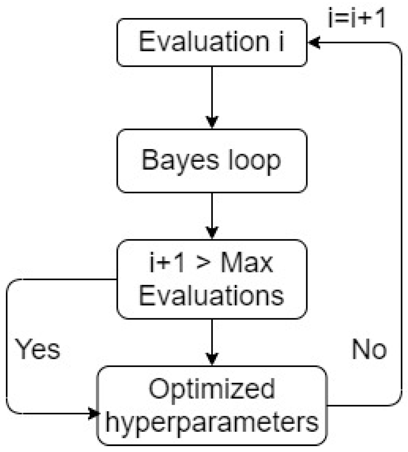
Within a set of hyperparameters selected from the imported distributions, the procedure is conducted using a Bayes loop, as follows:

• Fit the surrogate model.
• Compute the objective function and maximize the acquisition function.
• Apply the model with the intended set of hyperparameters to the data.
• Update the surrogate model to decide which set of hyperparameters from their distributions to select next.

The Bayes loop is presented in Figure 1. The procedure is presented in Figure 2 as a general schematic for SMBO. In SMBO (and Bayesian optimization as focused on in this study), the surrogate model and acquisition function are two essential key functions in the Bayesian evaluation loop. In this study, the Gaussian Process is selected as the surrogate model, albeit Tree-structured Parzen Estimator (TPE) is another comparable option [7]. Gaussian Process is a random process for a set of random variables $y_i=f\left(x_i\right), x\in R^d, i\in \left[1,N\right]$, where their joint distribution is Gaussian and formulated as:

$$p\left(f/x\right)={\rm N}(f|\mu ,K),$$

(1)

where $\mu$ is the mean function ($\mu$= $m\left(x_1\right), \dots , m\left(x_N\right))$ and $K=k\left(x_i,x_j\right)$ is a covariance (kernel) function. If $x_i \mathrm{and} x_j$ are found to be similar by Gaussian covariance function, then $f\left(x_i\right)=f\left(x_j\right)$. Knowing the training dataset $x_i$ in this case hyperparameters and their functional values $f\left(x_i\right)$, i.e., Gaussian random function, the posterior probability distribution function $f^{*}$ can be obtained, which can be used to predict a new set of hyperparameters $x_{new}$. The posterior distribution function is also gaussian and can be obtained using the gaussian conditional distribution function. To optimize the hyperparameters, the objective function $f\left(x_i\right)$ will be sampled from $j-1$ samples drawn previously, as follows:

$$x_j=argma{x}_{X}EI(x|x_{1:j-1}),$$

(2)

where EI is an acquisition function, i.e., Expected Improvement acquisition function (EI) which is widely used in the industry. For a hyperparameter set $x$, EI is defined as follows:

$$EI\left(x\right)=E[max\left(f\left(x\right)-f\left(x^{+}\right),0\right)].$$

(3)

In Equation (3), $f\left(x^{+}\right)$ is the most optimal value of the objective function (updated) for the best hyperparameter set $x^{+}$. To optimize the hyperparameter set $(x^{+})$ the Bayesian optimization algorithm is used. The nature of EI, as presented in Equation (3), always directs to select the best hyperparameter set. More advanced explanations for SMBO, Gaussian Process, EI, and a combination between Gaussian Process and EI in a Bayesian evaluation loop can be found elsewhere [8,9].

Even though Bayesian optimization has commonly been used as a search algorithm for hyperparameter optimization, it can also be used for searching an optimal ML model. However, this specific use of Bayesian optimization is limited to a few specific cases, as detailed in [7].

In this paper, Bayesian optimization is used for hyperparameter optimization and a tree-based programming tool (TPOT) is used to search for the optimal machine learning model, which is more powerful than Bayesian optimization. TPOT inherits several strengths from Genetic Programming. Both TPOT and Genetic Programming are further described below.

(c)

Genetic Programming

Genetic Programming (GP) is a pool of algorithms that closely relates to Genetic Algorithms (GA) and falls under the terminology Evolutionary Algorithms (EAs) [10]. GP was invented and has been evolved to solve general or field-specific problems in science, medicine, and engineering.

An example problem in which GP effectively excels should have two intrinsic properties. First, there should be more than one unique solution that can fit the problem, and second, although an immediate deterministic solution is unavailable, an initial set of possible solutions are known. Based on the two aforementioned properties, solutions shall be optimally and appropriately approached by the sequential selection, starting from the known initial set of possible solutions.

In GP, final solution(s) are formed using sequential reproduction processes through generations to direct an optimal fit to the problem. At a generation, a sequential reproduction starts from the selection of the best solutions (commonly defined as individuals) within the generation’s population (commonly referred to as the set of possible solutions at that generation). The selected individuals are determined using a fitting criterion (i.e., a fit function) and are further grouped as a new population for crossover. Crossover is a main reproduction operator in GP/GA [11], which processes two selected individuals (commonly named as parents), swaps portions of their structures to form new individuals (commonly named as offspring). In case the outcomes from the crossover are determined as a successful fit for the problem, the new population’s data is extracted and passed as the new generation’s population. Otherwise, the outcomes from the crossover (as exact copies from their parent individuals) are further grouped for the mutation before being passed as the new generation’s population. The mutation process is proposed to maintain diversity in a generation and expand the possibility of better results from the crossover process in the next generation. Mutation processes one selected individuals by randomly changing a portion of its structure to form a new individual.

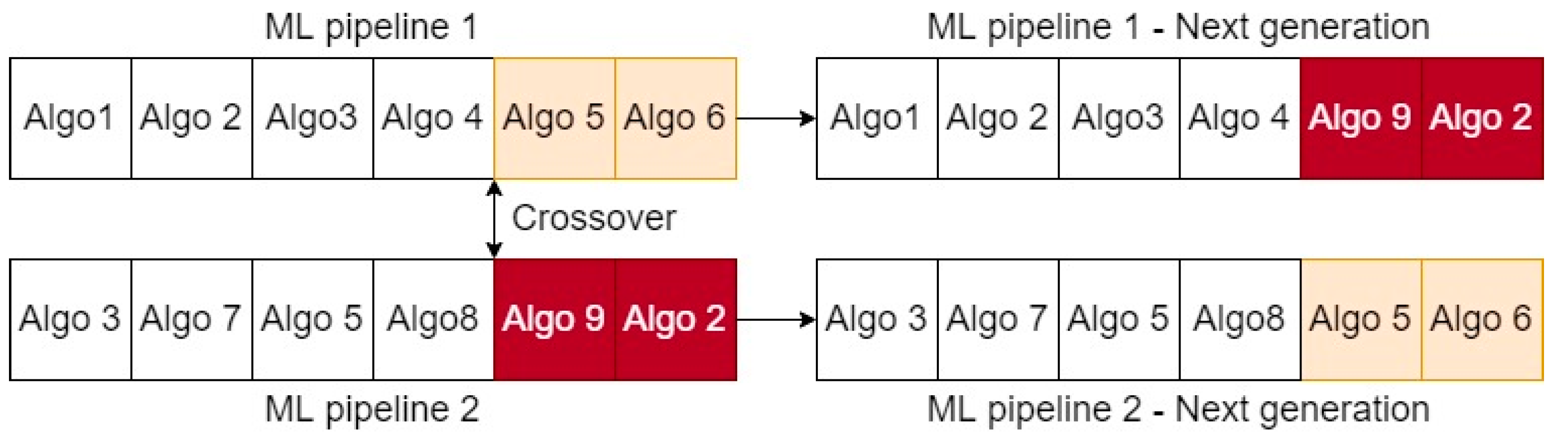
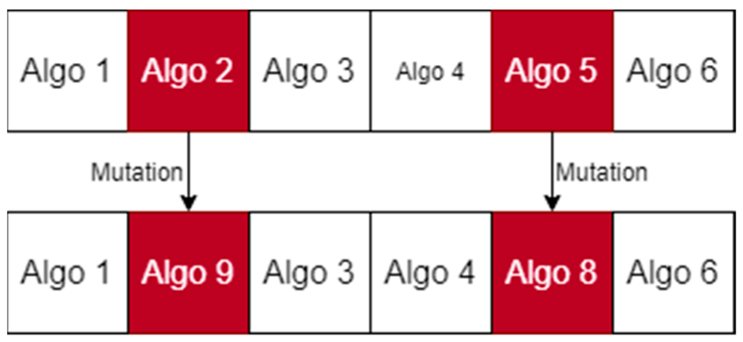
Under the context that an individual in this study is formed as a set of algorithms in sequence, crossover and mutation can be explained, as shown in Figure 3 and Figure 4. In these figures, “Algo” is an abbreviation for an algorithm in a ML pipeline (as in Figure 3 and Figure 4). In Figure 3, the crossover swaps the structure of the two individuals at the indicated double arrows (i.e., known as “single-point” crossover algorithm) and produces 2 new ML pipelines. In Figure 4, mutation chooses Algo 2 and Algo 5 in the individual’s structure and changes them to Algo 9 and Algo 8 (i.e., known as “flipping” mutation algorithm) to produce a new ML pipeline.

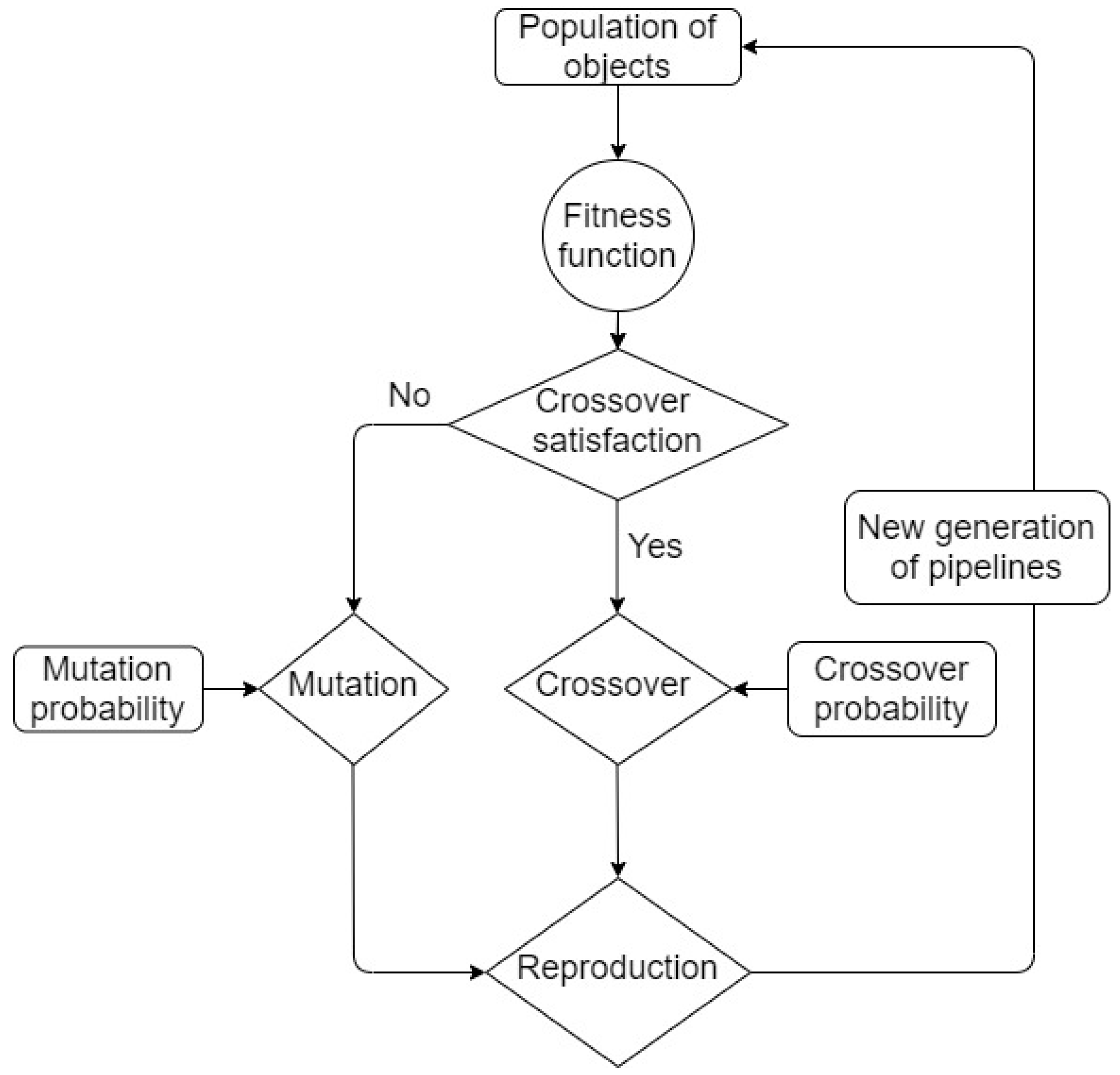
GP is inherited and functions based on the core characteristics of the biological reproduction process, including the characteristic that crossover and mutation are processed in GP with probabilistic nature. A schematic of a general GP algorithm is presented in Figure 5. Additional explanations and more details for GP/GA, crossover, and mutation can be found elsewhere [3].

(d)

Tree-based Pipeline Optimization (TPOT)

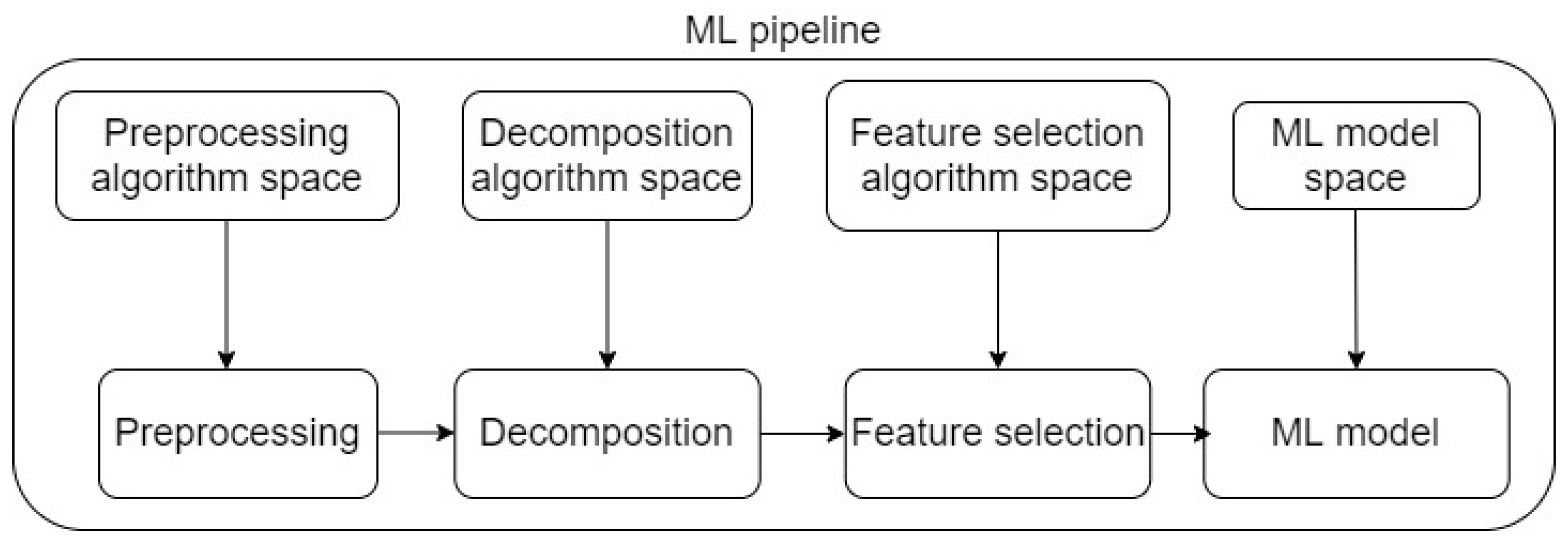
TPOT inherits characteristics from GP/GA and applies GP/GA algorithms for Automatic Machine Learning (AML) problems, which exhibit high levels of complexity and practicality for high-dimensional datasets. The foundation in TPOT is based on standard ML tasks for all ML studies, which include pre-processing, data decomposition and transformation, feature selection, and eventually modeling. This set of tasks in TPOT is defined as a machine learning pipeline. The schematic of a ML pipeline in TPOT is presented in Figure 6. Provided the fact that there exist numerous pre-processing techniques, data decomposition algorithms, feature selection techniques, and especially ML models, consequently, there exist numerous possible pipelines as suitable solutions. Additionally, a deterministic solution that is immediately optimal is challenging, as testing for all possible pipelines is impractical. Based on the nature of GP/GA, the best machine learning pipeline (as the final solution) is the one among the final generation that satisfies the optimization criteria (determined by one or more scoring metrics). In other words, TPOT implements GP to find the best machine learning pipeline through generations of searching, starting from an initial population of different pre-processing techniques, data decomposition algorithms, feature selection techniques, and especially ML models. A currently notable application of TPOT in bioinformatics can be found in [8,12].

TPOT directs the selection of the best machine learning pipeline, as follows:

• Within a generation’s population, each possible pipeline is evaluated for its fitness to the problem.
• Using the fitness results, the best pipelines are stored as a new population to process the crossover (impacted by crossover probability) and create the next potential generation of pipelines.
• All created pipelines are tested for their performance in the provided data, using pre-set scoring metric(s).
• In case the result is plausible, the created pipelines’ data is passed to the next generation.
• In case no created pipelines perform satisfactorily, a mutation is performed between the created pipelines to expand the number of pipelines (impacted by mutation probability), and data from all created pipelines (by both crossover and mutation) is passed to the next generation.
• TPOT is terminated when the stop criteria are satisfied (commonly set as the maximum number of generations reached). The representative pipeline from the final generation’s data is the most suitable machine learning pipeline for the given problem.

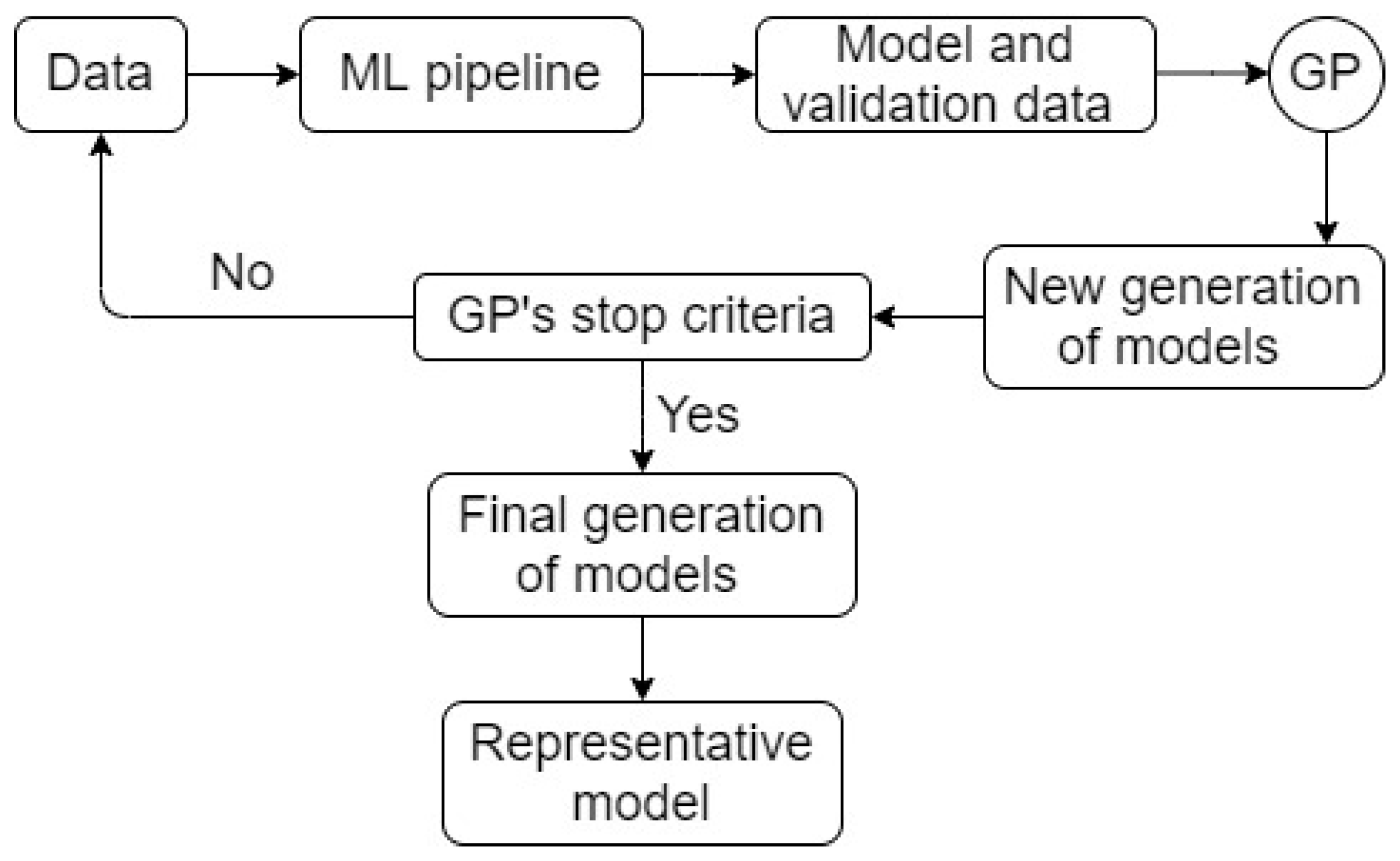
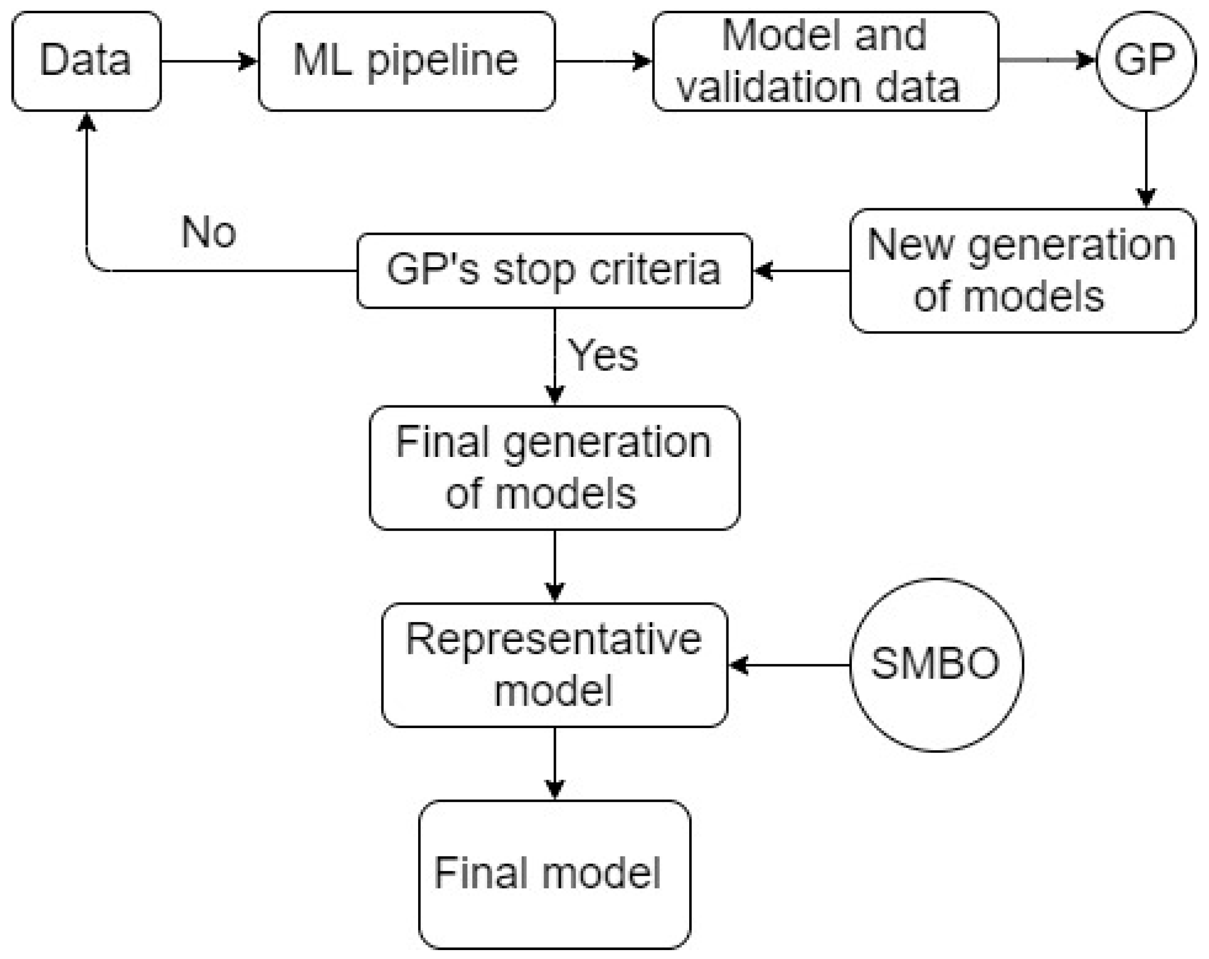
A schematic of TPOT is presented in Figure 7. TPOT was proven to perform significantly better than classical statistical analysis and manual machine learning practices [8]. Additional explanation of TPOT, its relevant development, algorithms, and especially common GP settings in TPOT can be found elsewhere [3,8].

2.3. Design of Workflows

In this paper, a new hybrid workflow is designed and tested against common practices using real filed data obtained from more than 1500 gas wells. The studied workflows are numbered in order as 1–4, and their descriptions are detailed as follows:

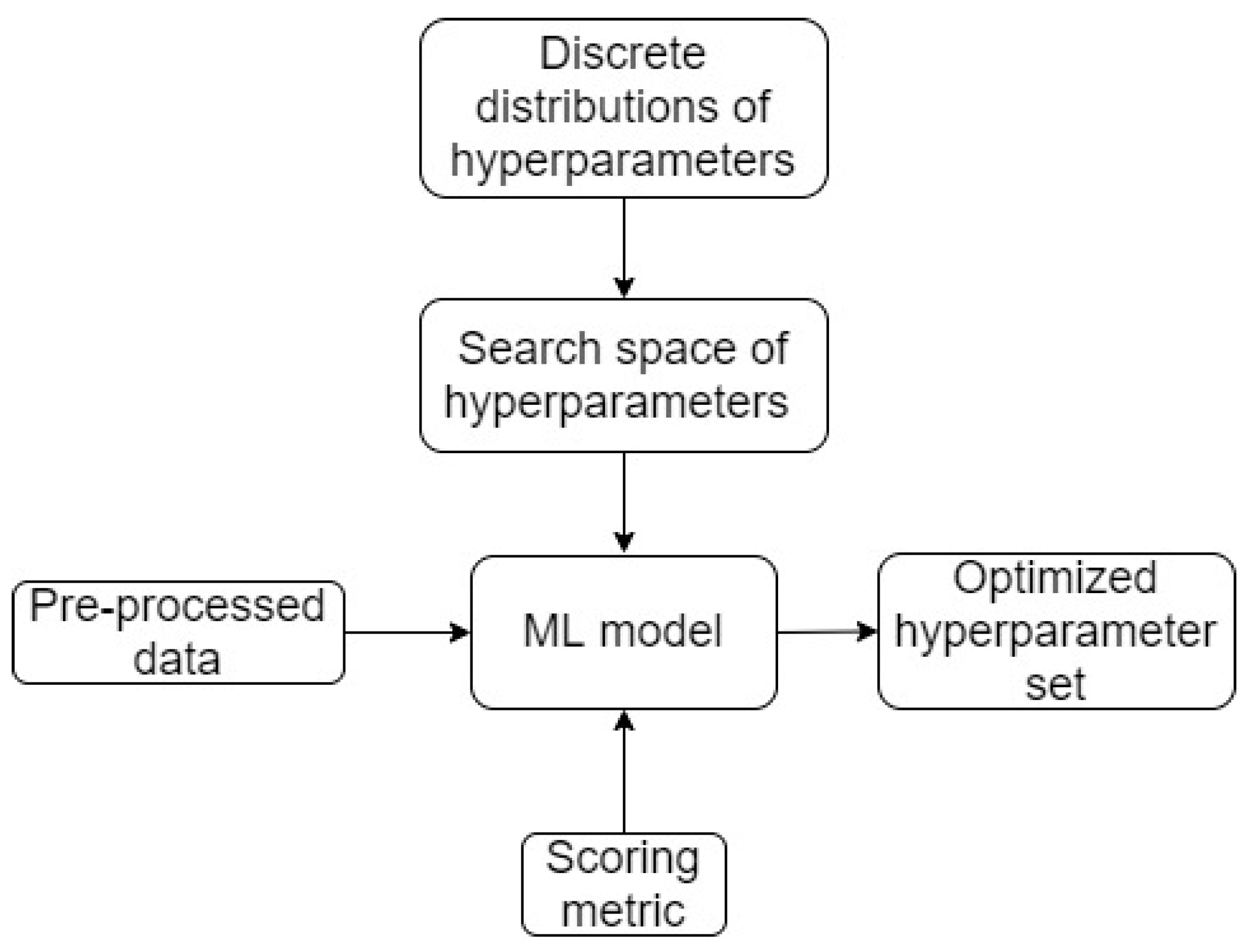
Workflow 1 (lowest level of complexity): This workflow is the most commonly used machine learning workflow, in which the model is readily pre-defined (i.e., manually selected), and the core aim is hyperparameter search [13]. The search process for hyperparameters in workflow 1 is performed using grid/random searches. A schematic of workflow 1 is presented in Figure 8.

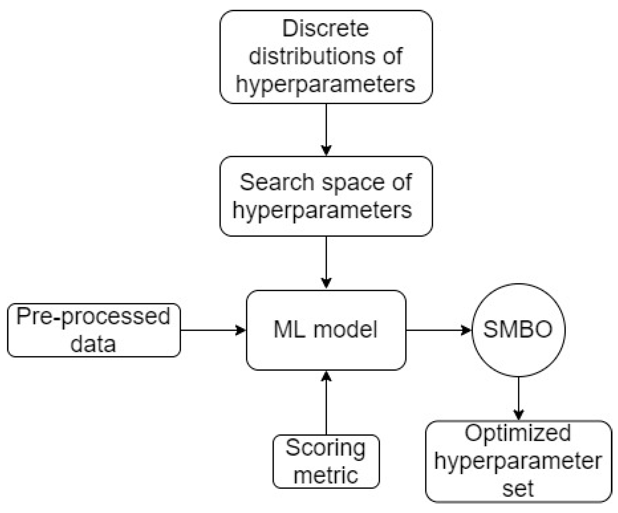
Workflow 2 (higher level of complexity compared to workflow 1): This workflow is the more advanced version of workflow 1. Its machine learning model is also manually selected and hyperparameter search remains as the central aim. However, hyperparameter search in this workflow is performed using Bayesian search and optimization. A schematic of workflow 2 is presented in Figure 9.

Workflow 3 (higher level of complexity compared to workflow 2): The central aim of this workflow is to find an optimal machine learning model using TPOT. Being inferred in the TPOT’s description, the final and optimal machine learning model is searched from a population of well-known machine learning models with various complexity levels (linear/logistic algorithms, Support Vector Machines, Random Forest, Randomized Extra Trees, Gradient Boosting, Extreme Gradient Boosting, Neural Network). Schematic of workflow 3 is readily presented in Figure 6 and Figure 7.

Workflow 4 (highest level of complexity within all workflows—a “hybrid” workflow): the central aim of this workflow is a combination of finding an optimal machine learning model and searching for its optimal hyperparameters. Workflow 4 was proposed and studied to integrate the key strengths of both TPOT and Bayes optimization. TPOT itself is a powerful set of algorithms used to focus on extracting an optimal machine learning pipeline in a modeling context, however, this tool does not focus on hyperparameter search for a machine learning model. As a result, Integration of Bayesian optimization with TPOT helps to increase the robustness of the machine learning pipeline optimization from the beginning (pre-processing) to the end (hyperparameter tuning).

For an ordered description, TPOT is initially applied in searching for an optimal ML model (similarly to workflow 3). Results from TPOT (the optimal ML model generated and its hyperparameters) are further processed through Bayesian search and optimization for searching for the best possible hyperparameters. The schematic of workflow 4 is presented in Figure 10.

2.4. Scoring Metrics for the Designed Workflows

Pearson correlation (i.e., R² correlation) and Mean Square Error (i.e., MSE) are selected as two scoring metrics to evaluate the performance of all studied workflows. These metrics are selected due to their compatibility with all the levels of complexity in the designed workflows. A minor modification of MSE to negative MSE is conducted, however, this modification merely increases seamlessly between pre-processing and modeling for a few runs and does not impact modeling evaluation.

○

Pearson correlation (R² correlation)

Pearson correlation (i.e., correlation of determination), for a sample size $n$, is computed as follows:

$$R^2\left(y,\widehat{y}\right)=1-\frac{{{\displaystyle \sum }}_{i=1}^n{\left(Y_i-{\widehat{y}}_i\right)}^2}{{{\displaystyle \sum }}_{i=1}^n{\left(Y_i-y_i\right)}^2}.$$

(4)

○

Mean Square Error (MSE)

Mean Square Error for a sample size $n$ is computed as follows:

$$MSE=\frac{1}{n-1}{{\displaystyle \sum }}_{i=1}^n{\left(y_i-{\widehat{y}}_i\right)}^2.$$

(5)

In Equations (4) and (5), $y_i$ is the known value, ${\widehat{y}}_i$ is the predicted value from the model, and $Y_i=\frac{1}{n}{\displaystyle \sum }_{i=1}^n{y}_i$ is the average value of the given data.

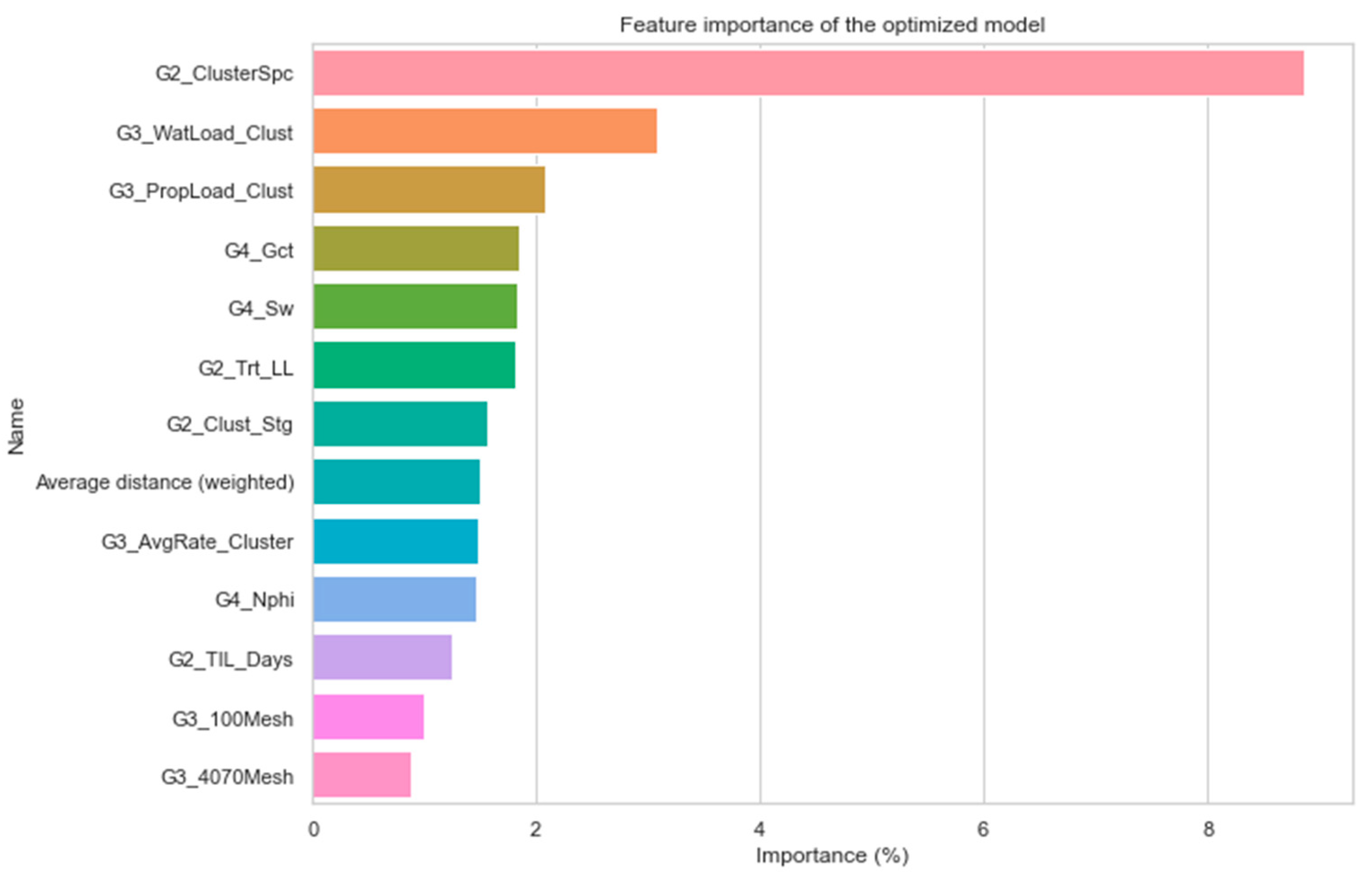
As aforementioned, workflow 4, which is a hybrid workflow between TPOT and Bayesian optimization, is further applied to real-field, high-dimensional data in the Marcellus Shale reservoir. The data contains 1567 wells and 121 features including drilling, completion, stimulation, and operation. In addition to the application of the proposed workflow to understand physical patterns in this dataset, the optimized model from the workflow is further implied in other studies for unconventional reservoir development optimization, including stimulation design, type well generation, and re-frac candidate selection. Workflow 4 exhibits superiority compared to the other studied workflows in this paper, and its superiority is detailed in the next section.

3. Analysis and Discussion

As being described, TPOT is a comprehensive and powerful set of GP algorithms, and it has been developed to be used in a variable range of problems. However, the application of TPOT for a physics-based problem requires extra attention. Figure 7 implies that any numerical and tabulated datasets can be processed through TPOT without an extra understanding of the data, as TPOT is automatically involved through the loop of generations before extraction of the final pipeline. However, a closer review of Figure 6 implies that there are processing modules within the TPOT workflow that may eliminate core and unique physical characteristics of the data. This includes pre-processing and feature selection modules. These two processing modules heavily alter the number of features and process the features in parallel. For example, the pre-processing module in TPOT may fit an imputation correlation to permeability data (without any domain intervention), and that imputation model does not reflect the observed heterogeneity of the reservoir. For another scenario, the feature-selection module may eliminate critical reservoir characteristics during its execution to reduce the number of features. Therefore, automatic use of those modules easily causes loss of physical correlations in post modeling tasks in case the alterations are permanent and were not re-analyzed before passing the processed data to GP in TPOT. In addition to that, this pre-processing workflow in TPOT is extremely time-consuming, which might heavily impact the practicality of the approach, especially when deployed in a real-time operation center (RTOC). In this study and proposed workflows, we have implemented the physical correlations between features (e.g., permeability and porosity) during data pre-processing by defining the statistical characteristics of the features and covariance (kernel) functions and re-analyzed the plausibility of the results through heatmaps after substantial alterations to the raw data such as KNN imputation. This reduced TPOT workflow is then used for this study, in which the imported data (at the beginning of the flowchart in Figure 10) is readily pre-processed and features are engineered based on domain expertise and not automatic pre-processing provided by TPOT. The exported population of machine learning pipelines, which is revolutionized through generations using GP, is merely impacted by the ML model space in Figure 10. To ensure the accuracy and robustness of our approach we have also run the full TPOT workflow where automated pre-processing is implemented within the TPOT workflow.

Table 2. Difference in pre-processing between automation and domain expertise in TPOT.

	Automation	Domain-Expertise
R2	0.721	0.702
MSE	1800	1801

shows the implication of domain expertise in pre-processing, as the raw data does not negatively impact performance compared to the native TPOT, which ensures the robustness of the approach from any human bias. The application of domain expertise in pre-processing significantly reduced the computational cost of the workflows while ensuring the accuracy of the process through R² and MSE score matrices, as shown in Table 2. Besides performance, Table 2 indicates another notable observation when the modules in the native TPOT workflow and the reduced TPOT workflow are compared. The use of human domain expertise during pre-processing is comparable to the coupled decomposition-feature selection modules in TPOT. Albeit TPOT is intrinsically designed to transform and select the optimal features, dedicated involvement of domain expertise, in this study, is proved to contribute a similar effect while ensuring the preservation of the physics of the problem.

Application of a reduced TPOT version, as in this study (driven by domain expertise as mentioned), improves the consistency of the final machine learning model through multiple runs when compared to the application of the native TPOT version and still maintains the core power of TPOT (as shown in Table 2). A reduced TPOT version reduces the number of pipelines in a population. This mitigates the flexible effects from crossover and mutation probabilities in GP, mitigates the diversity of satisfied solutions, and eventually leads to a more consistent model.

In this section, we emphasize TPOT’s applicable key strength through the designed workflows. Developing the physics-based data-driven models and eliminating the GP algorithms in workflow 4, as proposed in this study, will result in equivalent observations as in workflow 2, where the Bayesian optimization is used. In the case of small machine learning models (e.g., a 5-model search space), multiple runs using workflow 2 were observed to be capable of reproducing equivalent performance compared to a single run of workflow 4. However, in the case of complex machine learning problems, such as the one used in this study with 1567 wells and 121 features, workflow 2 will not be able to result in a model that is comparable with workflow 4, using any of the scoring matrices.

4. Result

In this paper, reservoir, drilling, completion, stimulation, and production history of 1568 wells in Marcellus Shale are collected and analyzed using four workflows, as discussed earlier. The actual field data initially consist of 121 features including measured parameters and interpreted/estimated/log from 1567 wells. The cumulative gas production after 180, 360, and 540 days are used as target parameters. To create the data-driven model with the highest accuracy, multiple data sources and formats have been integrated, and data pre-processing (i.e., imputation, standardization, cleansing, transformation, and outlier detection) is performed. Next, four different workflows are implemented to develop physics-based data-driven predictive models. The production predictions are then compared with the actual production of the blind set of wells and the performance of each workflow is quantified using R² and MSE as scoring matrices. In this paper, the results for 540 days of cumulative gas production are presented and discussed, however, similar results are obtained for 180 and 360 days of cumulative gas production as target parameters.

4.1. Final Modelling Outcomes from the Four Designed Workflows

To be able to make a one-to-one comparison, the optimal ML technique obtained using TPOT is practiced for all the workflows, and the results are presented as follows:

Workflow 1: performing workflow 1 using the Extra Randomized Tree Regressor selected using TPOT following the optimized hyperparameters obtained (min sample leaf 4, min sample split 8, number of estimators 50).

Workflow 2: Using the same model as workflow 1 implemented in workflow 2, following the optimized hyperparameters obtained (min sample leaf 4, min sample split 10, number of estimators 145).

Workflow 3: Extra Randomized Tree Regressor used in workflow 4 and the following optimum hyperparameters obtained (min sample leaf 1, min sample split 2, number of estimators 100) optimized.

Workflow 4: Extra Randomized Tree Regressor also used in our integrated workflow and the following optimum hyperparameters obtained (min sample leaf 1, min sample split 8, number of estimators 150).

4.2. Validation of the Four Designed Workflows on the Test Set

Using the two selected scoring metrics, validation of all four designed workflows (which is evaluated through the test data) is provided in

Table 3. Validation of workflows 1 and 2.

	Workflow 1	Workflow 2
R2	0.685	0.702
MSE	2832	2756

and

Table 4. Validation of workflows 3 and 4.

	Workflow 3	Workflow 4
R2	0.729	0.733
MSE	2963	2543

.

Based on Table 3 and Table 4, the use of TPOT in workflows 3 and 4 produces higher R² and lower MSE values compared to workflows 1 and 2. Based on workflow 3, the use of Bayesian optimization for hyperparameter selection as a pipeline-ended supporter to TPOT leads to a higher R² and lower MSE values in workflow 4 compared to workflow 3.

4.3. Evaluation of Marcellus Shale Gas Production Type Well

The oil and gas industry conventionally uses plots of expected well production “type curve” against “type well” of the field for quantifying the quality of the completion/operation designs and their impact on the overall NPV of the field, i.e., indexing and ranking of the wells. This ranking will then be used to obtain the best completion design practiced in the field and provides a tool for completion design optimization. The average of the field production, or P90, P50, and P10 expectations of the field production has usually been used to construct the type wells. Here, we used our new hybrid physics-based data-driven approach to generate the type well based on the total number of wells in the field. The difference between expected production and actual production is used as a benchmark to rank the wells in these techniques. For this purpose, the feature selection and ranking have been performed, as shown in Figure 11, and a statistical description of parameters used for field completion design optimization is presented in

Table 5. Field completion design optimization.

Model Parameters															Objective
	Treating Lateral Length (ft)	# Cluster per Stage	Cluster Spacing (ft)	Weterloading per Cluster (bbl/cluster)	Proppent Lading per Cluster (lbs/cluster)	100 Mesh (%)	40/70 Mesh (%)	Young’s Modulus (MMpsi)	Poisson’s Ratio	Water Saturation (%)	Porosity	Gas Content (Scf/ton)	BTU	Average Well Spacing (ft)	540 Days Cumulative Gas Production (Normalized)
Max	12323	10	119.813	2932.967	155,908.75	1	1	4.604	0.254	0.83	0.44	1674.953	1300	1501	1.621
Min	1614	2	19.834	674.916	24,039.091	0	0	2.459	0.11	0.009	0.103	0	993	438.868	0
Mean	5385.699	4.865	44.294	1559.612	67,024.683	0.585	0.333	3.116	0.181	0.117	0.229	487.909	1107.637	1039.387	0.143
Std	2070.061	0.611	16.085	446.712	21,826.928	0.242	0.218	0.429	0.029	0.098	0.035	143.885	85.478	255.413	0.099

. The parameter distributions are also available in Appendix A. Figure 11 shows that the cluster spacing has the highest impact following by water loading and proppant loading per cluster in our optimum model.

Table 6. Field completion design optimization.

Model Parameters											Objective
	# Cluster per Stage	Cluster Spacing (ft)	Water Loading per Cluster (bbl/cluster)	Proppant Loading Per Cluster (bbl/cluster)	100 Mesh (%)	40/70 Mesh (%)	30/50 Mesh (%)	Time In-Line, TIL (days)	Average Rate per Cluster	Perforation per Stage	540 Days Cumulative Gas Production (Normalized)
Type well	5	44	1569	67,374	0.58	0.34	0.06	85	19	41	1.13
P10 P50	3	60	2170	84,177	0.59	0.25	0.16	21	19	40	1.06
P50	5.0	60	1524	77,381	0.54	0.46	0	102	19.00	40	1.13
P90	5.0	30	1208	79,840	0.56	0.25	0	75	20.00	40	1.22

shows the actual type well of the field and the P10, P50, and P90 predictions of the field production using the hybrid model developed using workflow 4. For this purpose, the Monte Carlo simulation is used to sample the stimulation design parameters along with time in line. It is found that the type well of the field is very close to P50 predictions of the field, which shows great success in the completion design of the field performed by field engineers at the company. It also shows that the field average production could have been improved by 8% if shorter cluster spacing and higher proppant loading per cluster were used during the frac jobs.

5. Conclusions

Four different workflows, which exhibit different levels of complexity in investigating the optimal machine learning model and its hyperparameters, are designed to study the application of machine learning in the oil and gas industry. Levels of complexity in the workflows are underlined in the comprehensiveness of two core aspects: selecting the ML model (from random selection to genetic programming) and optimizing the hyperparameters (from random search to Bayesian optimization). Real field data in Marcellus Shale, which has 1567 wells and 121 features, is selected to study the efficacy of all the designed workflows.

Evaluation of two scoring metrics in the study emphasizes the robustness of the hybrid workflow design, which combines TPOT and Bayesian optimization. TPOT proves itself to be a powerful and directed tool for finding an optimal ML model and emphasizes the weakness of manual ML model selection. The Bayesian optimization is proved to be a solid supporter to complete the aim of TPOT. The application of the hybrid model in real field Marcellus shale confirmed the accuracy of the type well used in the field and proposed an 8% increase in total field production by decreasing the cluster spacing and increasing the proppant loading per cluster. From the evaluation in this paper, the hybrid workflow (workflow 4) is determined as a highly qualified candidate to conduct further exploration for the selected real-field, high-dimensional oil, and gas dataset such as the one available in Marcellus shale, including finding the best stimulation design in the field, designing the best type of well in the field or for a pad, and identifying potential re-frac candidates.

References

1. Belyadi, H.; Fathi, E.; Belyadi, F. Hydraulic Fracturing in Unconventional Reservoirs: Theories, Operations, and Economic Analysis, 2nd ed.; Gulf Professional Publishing: Cambridge, MA, USA, 2019. [Google Scholar]
2. Lashari, S.Z.; Borujeni, A.T.; Fathi, E.; Sun, T.; Rahmani, R.; Khazaeli, M. Drilling Performance Monitoring, and Optimization Using Artificial Intelligence Algorithms. J. Pet. Explor. Prod. Technol. 2019, 9. [Google Scholar] [CrossRef] [Green Version]
3. Bergstra, J.; Yamins, D.; Cox, D.D. Making a Science of Model Search: Hyperparameter Optimization in Hundreds of Dimensions for Vision Architectures. JMLR W CP 2013, 28, 115–123. [Google Scholar]
4. Lacoste, A.; Larochelle, H.; Laviolette, F.; Marchand, M. Sequential Model-Based Optimization. arXiv 2014, arXiv:1402.0796v1. [Google Scholar]
5. Troyanskaya, O.; Cantor, M.; Sherlock, G.; Brown, P.; Hastie, T.; Tibshirani, R.; Botstein, D.; Altman, R.B. Missing value estimation methods for DNA microarrays. Bioinformatics 2001, 17, 520–525. [Google Scholar] [CrossRef] [PubMed] [Green Version]
6. Shubert, B.O. A Sequential Method Seeking the Global Maximum of Function. 57AM J. Numer. Anal. 1972, 9, 379–388. [Google Scholar] [CrossRef]
7. Malkomes, G.; Schaff, C.; Garnett, R. Bayesian optimization for automated model selection. In Proceedings of the Neural Information Processing Systems (NIPS), Barcelona, Spain, 5–10 December 2016. [Google Scholar]
8. Mockus, J. Application of Bayesian approach to numerical methods of global and stochastic optimization. J. Glob. Optim. 1994, 4, 347–365. [Google Scholar] [CrossRef]
9. Orlenko, A.; Moore, J.H.; Orzechowski, P.; Olson, R.S.; Carins, J.; Caraballo, P.J.; Weinshilboum, R.M.; Wang, L.; Breitenstein, M.K. Considerations for automated machine learning in clinical metabolic profiling: Altered homocysteine plasma concentration associated with metformin exposure. Pac. Symp. Biocomput. 2018, 23, 460–471. [Google Scholar] [PubMed] [Green Version]
10. Sivanandam, S.N.; Deepa, A.N. Introduction to Genetic Algorithms; Springer: Berlin/Heidelberg, Germany, 2008; ISBN 978-3-540-73189-4. [Google Scholar]
11. Rasmussen, C.E.; Williams, C.K.I. Gaussian Processes for Machine Learning; MIT Press: Cambridge, MA, USA, 2006; ISBN 13 978-0-262-18253-9. [Google Scholar]
12. Olson, R.S.; Bartley, N.; Urbanowicz, R.J.; Moor, J.H. Evaluation of a Tree-based Pipeline Optimization Tool for Automating Data Science. arXiv 2016, arXiv:1603.06212v1. [Google Scholar]
13. Banzhaf, W.; Francone, F.D. Genetic Programming; Morgan Kaufman Publishers Inc.: Burlington, MA, USA, 1998. [Google Scholar]
Figure 1. Schematic of the Bayes loop.
Fuels 02 00017 g001
Figure 2. Schematic of SMBO.
Fuels 02 00017 g002
Figure 3. Demonstration of a crossover process.
Fuels 02 00017 g003
Figure 4. Demonstration of a mutation process.
Fuels 02 00017 g004
Figure 5. Schematic of genetic programming.
Fuels 02 00017 g005
Figure 6. Schematic of a ML pipeline in TPOT.
Fuels 02 00017 g006
Figure 7. Schematic of TPOT for automatic machine learning.
Fuels 02 00017 g007
Figure 8. Schematic of workflow 1.
Fuels 02 00017 g008
Figure 9. Schematic of workflow 2.
Fuels 02 00017 g009
Figure 10. Schematic for workflow 4.
Fuels 02 00017 g010
Figure 11. Feature importance of the optimized model.
Fuels 02 00017 g011