Differential Evolution in Waveform Design for Wireless Power Transfer
by
 , , , and
Pavlos Doanis
1,*,† ,
,
Achilles D. Boursianis
1,† ,
,
Julien Huillery
2,†,
Arnaud Bréard
2,†,
Yvan Duroc
2,† and
Sotirios K. Goudos
1,*,†
1
School of Physics, Aristotle University of Thessaloniki, 54124 Thessaloniki, Greece
2
Ampère UMR5005, Université de Lyon, École Centrale de Lyon, Université Claude Bernard Lyon 1, INSA Lyon, CNRS, F-69134 Ecully, France
*
Authors to whom correspondence should be addressed.
†
These authors contributed equally to this work.
Telecom 2020, 1(2), 96-113; https://0-doi-org.brum.beds.ac.uk/10.3390/telecom1020008
Submission received: 1 June 2020
/
Revised: 9 July 2020
/
Accepted: 24 July 2020
/
Published: 4 August 2020
(This article belongs to the Special Issue Modern Circuits and Systems Technologies on Communications 2020)
Abstract
:The technique of transmitting multi-tone signals in a radiative Wireless Power Transfer (WPT) system can significantly increase its end-to-end power efficiency. The optimization problem in this system is to tune the transmission according to the receiver rectenna’s nonlinear behavior and the Channel State Information (CSI). This is a non-convex problem that has been previously addressed by Sequential Convex Programming (SCP) algorithms. Nonetheless, SCP algorithms do not always attain globally optimal solutions. To this end, in this paper, we evaluate a set of Evolutionary Algorithms (EAs) with several characteristics. The performance of the optimized multi-tone transmission signals in a WPT system is assessed by means of numerical simulations, utilizing a simplified Single Input Single Output (SISO) model. From the model evaluation, we can deduce that EAs can be successfully applied to the waveform design optimization problem. Moreover, from the presented results, we can derive that EAs can obtain the optimal solutions in the tested cases.
1. Introduction
A lot of research has been recently carried out on the Internet of Things (IoT) concept. IoT is an evolutionary approach that is promising to make a great impact on everyday life and business activities. It is believed that its wide deployment will also bring economic growth, but this requires the advancement of various enabling technologies [1]. One of these technologies is Radio Frequency (RF) Wireless Power Transfer (WPT), which is used for powering up low-power devices without the need of batteries or cables [2,3,4].
In a traditional radiative WPT system, a transmitter device generates a continuous electromagnetic field, which transmits power across the medium to a receiver device (rectenna). However, the transmission of pulsed electromagnetic fields that demonstrate higher peak-to-average power ratio (PAPR) has proved to be advantageous. Pulsed wave signals are multi-tone signals that exploit the nonlinear behavior of the receiver’s rectifying circuit and increase its RF-DC conversion efficiency [5,6].
When the propagation between the transmitter and the receiver is characterized by a multipath channel function, Channel State Information (CSI) should be taken into account for the design of multi-tone signals. Towards this direction, multi-tone waveforms constructed by Time Reversal (TR) processing are proposed for WPT in [7,8]. TR waves are designed in a predetermined way, according to the CSI, and are capable of focusing on the receiver with the highest peak voltage. Consequently, they exploit both the multipath propagation channel and the nonlinear behavior of the receiver’s rectifier. The same waveform design technique was proposed in [9,10] as an Adaptive Matched Filter technique and Frequency-Maximal Ratio Transmission technique, respectively.
Another advancement in waveform design for WPT is the optimization of multi-tone waveforms according to an objective function. This function incorporates both the CSI and the rectifier’s nonlinear behavior through the analytical models of a WPT system and a simple rectenna introduced in [9]. It has been verified by numerical simulations that the transmission of these waveforms is the most efficient way to transfer power wirelessly [9]. An improvement of the objective function was proposed in [10] for the same optimization problem. The authors in both of these publications denoted that the non-convex nature of the problem is the cause of obtaining non-guaranteed globally optimal solutions by the proposed Sequential Convex Programming (SCP) methods. Many works utilizing the basic framework of [9] for waveform optimization have been published. Experimental verification of the observations made in [9] is provided in [11,12]. Low complexity optimization methods are proposed in [10,13,14]. An extension of the analytical model for application in wirelessly powered backscatter communications is introduced in [15]. In such systems, the Signal to Noise Ratio (SNR) value of the backscattered signal is equally important and is taken into consideration by adding one more constraint to the problem. The model is further extended by considering multi-tone waveforms with modulated carriers and adding a constraint to ensure a minimum rate of information transfer [16]. The waveform optimization problem has been examined for different types of systems like Single Input Single Output (SISO) in [9,10,15], Multiple Input Single Output (MISO) in [9,12,13,16], multiple users MISO in [9,13], Multiple Input Multiple Output (MIMO) in [9] and multi-receiver SISO in [17].
In artificial intelligence, Evolutionary Algorithm (EA) is a subset of evolutionary computation, i.e., a population-based metaheuristic optimization algorithm. EAs are commonly used in real-world problems and are capable of tracking the global optimum in challenging objective functions. They are equipped with mechanisms inspired by biological evolution, such as mutation, crossover, and selection, to adapt the search to the objective function’s landscape and, at the same time, to prevent convergence to a local optimum. EAs have a stochastic direct-search nature; thus they cannot ensure globally optimal solutions. However, there are many different algorithms available and each of them is suitable for different types of optimization problems.
One of the most widely known evolutionary algorithms is Differential Evolution (DE) [18]. The legacy scheme of DE algorithm is controlled by several parameters. The optimal values of these parameters differ from problem to problem and even from one stage of the search process to another [19]. Tuning DE’s control parameters before its application to a specific problem is an important and time-consuming task. As a result, the overall performance of this algorithm is highly engaged to the values of the control parameters. Researchers have put a lot of effort to develop algorithms that automatically adapt these control parameters during the search process. Two of the algorithms that have been proposed towards this direction are Composite Differential Evolution (CoDE) [20] and Success History based Adaptive DE with Linear population size reduction (L-SHADE) [21]. On the other hand, Jaya [22] is a well-promising algorithm for different types of optimization problems, since it does not have any algorithm-specific control parameters to be tuned.
Considering all the above, the optimization of the transmitted waveforms, based on a simple rectenna model and the channel state information is a promising technique to improve the overall power transfer efficiency in any WPT system. The objective of this paper is to apply various DE algorithms (DE, CoDE, L-SHADE) and the Jaya algorithm to optimize the waveform design of a WPT system and to assess the performance of the selected algorithms compared to the SCP-QCLP (Quadratically Constrained Linear Programming) method used in [10].
The novelty of this work lies in the examination of feasibility to apply various DE and Jaya algorithms in this optimization problem. To this end, there is a detailed description of the mechanisms that need to be incorporated into these algorithms for their successful implementation. These mechanisms concern the enforcement of boundary constraints. Also, a rigorous comparison between the examined algorithms is presented, taking into account not only their ability to track the optimal value of the objective function, but also their convergence speed for the tested cases.
The paper is organized as follows. In Section 2, we describe the WPT system model, including the structure of the multi-tone waveforms, the propagation channels, the rectenna circuit model, and the selected objective function. Section 3 depicts the tested EAs and the modifications needed for their application in this optimization problem. Finally, In Section 4 and Section 5, we outline the derived results and the conclusions of the paper, accordingly.
2. Wireless Power Transfer System Model
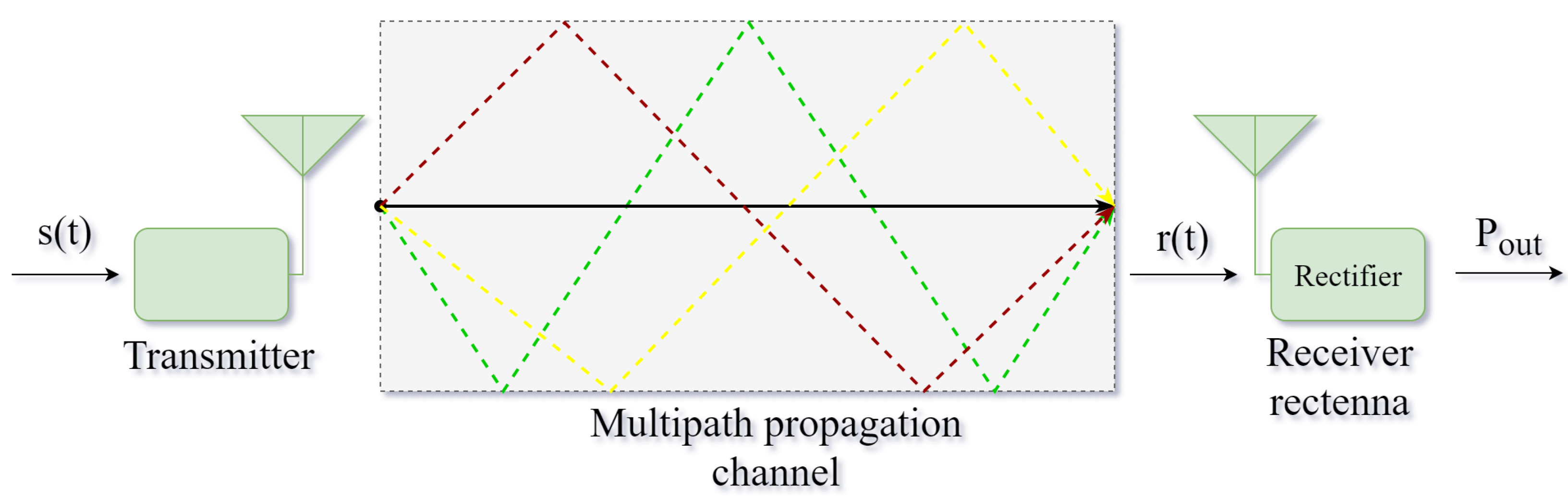
We consider a Single Input Single Output (SISO) WPT system model. This model corresponds to the simplest utilized WPT system, consisting of a transmitter, a multipath propagation channel, and a receiver rectenna (Figure 1). The wireless transfer of the power is obtained by generating and transmitting an RF signal which, after propagating across the medium, is received and rectified by the receiver rectenna (rectifier + antenna) to supply an electrical load. Hence, the objective is to design a waveform , such that the DC power at the output of the rectenna () is maximized.
2.1. Waveforms Structure
The waveform signals that have been utilized in this paper incorporate multiple sub-carriers evenly-spaced in the frequency domain. These signals are pulsed waves of a periodic form with a pulse period of , considering that the frequency space between two adjacent tones is . Each transmitted signal can be expressed in the time domain by:
where n is a positive integer, is the total number of sub-carriers, and are the amplitude in Volts, phase in radians, and frequency in Hz, of the th sub-carrier respectively. We organize the values in vectors of the following form:
According to Parseval’s theorem, if is the Fourier transform of , then the average power of in Watts can be calculated as:
The definition of the waveform’s central frequency (), bandwidth (B), and pulse period () determines the total number of sub-carriers and the associated frequencies of the signal. The minimum and maximum frequency tones in the spectrum are limited by and , accordingly. The resulted frequencies of the sub-carriers correspond to the multiples of in the interval .
To compute the received signal at the input of the rectenna, the frequency response function of the propagation across the medium is required. For a selected frequency , this can be expressed by:
where is the amplitude and is the phase of the propagation channel’s frequency response, respectively. These values can be also organized in vectors and accordingly. If we presume that the propagation channel is linear time-invariant, the incident wave at the input of the rectenna is given by:
2.2. Propagation Channels
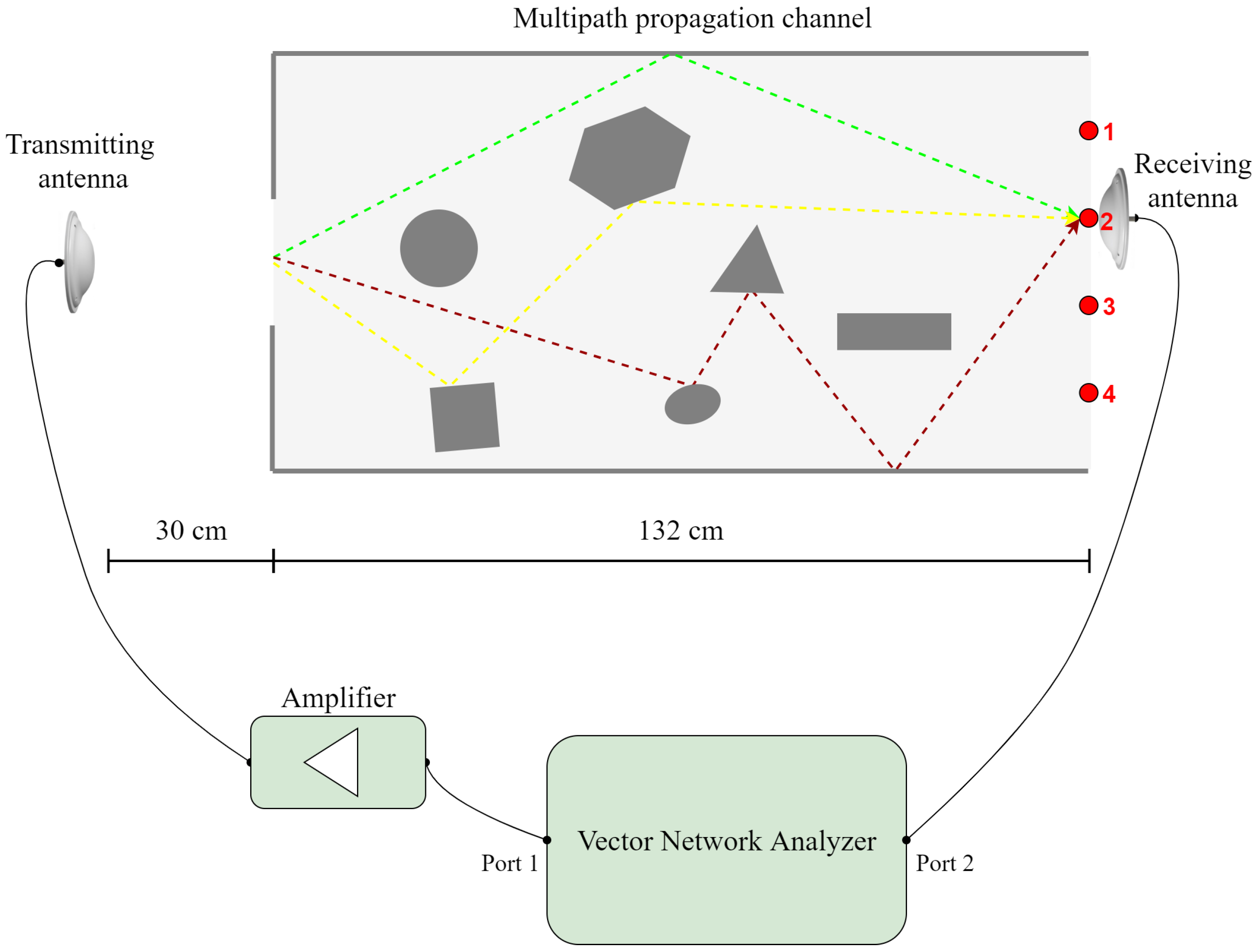
A realistic testbed of the propagation channel was fabricated in a laboratory. Since the use of CSI is more practical in a multipath propagation environment, we developed complex channels by placing a rectangular box of highly reflective surfaces and various metal obstacles between the transmitter and the receiver. A set of VNA measurements were conducted to characterize four different propagation channels, based on the four different sites of the receiver antenna, respectively (Figure 2). The obtained data by the VNA measurements were utilized to compute and depending on the waveform characteristics.
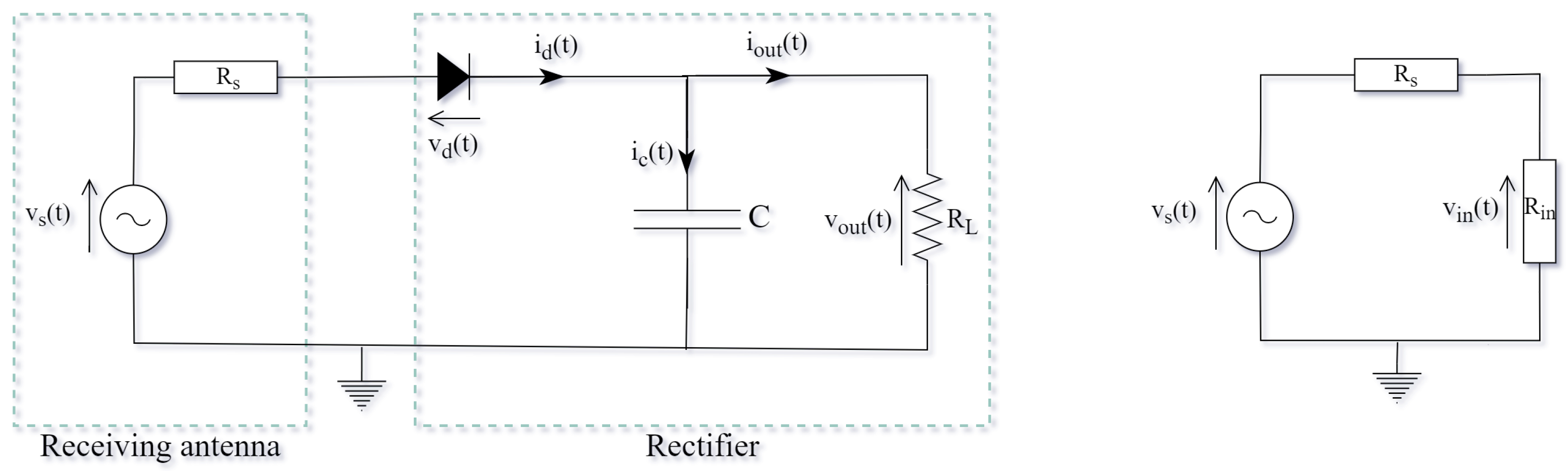
2.3. Rectenna Model
The utilized rectenna model [9,10] is depicted in Figure 3. It comprises an antenna, a single diode rectifier, and a load. The receiver antenna model also includes a voltage source and a series impedance (). The rectifier’s input impedance , as well as its input voltage is also depicted in Figure 3. In order to simplify the rectenna model, a lossless antenna and a perfect matching between the antenna and the rectifier () is considered. Moreover, the antenna noise and the diode’s series resistance are omitted. The value of the load is set to and the value of the capacitance C is equal to , resulting in a mitigation of the output fluctuation .
2.4. Objective Function
The optimization problem in hand is to design a waveform (find the corresponding and ) that maximizes the DC power delivered to the load , for a specific constraint in the average power of the designed waveform. For this problem, we apply the objective function that is utilized in [10], which is based on Kirchhoff’s circuit laws of the equivalent circuit depicted in Figure 3. The assumption of a lossless antenna, perfect matching between the antenna and the rectifier, ideal diode and negligible fluctuation of the output voltage, led to a tractable nonlinear rectenna model and made the derivation of the objective function possible [9,10]. According to [10], the formulation of the objective function can be expressed as:
which is subject to:
Based on [10], the maximization of (6) with respect to (7) maximizes the DC power delivered to the load. In (6), we set as the ideality factor of the diode and mV its thermal voltage. Also, we denote as in (7), the power constraint imposed on the designed waveform in Watts.
For the numerical computation of the integral in (6), we apply the 2-point Newton-Cotes formula [10]. To this end, we set the sampling frequency at . Considering that the sampling period is given by , the number of sub-intervals by , and Q is rounded to the nearest integer that is , (6) derives to:
The optimal selection of the phases in the transmitted signal are defined as [9]. Consequently, if we choose a specific propagation channel and a set of , B, and values, the optimization problem confines to obtain the optimal value of the vector of amplitudes that maximizes (8) with respect to the constraint in (7).
3. Evolutionary Algorithms
In a typical EA like DE, an initial random population of candidate solutions to the underlying optimization problem is evolved by applying various mathematical operators to the population’s individuals. Then, the generated solutions that demonstrate better fitness to their predecessors substitute them. The same procedure of generating new solutions and performing selection is repeated until a stopping criterion is fulfilled. The fittest individual that has survived through this process is the proposed solution to the optimization problem.
3.1. Differential Evolution
The iterations in DE algorithm are called generations (g) and the termination criterion can be set by selecting a maximum number of generations (). Alternatively, the termination criterion can be a maximum number of objective function evaluations (). The parameter vectors are called population vectors or individuals and are denoted by , where and . is called population size and it is one of the three control parameters of DE. Each vector consists of D elements that correspond to the decision variables of the optimization problem and are denoted by , where . Consequently, the dimensionality of the optimization problem is D. The population vectors in generation g are usually organized in a population matrix denoted by , which is given in (9).
The first step in DE algorithm is the initialization of NP individuals. The population vectors of the first generation are initialized randomly inside the feasible search space. Consequently, when the decision variables are subject to some constraints, these constraints should be taken into account. After the initialization phase, the algorithm enters the main loop, which consists of three different operations called mutation, crossover, and selection.
Mutation is the operation that generates mutant vectors. A mutant vector is created by perturbing one of the population vectors with the weighted difference of two others. In this way, DE exploits information from different individuals to direct the search. During mutation, each serves once as a target vector and a corresponding mutant vector is generated by:
where is called the base vector. In the classic DE version it is . Indices , and are randomly chosen every time a mutant vector is generated, under the condition that and . The scale factor (SF), denoted by F, is one of the control parameters of DE. It is always and while there is no upper limit, it is rarely [23]. We should note that (10) describes the mutation strategy in the classic version of DE, but many other different mutation strategies have been introduced in the literature.
Crossover is the operation responsible for the diversity enhancement of the population. During crossover, a new trial vector is generated for each target vector by combining some parameters of with some parameters of . This operation is controlled by a control parameter called Crossover Rate (), which may take values in the range . For the generation of a trial vector, a random number in the range is generated for each j. If this number is smaller than or equal to , the trial vector inherits its th parameter from the corresponding mutant vector, otherwise, it retains the th parameter of the target vector. Moreover, a random index is generated for each i and the new trial vector inherits its parameter from the corresponding mutant vector. This is to ensure that takes at least one element from . The crossover operation is described by:
At this point, we should note that various other crossover strategies have been also introduced in the literature.
Selection is the operation of choosing between a trial vector and the corresponding target vector. The chosen vector “survives” and continues in the next generation. The selection process is very simple in DE as the vector with the lowest fitness value will survive in a minimization problem or the vector with the largest fitness value will survive in a maximization problem. For a maximization problem, the selection operation is described by:
3.2. CoDE, L-SHADE, Jaya Algorithms
In this subsection, we are going to highlight the most important characteristics of CoDE, L-SHADE, and Jaya. We are not going to give a full description of the algorithms since their basic structure is similar to DE.
CoDE is an algorithm that is based on DE and utilizes the distinct attributes of different trial vector generation strategies and control parameter values. The term trial vector generation strategy refers to the selected mutation and crossover strategies. The authors in [20] utilized other researchers’ experiences of applying the DE algorithm in various problems to choose three trial vector generation strategies and three pairs of control parameter values that demonstrate distinct advantages. Each of them is suitable for different kinds of problems and different stages of the optimization process. The novelty in CoDE is that each one of the trial vector generation strategies is combined randomly with one of the pairs to produce three different trial vectors for each target vector. The three trial vectors compete with each other before competing with the target vector. This gives CoDE its adaptive capabilities and enables its effectiveness for a variety of optimization problems. One may say that CoDE uses adaptive control both for the control parameters and the trial vector generation strategies. The only control parameter value that needs to be adjusted is the population size.
L-SHADE is also based on the DE algorithm and it automatically adapts its control parameter values during the search process. These values, which differ between individuals, are indicated as , , and are adapted according to the control parameter values of the trial vectors that have successfully survived selection in past generations. L-SHADE features a modified mutation scheme that directs the population towards the top individuals, where . Also, an optional external archive contains former target vectors that have failed to survive selection and they are used in a way that enhances the diversity of the current population. Finally, L-SHADE incorporates a feature called Linear Population Size Reduction (LPSR), meaning that the population size is continuously reduced from generation to generation according to a linear function. Hence, L-SHADE automatically adjusts not only the , control parameters, but the population size as well. The control parameters that need to be provided in L-SHADE are the mutation scheme parameter (p), the size of the external archive (A), the size of the historical memory (H), the initial population size (), and the final population size ().
Jaya is not classified to a DE variant; nonetheless it is also a population based heuristic algorithm. It has only one mechanism for perturbing the population vectors and generating new ones. The basic concept is that the generated solutions move towards the individual with the best fitness and away from the one with the worst. Jaya is a very simple algorithm and its only control parameter is the population size.
3.3. Modifications for Application in Waveform Design
Here we describe the necessary modifications made in the original versions of the algorithms to apply them in the waveform design for the WPT problem. These include the initialization of the population and the enforcement of boundary constraints.
In the optimization problem of waveform design for WPT, the population vectors of any EA coincide with the vectors, while the dimensionality of the problem is equal to the waveform’s total number of sub-carriers (). The population vectors of the first generation are initialized randomly inside the feasible solution space. According to (7), the minimum value of is 0. On the other hand, the maximum value is , considering a scenario where all the available power would be allocated in only one of the sub-carriers. Hence, each element of the population vectors initially takes a random value between 0 and . Then, the vectors that violate the transmit power constraint are normalized so that the average transmitted power for each one of them is before entering the main loop of the algorithm. Considering that each represents a vector of amplitudes , the normalization is accomplished by multiplying the invalid vectors with a term that is calculated individually for each one of them:
The invalid vectors generated during mutation and crossover operations in DE are also substituted by vectors that lie inside the feasible solution space. This process is applied in two steps right after the crossover operation in a generation basis. In the first step, the negative valued elements of each trial vector are substituted by the respective elements of the corresponding base vector multiplied by a uniformly distributed random number in the range :
The random number is generated individually for each element substitution. In the second step, the trial vectors that violate the transmit power constraint are normalized in the same way as described earlier:
Algorithm 1 summarizes the pseudocode of DE in the WPT optimization problem. The rest of the algorithms are modified and applied in the same manner.
| Algorithm 1: Pseudocode of DE in WPT problem |
|
4. Results
4.1. Application of Algorithms
In this section, several algorithms (DE, CoDE, L-SHADE, Jaya, and SCP-QCLP) are applied in the waveform design for the WPT problem. The objective is to design multi-tone signals with and . We set = 20, 40, 80, 160, 320 ns, which lead to waveforms with = 2, 4, 8, 16, 32 sub-carriers respectively. The propagation channels examined are the four channels described in Section 2.2. Consequently, 20 different cases are assessed. The power constraint in the designed waveform is set to . This choice leads to a received signal with average power that varies from to , depending on the channel and the waveform. We consider this as a reasonable choice taking into account that in [9,10] the examined transmitted signals delivered with a received signal power of and respectively. Moreover, according to [24], a received signal of to is enough to power a modern wireless low power device. We note that the power of the finally transmitted signal is higher than since the utilized propagation channels include an amplifier and antenna before its transmission. Each algorithm is applied 50 times per case. For each obtained solution , we calculate the rectified DC power using the appropriate expressions derived by the rectenna model of Figure 3 and a bisection method as described in [10]. For this calculation we set the sampling frequency at in order to increase the accuracy in the numerical computation of the integral. From the obtained data, we compute the average rectified DC power and the corresponding standard deviation over 50 runs for each algorithm.
Before the execution of each of the applied EA algorithms, the control parameter settings, as well as the termination criteria used in each case, are determined. Table 1 lists the termination criteria and the optimal control parameter values (F, ) for DE. These values are obtained by conducting a parametric study for the 5 cases of the second propagation channel, whereas the population size is set to . For the CoDE algorithm, the population size was set equal to D, except for the cases of , where it is set to . This limitation derives from the minimum required number of population vectors in CoDE, which is 6. In L-SHADE, we set the mutation scheme parameter to , the size of the external archive to , the size of the historical memory to , the initial population size to , and the final population size to . Finally, in Jaya, we set the population size to .
4.2. Performance Comparison
The average rectified DC power for the waveforms designed by the algorithms under test is listed in Table 2. We can easily derive that all algorithms yield very similar results. Considering the performance of SCP-QCLP as the reference, we will compare the other algorithms with it. In DE, we observe a maximum percentage decrease of 2.96% in channel 1 for = 320 ns. This is a slight performance deterioration that could be explained by the fact that the tuning of F and parameters was based only on the characteristics of the second propagation channel. However, taking into consideration the overall outcome, the selected values of F and give satisfactory results for all the channels under test. Jaya’s performance is just slightly deteriorated for if we take into account the maximum percentage decrease of 0.66% in channel 4. CoDE and L-SHADE generally score values of a very slight improvement in the rectified DC power compared to SCP-QCLP, with a maximum of around 0.06% in channel 4 for = 40 ns. However, this improvement is trivial and it can be attributed to the value of the termination criterion applied in SCP-QCLP mode (it was set to as in [10]).
Table 3 lists the standard deviation values of the rectified DC power over 50 runs for each algorithm as they presented in Table 2. We can easily conclude that these values are quite low compared to the corresponding average ones. Note that SCP-QCLP should normally demonstrate zero standard deviation in any of the cases since it is not a stochastic algorithm and it is developed to converge always to the same solution. However, the observed values for SCP-QCLP are not exactly zero, due to the roundoff error of floating-point arithmetic. Table 4 and Table 5 present the best and worst values of rectified DC power detected by each algorithm. We can derive that the best values are quite similar to the worst, as expected from the corresponding low standard deviation. Also, we should remark that EAs did not detect any solution in any of the cases to demonstrate more than 0.06% increase in the rectified DC power compared to SCP-QCLP.
We should point out that the SCP methods used in [9,10] make use of some techniques to transform the original non-convex objective function into a convex one that approximates the problem and can be solved iteratively until convergence. Also, in these methods, the search starts from only one point in the solution space, which could easily lead to obtaining a locally optimal solution. On the other hand, in this paper, we employ evolutionary algorithms using the original non-convex objective function. EAs initially sample randomly the solution space and utilize a population of solutions to guide the search. Furthermore, they are equipped with mechanisms, like the crossover, to enhance the population’s diversity and prevent convergence to a local optimum. However, convergence to a globally optimal solution is still not guaranteed. We should also note that the four EAs tested in this paper have different characteristics and are suitable for different types of problems. Considering all the above, the results indicate that the obtained solutions may be the globally optimal ones.
4.3. Convergence Plots
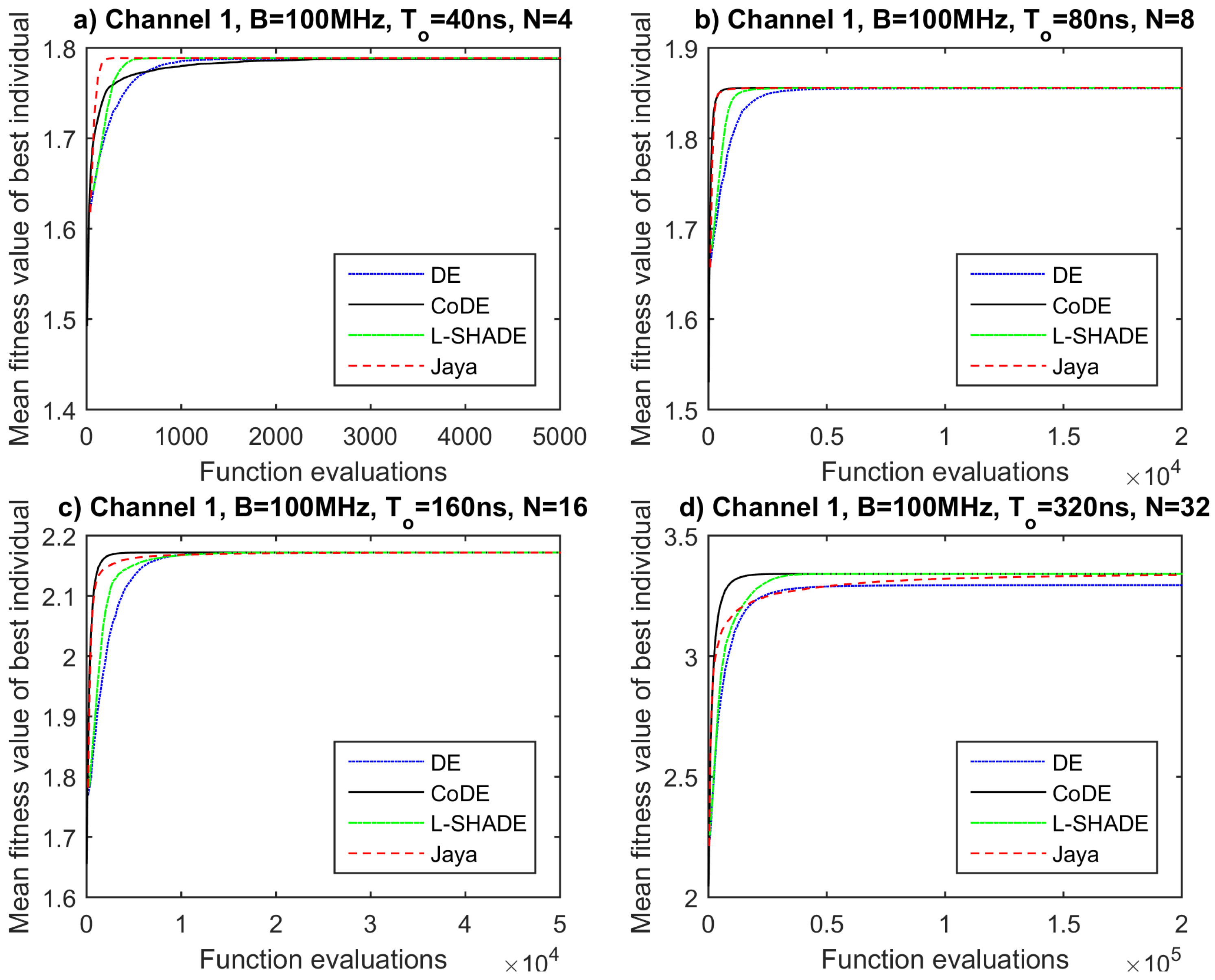
The assessment of the derived results so far has exhibited that among the tested EAs, no one stands out for yielding superior solutions. The next step for the evaluation of their performance is to check which one of them converges within a lower number of function evaluations. This can be achieved by examining the convergence plots of the algorithms in each one of the cases. These plots are generated by processing the already obtained data and depict the mean fitness value over 50 runs as a function of objective function evaluations (Figure 6, Figure 7, Figure 8 and Figure 9).
By observing the convergence plots for all channels and waveforms, we could say that CoDE algorithm converges slightly faster or at least equally fast in most of the cases compared to the other competitors. It seems that the adaptive nature of CODE makes it suitable for different problems. An exception is detected in Channel 1 for and 40 ns. The superiority of CoDE’s convergence speed is more apparent for a larger number of sub-carriers (, ). On the other hand, Jaya performs satisfactorily for and , yet poorly for and , probably due to its greedy vector generation strategy. Finally, DE and L-SHADE demonstrate quite similar behavior, as they require a larger number of function evaluations for convergence than CODE and Jaya for and , while they converge faster than Jaya and slower than CoDE for or .
5. Conclusions
In this paper, we evaluated the application of EAs in the problem of optimal waveform design for WPT systems. In detail, we applied various algorithms (DE, CoDE, L-SHADE, and Jaya) for the optimization of the transmitted multi-tone waveforms. A SISO WPT system was utilized and a multipath propagation channel was implemented. From the derived results, EAs seem to successfully obtain the optimal solutions to this non-convex problem, since all four tested algorithms converged to very similar results. However, the differences between the obtained optimal solutions from EAs and the SCP-QCLP algorithm are indiscernible. As a result, we can conclude that the objective function’s landscape for the given propagation channels is not very complicated. Consequentially, the complexity of EAs was not beneficial compared to the SCP-QCLP algorithm for the given optimization problem. Also, the results increase the confidence that the SCP approach can provide optimal waveforms despite its simplicity. Finally, CODE exhibited a slightly better convergence speed compared to the other EA algorithms.
The advantage of using EAs is that they are very flexible and can be used in conjunction with any objective function. To this end, a more realistic model of the rectifier, designed in some simulation software, could be integrated into the objective function. In that case, a charge pump circuit could be used instead of the single diode rectifier. For the given optimization problem, the disadvantage of EAs compared to SCP-QCLP is the longer execution time due to their stochastic nature.
It would be interesting to examine the application of EAs in waveform design for more complex WPT systems (more challenging objective functions). One scenario would be to examine waveform design in systems that comprise multiple transmitter antennas and/or multiple users like in [9,17]. However, in that case, it is expected that the computational time for the calculation of the objective function, and consequently the total execution time, would increase. Another scenario could be to apply EAs in systems that require the joint optimization of WPT and some other characteristic, like SNR [15] or information transfer rate [16]. That would require the modification of EAs by integrating some mechanisms for the enforcement of the additional constraints.
The optimized waveforms demonstrate high PAPR that is beneficial for the receiver rectenna’s RF to DC conversion efficiency, but not for the amplifier used in the transmission. This is because the behavior of common amplifiers is nonlinear for these types of signals. Consequently, in a real-world application, an additional constraint on PAPR should be imposed. In that case, since there is a strong limitation on the possible values, it would be interesting to examine if optimizing both and using EAs could provide some advantages.
Author Contributions
The conceptualization of the paper was done by P.D., A.D.B., J.H., Y.D. and A.B., and P.D. performed the theoretical analysis and the simulations. A.D.B., J.H., Y.D., A.B., and S.K.G. validated the theoretical analysis and simulation results. A.D.B., and S.K.G. supervised the process. All authors analyzed the results, and contributed to writing and reviewing the manuscript. All authors have read and agreed to the published version of the manuscript.
Funding
This research received no external funding.
Conflicts of Interest
The authors declare no conflict of interest.
References
- Atzori, L.; Iera, A.; Morabito, G. The Internet of Things: A survey. Comput. Netw. 2010, 54, 2787–2805. [Google Scholar] [CrossRef]
- Carvalho, N.B.; Georgiadis, A.; Costanzo, A.; Rogier, H.; Collado, A.; García, J.A.; Lucyszyn, S.; Mezzanotte, P.; Kracek, J.; Masotti, D.; et al. Wireless Power Transmission: R&D Activities Within Europe. IEEE Trans. Microw. Theory Tech. 2014, 62, 1031–1045. [Google Scholar] [CrossRef]
- Duroc, Y.; Vera, G.A. Towards Autonomous Wireless Sensors: RFID and Energy Harvesting Solutions. In Internet of Things; Mukhopadhyay, S.C., Ed.; Springer International Publishing: Cham, Switzerland, 2014; Volume 9, pp. 233–255. [Google Scholar]
- Zeng, Y.; Clerckx, B.; Zhang, R. Communications and Signals Design for Wireless Power Transmission. IEEE Trans. Commun. 2017, 65, 2264–2290. [Google Scholar] [CrossRef] [Green Version]
- Boaventura, A.S.; Carvalho, N.B. Maximizing DC power in energy harvesting circuits using multisine excitation. In Proceedings of the 2011 IEEE MTT-S International Microwave Symposium, Baltimore, MD, USA, 5–10 June 2011; pp. 1–4. [Google Scholar] [CrossRef]
- Trotter, M.S.; Griffin, J.D.; Durgin, G.D. Power-optimized waveforms for improving the range and reliability of RFID systems. In Proceedings of the 2009 IEEE International Conference on RFID, Orlando, FL, USA, 27–28 April 2009; pp. 80–87. [Google Scholar] [CrossRef]
- Ibrahim, R.; Voyer, D.; Bréard, A.; Huillery, J.; Vollaire, C.; Allard, B.; Zaatar, Y. Experiments of Time-Reversed Pulse Waves for Wireless Power Transmission in an Indoor Environment. IEEE Trans. Microw. Theory Tech. 2016, 64, 2159–2170. [Google Scholar] [CrossRef]
- Zhang, M.; Fang, C.; Doanis, P.; Huillery, J.; Breard, A.; Duroc, Y. Time-Reversal Processing for Downlink-Limited Passive UHF RFID in Pulsed Wave Mode. Antennas Wirel. Propag. Lett. 2019, 18, 2562–2566. [Google Scholar] [CrossRef]
- Clerckx, B.; Bayguzina, E. Waveform Design for Wireless Power Transfer. IEEE Trans. Signal Process. 2016, 64, 6313–6328. [Google Scholar] [CrossRef] [Green Version]
- Moghadam, M.R.V.; Zeng, Y.; Zhang, R. Waveform optimization for radio-frequency wireless power transfer: (Invited paper). In Proceedings of the 2017 IEEE 18th International Workshop on Signal Processing Advances in Wireless Communications (SPAWC), Sapporo, Japan, 3–6 July 2017; pp. 1–6. [Google Scholar] [CrossRef]
- Kim, J.; Clerckx, B.; Mitcheson, P.D. Prototyping and experimentation of a closed-loop wireless power transmission with channel acquisition and waveform optimization. In Proceedings of the 2017 IEEE Wireless Power Transfer Conference (WPTC), Taipei, Taiwan, 10–12 May 2017; pp. 1–4. [Google Scholar] [CrossRef] [Green Version]
- Kim, J.; Clerckx, B.; Mitcheson, P.D. Signal and System Design for Wireless Power Transfer: Prototype, Experiment, and Validation. arXiv 2019, arXiv:1901.01156. [Google Scholar] [CrossRef]
- Huang, Y.; Clerckx, B. Large-Scale Multiantenna Multisine Wireless Power Transfer. IEEE Trans. Signal Process. 2017, 65, 5812–5827. [Google Scholar] [CrossRef] [Green Version]
- Clerckx, B.; Bayguzina, E. Low-Complexity Adaptive Multisine Waveform Design for Wireless Power Transfer. IEEE Antennas Wirel. Propag. Lett. 2017, 16, 2207–2210. [Google Scholar] [CrossRef] [Green Version]
- Clerckx, B.; Zawawi, Z.B.; Huang, K. Wirelessly Powered Backscatter Communications: Waveform Design and SNR-Energy Tradeoff. IEEE Commun. Lett. 2017, 21, 2234–2237. [Google Scholar] [CrossRef]
- Clerckx, B. Wireless Information and Power Transfer: Nonlinearity, Waveform Design, and Rate-Energy Tradeoff. IEEE Trans. Signal Process. 2018, 66, 847–862. [Google Scholar] [CrossRef] [Green Version]
- Kim, K.; Lee, H.; Lee, J. Waveform Design for Fair Wireless Power Transfer With Multiple Energy Harvesting Devices. IEEE J. Sel. Areas Commun. 2019, 37, 34–47, Jan. [Google Scholar] [CrossRef]
- Storn, R.; Price, K. Differential Evolution—A Simple and Efficient Heuristic for global Optimization over Continuous Spaces. J. Glob. Optim. 1997, 11, 341–359. [Google Scholar] [CrossRef]
- Gämperle, R.; Mülller, S.D.; Koumoutsakos, P. A Parameter Study for Differential Evolution. In Advances in Intelligent Systems, Fuzzy Systems, Evolutionary Computation; WSEAS Press: Interlaken, Switzerland, 2002; pp. 293–298. [Google Scholar]
- Wang, Y.; Cai, Z.; Zhang, Q. Differential Evolution With Composite Trial Vector Generation Strategies and Control Parameters. IEEE Trans. Evolut. Comput. 2011, 15, 55–66. [Google Scholar] [CrossRef]
- Tanabe, R.; Fukunaga, A.S. Improving the search performance of SHADE using linear population size reduction. In Proceedings of the 2014 IEEE Congress on Evolutionary Computation (CEC), Beijing, China, 6–11 July 2014; pp. 1658–1665. [Google Scholar] [CrossRef] [Green Version]
- Venkata Rao, R. Jaya: A simple and new optimization algorithm for solving constrained and unconstrained optimization problems. Int. J. Ind. Eng. Comput. 2016, 7, 19–34. [Google Scholar] [CrossRef]
- Price, K.; Storn, R.M.; Lampinen, J.A. Differential Evolution: A Practical Approach to Global Optimization; Springer: Berlin, Germany; New York, NY, USA, 2005. [Google Scholar]
- Clerckx, B.; Costanzo, A.; Georgiadis, A.; Carvalho, N.B. Toward 1G Mobile Power Networks: RF, Signal, and System Designs to Make Smart Objects Autonomous. IEEE Microw. Mag. 2018, 19, 69–82. [Google Scholar] [CrossRef]
Figure 1.
The applied Wireless Power Transfer system model.

Figure 2.
Top view (schematic representation) of the fabricated realistic testbed for conducting VNA measurements in a complex multipath propagation channel. Details of the schematic view include the three-dimensional box interposed between the transmitter and the receiver and the highly reflective metal objects placed randomly inside the box (tinfoil has adhered to its inner walls). The sites of the receiver antenna that correspond to the propagation channels are also marked (in red color) and numbered.

Figure 3.
The equivalent circuit of the rectenna model (left) [9,10]. The same circuit depicting the equivalent impedance due to the rectifier and the load is also shown (right).

Figure 4.
(a) Waveform of the designed signal in CODE mode for propagation channel 2 and (b) corresponding signal on the rectifier’s input . The waveform’s characteristics are = 910 MHz, = 100 MHz and = 320 ns.
Figure 4.
(a) Waveform of the designed signal in CODE mode for propagation channel 2 and (b) corresponding signal on the rectifier’s input . The waveform’s characteristics are = 910 MHz, = 100 MHz and = 320 ns.

Figure 5.
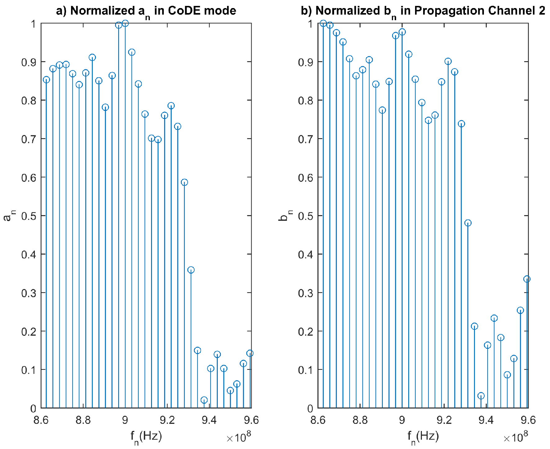
(a) Normalized amplitudes of the generated signal’s frequency tones in CoDE mode and (b) normalized amplitudes of the propagation channel 2 frequency response. The waveform’s characteristics are = 910 MHz, = 100 MHz and = 320 ns.
Figure 5.
(a) Normalized amplitudes of the generated signal’s frequency tones in CoDE mode and (b) normalized amplitudes of the propagation channel 2 frequency response. The waveform’s characteristics are = 910 MHz, = 100 MHz and = 320 ns.

Figure 6.
Convergence plots for propagation channel 1, B = 100 MHz and (a) T = 40 ns, N = 4, (b) T = 80 ns, N = 8, (c) T = 160 ns, N = 16, (d) T = 320 ns, N = 32.
Figure 6.
Convergence plots for propagation channel 1, B = 100 MHz and (a) T = 40 ns, N = 4, (b) T = 80 ns, N = 8, (c) T = 160 ns, N = 16, (d) T = 320 ns, N = 32.

Figure 7.
Convergence plots for propagation channel 2, B = 100 MHz and (a) T = 40 ns, N = 4, (b) T = 80 ns, N = 8, (c) T = 160 ns, N = 16, (d) T = 320 ns, N = 32.
Figure 7.
Convergence plots for propagation channel 2, B = 100 MHz and (a) T = 40 ns, N = 4, (b) T = 80 ns, N = 8, (c) T = 160 ns, N = 16, (d) T = 320 ns, N = 32.

Figure 8.
Convergence plots for propagation channel 3, B = 100 MHz and (a) T = 40 ns, N = 4, (b) T = 80 ns, N = 8, (c) T = 160 ns, N = 16, (d) T = 320 ns, N = 32.
Figure 8.
Convergence plots for propagation channel 3, B = 100 MHz and (a) T = 40 ns, N = 4, (b) T = 80 ns, N = 8, (c) T = 160 ns, N = 16, (d) T = 320 ns, N = 32.

Figure 9.
Convergence plots for propagation channel 4, B = 100 MHz and (a) T = 40 ns, N = 4, (b) T = 80 ns, N = 8, (c) T = 160 ns, N = 16, (d) T = 320 ns, N = 32.
Figure 9.
Convergence plots for propagation channel 4, B = 100 MHz and (a) T = 40 ns, N = 4, (b) T = 80 ns, N = 8, (c) T = 160 ns, N = 16, (d) T = 320 ns, N = 32.


Table 1.
Optimal F, values of DE algorithm and termination criteria for waveforms with = 100 MHz bandwidth.
Table 1.
Optimal F, values of DE algorithm and termination criteria for waveforms with = 100 MHz bandwidth.
| (ns) | N | (F & ) | |
|---|---|---|---|
| 20 | 2 | 500 | (1 & 0.9) |
| 40 | 4 | 5000 | (0.4 & 0.8) |
| 80 | 8 | 20,000 | (0.3 & 0.7) |
| 160 | 16 | 50,000 | (0.3 & 0.9) |
| 320 | 32 | 200,000 | (0.1 & 0.7) |
Table 2.
Summarized results (average rectified DC power in Watts) for DE, CoDE, L-SHADE, Jaya, and SCP-QCLP WPT modes. The values of the table are computed over 50 runs of each algorithm. Four different propagation channels are tested and various multi-tone waveforms with = 910 MHz, = 100 MHz and = 20, 40, 80, 160 or 320 ns are applied. The power constraint is set to = −30 dBm.
| Ch. No. | (ns) | N | DE | CODE | L-SHADE | Jaya | SCP-QCLP |
|---|---|---|---|---|---|---|---|
| 1 | 20 | 2 | 2.07835 × 10⁻⁹ | 2.07835 × 10⁻⁹ | 2.07835 × 10⁻⁹ | 2.07835 × 10⁻⁹ | 2.07835 × 10⁻⁹ |
| 1 | 40 | 4 | 1.12359 × 10⁻⁸ | 1.12212 × 10⁻⁸ | 1.12385 × 10⁻⁸ | 1.12385 × 10⁻⁸ | 1.12360 × 10⁻⁸ |
| 1 | 80 | 8 | 1.29479 × 10⁻⁸ | 1.29655 × 10⁻⁸ | 1.29655 × 10⁻⁸ | 1.29655 × 10⁻⁸ | 1.29614 × 10⁻⁸ |
| 1 | 160 | 16 | 2.21553 × 10⁻⁸ | 2.21555 × 10⁻⁸ | 2.21555 × 10⁻⁸ | 2.21535 × 10⁻⁸ | 2.21524 × 10⁻⁸ |
| 1 | 320 | 32 | 6.42805 × 10⁻⁸ | 6.62450 × 10⁻⁸ | 6.62450 × 10⁻⁸ | 6.60310 × 10⁻⁸ | 6.62428 × 10⁻⁸ |
| 2 | 20 | 2 | 1.20617 × 10⁻⁸ | 1.20617 × 10⁻⁸ | 1.20617 × 10⁻⁸ | 1.20617 × 10⁻⁸ | 1.20617 × 10⁻⁸ |
| 2 | 40 | 4 | 1.38367 × 10⁻⁸ | 1.38356 × 10⁻⁸ | 1.38367 × 10⁻⁸ | 1.38367 × 10⁻⁸ | 1.38289 × 10⁻⁸ |
| 2 | 80 | 8 | 1.96685 × 10⁻⁸ | 1.96685 × 10⁻⁸ | 1.96685 × 10⁻⁸ | 1.96685 × 10⁻⁸ | 1.96655 × 10⁻⁸ |
| 2 | 160 | 16 | 4.20886 × 10⁻⁸ | 4.20886 × 10⁻⁸ | 4.20886 × 10⁻⁸ | 4.20813 × 10⁻⁸ | 4.20882 × 10⁻⁸ |
| 2 | 320 | 32 | 1.76232 × 10⁻⁷ | 1.76295 × 10⁻⁷ | 1.76295 × 10⁻⁷ | 1.75677 × 10⁻⁷ | 1.76295 × 10⁻⁷ |
| 3 | 20 | 2 | 3.29904 × 10⁻⁸ | 3.29904 × 10⁻⁸ | 3.29904 × 10⁻⁸ | 3.29904 × 10⁻⁸ | 3.29903 × 10⁻⁸ |
| 3 | 40 | 4 | 3.96863 × 10⁻⁸ | 3.96863 × 10⁻⁸ | 3.96863 × 10⁻⁸ | 3.96863 × 10⁻⁸ | 3.96848 × 10⁻⁸ |
| 3 | 80 | 8 | 7.22309 × 10⁻⁸ | 7.23788 × 10⁻⁸ | 7.23788 × 10⁻⁸ | 7.23788 × 10⁻⁸ | 7.23565 × 10⁻⁸ |
| 3 | 160 | 16 | 2.34189 × 10⁻⁷ | 2.34189 × 10⁻⁷ | 2.34189 × 10⁻⁷ | 2.34118 × 10⁻⁷ | 2.34189 × 10⁻⁷ |
| 3 | 320 | 32 | 1.21622 × 10⁻⁶ | 1.21802 × 10⁻⁶ | 1.21802 × 10⁻⁶ | 1.21246 × 10⁻⁶ | 1.21802 × 10⁻⁶ |
| 4 | 20 | 2 | 2.11492 × 10⁻⁸ | 2.11492 × 10⁻⁸ | 2.11492 × 10⁻⁸ | 2.11492 × 10⁻⁸ | 2.11491 × 10⁻⁸ |
| 4 | 40 | 4 | 3.03277 × 10⁻⁸ | 3.03263 × 10⁻⁸ | 3.03277 × 10⁻⁸ | 3.03277 × 10⁻⁸ | 3.03080 × 10⁻⁸ |
| 4 | 80 | 8 | 8.17112 × 10⁻⁸ | 8.18408 × 10⁻⁸ | 8.18408 × 10⁻⁸ | 8.18408 × 10⁻⁸ | 8.18222 × 10⁻⁸ |
| 4 | 160 | 16 | 2.31330 × 10⁻⁷ | 2.31330 × 10⁻⁷ | 2.31330 × 10⁻⁷ | 2.31233 × 10⁻⁷ | 2.31330 × 10⁻⁷ |
| 4 | 320 | 32 | 1.10458 × 10⁻⁶ | 1.10740 × 10⁻⁶ | 1.10740 × 10⁻⁶ | 1.10012 × 10⁻⁶ | 1.10740 × 10⁻⁶ |
Table 3.
Summarized results (standard deviation of the presented average rectified DC power in Watts of Table 2) for DE, CoDE, L-SHADE, Jaya, and SCP-QCLP WPT modes. The rest of the parameter values (runs, propagation channels, multi-tone waveforms) are equivalent to the values listed in Table 2.
| Ch. No. | (ns) | N | DE | CODE | L-SHADE | Jaya | SCP-QCLP |
|---|---|---|---|---|---|---|---|
| 1 | 20 | 2 | 2.03845 × 10⁻²³ | 3.51964 × 10⁻²¹ | 1.58721 × 10⁻²³ | 2.20533 × 10⁻²³ | 1.67116 × 10⁻²⁴ |
| 1 | 40 | 4 | 1.33885 × 10⁻¹¹ | 1.02679 × 10⁻¹⁰ | 8.85871 × 10⁻²³ | 7.86836 × 10⁻²³ | 1.50404 × 10⁻²³ |
| 1 | 80 | 8 | 4.03736 × 10⁻¹¹ | 1.13520 × 10⁻¹⁷ | 1.10534 × 10⁻²² | 1.87888 × 10⁻¹⁶ | 3.34231 × 10⁻²⁴ |
| 1 | 160 | 16 | 9.54349 × 10⁻¹³ | 1.99997 × 10⁻²² | 2.01535 × 10⁻²² | 6.63979 × 10⁻¹³ | 0.00000 × 100 |
| 1 | 320 | 32 | 6.23144 × 10⁻¹⁰ | 7.43970 × 10⁻²² | 6.99875 × 10⁻²² | 3.64317 × 10⁻¹¹ | 5.34770 × 10⁻²³ |
| 2 | 20 | 2 | 1.39288 × 10⁻²¹ | 5.64683 × 10⁻²³ | 5.48058 × 10⁻²³ | 6.03609 × 10⁻²³ | 6.68463 × 10⁻²⁴ |
| 2 | 40 | 4 | 1.76173 × 10⁻²¹ | 7.32920 × 10⁻¹² | 4.16063 × 10⁻²² | 6.74128 × 10⁻¹⁷ | 1.50404 × 10⁻²³ |
| 2 | 80 | 8 | 2.89007 × 10⁻¹⁴ | 1.32441 × 10⁻²² | 1.37417 × 10⁻²² | 1.98612 × 10⁻¹⁵ | 1.67116 × 10⁻²³ |
| 2 | 160 | 16 | 2.46364 × 10⁻¹⁸ | 4.15736 × 10⁻²² | 3.40420 × 10⁻²² | 1.86467 × 10⁻¹² | 2.00539 × 10⁻²³ |
| 2 | 320 | 32 | 8.97041 × 10⁻¹¹ | 1.76089 × 10⁻²¹ | 1.31018 × 10⁻²¹ | 1.03005 × 10⁻¹⁰ | 5.34770 × 10⁻²³ |
| 3 | 20 | 2 | 3.28580 × 10⁻¹⁴ | 3.04467 × 10⁻²² | 1.41321 × 10⁻¹⁶ | 1.22182 × 10⁻¹⁴ | 1.33693 × 10⁻²³ |
| 3 | 40 | 4 | 2.39188 × 10⁻²² | 6.34539 × 10⁻¹⁵ | 1.69030 × 10⁻²² | 5.65592 × 10⁻¹⁶ | 2.67385 × 10⁻²³ |
| 3 | 80 | 8 | 2.82678 × 10⁻¹⁰ | 1.91667 × 10⁻¹⁹ | 3.42378 × 10⁻²² | 1.22729 × 10⁻¹⁴ | 5.34770 × 10⁻²³ |
| 3 | 160 | 16 | 2.06269 × 10⁻¹² | 1.03325 × 10⁻²¹ | 1.31526 × 10⁻²¹ | 1.66107 × 10⁻¹¹ | 2.40647 × 10⁻²² |
| 3 | 320 | 32 | 1.45061 × 10⁻⁹ | 4.96156 × 10⁻²¹ | 4.22229 × 10⁻²¹ | 1.00893 × 10⁻⁹ | 1.06954 × 10⁻²¹ |
| 4 | 20 | 2 | 6.71048 × 10⁻²³ | 7.98639 × 10⁻¹⁷ | 6.73789 × 10⁻²³ | 5.96170 × 10⁻²³ | 3.34231 × 10⁻²⁴ |
| 4 | 40 | 4 | 2.68488 × 10⁻¹⁴ | 6.84354 × 10⁻¹² | 1.48820 × 10⁻²² | 2.21835 × 10⁻¹⁶ | 3.34231 × 10⁻²³ |
| 4 | 80 | 8 | 4.20335 × 10⁻¹⁰ | 4.79213 × 10⁻²² | 3.62719 × 10⁻²² | 2.50819 × 10⁻¹⁴ | 0.00000 × 100 |
| 4 | 160 | 16 | 2.84362 × 10⁻¹⁵ | 1.30842 × 10⁻²¹ | 1.00846 × 10⁻²¹ | 2.88276 × 10⁻¹¹ | 1.33693 × 10⁻²² |
| 4 | 320 | 32 | 1.88389 × 10⁻⁹ | 5.03852 × 10⁻²¹ | 4.83754 × 10⁻²¹ | 1.54016 × 10⁻⁹ | 1.06954 × 10⁻²¹ |
Table 4.
Best value of the rectified DC power in Watts detected over 50 runs for DE, CoDE, L-SHADE, Jaya, and SCP-QCLP WPT modes. Four different propagation channels were tested and multi-tone waveforms with = 910 MHz, 100 MHz and = 20, 40, 80, 160 or 320 ns. The power constraint was set to dBm.
Table 4.
Best value of the rectified DC power in Watts detected over 50 runs for DE, CoDE, L-SHADE, Jaya, and SCP-QCLP WPT modes. Four different propagation channels were tested and multi-tone waveforms with = 910 MHz, 100 MHz and = 20, 40, 80, 160 or 320 ns. The power constraint was set to dBm.
| Ch. No. | (ns) | N | DE | CODE | L-SHADE | Jaya | SCP-QCLP |
|---|---|---|---|---|---|---|---|
| 1 | 20 | 2 | 2.07835 × 10⁻⁹ | 2.07835 × 10⁻⁹ | 2.07835 × 10⁻⁹ | 2.07835 × 10⁻⁹ | 2.07835 × 10⁻⁹ |
| 1 | 40 | 4 | 1.12385 × 10⁻⁸ | 1.12385 × 10⁻⁸ | 1.12385 × 10⁻⁸ | 1.12385 × 10⁻⁸ | 1.12360 × 10⁻⁸ |
| 1 | 80 | 8 | 1.29655 × 10⁻⁸ | 1.29655 × 10⁻⁸ | 1.29655 × 10⁻⁸ | 1.29655 × 10⁻⁸ | 1.29614 × 10⁻⁸ |
| 1 | 160 | 16 | 2.21555 × 10⁻⁸ | 2.21555 × 10⁻⁸ | 2.21555 × 10⁻⁸ | 2.21546 × 10⁻⁸ | 2.21524 × 10⁻⁸ |
| 1 | 320 | 32 | 6.54631 × 10⁻⁸ | 6.62450 × 10⁻⁸ | 6.62450 × 10⁻⁸ | 6.61330 × 10⁻⁸ | 6.62428 × 10⁻⁸ |
| 2 | 20 | 2 | 1.20617 × 10⁻⁸ | 1.20617 × 10⁻⁸ | 1.20617 × 10⁻⁸ | 1.20617 × 10⁻⁸ | 1.20617 × 10⁻⁸ |
| 2 | 40 | 4 | 1.38367 × 10⁻⁸ | 1.38367 × 10⁻⁸ | 1.38367 × 10⁻⁸ | 1.38367 × 10⁻⁸ | 1.38289 × 10⁻⁸ |
| 2 | 80 | 8 | 1.96685 × 10⁻⁸ | 1.96685 × 10⁻⁸ | 1.96685 × 10⁻⁸ | 1.96685 × 10⁻⁸ | 1.96655 × 10⁻⁸ |
| 2 | 160 | 16 | 4.20886 × 10⁻⁸ | 4.20886 × 10⁻⁸ | 4.20886 × 10⁻⁸ | 4.20848 × 10⁻⁸ | 4.20882 × 10⁻⁸ |
| 2 | 320 | 32 | 1.76295 × 10⁻⁷ | 1.76295 × 10⁻⁷ | 1.76295 × 10⁻⁷ | 1.75905 × 10⁻⁷ | 1.76295 × 10⁻⁷ |
| 3 | 20 | 2 | 3.29904 × 10⁻⁸ | 3.29904 × 10⁻⁸ | 3.29904 × 10⁻⁸ | 3.29904 × 10⁻⁸ | 3.29903 × 10⁻⁸ |
| 3 | 40 | 4 | 3.96863 × 10⁻⁸ | 3.96863 × 10⁻⁸ | 3.96863 × 10⁻⁸ | 3.96863 × 10⁻⁸ | 3.96848 × 10⁻⁸ |
| 3 | 80 | 8 | 7.23788 × 10⁻⁸ | 7.23788 × 10⁻⁸ | 7.23788 × 10⁻⁸ | 7.23788 × 10⁻⁸ | 7.23565 × 10⁻⁸ |
| 3 | 160 | 16 | 2.34189 × 10⁻⁷ | 2.34189 × 10⁻⁷ | 2.34189 × 10⁻⁷ | 2.34148 × 10⁻⁷ | 2.34189 × 10⁻⁷ |
| 3 | 320 | 32 | 1.21801 × 10⁻⁶ | 1.21802 × 10⁻⁶ | 1.21802 × 10⁻⁶ | 1.21444 × 10⁻⁶ | 1.21802 × 10⁻⁶ |
| 4 | 20 | 2 | 2.11492 × 10⁻⁸ | 2.11492 × 10⁻⁸ | 2.11492 × 10⁻⁸ | 2.11492 × 10⁻⁸ | 2.11491 × 10⁻⁸ |
| 4 | 40 | 4 | 3.03277 × 10⁻⁸ | 3.03277 × 10⁻⁸ | 3.03277 × 10⁻⁸ | 3.03277 × 10⁻⁸ | 3.03080 × 10⁻⁸ |
| 4 | 80 | 8 | 8.18408 × 10⁻⁸ | 8.18408 × 10⁻⁸ | 8.18408 × 10⁻⁸ | 8.18408 × 10⁻⁸ | 8.18222 × 10⁻⁸ |
| 4 | 160 | 16 | 2.31330 × 10⁻⁷ | 2.31330 × 10⁻⁷ | 2.31330 × 10⁻⁷ | 2.31302 × 10⁻⁷ | 2.31330 × 10⁻⁷ |
| 4 | 320 | 32 | 1.10730 × 10⁻⁶ | 1.10740 × 10⁻⁶ | 1.10740 × 10⁻⁶ | 1.10277 × 10⁻⁶ | 1.10740 × 10⁻⁶ |
Table 5.
Worst value of the rectified DC power in Watts detected over 50 runs for DE, CoDE, L-SHADE, Jaya, and SCP-QCLP WPT modes. Four different propagation channels were tested and multi-tone waveforms with = 910 MHz, = 100 MHz and = 20, 40, 80, 160 or 320 ns. The power constraint was set to dBm.
Table 5.
Worst value of the rectified DC power in Watts detected over 50 runs for DE, CoDE, L-SHADE, Jaya, and SCP-QCLP WPT modes. Four different propagation channels were tested and multi-tone waveforms with = 910 MHz, = 100 MHz and = 20, 40, 80, 160 or 320 ns. The power constraint was set to dBm.
| Ch. No. | (ns) | N | DE | CODE | L-SHADE | Jaya | SCP-QCLP |
|---|---|---|---|---|---|---|---|
| 1 | 20 | 2 | 2.07835 × 10⁻⁹ | 2.07835 × 10⁻⁹ | 2.07835 × 10⁻⁹ | 2.07835 × 10⁻⁹ | 2.07835 × 10⁻⁹ |
| 1 | 40 | 4 | 1.11555 × 10⁻⁸ | 1.05200 × 10⁻⁸ | 1.12385 × 10⁻⁸ | 1.12385 × 10⁻⁸ | 1.12360 × 10⁻⁸ |
| 1 | 80 | 8 | 1.27505 × 10⁻⁸ | 1.29655 × 10⁻⁸ | 1.29655 × 10⁻⁸ | 1.29655 × 10⁻⁸ | 1.29614 × 10⁻⁸ |
| 1 | 160 | 16 | 2.21499 × 10⁻⁸ | 2.21555 × 10⁻⁸ | 2.21555 × 10⁻⁸ | 2.21518 × 10⁻⁸ | 2.21524 × 10⁻⁸ |
| 1 | 320 | 32 | 6.32045 × 10⁻⁸ | 6.62450 × 10⁻⁸ | 6.62450 × 10⁻⁸ | 6.58989 × 10⁻⁸ | 6.62428 × 10⁻⁸ |
| 2 | 20 | 2 | 1.20617 × 10⁻⁸ | 1.20617 × 10⁻⁸ | 1.20617 × 10⁻⁸ | 1.20617 × 10⁻⁸ | 1.20617 × 10⁻⁸ |
| 2 | 40 | 4 | 1.38367 × 10⁻⁸ | 1.37849 × 10⁻⁸ | 1.38367 × 10⁻⁸ | 1.38367 × 10⁻⁸ | 1.38289 × 10⁻⁸ |
| 2 | 80 | 8 | 1.96683 × 10⁻⁸ | 1.96685 × 10⁻⁸ | 1.96685 × 10⁻⁸ | 1.96685 × 10⁻⁸ | 1.96655 × 10⁻⁸ |
| 2 | 160 | 16 | 4.20886 × 10⁻⁸ | 4.20886 × 10⁻⁸ | 4.20886 × 10⁻⁸ | 4.20763 × 10⁻⁸ | 4.20882 × 10⁻⁸ |
| 2 | 320 | 32 | 1.75929 × 10⁻⁷ | 1.76295 × 10⁻⁷ | 1.76295 × 10⁻⁷ | 1.75450 × 10⁻⁷ | 1.76295 × 10⁻⁷ |
| 3 | 20 | 2 | 3.29902 × 10⁻⁸ | 3.29904 × 10⁻⁸ | 3.29904 × 10⁻⁸ | 3.29903 × 10⁻⁸ | 3.29903 × 10⁻⁸ |
| 3 | 40 | 4 | 3.96863 × 10⁻⁸ | 3.96862 × 10⁻⁸ | 3.96863 × 10⁻⁸ | 3.96863 × 10⁻⁸ | 3.96848 × 10⁻⁸ |
| 3 | 80 | 8 | 7.11523 × 10⁻⁸ | 7.23788 × 10⁻⁸ | 7.23788 × 10⁻⁸ | 7.23787 × 10⁻⁸ | 7.23565 × 10⁻⁸ |
| 3 | 160 | 16 | 2.34174 × 10⁻⁷ | 2.34189 × 10⁻⁷ | 2.34189 × 10⁻⁷ | 2.34081 × 10⁻⁷ | 2.34189 × 10⁻⁷ |
| 3 | 320 | 32 | 1.21202 × 10⁻⁶ | 1.21802 × 10⁻⁶ | 1.21802 × 10⁻⁶ | 1.20816 × 10⁻⁶ | 1.21802 × 10⁻⁶ |
| 4 | 20 | 2 | 2.11492 × 10⁻⁸ | 2.11492 × 10⁻⁸ | 2.11492 × 10⁻⁸ | 2.11492 × 10⁻⁸ | 2.11491 × 10⁻⁸ |
| 4 | 40 | 4 | 3.03275 × 10⁻⁸ | 3.02810 × 10⁻⁸ | 3.03277 × 10⁻⁸ | 3.03277 × 10⁻⁸ | 3.03080 × 10⁻⁸ |
| 4 | 80 | 8 | 7.92012 × 10⁻⁸ | 8.18408 × 10⁻⁸ | 8.18408 × 10⁻⁸ | 8.18407 × 10⁻⁸ | 8.18222 × 10⁻⁸ |
| 4 | 160 | 16 | 2.31330 × 10⁻⁷ | 2.31330 × 10⁻⁷ | 2.31330 × 10⁻⁷ | 2.31164 × 10⁻⁷ | 2.31330 × 10⁻⁷ |
| 4 | 320 | 32 | 1.09734 × 10⁻⁶ | 1.10740 × 10⁻⁶ | 1.10740 × 10⁻⁶ | 1.09666 × 10⁻⁶ | 1.10740 × 10⁻⁶ |
© 2020 by the authors. Licensee MDPI, Basel, Switzerland. This article is an open access article distributed under the terms and conditions of the Creative Commons Attribution (CC BY) license (http://creativecommons.org/licenses/by/4.0/).
Share and Cite
MDPI and ACS Style
Doanis, P.; Boursianis, A.D.; Huillery, J.; Bréard, A.; Duroc, Y.; Goudos, S.K. Differential Evolution in Waveform Design for Wireless Power Transfer. Telecom 2020, 1, 96-113. https://0-doi-org.brum.beds.ac.uk/10.3390/telecom1020008
AMA Style
Doanis P, Boursianis AD, Huillery J, Bréard A, Duroc Y, Goudos SK. Differential Evolution in Waveform Design for Wireless Power Transfer. Telecom. 2020; 1(2):96-113. https://0-doi-org.brum.beds.ac.uk/10.3390/telecom1020008
Chicago/Turabian StyleDoanis, Pavlos, Achilles D. Boursianis, Julien Huillery, Arnaud Bréard, Yvan Duroc, and Sotirios K. Goudos. 2020. "Differential Evolution in Waveform Design for Wireless Power Transfer" Telecom 1, no. 2: 96-113. https://0-doi-org.brum.beds.ac.uk/10.3390/telecom1020008