Feature Importances: A Tool to Explain Radio Propagation and Reduce Model Complexity


Radiocommunications Laboratory, Physics Department, Aristotle University of Thessaloniki, 54124 Thessaloniki, Greece
*
Author to whom correspondence should be addressed.
Telecom 2020, 1(2), 114-125; https://0-doi-org.brum.beds.ac.uk/10.3390/telecom1020009
Submission received: 18 June 2020
/
Revised: 4 August 2020
/
Accepted: 17 August 2020
/
Published: 21 August 2020
Abstract
:Machine learning models have been widely deployed to tackle the problem of radio propagation. In addition to helping in the estimation of path loss, they can also be used to better understand the details of various propagation scenarios. Our current work exploits the inherent ranking of feature importances provided by XGBoost and Random Forest as a means of indicating the contribution of the underlying propagation mechanisms. A comparison between two different transmitter antenna heights, revealing the associated propagation profiles, is made. Feature selection is then implemented, leading to models with reduced complexity, and consequently reduced training and response times, based on the previously calculated importances.
1. Introduction
Radio coverage, received power levels, and path loss are parameters of crucial importance when designing mobile communication networks. The need for fast and accurate predictions has driven the deployment of many path loss prediction models.
Artificial intelligence and machine learning have provided reliable solutions for modeling radio propagation. A wide variety of models have been deployed [1,2,3,4,5] and optimized [6,7] to produce trustworthy estimations of path loss prediction. However, these models are mostly considered to be black boxes. That is, their internal functionality and decision-making process are considered to be opaque. This situation degrades the assistance of the machine learning models, leaving a significant part of their potential unused.
Our current work examines the possibility of using two machine learning models (namely XGBoost and Random Forest) as both predictors and explainers. That is, in addition to, and in parallel with, the path loss predictions, we attempt to use the models to better explain and understand the underlying propagation mechanisms.
In this paper, two propagation scenarios for two different base station antenna heights are examined. The predictions are explained in conjunction with the respective propagation mechanisms. These mechanisms are indicated using machine learning models, specifically with their internal mechanism of ranking feature importances. It should be mentioned that the work in [8] uses Random Forest’s inherent ranking of feature importances to explain path loss between two unmanned aerial vehicles.
As stated in [9], an increased number of features does not necessarily lead to a model with better performance. This is why it has been suggested [9] that methodologies are developed to guide the procedure of feature selection. A step towards that direction is to use the ranked feature importances as a means to produce models with fewer inputs, describing the trade-off between prediction performance and model complexity.
The contributions of our work can be summarized as follows:
- ○
- Insight into the model’s behavior is gained through the association between the changes in feature importances and the emergence of different radio propagation mechanisms.
- ○
- Simpler and faster models are deployed through a feature selection procedure based on the ranked importances.
2. Propagation Mechanisms According to the Transmitter’s Height
For a given built-up environment, the arising propagation mechanisms are dictated from the transmitter’s height. More specifically, for the case of placing the transmitter well below the rooftop level, the received field (for NLOS conditions) is characterized by multiple reflected rays from building walls, in addition to diffractions from perpendicular building corners [10,11]. By comparison, when the transmitter is placed well above the rooftops, electromagnetic waves propagate above them until they are diffracted down to the receiver [11,12]. For the intermediate case, when the transmitter is placed at a height near building rooftops, a mixture of propagation mechanisms takes place. That is, neither propagation inside streets nor over-rooftop diffraction can be neglected [13]. This situation is difficult to simulate because many propagation mechanisms have to be taken into account.
From a machine learning model’s perspective, simulation of the above-mentioned mechanisms proceeds with feature engineering [14]: that is, the inputs of the model should describe those parameters of the built-up environment that have the greatest influence on the dominant propagation mechanisms. For the case of placing the transmitter well above the rooftop height, the inputs should describe the mechanism of over-rooftop diffraction [15]; this is why the position of the tallest building along the Line of Sight path near the receiver is expected to determine the level of the received power. However, when the transmitter height is reduced, the contribution of over rooftop diffraction also decreases, steadily giving rise to the mechanism of multiple reflections and the creation of an urban street canyon. A feature that could be coupled with this mechanism is that which depicts the number of buildings that obstruct the LOS path, thus producing the aforementioned reflections.
3. Problem Description and Model Used
3.1. Features and the Associated Propagation Mechanisms
The propagation environment and the 23 features that describe it were introduced in our previous research [15,16,17]. The area is formed from rectangular buildings, whose dimensions (in addition to the roads’ dimensions) are randomly distributed, corresponding to an urban area. All measurements are taken along the roads and at the crossroads of the area.
The 23 features describe the Line of Sight path (Figure 1), the area around the receiver (Figure 2), and the positions of the transmitter and the receiver, in addition to the distances between them (Figure 3).
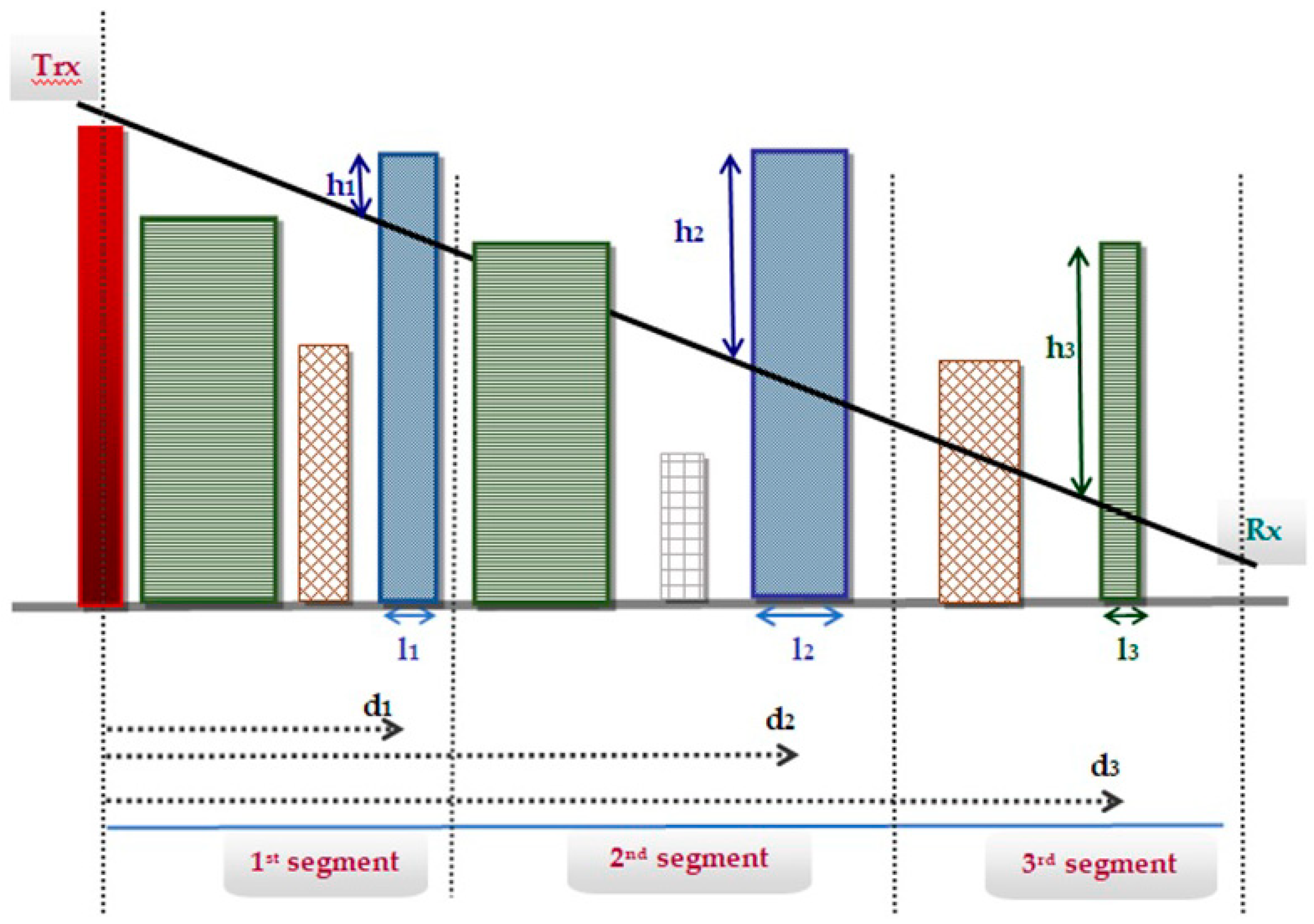
Looking closer at the group of the 10 features of the Line of Sight path, nine [18] refer to specific segments (three features for each of the three segments created). For a transmitter placed well above the rooftop, the features describing the third segment, and primarily the position of its tallest building, are expected to have the greatest influence on the power received.
The 10th feature of this group describes the whole Line of Sight path. Its value is equal to the number of buildings that obstruct the direct ray (which is equal to five for Figure 1). These buildings act as sources for the mechanism of multiple reflections. Thus, this feature is expected to have a greater impact when the height of the transmitter is reduced.
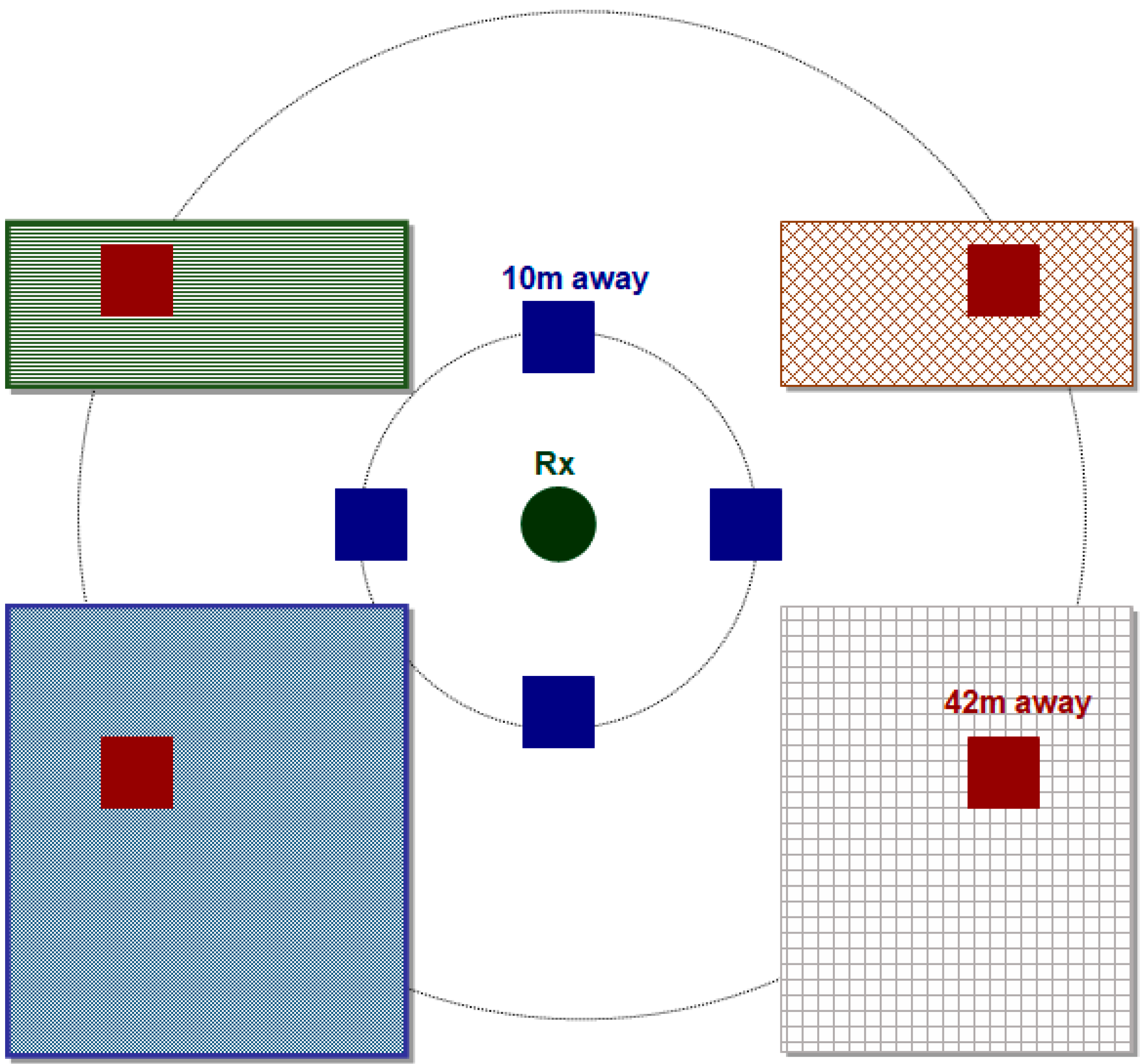
Features 11 to 18 describe the area around the receiver. As shown in Figure 2, they return the heights of the nearest buildings. If the point in question corresponds to a road, the returned value is equal to 0.
It is apparent that information regarding the map of the area is needed to calculate the values corresponding to each feature. This could either be obtained through specific databases, or through a combination of OpenStreetMap [19] (which provides the footprints of the buildings) and the open source software QGIS (which provides the heights of the buildings).
3.2. Models Used: XGBoost and Random Forest
XGBoost [20] and Random Forest [21] were implemented to make predictions based on the aforementioned features. Their performance when dealing with features of tabular data format, in addition to their built-in capability of ranking feature importances, were the reasons for choosing them.
Both models are based on the combination of regression trees. That is, both are ensemble methods, whose final predictions are based on the combination of the predictions of single regression trees. A key difference exists between them, however, in the manner in which each ensemble is constructed [22]. XGBoost utilizes the concept of boosting, whereas Random Forest relies on the concept of bagging.
According to bagging, all trees are grown in parallel, with each tree a standalone predictor of the quantity under estimation. The ensemble’s estimation is the average of the estimations of all trees. Boosting, by comparison, relies on the sequential growth of trees. Each new tree is grown with respect to the previous tree’s errors, and tries to compensate for these errors.
3.3. Relative Feature Importances in Tree-Based Models
Feature selection is a crucial element of the design of every machine learning model [23]. It can be performed based on the ranking of features, according to their contribution to the model’s predictions. A number of specific methods which calculate feature importance have been developed. An exhaustive approach towards this goal would involve first training the model according to every possible subgroup of features, and then comparing the estimation results to determine the most efficient subgroup of features. Such an approach would need a vast amount of computer resources and would also be extremely time-consuming.
Another approach, which is implemented in the current study, is one that takes advantage of the built-in ability of most tree-based models to rank features (also denoted as predictors) according to their participation in the process of node splitting during the procedure of building the regression trees.
Each node of a regression tree corresponds to one of the predictors, combined with a cutpoint (or split point) of the aforementioned predictor. The terminal nodes hold the value of the output variable. That is, for every given set of predictors’ values, a specific path through the nodes is followed, finally leading to a terminal node where the prediction is contained; that is, the tree segregates the predictor space (which is the set of all possible values for all predictors) to make its predictions. Every added node divides the predictor space further.
Node splitting can be described as a procedure in which [22] the predictor space is divided into two distinct and non-overlapping regions in such a way that the residual sum of squares is minimized. This means that all predictors, in addition to all possible cutpoint values for each predictor, are considered to perform the split. The procedure terminates when a preselected criterion (mostly referring to the tree’s maximum depth or the minimum number of training examples corresponding to a single node) is met.
Mathematically speaking, for any predictor j and any cutpoint s, the following pair of half-planes is defined:
where the notation denotes the region of the predictor space in which the observation Xj takes on a value less than s.
The values of j and s are determined such that the following quantity (residual sum of squares) is minimized:
where is the mean response for the training observations xi in the region R1(j,s) and is the mean response for the training observations xi in the region R2(j,s). The actual output for the ith input pattern is denoted yi.
It is therefore straightforward to claim that node splitting improves the tree’s predictions. The sum of the improvements over all nodes of a tree for which the splits were made according to a particular feature is the relative importance of that feature. This measure of importance is then easily generalized to the whole ensemble of trees by calculating it for each individual tree and averaging it for the total number of trees.
3.4. Metrics of the Prediction Error
The error measurement metrics reflect the distance between the actual and the predicted values. Two of the most widely used error metrics, with their definitions, are shown in the following equations:
where yi(p) is the actual path loss value, yi,mean(p) is the mean actual path loss value and yo(p) is the predicted path loss value. Ntest is the number of test patterns, while p represents the input according to which the prediction is made.
4. Numerical Results
Two collections of 34,501 simulations, corresponding to two transmitter heights (namely 35 and 30 m) were taken from a specific software application implementing the ray-tracing algorithm [24].
The area under consideration was urban, with randomly distributed dimensions of buildings and roads. The building heights ranged between 5 and 29 m, regardless of the base station’s height. We could therefore characterize the case where the transmitter height is equal to 35 m as a scenario in which the base station is placed well above the rooftops (because even the tallest building would be 6 m below the transmitter). This assumption does not fully hold true when placing the transmitter at 30 m because buildings would exist that have only a 1 m difference in height with the placement of the transmitter, therefore leading to a situation where the base station is placed at a height close to that of the building rooftops.
Both sets of simulations were split into a training set consisting of 80%, and the corresponding testing set comprised 20% of the simulations.
4.1. Path Loss Predictions for Both Models and Transmitter Heights
Table 2 presents the MAE and R2 values for both models and transmitter heights. Each model was constructed with 700 trees.
It is clear that the prediction is more precise at the 35 m case. Moreover, XGBoost leads to better results than Random Forest for both transmitter heights.
4.2. Feature Importances When the Transmitter is at 30 m
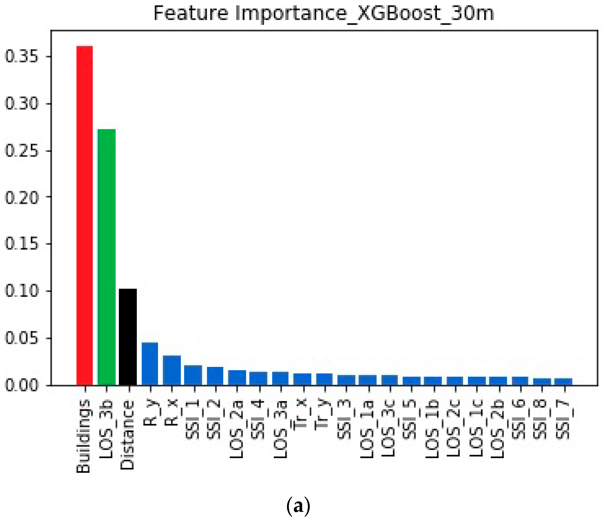
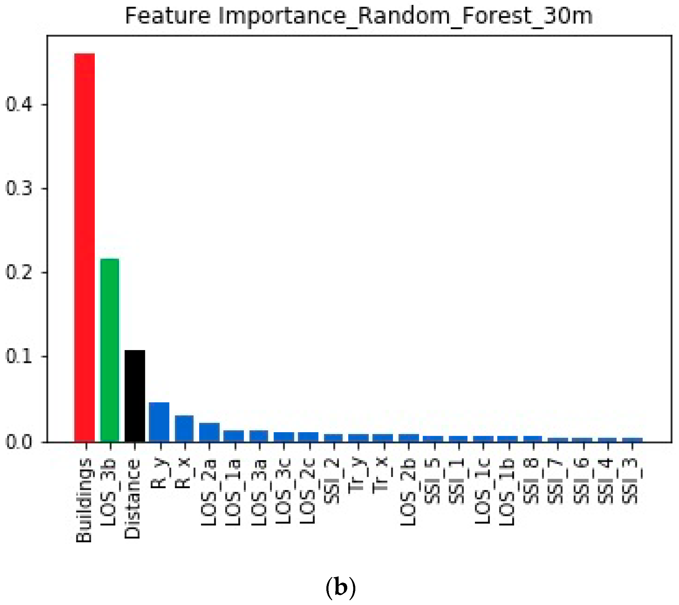
Figure 4 depicts the importance of all of the features. The three most important features (which are denoted via different colors) have the same relative ranking regardless of the machine learning method.
The three most important features are Buildings, LOS_3b, and Distance. Buildings is the top-ranked feature, in accordance with the fact that the mechanism of multiple reflections is expected to be strong at the particular transmitter’s height. It is also worth observing that the importance of LOS_3b (which indicates the presence of the over-rooftop diffraction) is significant, particularly when XGBoost is applied.
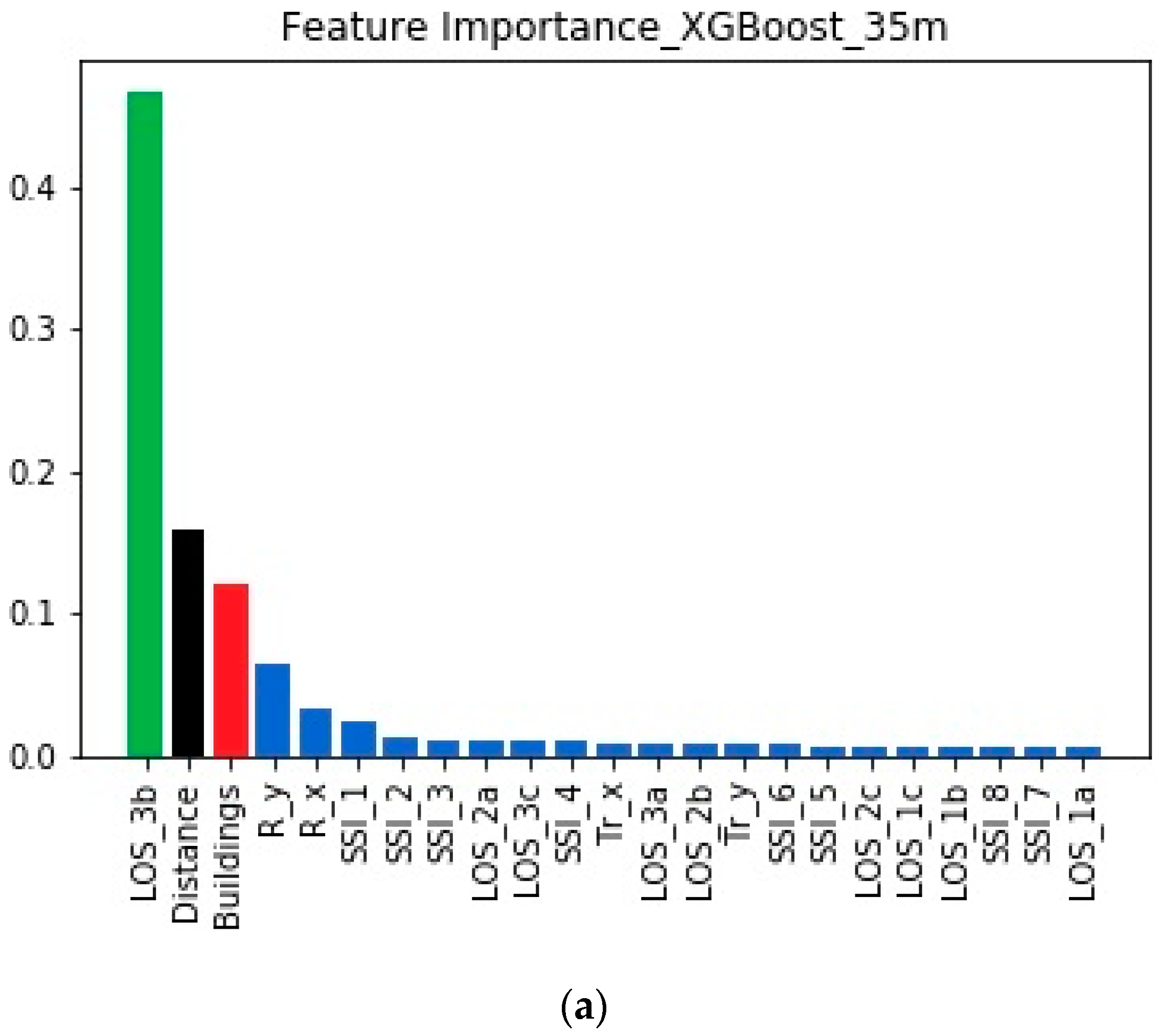
4.3. Feature Importances When the Transmitter is at 35 m
The feature importances for the 35 m case can be found in Figure 5.
According to both models, the same set of three features was found to be the most important for this height. However, the inner ranking between the three features changed: LOS_3b was clearly the most important, indicating that over-rooftop diffraction is the primary propagation mechanism for this height of the transmitter. Moreover, the importance of Buildings fell, since the contribution of multiple reflections decreased.
4.4. Gradual Addition of Features with Reverse Order of Importance
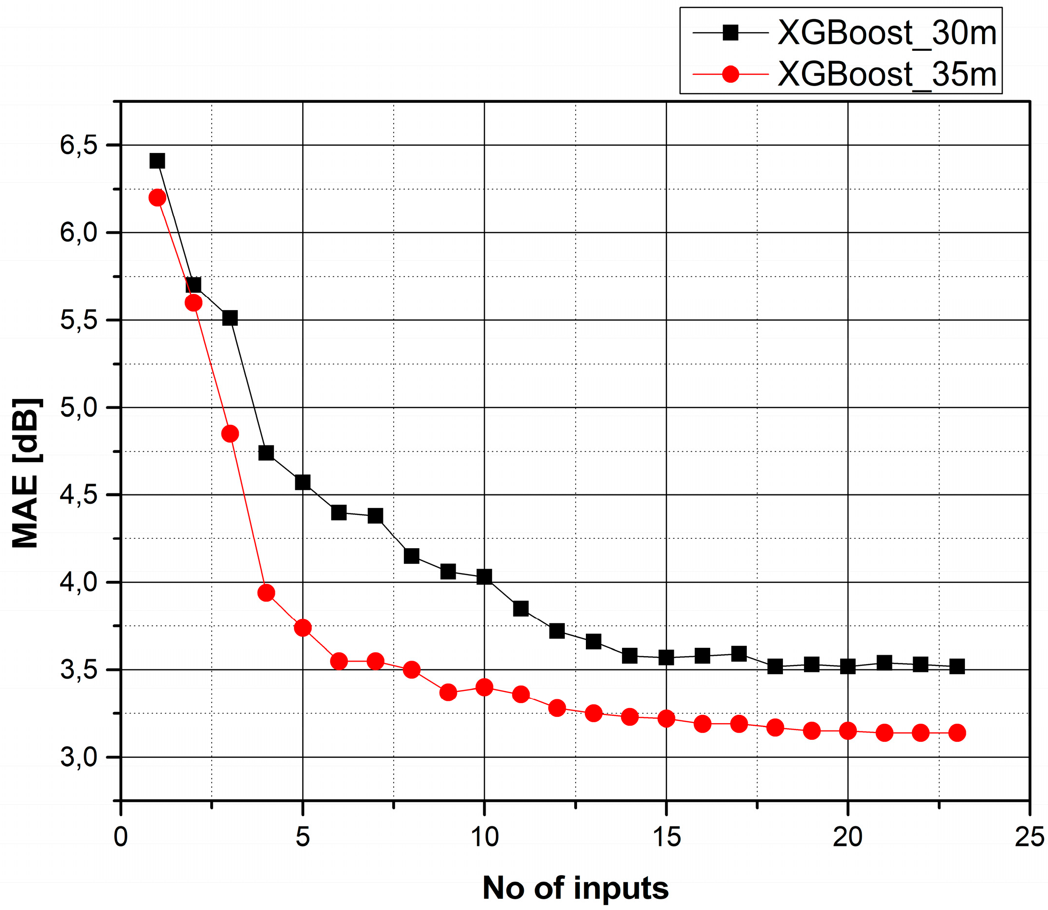
Feature importances can be used to perform feature selection. That is, a subset of the most important features can be selected to construct a simpler machine learning model.
This concept was investigated for both heights using Figure 6. Starting from the most important feature (as calculated from XGBoost) for each height, new features are progressively added according to their importance. After the addition of each new feature, the model’s performance is evaluated.
It is evident that the incorporation of features with the lowest importance does not lead to significant performance improvement.
4.5. Model Reduction
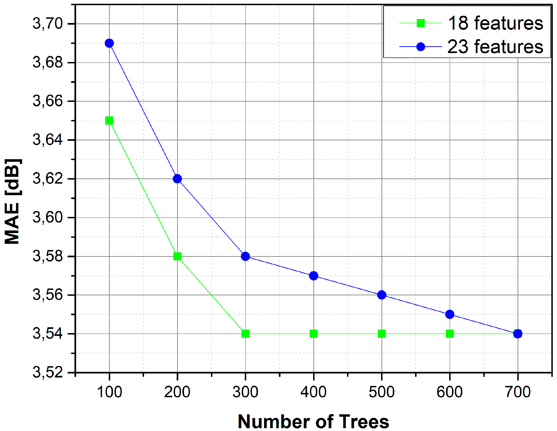
As Figure 6 suggests, the subset of the 18 most important features leads to the same MAE with that obtained when using the full set of 23 features (for the 30 m case). Thus, the application of models with lower complexity can be attempted because fewer features are required. An investigation of the number of trees, the features used, and the MAE value is shown in Figure 7.
It is evident that the full set of features requires more trees to obtain the minimum error. By comparison, the reduced subset produces the same result with lower model complexity. Table 3 presents the training and response times of the models with the lowest MAE values. A computer with an Intel i5-5575R processor and 6 GB of RAM memory was used to train and test the models.
5. Discussion
Feature importance was used as a means to explain the different propagation scenarios that arise when the transmitter is placed at different heights. For both heights, the same set of three features captured more than 75% of the total importance, leaving the remaining 25% (or less) for the remaining 20 features. It is worth mentioning that this behavior is the same according to both machine learning models.
Comparing the inner rankings among the three most important features, it is clear that Buildings outperforms the other features when the transmitter is placed at 30 m. The situation clearly changes when elevating the transmitter to a height of 35 m, in which case LOS_3b becomes the most important feature for this scenario.
It is therefore straightforward to conclude that when the transmitter is placed at 35 m, the mechanism of over-rooftop diffraction has a large influence, because this mechanism is connected with the feature LOS_3b. By comparison, the mechanism of multiple reflections has a stronger influence when the transmitter is placed at 30 m, as concluded through its connection with the feature Buildings.
A closer look at Figure 4; Figure 5 helps explain why the prediction for the 30 m case is worse than that for the 35 m case: for the 35 m case, the dominance of LOS_3b is much clearer than the dominance of Buildings for the 30 m case. That is, over-rooftop diffraction is clearly greater in the 35 m case, whereas the propagation profile of the 30 m case cannot be attributed with the same level of clarity to a single mechanism. This sharper propagation profile makes prediction for the 35 m case easier for the machine learning models, in contrast to the 30 m case, in which the existence of different mechanisms makes the simulation more challenging.
This can also be observed in Figure 6: the error curve drops at a much faster pace in the 35 m case, meaning that a small number of features contains a significant amount of the information needed to model the propagation scenario. However, in the 30 m case the improvement takes place more smoothly, as indicated by the small drops in the prediction error. This is due to the co-existence of different propagation mechanisms for the particular transmitter height.
6. Conclusions and Future Work
Our work highlighted the significance of feature importances, both as a tool to explain radio propagation, and a means to perform feature elimination and reduce model complexity. The emergence of different propagation mechanisms, for two different transmitter heights, was associated with the difference between the values of feature importances. Moreover, model reduction on the basis of the ranked feature importances was performed, leading to substantially faster, although equally accurate, predictions.
The acquisition of more data regarding other transmitter heights, or frequencies, could pave the way to an extension of our work, through the incorporation of the aforementioned parameters as extra features. A single model would then be able to provide results for various propagation scenarios.
Author Contributions
Conceptualization, S.P.S.; methodology, K.S.; software, S.P.S.; writing—original draft preparation, S.P.S. and K.S.; writing—review and editing, S.K.G.; supervision, K.S. and S.K.G. All authors have read and agreed to the published version of the manuscript.
Funding
This research received no external funding.
Conflicts of Interest
The authors declare no conflict of interest.
References
- Sotiroudis, S.P.; Siakavara, K.; Sahalos, J.N. A Neural Network Approach to the Prediction of the Propagation Path-loss for Mobile Communications Systems in Urban Environments. PIERS Online 2007, 3, 1175–1179. [Google Scholar] [CrossRef] [Green Version]
- Faruk, N.; Surajudeen-Bakinde, N.T.; Popoola, S.I.; Olawoyin, L.A.; Atayero, A.A.; Abdulkarim, A.; Abdulkarim, A. ANFIS Model for Path Loss Prediction in the GSM and WCDMA Bands in Urban Area. Elektr. J. Electr. Eng. 2019, 18, 1–10. [Google Scholar] [CrossRef] [Green Version]
- Sotiroudis, S.P.; Goudos, S.K.; Siakavara, K. Deep learning for radio propagation: Using image-driven regression to estimate path loss in urban areas. ICT Express 2020. [Google Scholar] [CrossRef]
- Wen, J.; Zhang, Y.; Yang, G.; He, Z.; Zhang, W. Path Loss Prediction Based on Machine Learning Methods for Aircraft Cabin Environments. IEEE Access 2019, 7, 159251–159261. [Google Scholar] [CrossRef]
- Adeogun, R.O. Calibration of Stochastic Radio Propagation Models Using Machine Learning. IEEE Antennas Wirel. Propag. Lett. 2019, 18, 2538–2542. [Google Scholar] [CrossRef]
- Sotiroudis, S.P.; Goudos, S.K.; Gotsis, K.A.; Siakavara, K.; Sahalos, J.N. Optimal Artificial Neural Network design for propagation path-loss prediction using adaptive evolutionary algorithms. In Proceedings of the 2013 7th European Conference on Antennas and Propagation (EuCAP), Gothenburg, Sweden, 8–12 April 2013; pp. 3795–3799. [Google Scholar]
- Sotiroudis, S.P.; Goudos, S.K.; Gotsis, K.A.; Siakavara, K.; Sahalos, J.N. Application of a Composite Differential Evolution Algorithm in Optimal Neural Network Design for Propagation Path-Loss Prediction in Mobile Communication Systems. IEEE Antennas Wirel. Propag. Lett. 2013, 12, 364–367. [Google Scholar] [CrossRef]
- Zhang, Y.; Wen, J.; Yang, G.; He, Z.; Luo, X. Air-to-Air Path Loss Prediction Based on Machine Learning Methods in Urban Environments. Wirel. Commun. Mob. Comput. 2018, 2018, 1–9. Available online: https://www.hindawi.com/journals/wcmc/2018/8489326/ (accessed on 27 July 2020). [CrossRef]
- Zhang, Y.; Wen, J.; Yang, G.; He, Z.; Wang, J. Path Loss Prediction Based on Machine Learning: Principle, Method, and Data Expansion. Appl. Sci. 2019, 9, 1908. [Google Scholar] [CrossRef] [Green Version]
- Goldsmith, A.; Greenstein, L. A measurement-based model for predicting coverage areas of urban microcells. IEEE J. Sel. Areas Commun. 1993, 11, 1013–1023. [Google Scholar] [CrossRef]
- Saunders, S.R. Antennas and Propagation for Wireless Communication Systems; Wiley: New York, NY, USA, 1999. [Google Scholar]
- Maciel, L.R.; Bertoni, H.L.; Xia, H.N. Unified approach to prediction of propagation over buildings for all ranges of base station antenna height. IEEE Trans. Veh. Technol. 1993, 42, 41–45. [Google Scholar] [CrossRef]
- Goncalves, N.; Correia, L.M. A propagation model for urban microcellular systems at the UHF band. IEEE Trans. Veh. Technol. 2000, 49, 1294–1302. [Google Scholar] [CrossRef]
- Popoola, S.I.; Jefia, A.; Atayero, A.A.; Kingsley, O.; Faruk, N.; Oseni, O.F.; Abolade, R.O. Determination of Neural Network Parameters for Path Loss Prediction in Very High Frequency Wireless Channel. IEEE Access 2019, 7, 150462–150483. [Google Scholar] [CrossRef]
- Sotiroudis, S.P.; Siakavara, K. Mobile radio propagation path loss prediction using Artificial Neural Networks with optimal input information for urban environments. AEU Int. J. Electron. Commun. 2015, 69, 1453–1463. [Google Scholar] [CrossRef]
- Sotiroudis, S.P.; Goudos, S.K.; Siakavara, K. Neural Networks and Random Forests: A Comparison Regarding Prediction of Propagation Path Loss for NB-IoT Networks. In Proceedings of the 2019 8th International Conference on Modern Circuits and Systems Technologies (MOCAST), Thessaloniki, Greece, 13–15 May 2019; pp. 1–4. [Google Scholar] [CrossRef]
- Sotiroudis, S.P.; Goudos, S.K.; Gotsis, K.A.; Siakavara, K.; Sahalos, J.N. Modeling by optimal Artificial Neural Networks the prediction of propagation path loss in urban environments. In Proceedings of the 2013 IEEE-APS Topical Conference on Antennas and Propagation in Wireless Communications (APWC), Torino, Italy, 9–13 September 2013; pp. 599–602. [Google Scholar] [CrossRef]
- Piacentini, M.; Rinaldi, F. Path loss prediction in urban environment using learning machines and dimensionality reduction techniques. Comput. Manag. Sci. 2010, 8, 371–385. [Google Scholar] [CrossRef] [Green Version]
- OpenStreetMap Contributors S. Planet Dump. Available online: https://planet.osm.org (accessed on 27 July 2020).
- Chen, T.; Guestrin, C. XGBoost: A Scalable Tree Boosting System. In Proceedings of the 22nd ACM SIGKDD International Conference on Knowledge Discovery and Data Mining, San Francisco, CA, USA, 13–17 August 2016; pp. 785–794. [Google Scholar] [CrossRef] [Green Version]
- Breiman, L. Random Forests. Mach. Learn. 2001, 45, 5–32. [Google Scholar] [CrossRef] [Green Version]
- Hastie, T. The Elements of Statistical Learning: Data Mining, Inference, and Prediction; Springer: New York, NY, USA, 2009. [Google Scholar]
- Kuhn, M.; Johnson, K. Applied Predictive Modeling; Springer: New York, NY, USA, 2013. [Google Scholar]
- EDX Wireless. EDX Wireless Microcell/Indoor Module Reference Manual, Version 7©; EDX Wireless: Eugene, OR, USA, 1996–2011. [Google Scholar]
Figure 1.
The first 10 features [18].
Figure 1.
The first 10 features [18].

Figure 2.
Extraction of features 11 to 18.

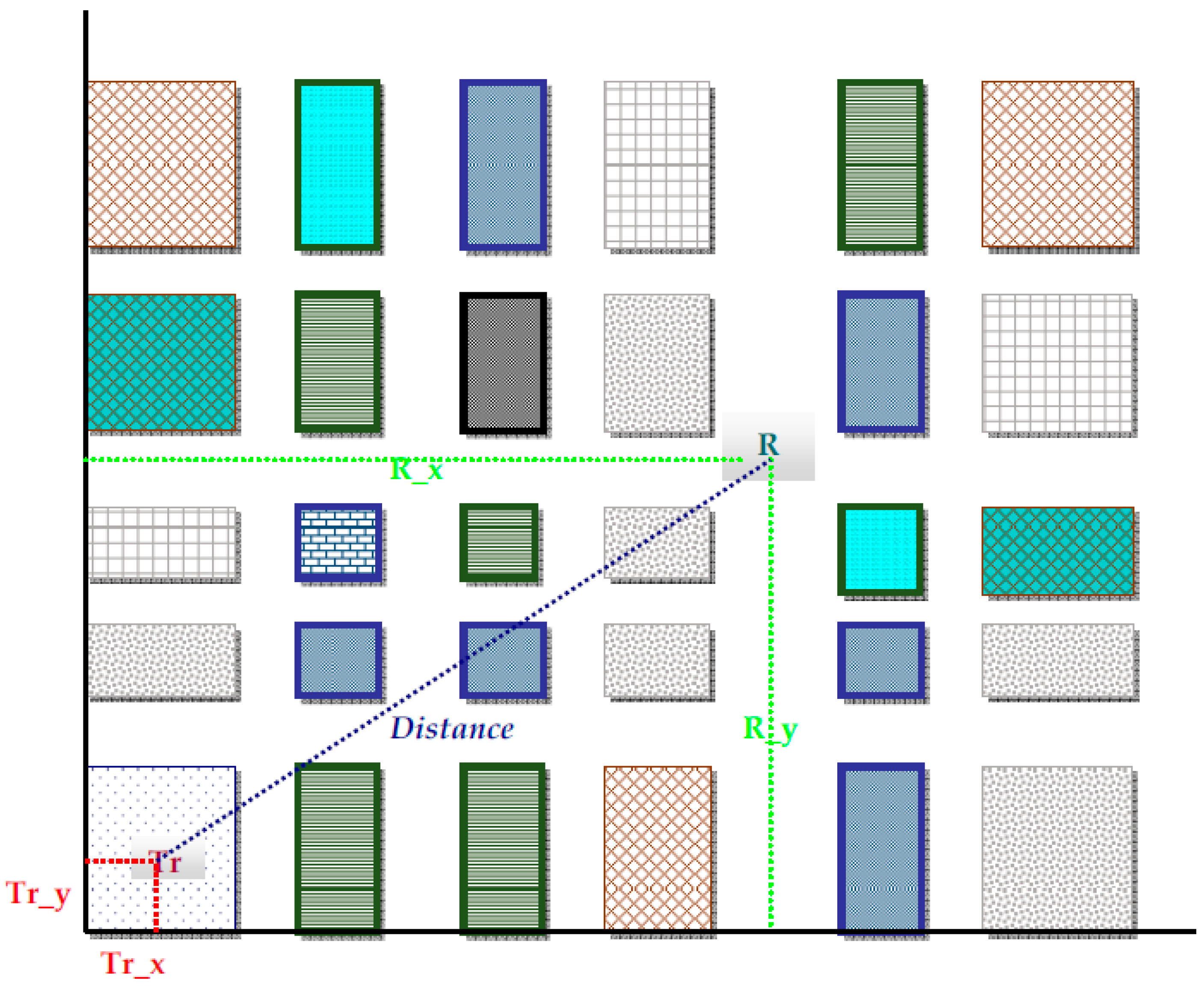
Figure 3.
Features 19 to 23 refer only to the positions of the transmitter and the receiver, and the distance between them. They do not depend on the built-up profile of the area in question. Table 1 summarizes and describes all features.
Figure 3.
Features 19 to 23 refer only to the positions of the transmitter and the receiver, and the distance between them. They do not depend on the built-up profile of the area in question. Table 1 summarizes and describes all features.

Figure 4.
Feature importances, as estimated when the transmitter is placed at 30 m, via two machine learning models: (a) XGBoost; (b) Random Forest. The feature called Buildings is ranked as the most important.
Figure 4.
Feature importances, as estimated when the transmitter is placed at 30 m, via two machine learning models: (a) XGBoost; (b) Random Forest. The feature called Buildings is ranked as the most important.


Figure 5.
Feature importances, as estimated when the transmitter is placed at 35 m, via two machine learning models: (a) XGBoost; (b) Random Forest. The feature called LOS_3b is ranked as the most important.
Figure 5.
Feature importances, as estimated when the transmitter is placed at 35 m, via two machine learning models: (a) XGBoost; (b) Random Forest. The feature called LOS_3b is ranked as the most important.


Figure 6.
Gradual addition of features with reverse order of importance. The improvement is negligible as features of low importance are added.
Figure 6.
Gradual addition of features with reverse order of importance. The improvement is negligible as features of low importance are added.

Figure 7.
The XGBoost model obtains the minimum MAE value with a smaller number of trees for an optimum input subset of 18 features (for the 30 m case).
Figure 7.
The XGBoost model obtains the minimum MAE value with a smaller number of trees for an optimum input subset of 18 features (for the 30 m case).


Table 1.
The 23 features used.
| Number | Name | Description |
|---|---|---|
| 1 | LOS_1a | The distance (h1) of the top of the tallest building of the first segment, from the point at which the building intersects the LOS ray, between Tr and R |
| 2 | LOS_1b | The distance d1 of the tallest building of the first segment from the transmitter |
| 3 | LOS_1c | The length, l1, of the tallest building of the first segment |
| 4 | LOS_2a | The distance (h2) of the top of the tallest building of the second segment, from the point at which the building intersects the LOS ray, between Tr and R |
| 5 | LOS_2b | The distance d2 of the tallest building of the second segment from the transmitter |
| 6 | LOS_2c | The length, l2, of the tallest building of the second segment |
| 7 | LOS_3a | The distance (h3) of the top of the tallest building of the third segment, from the point at which the building intersects the LOS ray, between Tr and R |
| 8 | LOS_3b | The distance d3 of the tallest building of the first segment from the transmitter |
| 9 | LOS_3c | The length, l3, of the tallest building of the third segment |
| 10 | Buildings: | The total number of the buildings which interrupt the LOS path. |
| 11 | SSI_1 | The height of the building (or the existence of a street) 10m right from the receiver |
| 12 | SSI_2 | The height of the building (or the existence of a street) 10 m left from the receiver |
| 13 | SSI_3 | The height of the building (or the existence of a street) 10 m above the receiver |
| 14 | SSI_4 | The height of the building (or the existence of a street) 10 m below the receiver |
| 15 | SSI_5 | The height of the building (or the existence of a street) 10 m left and above the receiver |
| 16 | SSI_6 | The height of the building (or the existence of a street) 10 m left and below the receiver |
| 17 | SSI_7 | The height of the building (or the existence of a street) 10 m right and above the receiver |
| 18 | SSI_8 | The height of the building (or the existence of a street) 10 m right and below the receiver |
| 19 | Tr_x | X_coordinate of the transmitter |
| 20 | Tr_y | Y_coordinate of the transmitter |
| 21 | R_x | X_coordinate of the receiver |
| 22 | R_y | Y_coordinate of the receiver |
| 23 | Distance | The distance between transmitter and receiver in the xy plane |
Table 2.
Error metrics according to both methods for two transmitter heights.
| Transmitter Height (m) | XGBoost | Random Forest | ||
|---|---|---|---|---|
| MAE (dB) | R2 | MAE (dB) | R2 | |
| 30 | 3.54 | 0.89 | 3.97 | 0.87 |
| 35 | 3.17 | 0.91 | 3.35 | 0.90 |
Table 3.
Time comparison of XGBoost models with the same MAE, for the 30 m case. (Data in bold font indicates the smaller values.)
Table 3.
Time comparison of XGBoost models with the same MAE, for the 30 m case. (Data in bold font indicates the smaller values.)
| Model No | MAE (dB) | Trees | Features | Training Time (s) | Response Time (ms) |
|---|---|---|---|---|---|
| 1 | 3.54 | 700 | 23 | 68.34 | 382.51 |
| 2 | 3.54 | 700 | 18 | 58.46 | 354.79 |
| 3 | 3.54 | 300 | 18 | 32.02 | 147.88 |
© 2020 by the authors. Licensee MDPI, Basel, Switzerland. This article is an open access article distributed under the terms and conditions of the Creative Commons Attribution (CC BY) license (http://creativecommons.org/licenses/by/4.0/).
Share and Cite
MDPI and ACS Style
Sotiroudis, S.P.; Goudos, S.K.; Siakavara, K. Feature Importances: A Tool to Explain Radio Propagation and Reduce Model Complexity. Telecom 2020, 1, 114-125. https://0-doi-org.brum.beds.ac.uk/10.3390/telecom1020009
AMA Style
Sotiroudis SP, Goudos SK, Siakavara K. Feature Importances: A Tool to Explain Radio Propagation and Reduce Model Complexity. Telecom. 2020; 1(2):114-125. https://0-doi-org.brum.beds.ac.uk/10.3390/telecom1020009
Chicago/Turabian StyleSotiroudis, Sotirios P., Sotirios K. Goudos, and Katherine Siakavara. 2020. "Feature Importances: A Tool to Explain Radio Propagation and Reduce Model Complexity" Telecom 1, no. 2: 114-125. https://0-doi-org.brum.beds.ac.uk/10.3390/telecom1020009