
Stock Market Prediction Using Microblogging Sentiment Analysis and Machine Learning


School of Science and Technology, International Hellenic University, 57001 Thessaloniki, Greece
*
Author to whom correspondence should be addressed.
Telecom 2022, 3(2), 358-378; https://0-doi-org.brum.beds.ac.uk/10.3390/telecom3020019
Submission received: 29 March 2022
/
Revised: 23 May 2022
/
Accepted: 23 May 2022
/
Published: 27 May 2022
(This article belongs to the Special Issue Selected Papers from SEEDA-CECNSM 2021)
Abstract
:The use of Machine Learning (ML) and Sentiment Analysis (SA) on data from microblogging sites has become a popular method for stock market prediction. In this work, we developed a model for predicting stock movement utilizing SA on Twitter and StockTwits data. Stock movement and sentiment data were used to evaluate this approach and validate it on Microsoft stock. We gathered tweets from Twitter and StockTwits, as well as financial data from Finance Yahoo. SA was applied to tweets, and seven ML classification models were implemented: K-Nearest Neighbors (KNN), Support Vector Machine (SVM), Logistic Regression (LR), Naïve Bayes (NB), Decision Tree (DT), Random Forest (RF) and Multilayer Perceptron (MLP). The main novelty of this work is that it integrates multiple SA and ML methods, emphasizing the retrieval of extra features from social media (i.e., public sentiment), for improving stock prediction accuracy. The best results were obtained when tweets were analyzed using Valence Aware Dictionary and sEntiment Reasoner (VADER) and SVM. The top F-score was 76.3%, while the top Area Under Curve (AUC) value was 67%.
1. Introduction
Stock exchanges have become an important element of the economy, as they promote financial and capital gain [1]. A stock market is a network of economic transactions in which shares are bought and sold. The ownership claims on enterprises are mirrored in the equity or market share. This might include shares originating from the public stock market or through individual trading, such as shares of private enterprises traded to investors. Transactions in stock markets are described as the process of shifting money from small individual investors to large trading investors, such as banks and corporations. However, stock market investment is regarded as a high-risk practice due to the occurrence of erratic behavior [2].
If performed correctly, Stock Market Prediction (SMP) may be quite beneficial to investors. The efficient prediction of stock prices may provide shareholders with useful assistance in making suitable decisions about whether to purchase or sell shares. The act of attempting to anticipate the future value of a stock is defined as SMP. Several approaches for predicting stock prices have been presented over the years. In general, they are divided into four groups. The first is basic analysis, which is based on publicly available financial information. The second kind is technical analysis, which involves making recommendations based on previous data and pricing. The third includes the use of Machine Learning (ML) and Data Mining (DM) massive volumes of data gathered from various sources. The last is Sentiment Analysis (SA), which makes predictions based on previously published news, articles, or blogs [3,4]. The mixture of the last two groups is more recent than the previous two, and research suggests that they may exert more influence on whether to buy or sell stocks [5].
This paper provides a strategy for predicting stock movements using ML methods and SA. SA is accomplished by the use of publicly accessible information from microblogging networks such as Twitter and StockTwits, which give crucial insights into people’s emotions. According to a widespread hypothesis, when public perception towards a firm is good, stock prices tend to rise, and the other way round [6]. However, when additional economic aspects are included, this idea is not always validated.
Microsoft stock is employed as an example, and we evaluate price fluctuations based on financial and sentiment data. From 16 July 2020 to 31 October 2020, 90,000 tweets from Twitter and 7440 tweets from StockTwits were gathered. During the same time-period, financial data were also collected from Finance Yahoo. TextBlob and Valence Aware Dictionary and sEntiment Reasoner (VADER) were used to perform SA on these tweets. Furthermore, seven ML models were incorporated, including K-nearest neighbors (KNN), Support Vector Machine (SVM), Logistic Regression (LR), Nave Bayes (NB), Decision Tree (DT), Random Forest (RF), and Multilayer Perceptron (MLP), as well as two performance evaluation metrics, F-score and Area Under Curve (AUC). When utilizing data from Twitter with VADER as a sentiment analyzer, the results show that SVM has the greatest F-score of 76.3% and an AUC value of 67%.
The rest of the paper is organized as follows. Section 2 gives context and an assessment of the state of the art. Our methodology is described in depth in Section 3, and the assessment of outcomes is discussed in Section 4. The study concludes with Section 5, which discusses accomplishments, limitations/challenges, and future work.
2. Background
This section reviews state-of-the-art efforts to identify stock-market movements using SA on microblogging data, as well as the classification methods and performance assessment measures utilized in this work.
2.1. Sentiment Analysis Applications
SA on Social Media (SM) data from various SM platforms and types [7] has played a vital role in prediction in a variety of sectors (e.g., healthcare, financial etc.). It is the process of determining whether ideas conveyed in texts are positive or negative to the topic of discussion. Some of its advantages include analytics [8], which may help in the advancement of marketing plans, enhancement of customer service, growth of sales income, identification of unwanted rumors for risk mitigation, and so on [9]. Here, we will demonstrate several such prominent studies, with an emphasis on SMP utilizing data from Twitter or StockTwits.
SVM and NB algorithms were utilized to analyze public sentiment and its connection to stock market prices for the 16 most popular IT firms, such as Microsoft, Amazon, Apple, Blackberry, and others. They achieved 80.6% accuracy with NB and 79.3% accuracy with SVM on predicting sentiment utilizing seven-fold cross-validation. Furthermore, in the presence of noise in data, the prediction error for all of the tech businesses was determined to be less than 10%. Overall, the average prediction error in all cases was 1.67%, indicating an excellent performance [10].
The association between a company’s stock-market movements and the emotion of tweet messages was investigated using SA and ML. Tweets, as well as stock opening and closing prices, were retrieved for Microsoft from the Yahoo Finance website between 31 August 2015 and 25 August 2016. Models were created with 69.01% and 71.82% accuracy using the LR and LibSVM methods, respectively. Accuracy with a big dataset was greater, and it was identified that there was a connection between stock-market movements and twitter public sentiment [11].
The relationship between tweets and Dow Jones Industrial Average (DJIA) values was investigated by collecting Twitter data between June and December of 2009. A total of 476 million tweets were acquired from almost 17 million individuals. The timestamp and tweet text were chosen as features. The DJIA values were obtained from Yahoo Finance spanning the months June to December of 2009. The open, close, high, and low values for a specific day were chosen as features. The stock values were preprocessed by substituting missing data and calculating the average for DJIA on a particular day and the following one. In addition, instances when the data were inconsistent and making predictions was more challenging were omitted. Tweets were divided into four categories: calm, happy, alert, and kind. They used four ML algorithms to train and test the model after examining the causality relationship between both the emotions of the previous three days and the stock prices of the current day. These algorithms included Linear/Logistic Regression, SVM and Self Organizing Fuzzy (SOF) Neural Networks (NN). Six combinations were tested, using the emotion scores from the previous three days to rule out the possibility of other emotional factors being dependent on DJIA. With 75.56% accuracy, SOF NN achieved the best performance combining happy, calm, and DJIA. It was also discovered that adding any additional emotional type reduced accuracy [12].
The relationship between Saudi tweets and the Saudi stock index was also investigated. Mubasher’s API, which is a stock analysis software, was utilized to obtain tweets. A total of 3335 tweets were retrieved for 53 days ranging from 17 March 2015 to 10 May 2015, as well as the TASI index’s closing prices. SA was carried out, utilizing ML techniques such as NB, SVM and KNN. SVM accuracy was 96.6%, while KNN accuracy was 96.45%. The results showed that as negative sentiment increased, positive sentiment and TASI index decreased, indicating a coherent correlation between sentiment and TASI index [13].
An Apple’s stock forecast was performed, exploiting a mix of StockTwits and financial data retrieved between 2010 and 2017. SVM was used to estimate public opinion and whether or not a person would purchase or sell a stock. Three attributes were chosen for the model: date, stock price choices, and sentiment. The accuracy of the training and test models was 75.22% and 76.68%, respectively. The authors claim that the findings may be improved by expanding the volume of the data collection [14].
The relationship between StockTwits emotion and stock price fluctuations was investigated for five businesses, including Microsoft, Apple, General Electric, Target, and Amazon. Stock market and StockTwits data were gathered from 1 January 2019 to 30 September 2019. SA was conducted by utilizing three classifiers (LR, NB and SVM) and five featurization algorithms (bigram, LSA, trigram, bag of words and TF-IDF). This implementation was created to anticipate stock price changes for a day using both financial data and collected feelings from the preceding five days. According to the performance evaluation, accuracy varied from 62.3% to 65.6%, with Apple and Amazon exhibiting the greatest results [15].
Another study focused on the high stock market capitalization and a distinctive SM ecosystem to investigate the link between stock price movements and SM sentiment in China [16]. Collected data varied in terms of activity, post length, and association with stock market performance. Stock market chatroom users tended to write more but shorter blogs. Trading hours and volume were far more closely linked to activity. Multiple ML models were incorporated to identify post sentiment in chatrooms, and produced results comparable to the current state of the art. Because of the substantial connection and Granger causality between chatroom post sentiment and stock price movement, post sentiment may be utilized to enhance stock price prediction over only analyzing historical trade data. Furthermore, a trading strategy was designed based on the prediction of trading indicators. This buy-and-hold strategy was tested for seven months and yielded a 19.54% total return, versus a loss of −25.26%.
Authors in [17] consider three distinct equities’ closing prices and daily returns to examine how SM data may predict Tehran Stock Exchange (TSE) factors. Three months of StockTwits were gathered. A lexicon-based and learning-based strategy was proposed to extract data from online discussions. Additionally, a custom sentiment lexicon was created, since existing Persian lexicons are not suitable for SA. Novel predictor models utilizing multi-regression analysis were proposed after creating and computing daily sentiment indices based on comments. The number of comments and the users’ trustworthiness were also considered in the analysis. Findings show that the predictability of TSE equities varies by their features. For estimating the daily return, it is shown that both comment volume and mood may be beneficial, and the three stocks’ trust coefficients behave differently.
Stock price prediction is a topic with both potential and obstacles. There are numerous recent stock price prediction systems, yet their accuracy is still far from sufficient. The authors of [18] propose S_I_LSTM, a stock price prediction approach that includes numerous data sources as well as investor sentiment. First, data from different Internet sources are preprocessed. Non-traditional data sources such as stock postings and financial news are also included. Then, for non-traditional data, a Convolutional Neural Network (CNN) SA approach is applied to generate the investor sentiment index. As a last step, a Long Short-Term Memory (LSTM) network is utilized to anticipate the Shanghai A-share market. It incorporates sentiment indexes, technical indicators, and historical transaction data. With a Mean Absolute Error (MAE) value of 2.38, this approach outperforms some existing methods when compared to actual datasets from five listed businesses.
Another research study suggests a SMP system based on financial microblog sentiment from Sina Weibo [19]. SA was performed on microblogs to anticipate stock market movements using historical data from the Shanghai Composite Index (SH000001). The system contained three modules: Microblog Filter (MF), Sentiment Analysis (SA), and Stock Prediction (SP). Financial microblog data were obtained by incorporating Latent Dirichlet Allocation (LDA). The SA module first builds a financial vocabulary, then obtains sentiment from the MF module. For predicting SH000001 price movements, the SP module presents a user-group model that adjusts the relevance of various people and blends it with previous stock data. This approach was proven to be successful, since it was tested on 6.1 million microblogs.
SA on microblogs has recently become a prominent business analytics technique investigating how this sentiment can affect SMP. In [20], vector autoregression was performed on a data collection of four years. The dataset contained 18 million microblog messages at a daily and hourly frequency. The findings revealed that microblog sentiment affects stock returns in a statistically and economically meaningful way. Market fluctuation influenced microblog sentiment and stock returns affected negative sentiment more than positive sentiment.
Another study presented a microblogging data model that estimates stock market returns, volatility, and trade volume [21]. Indicators from microblogs (a large Twitter dataset) and survey indices (AAII and II, USMC and Sentix) were used to aggregate these indicators in daily resolution. A Kalman Filter (KF) was used to merge microblog and survey sources. Findings showed that Twitter sentiment and tweeting volume were useful for projecting S&P 500 returns. Additionally, Twitter and KF sentiment indicators helped forecast survey sentiment indicators. Thus, it is concluded that microblogging data may be used to anticipate stock market activity and provide a viable alternative to traditional survey solutions.
Time-series analysis is a prominent tool for predicting stock prices. However, relying solely on stock index series results in poor forecasting performance. As a supplement, SA on online textual data of the stock market may provide a lot of relevant information, which can act as an extra indicator. A novel technique is proposed for integrating such indicators and stock index time-series [22]. A text processing approach was suggested to produce a weighted sentiment time-series. The data were crawled from financial micro-blogs from prominent Chinese websites. Each microblog was segmented and preprocessed, and the sentiment values were determined on a daily basis. The proposed time-series model with weighted sentiment series was validated by predicting the future value of the Shanghai Composite Index (SSECI).
The authors of [23] investigated a possible association between the Chinese stock market and Chinese microblogs. At first, C-POMS (Chinese Profile of Mood States) was proposed for SA on microblog data. Then, the Granger causality test validated the existence of association between C-POMS and stock prices. Utilizing different prediction models for SMP showed that Support Vector Machine (SVM) outperforms Probabilistic Neural Networks (PNN) in terms of accuracy. Adding a dimension of C-POMS to the input data improved accuracy to 66.66%. Utilizing two dimensions to the input data resulted in 71.42% accuracy, which is nearly 20% greater than just using historical data.
2.2. Classification Algorithms
Classification algorithms are predictive computations that recognize, comprehend, and categorize data [24,25]. A list of such methods utilized in this work is compiled here.
K-nearest Neighbors (KNN) is a lazy and non-parametric algorithm. It computes the distance employing the most popular distance function, the Euclidean distance d, which determines the difference or similarity (or else the shortest distance) between two instances/points and , according to (1).
For a particular value of K, the method will determine the K-Nearest Neighbors of the data point and then assign the class to the data point based on the class with the most data points among the K-Neighbors [26]. Following the calculation of the distance, the input x is allocated to the class with the highest probability according to (2).
Support Vector Machine (SVM) is a classification method that solves binary problems by searching for an optimal hyperplane in high-dimensional space, isolating the points with the greatest margin. If two categories of points are differentiated, then there is a hyperplane that splits them. The purpose of this classification is to calculate a decent separating hyperplane between two outcomes. This is achieved by locating the hyperplane that optimizes the margin in between categories or classes [27]. In more detail, given training vectors , i = 1, …, n, in two classes, and a vector , the main goal is to find and such that the prediction given by is correct for most of the samples. The SVM solves the problem (3):
Therefore, the aim is to minimize , while applying a penalty when a sample is not correctly classified. Preferably, the value would be ≥1 for all of the samples indicating a perfect prediction. Nonetheless, problems are not always perfectly separable with a hyperplane allowing some samples to be at a distance from their ideal margin boundaries.
Logistic Regression (LR) is classification technique estimating the likelihood that an observation belongs to one of two classes (1 or 0). LR employs a complicated function (sigmoid), which transfers predicted values to their corresponding distributions of likelihoods. The logistic function is a sigmoid function given by (4) and pushes the values from (−n, n) to (0, 1) [28].
Naive Bayes (NB) is a classification technique that may be used for binary and multi-class classification. NB techniques are a type of supervised learning algorithms that use Bayes’ theorem with the ‘naive’ assumption of conditional independence between every pair of features given a class variable y and a dependent feature vector from to , as stated in (5). When compared to numerical variables, NB performs well with categorical input data. It is helpful for anticipating data and creating predictions based on past findings [29].
Decision Tree (DT) is a classification method that uses decision rules to predict the class of the target variable. For the purpose of creating a tree, the ‘divide and conquer’ strategy can be used. The parameter utilized for the root node is chosen because it has a high p-value, and then the tree is partitioned into sub trees. The sub trees are further divided, employing the same technique until they get to the leaf node. Decision rules can be derived only after the tree has been created [30]. In more detail, given some training vectors , i = 1, …, l and a label vector , a decision tree recursively partitions the feature space in a way that the samples with the same labels or similar target values belong to the same group.
Let the data at node m be represented by with samples. For each candidate split that consists of a feature j and threshold , partition the data into and subsets (6):
The quality of a candidate split of node m is then calculated, utilizing an impurity function for classification problems (7).
Then, select the respected parameters that minimize the impurity (8):
Finally, recurse for subsets and until the point that the maximum depth allowed, or .
Random Forest (RF) is an ensemble learning approach comprising numerous arbitrary generated DTs. Random Forest seeks the greatest feature from an arbitrary feature subset, with the goal of using it as a criterion for dividing the nodes. RF solves the problem of over-fitting and delivers higher accuracy predictions than regular DTs [31].
The Multilayer Perceptron (MLP) is a deep artificial NN and supervised learning approach. MLP is made up of numerous layers of input nodes connected by a directed graph that connects the input and output layers. The signal is fed into the input layer, and the prediction is made by the output layer. The purpose is to estimate the best relationship between the input and output layers [32]. Given a set of training examples where and , a one-hidden layer one-hidden neuron MLP learns the function where and are model parameters. represent the weights of the input layer and hidden layer, respectively, while show the bias added to the hidden layer and the output layer, respectively. is the activation function, set by default as the hyperbolic tan according to (9).
For binary classification, passes through the logistic function to retrieve output values between zero and one. A threshold is set to 0.5, assigning samples of outputs larger or equal 0.5 to the positive class, and the remainder to the negative class.
The MLP loss function for classification is the Average Cross-Entropy, which in binary case is calculated according to (10).
In a gradient descent, the gradient of the loss concerning the weights is calculated and subtracted from W according to (11), where k is the iteration step and stands as the learning rate with a greater value from zero. The algorithm terminates when the maximum number of iterations is reached, or when the gain in loss is less than a particular, very small threshold.
2.3. Performance Evaluation Metrics
To examine the behaviors of classification algorithms, certain evaluation measures were utilized. In this work, we incorporate F-score and AUC to assess the algorithms, but we also provide the short definitions of Precision, Recall, Sensitivity, Specificity, and Receiver Operator Characteristic (ROC) curve, since they are essential for the computation and definition of F-score and AUC [33].
Precision is defined as the proportion of true positives to all anticipated positive instances (12). Recall is the proportion of true positives to all positive cases (13).
The harmonic mean of accuracy and recall is computed using the F-score. This score considers both false positives and false negatives (14).
ROC curve is a binary classification problem assessment measure. It is a probability curve that shows the True Positive Rate (Sensitivity) (15) against the False Positive Rate (1-Specificity) (16) at various threshold levels, separating the ‘signal’ from ‘noise.’
AUC is a measure that discriminates between classes and is used to summarize the ROC curve. The greater the AUC, the stronger the model’s ability to differentiate between positive and negative classifications. When AUC = 1, the classifier successfully distinguishes between all positive and negative class points. On the other hand, if the AUC is 0, the classifier classifies all positives as negatives and all negatives as positives.
3. Research Design
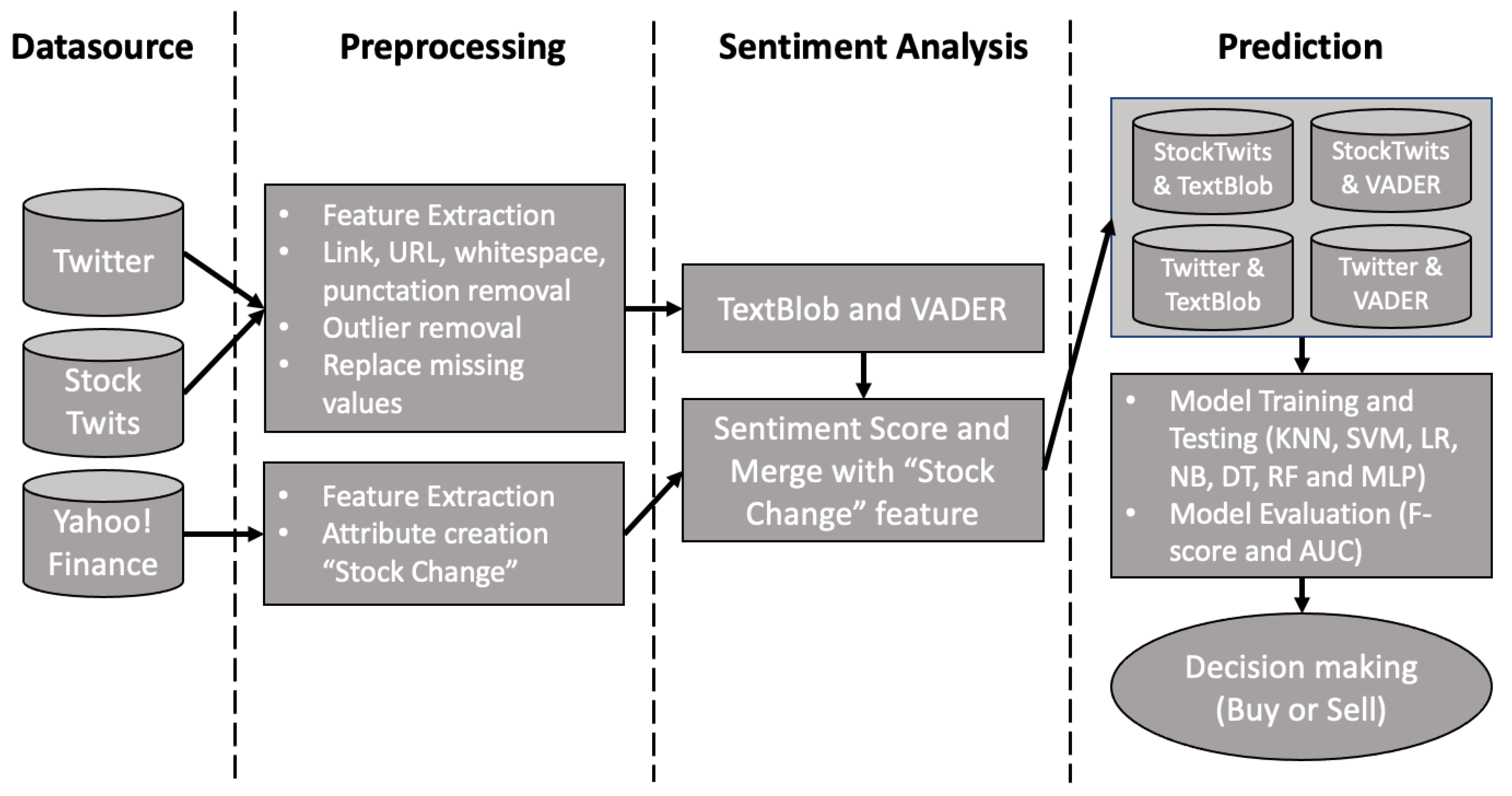
In this study, we introduce a methodology for predicting stock movement utilizing SA on Twitter and StockTwits data. Exploiting APIs, we first extract tweets from Twitter and stock tweets from StockTwits. We then use methods such as TextBlob and VADER to apply SA to text. VADER is an SM data lexicon and a rule-based SA tool. It not only returns positive, neutral, or negative numbers, but also evaluates how positive or negative a sentiment is [34]. TextBlob, on the other hand, is a SA library that returns a sentiment rating for each tweet [35].
Following that, financial information from Yahoo Finance was pulled. The stock price movements, the stock change variable, are then combined with the sentiment scores, and the SMP model is built using seven classifiers. To evaluate the suggested model, we divided the data into training and test sets. We appoint 80% for training the model and 20% for testing in accordance with the Pareto Principle [36]. The proposed approach for anticipating stock movement is displayed in Figure 1.
3.1. Data Collection
For estimating Microsoft’s stock price, we gathered financial data from the Yahoo Finance website and SM data, including Twitter data, as well as stock Twitter data from StockTwits, for the timeframe from 16 July 2020 to 31 October 2020 summing up to 108 days. The SMP will be divided into two sections. The first involves the utilization of Twitter data and financial data, while the second involves the utilization of StockTwits data and financial data.
3.1.1. Twitter Data
To connect to Twitter’s API, a developer account was generated. We gathered and sorted Tweets in English using keywords such as #Microsoft, #MSFT, and #Microsoft365. During the timeframe from 16 July 2020 to 31 October 2020, a total of 90,000 tweets were crawled from Twitter.
We retrieved the user ID, keyword, user account, tweet text, and date of creation, as shown in Table 1.
3.1.2. StockTwits Data
The search API was used to retrieve stock tweets based on language, time, and firm ticker. After importing the requests library, the server responds with a JSON object containing tweets. A firm ticker, such as $MSFT, was used to extract tweets. For the time frame from 16 July 2020 to 31 October 2020, 7440 tweets were retrieved from StockTwits.
The collected tweets were stored as it is shown in Table 2 keeping just the necessary attributes (ID, text and date).
3.1.3. Financial Data
Microsoft’s historical records were gathered from Yahoo! Finance, which contains massive volumes of worldwide market data, current news, stock quotes, and portfolio materials [37].
The features gathered were closing and opening price, low and high price, volume, and adjusted price (Table 3). Between 16 July 2020 and 31 October 2020, 77 dates of such information were obtained from Yahoo! Finance.
3.2. Data Preprocessing
Symbol removal, outlier removal, replacing missing values, and feature selection are among the data preparation stages that were conducted.
3.2.1. Symbol Removal
We eliminated some symbols before conducting SA, such as @, $, URLs, additional spaces, and punctuation marks, since they provide no value to SA.
3.2.2. Outlier Removal
After collecting the data, we standardized the sentiment score around the mean to be equal to zero with a standard deviation of one. Importing the class ‘StandardScaler’ and its methods from the ‘sklearn.preprocessing’ module [38], we enforced data consistency so that each data point has the same range and variability. Then, outliers in the sentiment dataset were deleted. Outliers endanger the model’s validity, since they make up a significant portion of the primary datasets, as seen in Table 4.
Therefore, to reduce bias, significant positive or negative rates were excluded. We utilized the 10% for small rates as flooring and the 90% for large rates as topping thresholds, respectively.
3.2.3. Replacing Missing Values
Acquiring tweets for all days was impossible due to Twitter’s seven-day restriction for retrieving tweets. As a result, the mean value was used to replace the missing sentiments. Furthermore, stock data were absent on weekends or when the stock market was down. Therefore, to retrieve relevant values, we employed a function that linearly interpolates between known data to generate unknown values. Linear interpolation is a method for approximating unknown values that seem to be among the known ones [39].
3.2.4. Feature Selection
We employed low and high price, volume, and adjusted price as input qualities for this task, and we also added two more features. These were the mean sentiment score for each day, which is one of the model’s inputs, and the stock change behavior, which is the goal variable. We determined the average of the sentiment rating for each day, since we obtained several sentiment ratings for one day. Thus, we included a new variable called ‘Stock Change’ to determine if the stock price rises or falls. The closing price was deducted from the open price and divided by the open price to arrive at this conclusion, as shown in (17).
In case the outcome of the stock change is larger than zero, the stock movement is positive and the stock price falls, allowing the buyer to purchase Microsoft stocks. This outcome is denoted by the number 1. Otherwise, if the outcome of the stock movement is negative, the stock price rises and the investor can sell the shares to benefit. This outcome is denoted by the symbol −1.
The distribution of the close and open prices over time is depicted in Figure 2. The red line denotes the open price, while the green line denotes the close price. The open price is extremely similar to the closing price, with only minor differences. When comparing to various time frames of the overall period of stock price movements, it is worth noting that high open and close prices were observed during the end of August and beginning of September.
Lastly, we combined the Twitter with stock data, as well as the StockTwits with stock data. We generated four scenarios as a consequence of using Twitter/StockTwits and stock data with TextBlob and VADER. For each of the four scenarios, we built a dataset with two columns containing sentiment values ranging from (−1, 1) and stock change values ranging from (−1 to 1). This dataset’s index is the trade date. After compiling our final dataset, we were able to create and train our classifiers for forecasting Microsoft stock movements.
3.3. Sentiment Analysis
Following the collection of relevant data, the next stage is to ascertain people’s perceptions of Microsoft and its products or services. So, we use SA to try to create insights from Twitter and StockTwits data. We use two SA tools, TextBlob and VADER, for both Twitter and StockTwits to check out which produces the best outcomes. The data are then preprocessed so that they may be used to develop ML models. The aim is to combine stock prices and sentiment scores into a single dataset and enhance the possibilities of anticipating Microsoft stock prices by employing ML classification methods on these data.
3.3.1. VADER
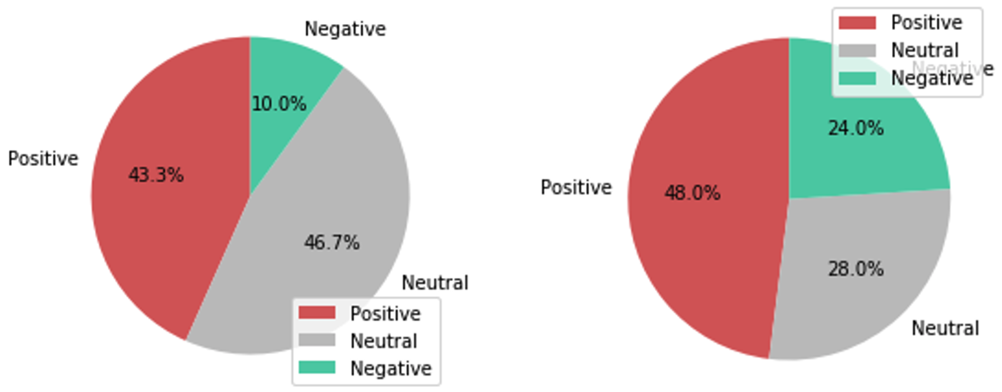
To determine the polarity for each sentence, we utilized the polarity scores from the VADER tool output [34]. This approach produces four scores: negative, positive, neutral, and the compound score, which is the total of all negative, positive, and neutral lexical evaluations. Using StockTwits data, the majority of tweets were discovered to be neutral. In particular, 46.7% of tweets were neutral, 43.3% were positive, and 10.0% were negative. This observation suggests that the majority of users are neutral to positive about buying or selling Microsoft shares. However, when examining Twitter statistics, the majority of tweets were positive. In particular, 48.0% of tweets were positive, 28.0% were neutral, and 24.0% were negative (Figure 3).
3.3.2. TextBlob
3.4. Algorithmic Tuning
To estimate the data patterns and make prediction computations, we facilitated ML development by utilizing a variety of python modules from the ‘scikit-learn’ library [38]. For the development of KNN, we used the ‘KneighborsClassifier’ class and its methods from the ‘sklearn.neighbors’ module. The number of neighbors was set to five. It was the best choice after running five trials, arbitrarily setting different k values (1, 3, 5, 7 and 9) and the default values for five-fold cross validation using the ‘KFold’ class from the ‘sklearn.model_selection’ module for dataset training and validation [40]. In addition, we implemented SVM with the help of the ‘SVC’ class and its methods from the ‘sklearn.svm’ module using a linear kernel for the decision boundary. The use of linear kernel provides better results for stock market forecasting problems in comparison with the other types of kernel, especially when the number of data points is not so high [41]. For the application of LR, we utilized the ‘LogisticRegression’ class and its methods from the ‘sklearn.linear_model’ module, while the NB algorithm was applied with the help of the ‘MinMaxScaler’ class and its methods from the ‘sklearn.preprocessing’ module. Furthermore, we employed the DT algorithm with the ‘tree.DecisionTreeClassifier’ class and its methods from the ‘sklearn.tree’ module and the RF algorithm with the ‘RandomForestClassifier’ class and its methods from the ‘sklearn.ensemble’ module. The last one is the MLP algorithm. The class used was the ‘MLPClassifier’, along with its methods from the ‘sklearn.neural_network’ module. The number of hidden layers was set to two and the number of neurons was 40 and 40, respectively [42]. These parameters were tested to be the optimal after performing an exhaustive grid search hyperparameter tuning with the ‘GridSearchCV’ class and its methods from the ‘sklearn.model_selection’ module.
3.5. Model Validation
To evaluate the SMP model, the train/test split method was applied in this paper. The train/test split method is a validation technique where the entire dataset is divided into training and test sets in order to estimate the performance of the ML algorithms. For both training and test sets, we calculated the F-score and AUC [33] to evaluate the performance for each implemented classification algorithm (KNN, SVM, LR, NB, DT, RF and MLP). The Pareto Principle has been utilized where the number of splits was set to 20, indicating that the 20% of the dataset will be tested and the 80% of the dataset will be used as a training set [43].
The test set was comprised of data where the period ranged from 10 October 2020 to 31 October 2020, while the training set included data from 16 July 2020 to 9 October 2020. The train/test split was employed across all the ML algorithms. In order to validate our results, we used the python class named ‘train_test_split‘ from the ‘sklearn.model_selection’ module of the ‘scikit-learn’ library [38]. The input features and the target variable were the input of the ‘train_test_split‘ method, as well as the size of the test set, which was set to 20% of the entire dataset.
4. Results
Following the collection and preparation of data, as well as the development of the approach, the next stage is to evaluate how efficient and suitable our model is for predicting Microsoft stock price. Employing captions we present F-score and AUC values to assess our model’s ability to forecast stock prices.
4.1. Model
We employed a binary classification, since it produces better results than a continuous classification [44]. The sentiment value, low and high price, volume, and adjusted price are all input features. The target feature, on the other hand, is the stock change, which has two separate values (−1 and 1). Therefore, it has two numbers that describe the state of either selling or buying the stock.
Table 5 shows the distribution of the target variable for StockTwits and Twitter, as well as the SA tools TextBlob and VADER. In all four scenarios, the number of buyers outnumbers the number of sellers, suggesting that most individuals prefer to acquire Microsoft stock and sell it less frequently.
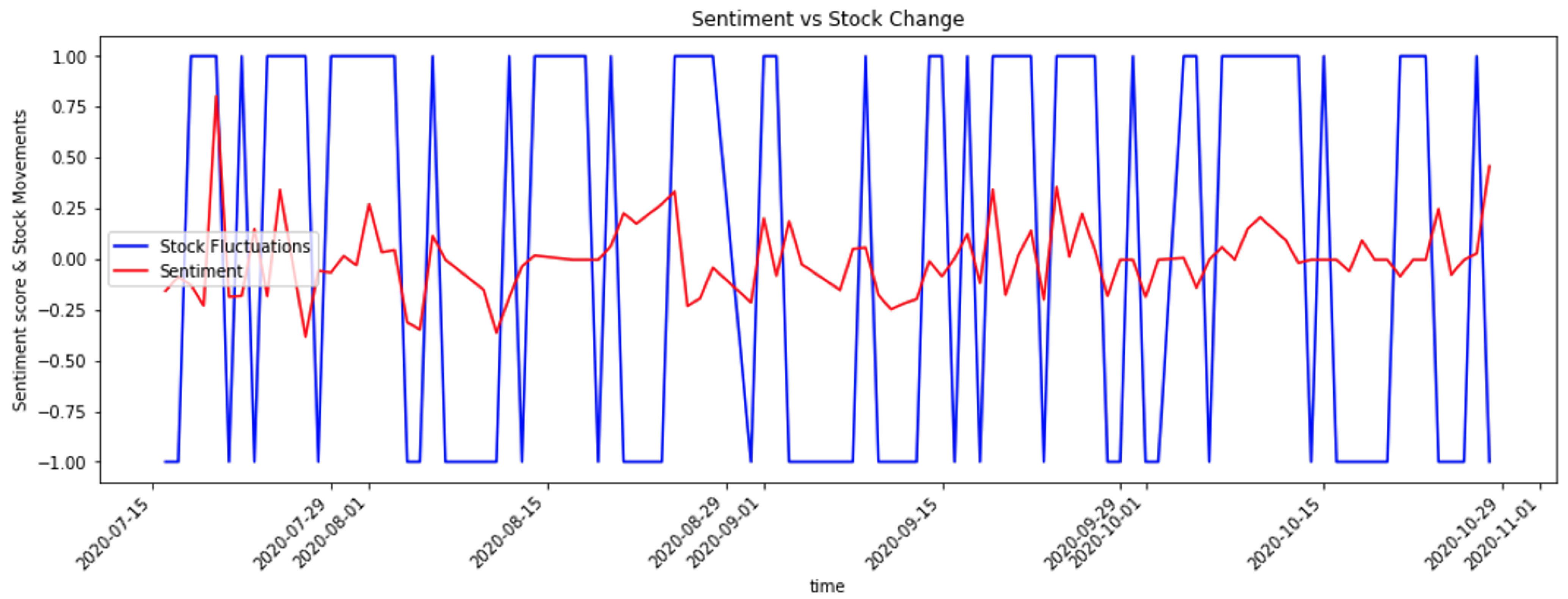
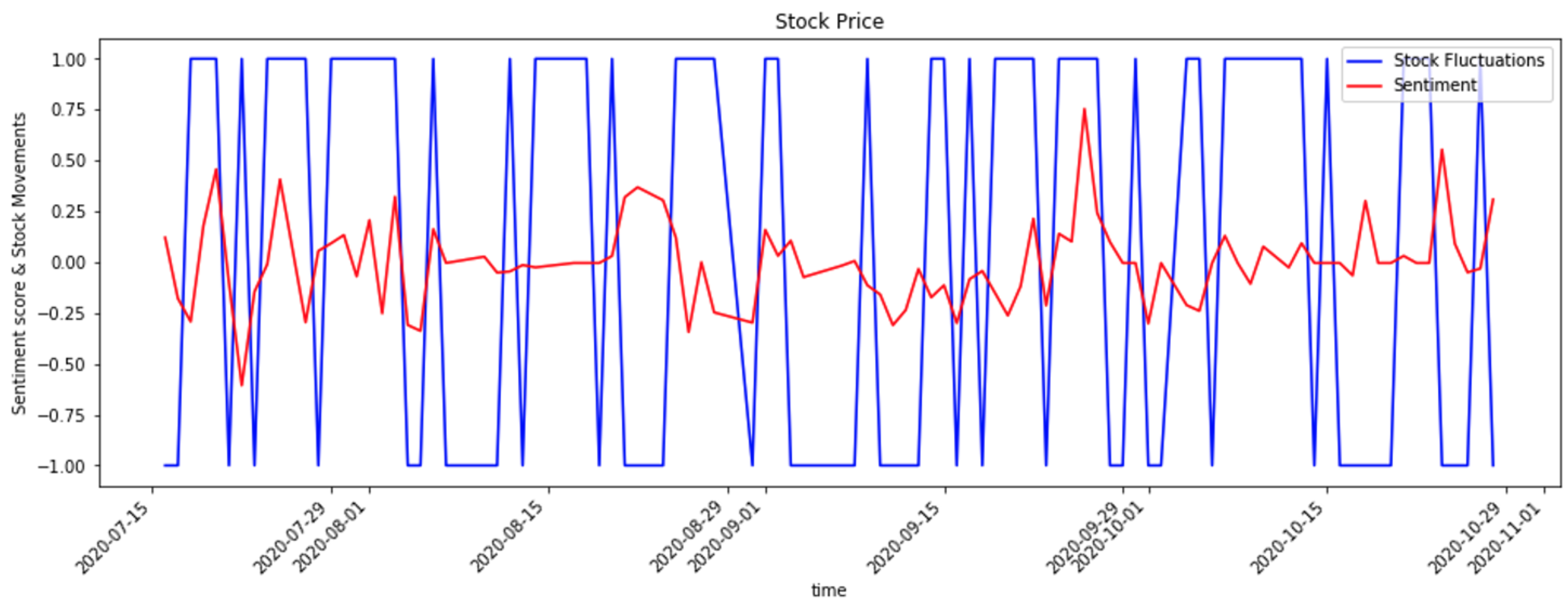
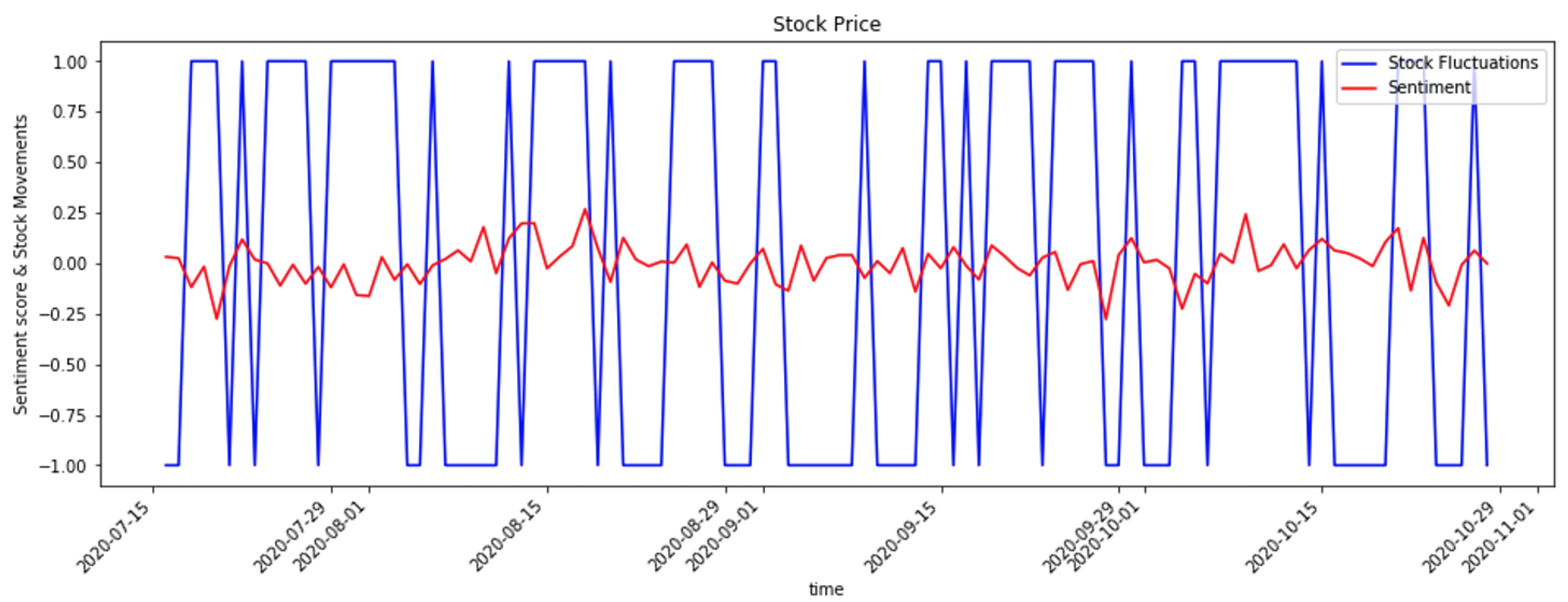
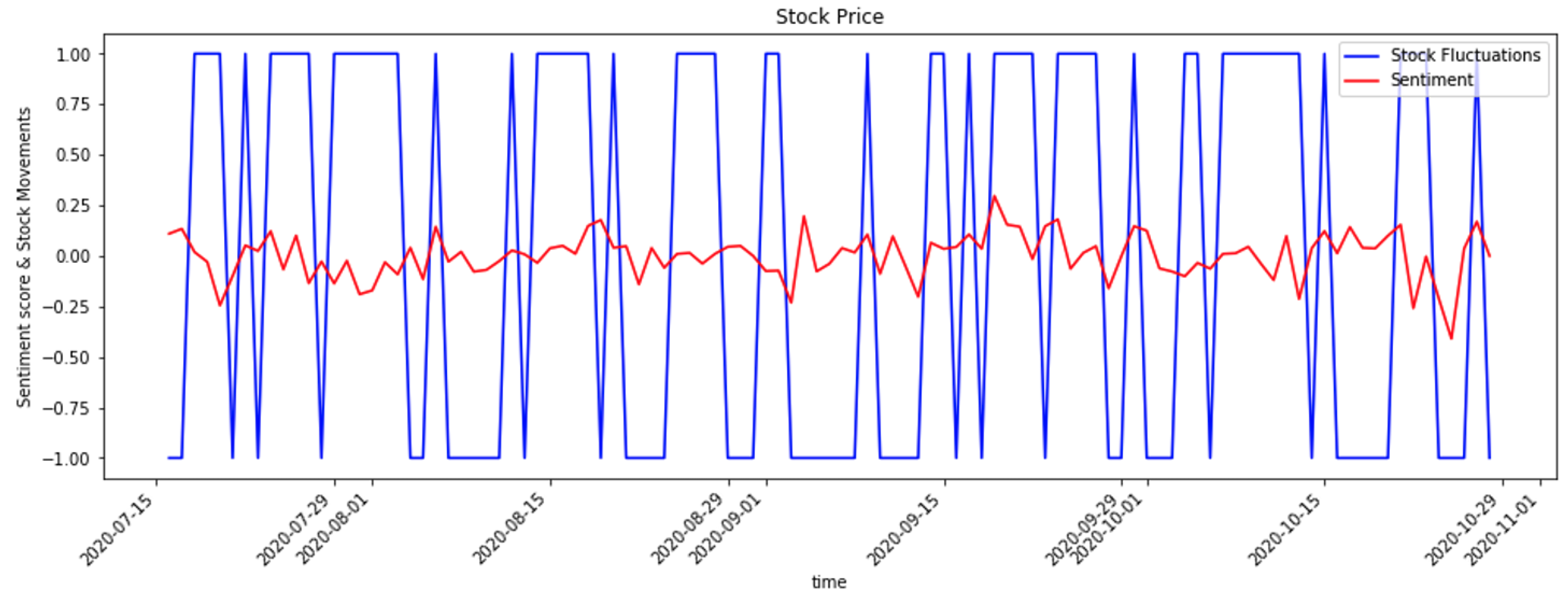
The input and target variables are displayed over time in the figures below. The blue line shows the target variable, which is the change in the stock price, and the red line indicates the input variable, which is public opinion towards the Microsoft stock.
Particularly, Figure 5 shows that the two lines are associated from July to August. When sentiment is favorable, stock change rises, meaning that when individuals are optimistic, they tend to purchase Microsoft shares. From September through October, the trend is similar to the preceding period, though with some notable variances.
On the other hand, there is no apparent trend for August (Figure 6). Instead, it appears that sentiment in July is tied to market movement. When the mood is good, stock exchange prices rise, and vice versa. The two lines are connected for several days in September and October, although there are many variances.
When Twitter data are utilized and evaluated with the TextBlob and VADER, as illustrated in Figure 7 and Figure 8, the majority of tweets have a neutral sentiment. There are many highs and lows that are very near to zero. This suggests that utilizing Twitter data to anticipate stock prices may be unreliable, as emotion and stock movement are unrelated.
4.2. Performance
This section shows the outcomes of employing VADER and TextBlob as Twitter and StockTwits SA tools, respectively. Two measures were utilized to assess the proposed model: F-score and AUC. The F-score is a measure of a model’s accuracy and predictability. AUC is defined as the area under the curve, and is formed by contrasting the true-positive rate against the false-positive rate. It describes the model’s discriminating power, as well as its ability to predict whether the stock price will increase or decline [33].
According to Table 6, Table 7, Table 8 and Table 9 we make the following observations. The F-scores of our ML models vary from 53.8% to 68.7% for the ‘StockTwits with TextBlob’ dataset, while the AUC areas range from 40% to 53.3% (Table 6). We are equally concerned about true positives and true negatives, since we want to anticipate both positive and negative increases in Microsoft’s share value. As a result, we use the F-score and the AUC as assessment measures, which are profoundly different. SVM has the highest F-score of 68.7% and the highest AUC of 53.3%. Similarly, NB performed well, with an F-score of 66.7% and an AUC of 51%.
According to Table 7 we observe that the F-score fluctuates from 45.5% to 68%, while the AUC ranges from 40% to 55%. SVM and LR achieve the best F-score, which is 68%. Their AUC is 55% and 54.7%, respectively. The next two best ML algorithms are NB and MLP, presenting an F-score equal to 66.7% and an AUC equal to 50%.
In the case of the ‘Twitter with TextBlob’ dataset (Table 8), the F-score varies from 54.1% to 75%. The best F-score is 75%, achieved by SVM; the second best is 74.3%, achieved by MLP; and the third best is 72%, achieved by KNN and DT. In addition, AUC values can be as high as 68%. Their percentages vary from 44% to 68%. The best AUC values are observed in KNN and DT, reaching 68%.
Finally, the F-score for the ‘Twitter with VADER’ dataset varies from 58% to 76.3% (Table 9). SVM has the greatest performance (76.3%), with LR coming in second with 70.1%. AUC, on the other hand, varies from 46% to 67%. SVM has the highest discriminating power of 67%, whereas LR has the second highest at 63.2%.
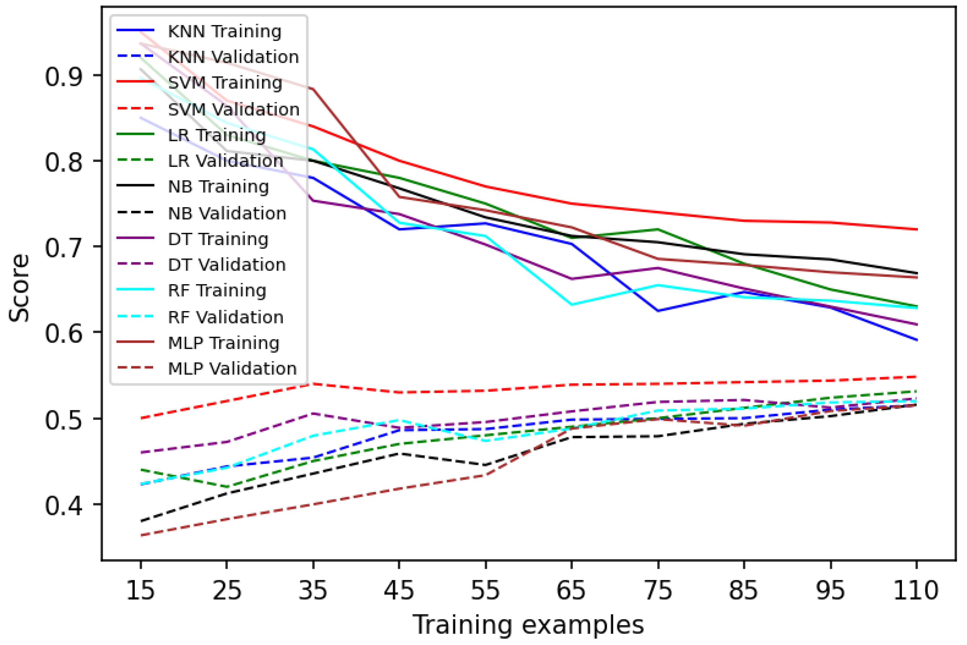
Next, it should be noted that Table 10 and Table 11 and Figure 9 refer to the average values of training/validation score, training/validation learning curve and training/validation time of all datasets (’StockTwits with TextBlob’, ’StockTwits with VADER’, ’Twitter with TextBlob’ and ’Twitter with VADER’) for all models (KNN, SVM, LR, NB, DT, RF and MLP) using F-score for training and AUC for validation. According to Table 10, SVM exhibits the best results, with a 72% average training score and a 54.83% validation score.
Finally, according to Table 11, it is observed that the LR resulted in the quickest training (2.26 s) and validation times (0.45 s), followed by the SVM with 3.55 s for training and 0.89 s for validation. On the other hand, the MLP is the slowest algorithm in terms of training and validation times, with values of 21.23 and 9.11 s, respectively.
5. Conclusions
5.1. Discussion
In this study, we addressed the subject of SMP utilizing ML approaches with SA. We experimented with Twitter and StockTwits, as well as financial data. Two SA tools, TextBlob and VADER, were utilized to analyze the sentiment of microblogging data. The novelty of this approach can be attributed to the integration of multiple SA and ML methods. We also highlight the importance of SM microblogging data and public sentiment as extra features for SMP. After performing data preprocessing, we assessed our model’s performance in four situations (TextBlob with either Twitter or StockTwits data, and VADER with either Twitter or StockTwits data) using seven ML algorithms, including KNN, SVM, LR, NB, DT, RF, and MLP. The model was evaluated using two metrics: the F-score and the AUC. The actual prediction power was evaluated from 10 October 2020 to 31 October 2020, demonstrating possible real-world consequences for forecasting Microsoft’s stock price movement.
According to Table 12, when utilizing the ‘StockTwits with TextBlob’ dataset, SVM performs best with an F-score of 68.7% and an AUC of 53.3%. This algorithm’s prediction was correct for ten days, during which stock values climbed.
Utilizing the ‘StockTwits with VADER’ dataset, SVM and LR produced the best F-score (68%) and predictive ability (the prediction was right for 10 days, projecting that Microsoft stock prices would rise). Furthermore, these algorithms produced high AUC values: 55% for SVM and 54.75% for LR, respectively.
When using the ‘Twitter with TextBlob’ dataset, SVM got the highest F-score (75%), effectively predicting the outcome for 13 days. However, RF with an F-score of 69.6% appears to produce the most accurate forecasts, as it anticipated properly that for 16 days, the stock prices would rise. Moreover, KNN and DT have the highest discriminating power, with AUC scores of 68% and F-scores of 72%.
Finally, while employing the ‘Twitter with VADER’ dataset, SVM demonstrated the greatest F-score (76.3%) and AUC (67%). Admittedly, SVM provided the most accurate forecasts throughout a 15-day period, during which the anticipated prices climbed.
To summarize, the utilization of Twitter data, and specifically the ‘Twitter with VADER’ dataset, yielded the highest predictive (F-score, 76.3%) and second best discriminating power (AUC, 67%). This suggests that our model can forecast the true-positive and true-negative points properly. The ‘Twitter with TextBlob’ dataset has the second greatest overall predictive power, with an F-score of 75% utilizing the SVM algorithm and an AUC value of 68% utilizing the KNN and DT algorithms. As a consequence, it was determined that the Twitter dataset produced findings with the greatest overall values for F-score and AUC. Lastly, Microsoft stock price movements were accurately anticipated to rise on the majority of days.
5.2. Limitations
A few factors might jeopardize the validity of our findings. Firstly, Python packages such as TextBlob and VADER produce incorrect sentiment scores for a number of tweets. For example, in the presence of sarcasm, they frequently misinterpret a bad tweet as a good one and vice versa, resulting in an improper training set.
Another risk to the accuracy of our results is the presence of spam accounts, false accounts, and bots that generate Twitter and StockTwits data. As a result, the dissemination of false information and an incorrectly estimated sentiment may be stored in our dataset. Furthermore, it was discovered that for a specific day, although sentiment might be positive, stock movement might be moving downwards.
Lastly, the presented assessment metrics may be deemed limiting. Nonetheless, due to our preliminary findings in [45], we excluded publishing further accuracy metrics. There is a class imbalance problem in the data, as seen in Table 5. In all four analyzed examples, the number of buyers outnumbers the number of sellers, indicating that most individuals prefer to purchase Microsoft stocks and just a few choose to sell them. For unbalanced data, F-score and AUC are suitable metrics [46].
5.3. Future Work
A number of components of this study might be improved in the future. Collecting tweets from accounts with a large number of followers, for example, who have a major effect on market movements, may increase model performance. It is also possible to investigate the elimination of false Twitter accounts, as they might distort sentiment computation. Additionally, exploiting more data and trade dates can increase model performance. Furthermore, to boost accuracy, we may pick features that are highly connected to the target variable, or we could aggregate all of the features and then choose the most efficient classifier.
Finally, we may use several ML techniques to compute the sentiment score. It could be more accurate if we trained and tested our Twitter data instead of using a pre-packaged library. TextBlob and VADER, for instance, may misinterpret a positive text as negative, resulting in an incorrect sentiment rate. As a result, training and testing our data might aid in the improvement of the proposed approach.
Author Contributions
Conceptualization, P.K., C.N. and C.T.; methodology, P.K. and C.N.; software, C.N. and P.K.; validation, P.K. and C.T.; formal analysis, P.K.; investigation, P.K., C.N. and C.T.; resources, C.N.; data curation, C.N.; writing—original draft preparation, P.K.; writing—review and editing, P.K. and C.T.; visualization, P.K. and C.N.; supervision, C.T.; project administration, C.T. and P.K. All authors have read and agreed to the published version of the manuscript.
Funding
This research received no external funding.
Institutional Review Board Statement
Not applicable.
Informed Consent Statement
Not applicable.
Data Availability Statement
Data partly available in captions.
Conflicts of Interest
Researchers in School of Science and Technology, International Hellenic University.
Abbreviations
The following abbreviations are used in this manuscript:
| AUC | Area Under Curve; |
| DM | Data Mining; |
| DT | Decision Tree; |
| KNN | K-nearest Neighbors; |
| LR | Logistic Regression; |
| ML | Machine Learning; |
| MLP | Multilayer Perceptron; |
| NN | Neural Network; |
| RF | Random Forest; |
| SA | Sentiment Analysis; |
| SMP | Stock Market Prediction; |
| SVM | Support Vector Machine. |
References
- Billah, M.; Waheed, S.; Hanifa, A. Stock market prediction using an improved training algorithm of neural network. In Proceedings of the 2016 2nd International Conference on Electrical, Computer & Telecommunication Engineering (ICECTE), Rajshahi, Bangladesh, 8–10 December 2016; pp. 1–4. [Google Scholar]
- Khedr, A.E.; Yaseen, N. Predicting stock market behavior using data mining technique and news sentiment analysis. Int. J. Intell. Syst. Appl. 2017, 9, 22. [Google Scholar] [CrossRef]
- Rousidis, D.; Koukaras, P.; Tjortjis, C. Social media prediction: A literature review. Multimed. Tools Appl. 2020, 79, 6279–6311. [Google Scholar] [CrossRef]
- Gurjar, M.; Naik, P.; Mujumdar, G.; Vaidya, T. Stock market prediction using ANN. Int. Res. J. Eng. Technol. 2018, 5, 2758–2761. [Google Scholar]
- Huang, Y.; Capretz, L.F.; Ho, D. Machine learning for stock prediction based on fundamental analysis. In Proceedings of the 2021 IEEE Symposium Series on Computational Intelligence (SSCI), Orlando, FL, USA, 5–7 December 2021; pp. 1–10. [Google Scholar]
- Smailović, J.; Grčar, M.; Lavrač, N.; Žnidaršič, M. Predictive sentiment analysis of tweets: A stock market application. In International Workshop on Human-Computer Interaction and Knowledge Discovery in Complex, Unstructured, Big Data; Springer: Berlin/Heidelberg, Germany, 2013; pp. 77–88. [Google Scholar]
- Koukaras, P.; Tjortjis, C.; Rousidis, D. Social Media Types: Introducing a Data Driven Taxonomy; Springer: Vienna, Austria, 2020; Volume 102, pp. 295–340. [Google Scholar] [CrossRef]
- Koukaras, P.; Tjortjis, C. Social Media Analytics, Types and Methodology. In Machine Learning Paradigms; Springer: Cham, Switzerland, 2019; pp. 401–427. [Google Scholar] [CrossRef]
- Nasukawa, T.; Yi, J. Sentiment analysis: Capturing favorability using natural language processing. In Proceedings of the 2nd International Conference on Knowledge Capture, New York, NY, USA, 23–25 October 2003; pp. 70–77. [Google Scholar]
- Kordonis, J.; Symeonidis, S.; Arampatzis, A. Stock price forecasting via sentiment analysis on Twitter. In Proceedings of the 20th Pan-Hellenic Conference on Informatics, New York, NY, USA, 10–12 November 2016; pp. 1–6. [Google Scholar]
- Pagolu, V.S.; Reddy, K.N.; Panda, G.; Majhi, B. Sentiment analysis of Twitter data for predicting stock market movements. In Proceedings of the 2016 International Conference on Signal Processing, Communication, Power and Embedded System (SCOPES), Paralakhemundi, India, 3–5 October 2016; pp. 1345–1350. [Google Scholar]
- Mittal, A.; Goel, A. Stock Prediction Using Twitter Sentiment Analysis. In Standford Univ. CS229; 2011; Volume 15, p. 2352. Available online: http://cs229.stanford.edu/proj2011/GoelMittal-StockMarketPredictionUsingTwitterSentimentAnalysis.pdf (accessed on 17 March 2022).
- Hamed, A.R.; Qiu, R.; Li, D. Analysis of the relationship between Saudi twitter posts and the Saudi stock market. In Proceedings of the 2015 IEEE Seventh International Conference on Intelligent Computing and Information systems (ICICIS), Cairo, Egypt, 12–14 December 2015; pp. 660–665. [Google Scholar]
- Batra, R.; Daudpota, S.M. Integrating StockTwits with sentiment analysis for better prediction of stock price movement. In Proceedings of the 2018 International Conference on Computing, Mathematics and Engineering Technologies (iCoMET), Sukkur, Pakistan, 3–4 March 2018; pp. 1–5. [Google Scholar]
- Gupta, R.; Chen, M. Sentiment analysis for stock price prediction. In Proceedings of the 2020 IEEE Conference on Multimedia Information Processing and Retrieval (MIPR), Shenzhen, China, 6–8 August 2020; pp. 213–218. [Google Scholar]
- Sun, T.; Wang, J.; Zhang, P.; Cao, Y.; Liu, B.; Wang, D. Predicting stock price returns using microblog sentiment for chinese stock market. In Proceedings of the 2017 3rd International Conference on Big Data Computing and Communications (BIGCOM), Chengdu, China, 10–11 August 2017; pp. 87–96. [Google Scholar]
- Hatefi Ghahfarrokhi, A.; Shamsfard, M. Tehran stock exchange prediction using sentiment analysis of online textual opinions. Intell. Syst. Account. Financ. Manag. 2020, 27, 22–37. [Google Scholar] [CrossRef] [Green Version]
- Wu, S.; Liu, Y.; Zou, Z.; Weng, T.H. S_I_LSTM: Stock price prediction based on multiple data sources and sentiment analysis. Connect. Sci. 2022, 34, 44–62. [Google Scholar] [CrossRef]
- Zhao, B.; He, Y.; Yuan, C.; Huang, Y. Stock market prediction exploiting microblog sentiment analysis. In Proceedings of the 2016 International Joint Conference on Neural Networks (IJCNN), Vancouver, BC, Canada, 24–29 July 2016; pp. 4482–4488. [Google Scholar]
- Deng, S.; Huang, Z.J.; Sinha, A.P.; Zhao, H. The interaction between microblog sentiment and stock return: An empirical examination. MIS Q. 2018, 42, 895–918. [Google Scholar] [CrossRef]
- Oliveira, N.; Cortez, P.; Areal, N. The impact of microblogging data for stock market prediction: Using Twitter to predict returns, volatility, trading volume and survey sentiment indices. Expert Syst. Appl. 2017, 73, 125–144. [Google Scholar] [CrossRef] [Green Version]
- Wang, Y. Stock market forecasting with financial micro-blog based on sentiment and time series analysis. J. Shanghai Jiaotong Univ. (Sci.) 2017, 22, 173–179. [Google Scholar] [CrossRef]
- Yan, D.; Zhou, G.; Zhao, X.; Tian, Y.; Yang, F. Predicting stock using microblog moods. China Commun. 2016, 13, 244–257. [Google Scholar] [CrossRef]
- Neelamegam, S.; Ramaraj, E. Classification algorithm in data mining: An overview. Int. J. P2p Netw. Trends Technol. 2013, 4, 369–374. [Google Scholar]
- Koukaras, P.; Rousidis, D.; Tjortjis, C. An Introduction to Information Network Modeling Capabilities, Utilizing Graphs. In Communications in Computer and Information Science; Springer: Cham, Switzerland, 2021; Volume 1355 CCIS, pp. 134–140. [Google Scholar] [CrossRef]
- Guo, G.; Wang, H.; Bell, D.; Bi, Y.; Greer, K. KNN model-based approach in classification. In Proceedings of the OTM Confederated International Conferences “On the Move to Meaningful Internet Systems”; Springer: Berlin/Heidelberg, Germany, 2003; pp. 986–996. [Google Scholar]
- Qi, X.; Silvestrov, S.; Nazir, T. Data classification with support vector machine and generalized support vector machine. In Proceedings of the AIP Conference Proceedings; AIP Publishing LLC: Melville, NY, USA, 2017; Volume 1798, p. 020126. [Google Scholar]
- Kleinbaum, D.G.; Dietz, K.; Gail, M.; Klein, M.; Klein, M. Logistic Regression; Springer: Berlin/Heidelberg, Germany, 2002. [Google Scholar]
- Rish, I. An empirical study of the naive Bayes classifier. In Proceedings of the IJCAI 2001 Workshop on Empirical Methods in Artificial Intelligence, Seattle, WA, USA, 4–10 August 2001; Volume 3, pp. 41–46. [Google Scholar]
- Safavian, S.R.; Landgrebe, D. A survey of decision tree classifier methodology. IEEE Trans. Syst. Man Cybern. 1991, 21, 660–674. [Google Scholar] [CrossRef] [Green Version]
- Breiman, L. Random forests. Mach. Learn. 2001, 45, 5–32. [Google Scholar] [CrossRef] [Green Version]
- Pal, S.K.; Mitra, S. Multilayer perceptron, fuzzy sets, classifiaction. IEEE Trans. Neural Netw. 1992, 3, 683–697. [Google Scholar] [CrossRef] [PubMed]
- Sokolova, M.; Japkowicz, N.; Szpakowicz, S. Beyond accuracy, F-score and ROC: A family of discriminant measures for performance evaluation. In Australasian Joint Conference on Artificial Intelligence; Springer: Berlin/Heidelberg, Germany, 2006; pp. 1015–1021. [Google Scholar]
- Hutto, C.; Gilbert, E. Vader: A parsimonious rule-based model for sentiment analysis of social media text. In Proceedings of the International AAAI Conference on Web and Social Media, Ann Arbor, MI, USA, 1–4 June 2014; Volume 8, pp. 216–225. [Google Scholar]
- Loria, S. textblob Documentation, Release 0.15; Python Software Foundation: Wilmington, DE, USA, 2018; Volume 2, p. 269. [Google Scholar]
- Sanders, R. The Pareto principle its use and abuse. J. Bus. Ind. Mark. 1988, 3, 37. [Google Scholar] [CrossRef]
- Nann, S.; Krauss, J.; Schoder, D. Predictive analytics on public data-the case of stock markets. In Proceedings of the ECIS 2013 Completed Research (ECIS), Utrecht, The Netherlands, 5–8 June 2013. [Google Scholar]
- Buitinck, L.; Louppe, G.; Blondel, M.; Pedregosa, F.; Mueller, A.; Grisel, O.; Niculae, V.; Prettenhofer, P.; Gramfort, A.; Grobler, J.; et al. API design for machine learning software: Experiences from the scikit-learn project. In Proceedings of the ECML PKDD Workshop: Languages for Data Mining and Machine Learning, Prague, Czech Republic, 23–27 September 2013; pp. 108–122. [Google Scholar]
- Meijering, E. A chronology of interpolation: From ancient astronomy to modern signal and image processing. Proc. IEEE 2002, 90, 319–342. [Google Scholar] [CrossRef] [Green Version]
- Danil, M.; Efendi, S.; Sembiring, R.W. The Analysis of Attribution Reduction of K-Nearest Neighbor (KNN) Algorithm by Using Chi-Square. J. Phy. Conf. Ser. 2019, 1424, 012004. [Google Scholar] [CrossRef]
- Upadhyay, V.P.; Panwar, S.; Merugu, R.; Panchariya, R. Forecasting stock market movements using various kernel functions in support vector machine. In Proceedings of the International Conference on Advances in Information Communication Technology & Computing, New York, NY, USA, 12–13 August 2016; pp. 1–5. [Google Scholar]
- Moghaddam, A.H.; Moghaddam, M.H.; Esfandyari, M. Stock market index prediction using artificial neural network. J. Econ. Financ. Adm. Sci. 2016, 21, 89–93. [Google Scholar] [CrossRef] [Green Version]
- Dunford, R.; Su, Q.; Tamang, E. The pareto principle. Plymouth Stud. Sci. 2014, 7, 140–148. [Google Scholar]
- Nabipour, M.; Nayyeri, P.; Jabani, H.; Shahab, S.; Mosavi, A. Predicting stock market trends using machine learning and deep learning algorithms via continuous and binary data; a comparative analysis. IEEE Access 2020, 8, 150199–150212. [Google Scholar] [CrossRef]
- Nousi, C.; Tjortjis, C. A Methodology for Stock Movement Prediction Using Sentiment Analysis on Twitter and StockTwits Data. In Proceedings of the 2021 6th South-East Europe Design Automation, Computer Engineering, Computer Networks and Social Media Conference (SEEDA-CECNSM), Preveza, Greece, 24–26 September 2021; pp. 1–7. [Google Scholar]
- Gurav, U.; Sidnal, N. Predict Stock Market Behavior: Role of Machine Learning Algorithms. In Intelligent Computing and Information and Communication; Springer: Berlin, Germany, 2018; pp. 383–394. [Google Scholar]
Figure 1.
Flowchart of research design.

Figure 2.
Microsoft stock open and close values.

Figure 3.
Sentiment analysis for StockTwits (left piechart) and Twitter (right piechart) datasets using VADER.
Figure 3.
Sentiment analysis for StockTwits (left piechart) and Twitter (right piechart) datasets using VADER.

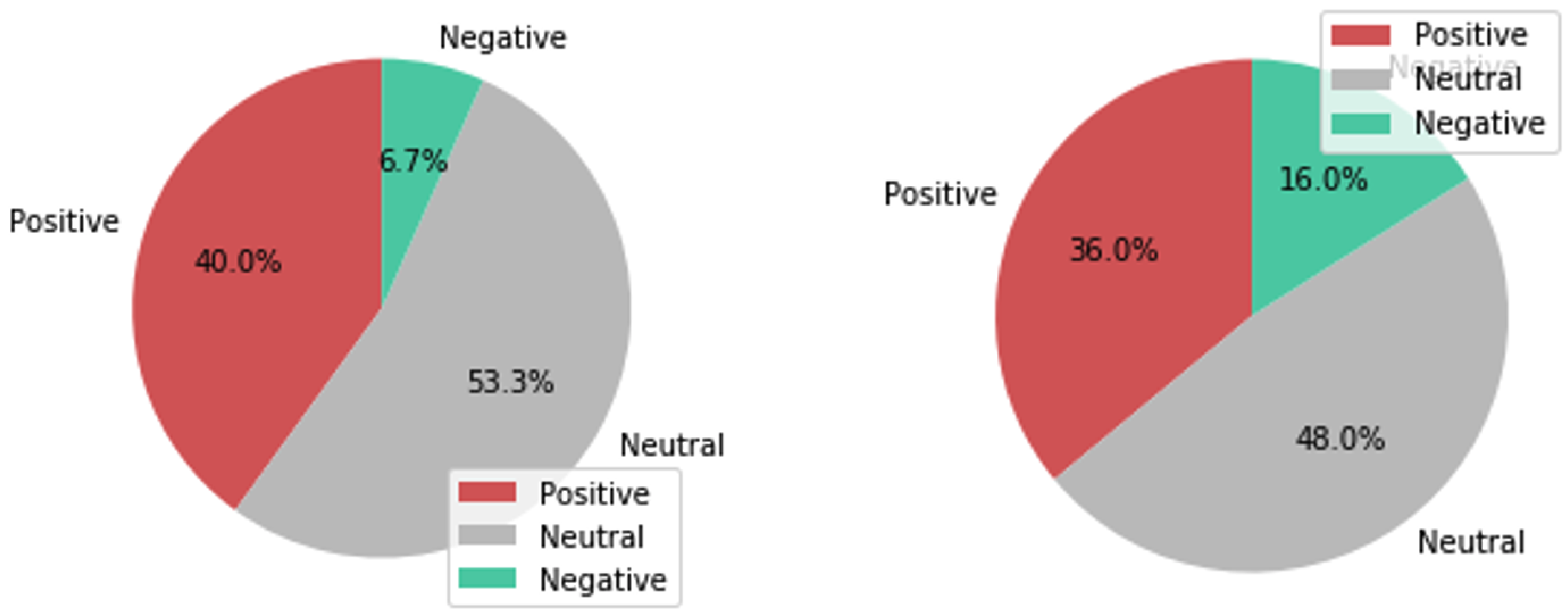
Figure 4.
Sentiment analysis for StockTwits (left piechart) and Twitter (right piechart) datasets using TextBlob.
Figure 4.
Sentiment analysis for StockTwits (left piechart) and Twitter (right piechart) datasets using TextBlob.

Figure 5.
Sentiment and stock change for ‘StockTwits with TextBlob’ dataset.

Figure 6.
Sentiment and stock change for ‘StockTwits with VADER’ data set.

Figure 7.
Sentiment & Stock Change for ‘Twitter with TextBlob’ data set.

Figure 8.
Sentiment & Stock Change for ‘Twitter with VADER’ data set.

Figure 9.
Average learning curve for all models.


Table 1.
Sample of Twitter data.
| Id | Keyword | Text | Date |
|---|---|---|---|
| 74509 | #Microsoft | Just went live! gamerlife xbox livestream livestr | 22 September 2020 |
| 11533 | #Microsoft | Azure Blob versioning public preview region expans… | 16 July 2020 |
| 77325 | #Microsoft | Both boys give their hot taco takes on Microsoft’s… | 25 September 2020 |
| 12557 | #Microsoft | Process Monitor for Linux:Microsoft has released… | 17 July 2020 |
| 79373 | #Microsoft | Is process optimization part of your digital strat… | 29 September 2020 |
Table 2.
Sample of StockTwits data.
| Id | Text | Date |
|---|---|---|
| 245 | $MSFT Citigroup Maintains to Neutral: PT $ 216.00 | 16 July 2020 |
| 246 | $MSFT Hopefully a good day… its gonna take every… | 16 July 2020 |
| 247 | $MSFT with all those upgrades of ratings and partn | 16 July 2020 |
| 248 | $NFLX $FB $GLD $VXX $MSFT Thanks to the for help… | 16 July 2020 |
| 249 | $MSFT credit Suisse raises microsoft price | 16 July 2020 |
Table 3.
Sample of Yahoo! Finance data.
| Open ($) | High ($) | Low ($) | Close ($) | Adj Close ($) | Volume | Date |
|---|---|---|---|---|---|---|
| 205.00 | 212.30 | 203.01 | 211.60 | 208.36 | 36,884,800 | 20 July 2020 |
| 213.66 | 213.94 | 208.03 | 208.75 | 205.55 | 37,990,400 | 21 July 2020 |
| 209.20 | 212.30 | 208.39 | 211.75 | 208.51 | 49,605,700 | 22 July 2020 |
| 207.19 | 210.92 | 202.15 | 202.54 | 199.44 | 67,457,000 | 23 July 2020 |
| 200.42 | 202.86 | 197.51 | 201.30 | 198.22 | 39,827,000 | 24 July 2020 |
Table 4.
Outlier distribution.
| Dataset | Outliers |
|---|---|
| Twitter with VADER | 19.7% |
| Twitter with TextBlob | 9.6% |
| StockTwits with VADER | 27.1% |
| StockTwits with TextBlob | 27.3% |
Table 5.
Stock movement distribution per data set.
| Dataset | Buy Count | Sell Count |
|---|---|---|
| StockTwits with TextBlob | 51 | 39 |
| StockTwits with VADER | 49 | 42 |
| Twitter with TextBlob | 55 | 45 |
| Twitter with VADER | 53 | 46 |
Table 6.
Algorithmic performance for ‘StockTwits with TextBlob’ dataset.
| Model | F-Score (%) | AUC (%) |
|---|---|---|
| KNN | 53.8 | 40 |
| SVM | 68.7 | 53.3 |
| LR | 59.9 | 44.6 |
| NB | 66.7 | 51 |
| DT | 61.5 | 50 |
| RF | 61.5 | 50 |
| MLP | 56 | 45 |
Table 7.
Algorithmic performance for ‘StockTwits with VADER’ dataset.
| Model | F-Score (%) | AUC (%) |
|---|---|---|
| KNN | 45.5 | 40 |
| SVM | 68 | 55 |
| LR | 68 | 54.7 |
| NB | 66.7 | 50 |
| DT | 52.2 | 45 |
| RF | 58.8 | 45 |
| MLP | 66.7 | 50 |
Table 8.
Algorithmic performance for ‘Twitter with TextBlob’ dataset.
| Model | F-Score (%) | AUC (%) |
|---|---|---|
| KNN | 72 | 68 |
| SVM | 75 | 44 |
| LR | 54.1 | 50 |
| NB | 70.3 | 50 |
| DT | 72 | 68 |
| RF | 69.6 | 64 |
| MLP | 74.3 | 50 |
Table 9.
Algorithmic performance for ‘Twitter with VADER’ data set.
| Model | F-Score (%) | AUC (%) |
|---|---|---|
| KNN | 65.2 | 58 |
| SVM | 76.3 | 67 |
| LR | 70.1 | 63.2 |
| NB | 63.9 | 55.3 |
| DT | 58 | 46 |
| RF | 61.5 | 49 |
| MLP | 68.6 | 61 |
Table 10.
Average training and validation score for all models.
| Model | Training Score (%) | Validation Score (%) |
|---|---|---|
| KNN | 59.13 | 51.5 |
| SVM | 72 | 54.83 |
| LR | 63.03 | 53.13 |
| NB | 66.9 | 51.58 |
| DT | 60.93 | 52.3 |
| RF | 62.85 | 52 |
| MLP | 66.4 | 51.5 |
Table 11.
Average training and validation time for all models.
| Model | Training Time (s) | Validation Time (s) |
|---|---|---|
| KNN | 4.34 | 1.12 |
| SVM | 3.55 | 0.89 |
| LR | 2.26 | 0.45 |
| NB | 6.23 | 2.31 |
| DT | 9.89 | 2.98 |
| RF | 10.29 | 3.13 |
| MLP | 21.23 | 9.11 |
Table 12.
Best results per dataset.
| Dataset | Method/F-Score | Method/AUC |
|---|---|---|
| ‘StockTwits with TextBlob’ | SVM/68.7% | SVM/53.3% |
| ‘StockTwits with VADER’ | SVM & LR/68% | SVM/55% |
| ‘Twitter with TextBlob’ | SVM/75% | KNN & DT/68% |
| ‘Twitter with VADER’ | SVM/76.3% | SVM/67% |
Publisher’s Note: MDPI stays neutral with regard to jurisdictional claims in published maps and institutional affiliations. |
© 2022 by the authors. Licensee MDPI, Basel, Switzerland. This article is an open access article distributed under the terms and conditions of the Creative Commons Attribution (CC BY) license (https://creativecommons.org/licenses/by/4.0/).
Share and Cite
MDPI and ACS Style
Koukaras, P.; Nousi, C.; Tjortjis, C. Stock Market Prediction Using Microblogging Sentiment Analysis and Machine Learning. Telecom 2022, 3, 358-378. https://0-doi-org.brum.beds.ac.uk/10.3390/telecom3020019
AMA Style
Koukaras P, Nousi C, Tjortjis C. Stock Market Prediction Using Microblogging Sentiment Analysis and Machine Learning. Telecom. 2022; 3(2):358-378. https://0-doi-org.brum.beds.ac.uk/10.3390/telecom3020019
Chicago/Turabian StyleKoukaras, Paraskevas, Christina Nousi, and Christos Tjortjis. 2022. "Stock Market Prediction Using Microblogging Sentiment Analysis and Machine Learning" Telecom 3, no. 2: 358-378. https://0-doi-org.brum.beds.ac.uk/10.3390/telecom3020019