Design Optimization and Sizing for Fly-Gen Airborne Wind Energy Systems

Abstract

Traditional on-shore horizontal-axis wind turbines need to be large for both performance reasons (e.g., clearing ground turbulence and reaching higher wind speeds) and for economic reasons (e.g., more efficient land use, lower maintenance costs, and fewer controllers and grid attachments) while their efficiency is scale and mass independent. Airborne wind energy (AWE) system efficiency is a function of system size and AWE system operating altitude is less directly coupled to system power rating. This paper derives fly-gen AWE system parameters from small number of design parameters, which are used to optimize a design for energy cost. This paper then scales AWE systems and optimizes them at each scale to determine the relationships between size, efficiency, power output, and cost. The results indicate that physics and economics favor a larger number of small units, at least offshore or where land cost is small.

1. Introduction

1.1. Airborne Wind Energy

Offshore wind energy has advantages in resource availability over onshore wind and has better load matching than solar energy [1,2]. Offshore wind is also more expensive than either [3,4]. Airborne wind energy (AWE) is a technology with the potential to harvest abundant wind resources located over deep water less expensively than current wind energy technologies [5]. It is therefore a good candidate for economically assisting with decarbonization and helping to mitigate global warming.

AWE uses tethered aircraft to harvest wind energy. The combination of aerodynamic forces and tether tension propel the aircraft perpendicular to the wind, analogous to a wind turbine blade. Higher altitude winds are faster and more reliable than surface-level winds [6], and using a tether rather than a tower makes it easier to increase operating altitude. While the blades and tower of a conventional wind turbine must be designed for significant bending and compressive loads, AWE systems are anchored to the ground by a tether and can use a bridle to support the aircraft wing, resulting in significantly less structural weight for the same power production. A lower weight system with a simpler foundation promises logistical benefits such as lower capital costs, transportation costs, maintenance costs, easier installation for offshore systems, and a lower cost of energy.

Two forms of AWE were proposed by Miles Loyd in 1980. Ground-gen AWE systems operate by reeling the tether out under high load, producing power from regenerative braking on the winch, and then reeling back in under lower load. Fly-gen AWE system use turbines on the aircraft to harvest wind power while moving at high crosswind speeds and transmit that power to the ground via an electrified tether [7]. The turbines on board the aircraft used for fly-gen AWE systems experience an airspeed significantly higher than the wind speed, allowing smaller, faster-spinning turbines and lighter, more energy-dense power systems than comparable conventional wind turbines.

For a fly-gen system of given wing area ($A_w$) and lift (L) with a rotor drag ($D_{rot}$) defined (Equation (1)) as a fraction of aircraft drag ($D_{UAV}$) operating at a given wind speed ($V_w$), and applying simplifying assumptions including a massless aircraft, small angle approximations on velocities and forces, and the tether parallel to the wind vector, the crosswind speed ($V_c$) is given by Equation (2). Assuming the system lift to drag ratio is relatively high, the airspeed ($V_a$) is approximately $V_c$, and the drag power ($D_{rot}{V}_a$) produced by the turbine, neglecting efficiencies, is approximated by Equation (3). This expression for power is maximized when $r_p=\frac{1}{2}$, i.e., $D_{rot}=D_{UAV}/2$ (the solution to $dP/d{r}_p=0$). This result is substituted back into Equation (3) to obtain Equation (4), the maximum power for a fly-gen system [7].

$$\begin{array}{cc}\hfill D_{rot}=& r_p{D}_{UAV}\hfill \end{array}$$

(1)

$$\begin{array}{cc}\hfill V_c=& V_w\frac{L}{D_{UAV}+D_{rot}}=V_w\frac{C_L}{C_{D,UAV}}\frac{1}{1+r_p}\hfill \end{array}$$

(2)

$$\begin{array}{cc}\hfill P=& D_{rot}{V}_a\approx \frac{1}{2}\rho V_w^3\frac{C_L^3}{C_{D,UAV}^2}\frac{r_p}{{(1+r_p)}^3}{A}_w\hfill \end{array}$$

(3)

$$\begin{array}{cc}\hfill P_{max}\approx & \frac{2}{27}\rho A_w{V}_w^3\frac{C_L^3}{C_{D,UAV}^2}\hfill \end{array}$$

(4)

Vander Lind extended the Loyd performance analysis to cases where the tether is at an angle ${\theta }_t$ from the wind vector. Starting with a force balance (Equation (5)), then solving for power and applying small angle approximations (Equation (6)), optimal crosswind speed (Equation (7)) and maximum power (Equation (8)) are calculated. The paper also analyses cases where tension or power are constrained, and optimizes Equation (8) for altitude given an expression wind speed vs. altitude (${\theta }_t\approx 0.36$ for reasonable wind shear) [8].

$$\begin{array}{cc}\hfill \frac{P}{V_a}& =\frac{\rho V_a^2{A}_w}{2}(C_L\frac{V_w}{V_a}cos({\theta }_t)-C_{D,UAV}\frac{V_c}{V_a})\hfill \end{array}$$

(5)

$$\begin{array}{cc}\hfill P& =\frac{\rho A_w}{2}(V_c^2{V}_w{C}_{L}cos({\theta }_t)-V_c^3{C}_{D,UAV})\hfill \end{array}$$

(6)

$$\begin{array}{cc}\hfill V_c& =\frac{2}{3}\frac{L}{D_{UAV}}cos({\theta }_t)\hfill \end{array}$$

(7)

$$\begin{array}{cc}\hfill P& =\frac{2}{27}\rho A_w{(V_{w}cos({\theta }_t))}^3\frac{C_L^3}{C_{D,UAV}^2}\hfill \end{array}$$

(8)

Using similar methods, ground-gen systems can be shown to have the same theoretical maximum power output. Research and development has been pursued for both technologies, though most academic and commercial organizations have focused on ground-gen systems, likely due to the difficulty in developing light-weight power electronics (and the related higher mass of fly-gen aircraft), heavier and higher drag tethers, and lower barriers to entry for building and testing flexible wing aircraft.

Fly-gen AWE systems have significant potential advantages. Because ground-gen systems require a cycle involving power produced while reeling out and power expended while reeling in, a ground-gen system must reel-in in zero time with zero drag in order to reach the theoretical maximum power over a cycle. Ground-gen systems also have complications involving launching, landing, and operating during lulls in the wind. Fly-gen systems lack a requisite power-consuming reel-in phase, and have the ability to send power to the aircraft for takeoff, landing, or staying aloft through a lull in the wind.

Rigid-wing aircraft also have advantages over flexible aircraft, which have lower aerodynamic performance than rigid-wing aircraft, are more difficult to analyze, and wear out more quickly: SkySails GmbH, a company which produces flexible wing aircraft for ship propulsion, estimates its operating and maintenance costs at $0.06 per kWh [9], which is comparable to the average LCOE (levelized cost of energy; includes installation, operation, transmission, distribution, and financing costs) for on-shore wind installations [4].

Most of the modeling of airborne wind systems in the literature is focused on control methods rather than performance analysis. Many methods have been explored for controlling airborne wind energy systems, including PID control using a simplified model [10], Nonlinear Model Predictive Control methods [11,12], sequential quadratic programming [13], Legendre pseudo-spectral optimal control [14], and neural networks trained by genetic algorithm [15]. However, this work has largely focused on flexible wing ground-gen systems, which have a variable tether length, and often use flexible wings. Flexible wings, in which the structure supports a tensile, rather than bending load, very high lift/weight ratios and very high accelerations are possible, making these vehicles significantly more maneuverable than the rigid wing vehicles more typically used in fly-gen systems.

Previous AWE literature includes LCOE estimation for a ground-gen farm vs. the number of units in the farm and the system scale [16], as well as estimating AWE system LCOE in order to compare to the best available renewable alternatives onshore [17] and to compare to other options for microgrids [18]. LCOE optimization for traditional wind turbines has been performed, to optimize blade length and hub height for systems in low wind speed areas using particle swarm optimization [19], to optimize rotor radius and rated speed for offshore systems [20], and to optimize rotor radius and rated speed for several wind conditions using a genetic algorithm [21].

There are many AWE systems in various states of research and development, including several tested prototypes, but the technology has been slow to commercialize. Some airborne wind energy companies have switched focus from energy to other applications; Altaeros has pivoted to providing telecommunication platforms and Joby Energy has become Joby Aviation, focused on electric aircraft. One of the few fly-gen focused companies, Makani Power, demonstrated electrical power output with a small (20 kW) unit [8], but their scaled-up (600 kW) unit did not produce positive net power [22], and the company has not released an update on power production improvement. Alphabet has stopped funding Makani Power because “the road to commercialization is longer and riskier than hoped” [23]. AWE systems are both novel and significantly more complex to design, analyze, and test than traditional wind turbines. The AWE industry also has an issue with reliability. A ground-gen company, Kitemill, reported their longest duration flight to date was 2 h long and produced zero net power [24]. Typical AWE test flights, like Kitemill’s, last for minutes to hours, with a large gap to operating autonomously for weeks to months. In 2019, Makani demonstrated its 600 kW unit on an offshore platform, but lost the aircraft during its second flight [25].

Because AWE systems are both novel and significantly more complex to design, analyze, and test than traditional wind turbines, many aspects of a mature system are currently unknown. One basic example is what wing size or power rating is optimal for an AWE system. Reliable analysis tools are important for both system and controller design which will enable the technology to mature.

1.2. Airborne Wind Farm Output

As the scale of an AWE system changes, if Reynold’s number effects are neglected, $C_L$ and $C_D$ remain constant and the optimal crosswind speed of the aircraft is dependent only on wind speed (see Equation (7)). If wind shear is neglected such that wind speed doesn’t change with altitude, then the simplified approximation for aerodynamically harvested power is proportional to wing area (see Equation (8)) and not dependent on any other variables as the scale of a system changes.

For wings with equivalent control authority, tether length ($\lambda$) is proportional to wingspan ($b_w$) [8], which is proportional to $\sqrt{A_w}$ (Equation (9)) for a constant aspect ratio ($AR$).

$$\begin{array}{cc}\hfill \lambda =& {\lambda }_b{b}_w={\lambda }_b\sqrt{A_{w}AR}\hfill \end{array}$$

(9)

For multiple units in a wind farm to have the highest minimum clearance, all aircraft should operate in the same phase on the same pattern. Because a farm contains a large number of individual units in each row and column, it is not feasible to increase clearance by operating units in one row at significantly different elevation angles from units in the next row; this would result in the units in the row furthest downstream flying at an elevation angle ($\mathsf{\Delta }{\theta }_t{n}_{rows}$) higher than the units in the row furthest upstream. Also note that such a scheme would not respond well to changes in wind direction. For units flying the same trajectory, the design clearance (${\mathsf{\Delta }}_{units}$) is given by Equation (10), where $p_f$ is a packing factor defined as the distance between anchor points as a fraction of tether length. The required surface area ($A_{farm}$) for $n_{units}$ in an isometric grid (Equation (11)) is proportional to ${\lambda }^2$, i.e., to wing area. Because a system with a wing area $A_w$ produces a power proportional to wing area and occupies a surface area proportional to wing area, power per surface area is independent of system scale, as a first approximation (Equation (12)).

$$\begin{array}{cc}\hfill {\mathsf{\Delta }}_{units}=& p_f\lambda sin({\theta }_t)-b/2\approx p_f\lambda sin({\theta }_t)\hfill \end{array}$$

(10)

$$\begin{array}{cc}\hfill A_{farm}=& \frac{\sqrt{3}}{4}{(p_f\lambda )}^2{n}_{units}=\frac{\sqrt{3}}{4}{p}_f^2{\lambda }_b^2{A}_{w}AR{n}_{units}\hfill \end{array}$$

(11)

$$\begin{array}{cc}\hfill \frac{P_a{n}_{units}}{A_{farm}}=& \frac{8}{3^{3.5}}\frac{\rho V_w^{3}cos{({\theta }_t)}^3}{p_f^2{\lambda }_b^{2}AR}\frac{C_L^3}{C_{D,sys}^2}\hfill \end{array}$$

(12)

This simplified analysis neglects the effects of Reynold’s number and wind shear, which benefit large units operating at higher altitudes, and also neglects mass effects which benefit smaller units, so it is non-obvious what scale is optimal for power. Because square-cube scaling is unfavorable for flying systems, it seems unlikely that bigger is always better, as seems to be true for horizontal axis wind turbines.

Facilities for manufacturing, packaging, installation, and maintenance will all be sized around that system, therefore using smaller units may lower costs at multiple points in the supply chain. For transportation, shipping anything that can fit in a standard shipping container will be significantly less expensive than shipping anything that requires special accommodations. And a farm composed of a larger number of smaller systems will be more robust to failures, because losing a small unit represents a smaller proportion of overall power output. A farm using small systems may also be more robust to rare or unexpected environmental factors because a small system should be able to go into a safe mode more rapidly after a farm-wide controller detects a problem. However a farm with many small units requires more electrical interconnects between units, which will likely increase the difficulty of installation, especially if the interconnects are buried. And there may be other issues that are dependent of system scale that are not well understood, such as the ability to navigate ships around or through the farm or effects on wildlife. Therefore it is of interest to determine whether AWE systems have an incentive to be designed to megawatt scales like traditional horizontal axis wind turbines, rather than to be small enough to be transported in shipping containers.

1.3. Objective

Developing AWE systems involves many interdependent design trade-offs, therefore for the technology to mature, identifying and analyzing those tradeoffs is required. This study analyzes trade-offs involved in AWE system design at several scales and evaluates both performance and estimated LCOE vs. system size.

2. Method

2.1. Model

Design trade-offs are difficult to analyze with traditional tools; simulations are undesirable for this purpose due to the iteration required to ensure that a controller is achieving the desired trajectory before iterating to optimize a trajectory subject to constraints, then iterating through parameters for design optimization.

A non-linear model inversion based on simplifying assumptions appropriate for fly-gen systems has been validated against a high-fidelity simulation and is used for this design optimization. Rather than running a simulation and tuning a closed-loop controller to track a desired trajectory, the inverse model calculates power produced from operation on a given trajectory in a given wind environment directly. An optimizer applied to this model modifies the trajectory to maximize total cycle power production [26].

For the inverse model, azimuth and elevation angles, inertial speed, and lift coefficient of the aircraft are input as Fourier series coefficients, guaranteeing a closed, steady state cycle. The inertial speed and derivatives of the angles are used to determine the inertial velocity vector, which is added to the wind velocity to determine air velocity. The gravitational and inertial accelerations on the trajectory and aerodynamic forces for the aircraft and tether are calculated, then the roll angle which balances the lateral forces is determined. The pitch and yaw angles relative to the tether which produce the desired angle of attack and sideslip angle are calculated, then tether tension and rotor force are calculated to balance the longitudinal forces. The drag power at each point is given by airspeed and rotor force (Equation (3)) and efficiencies are applied to obtain electrical power. Constraints are applied to tension, electrical power, rotor force, roll angle, wingtip angle of attack induced by roll rate, etc. to ensure that the trajectory is realizable. A quasi-Newton’s method optimizer modifies the Fourier coefficients (for path, velocity, and lift coefficient) to maximize average cycle power production [26].

2.2. Design Optimization Overview

For this analysis, a reference design ($Aw=4$ m${}^2$) is scaled up to 9 m${}^2$, 16 m${}^2$, 25 m${}^2$, and 36 m${}^2$. At each scale, 4 parameters (decision variables) are iterated to optimize the design: maximum power ($P_{max}$), maximum tension ($T_{max}$), tether length per unit span (${\lambda }_b$), and wing aspect ratio ($AR$). Other aspects of the design are derived from these parameters and assumed constants. The objective function optimized is the levelized cost of energy (LCOE, see Section 2.5).

The optimization is performed using a quasi-Newton method, which numerically approximates the first and second derivatives of LCOE with respect to each decision variable. In order to improve convergence, reasonable initial values of the decision variables are used, and if any points used to calculate the derivatives have a lower LCOE than the result of an iteration, they are used as the starting point for the next iteration.

2.3. Trajectory and Power Curve Optimization

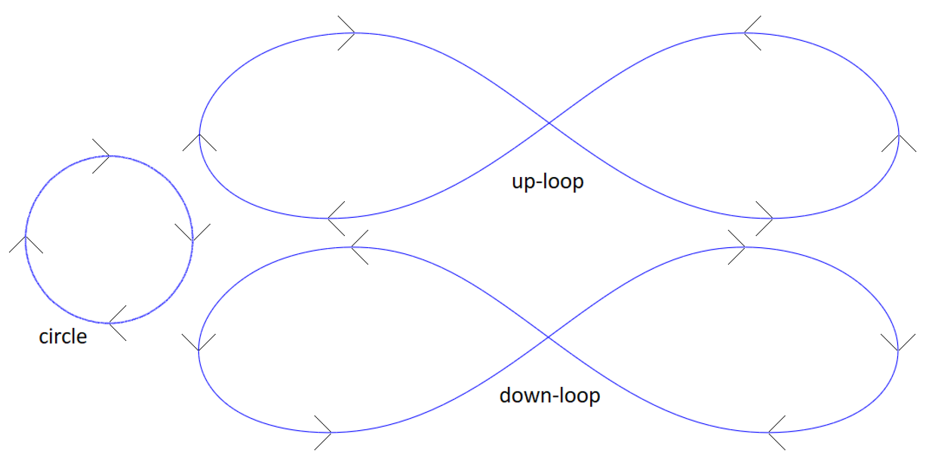
For this analysis, the aircraft fly figure-eight up-loops (Figure 1), rather than circles or figure-eight down-loops. Down loops provide the most consistent power throughout a cycle, but down loops (and circles) require flying directly downward, which is the worst case for robustness to gusts. Circles additionally require a tether unwinder, involving additional hardware and complexity.

The path is defined by tether angles, such that it scales automatically with tether length. The horizontal and vertical extents as well as the mean vertical location are modified by the trajectory optimizer. Other path Fourier coefficients affect the shape of the figure-eight. The initial path used is a figure-eight which maximizes the minimum turn radius.

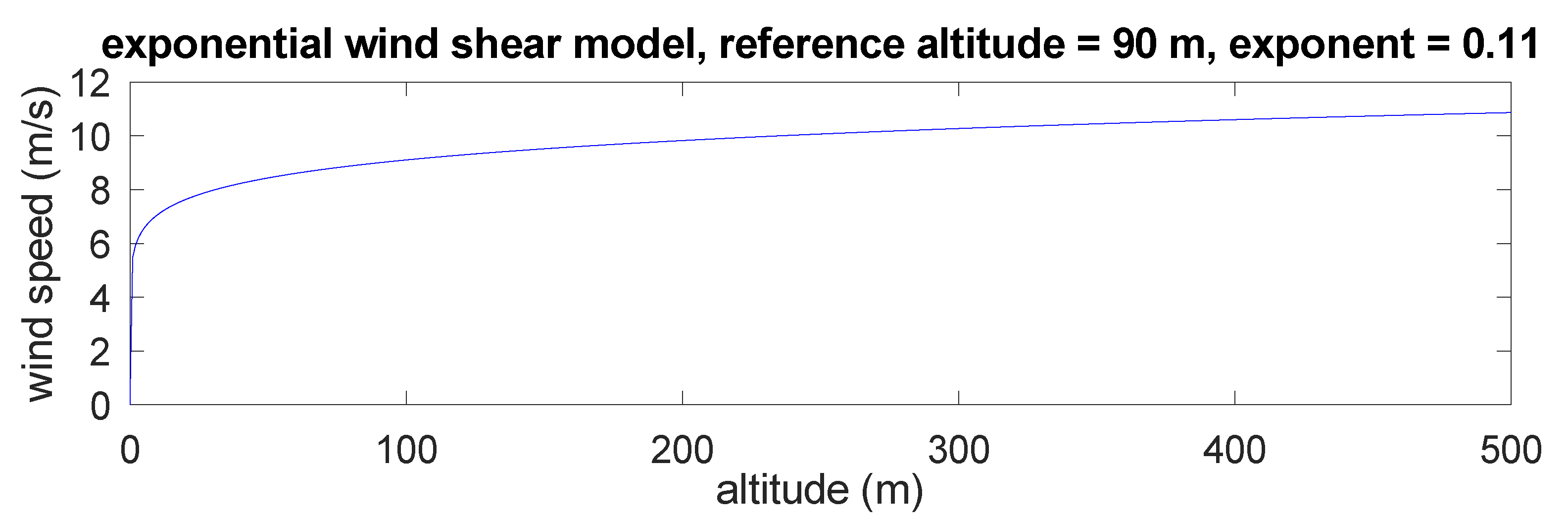
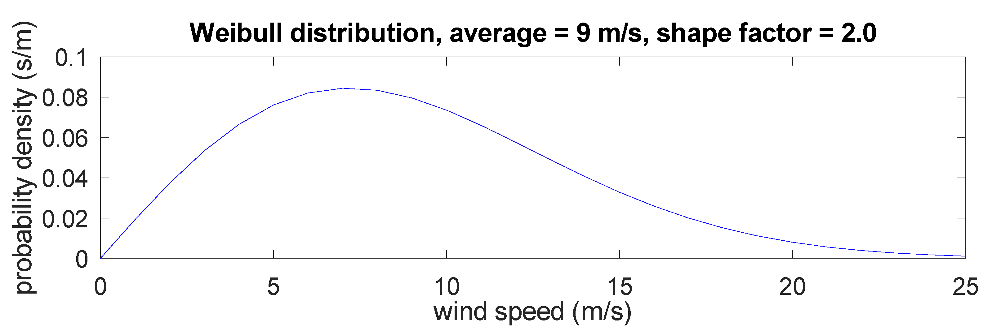
Wind speed with altitude is modeled as a power law wind profile, which involves the speed ($V_{w,0}$) at a reference altitude ($z_0$), and a shear exponent ($V_{w,exp}$), such that $V_w=V_{w,0}{(z/z_0)}^{V_{w,exp}}$. The wind shear exponent used is $0.11$, which is reasonable for offshore environments, and the reference altitude is 90 m, comparable to existing traditional offshore wind systems (see Figure 2). This neglects phenomena such as low-level jets which may have significant effects on power production in some locations. The wind is assumed to have a probability density function given by a Weibull distribution with an average of 9 m/s and a shape factor of $2.0$ (Figure 3).

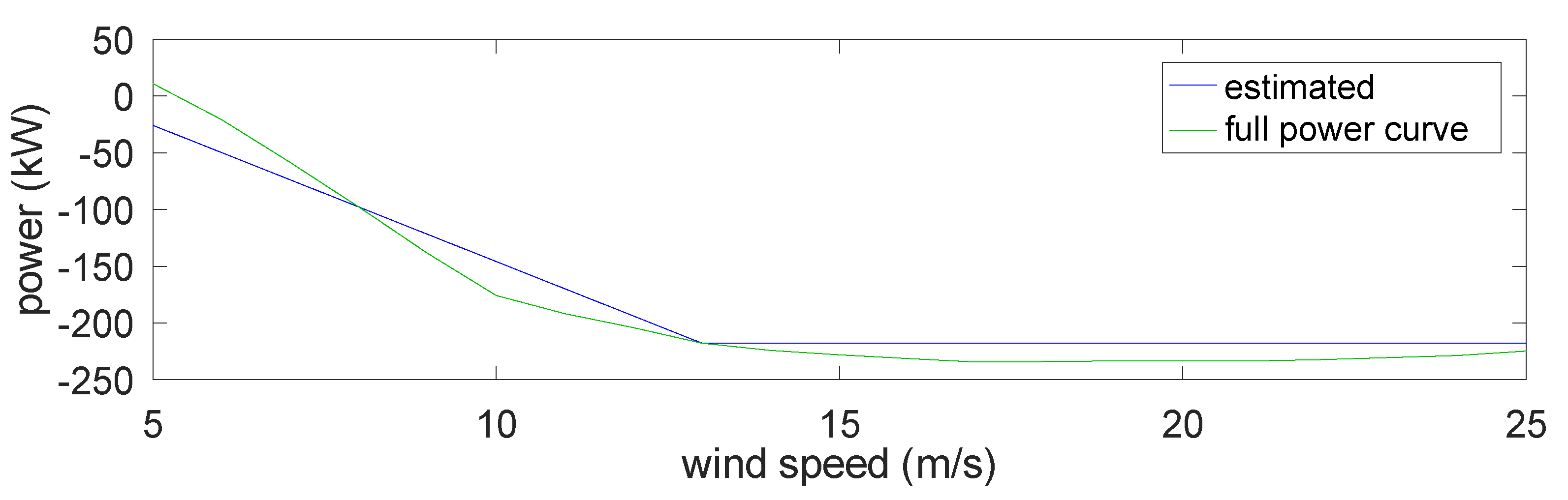
Power vs. wind speed is cubic for unconstrained wind energy systems, however tension and power constraints cause the power curve to taper off and reach a maximum at the rated wind speed [8]. In practice, fitting power curves with a linear approximation up to the rated speed and a constant above the rated speed produces a good estimate with reduced computation. For this analysis, a nominal wind speed of 13 m/s is used as the rated speed, which is comparable to traditional offshore wind systems. Power curves are estimated by optimizing trajectories at two points, 8 m/s and 13 m/s, and assuming a trapezoidal power curve which is linear up to 13 m/s and constant from 13 m/s to a cut-out speed at 25 m/s. The extrapolation below 8 m/s is used to find the cut-in speed. For the final iteration of each optimization, full power curves are evaluated at each integer wind speed between 5 m/s and 25 m/s in order to validate the use of the trapezoidal power curve estimates for the optimization. The cut-in speed is typically between 5 m/s and 7 m/s, and speeds above 25 m/s only occur approximately $0.23\%$ of the time given the assumed wind profile, so it is assumed that speeds outside this range can be neglected.

The maximum airspeed ($V_{a,max}$) is constrained such that a $20\%$ higher airspeed at the stalled lift coefficient produces a lift of $T_{max}$ (see Equation (19)). The initial maximum airspeed in 42 m/s and the minimum airspeed (below which attitude control may become unreliable) is 20 m/s.

Aspect Ratio and Reynold’s Number Effects

Airfoils can be designed to have higher maximum $C_L$ at higher Reynold’s numbers, however this relationship is not well defined. For this analysis, it is assumed that an airfoil can be designed with a maximum lift given by Equation (13) for $Re\ge 350$ k. Reynold’s number increases with increasing wing area and decreases with increasing aspect ratio (Equation (14)).

$$\begin{array}{cc}\hfill C_{L,max}=& 2.5+6E-7Re\hfill \end{array}$$

(13)

$$\begin{array}{cc}\hfill Re=& \frac{V_a{c}_w}{\nu }=\frac{V_a\sqrt{A_w}}{\nu \sqrt{AR}}\hfill \end{array}$$

(14)

Induced drag (Equation (16)) is inversely proportional to aspect ratio and is a major component of system drag (Equation (15)), especially at high lift coefficients. Induced drag increases with $C_L^2$, therefore $C_L^3/C_{D,sys}^2$ approaches zero as $C_L$ becomes very large. This parameter is also equal to zero at $C_L=0$, so there is an optimal $C_L$ (Equation (17)) and maximum $C_L^3/C_{D,sys}^2$ (Equation (18)) for a system. Because $C_{D,teth}\propto \lambda \propto \sqrt{AR}$ (Equation (43)), the benefit of increasing aspect ratio on system performance appears slightly larger than the benefit of decreasing aspect ratio on packing units more closely (from Equation (12)).

$$\begin{array}{cc}\hfill C_{D,sys}=& C_{D,i}+C_{D,p}+C_{D,teth}\hfill \end{array}$$

(15)

$$\begin{array}{cc}\hfill C_{D,i}=& \frac{C_L^2}{\pi ARosw}\hfill \end{array}$$

(16)

$$\begin{array}{cc}\hfill C_{L,opt}=& \sqrt{(}3\pi ARosw(C_{D,p}+C_{D,teth}))\hfill \end{array}$$

(17)

$$\begin{array}{cc}\hfill C_L^3/C_{D,sys}^2\le & \frac{{(3\pi ARosw)}^{3/2}}{16\sqrt{(}{C}_{D,p}+C_{D,teth})}\hfill \end{array}$$

(18)

However, this neglects the effect of mass, the coupling between tether diameter and power, and assumes that $C_{L,max}\ge C_{L,opt}$. Therefore aspect ratio is an independently varied parameter in this analysis.

This analysis assumes constant, parasitic drag ($C_{D,p}=0.04$) and Oswald Efficiency ($osw=0.71$). Tether drag normalized to wing area, $C_{D,teth}$, is typically around 0.15, resulting in $C_{L,opt}\approx 4.5$. Because this is larger than $C_{L,max}$ for Reynold’s Numbers in the range studied, higher lift always increases $C_L^3/C_{D,sys}^2$.

2.4. Aircraft Mass Scaling

Mass is normally expected to scale with length cubed. For aerodynamic applications, loads increase with length squared while distances increase with length, therefore structural masses increase with length cubed. This relationship, which can be expressed as $m\propto L^3$, $m\propto A^{3/2}$, or $m/A\propto m^{1/3}$, is a close fit for data on both manufactured aircraft and flying animals [27].

Though the mass of an aircraft is expected to increase with $A_w^{3/2}$, by changing elements like the bridle (and therefore the load distribution on the structure) or the number of rotors with scale, it is possible that AWE aircraft mass may scale with area to a lower exponent. To capture this uncertainty in the mass of a scaled system, optimizations are performed on heavier and lighter systems at each scale. For this analysis, the reference design is a 60 kg, 4 m${}^2$, 16 aspect ratio aircraft. The lightweight scaled systems assume constant mass/area with a scaled reference mass ($m_{UAV,ref}$) of 15 kg/m${}^2{A}_w$, and the heavier systems assume mass is proportional to length cubed with a scaled reference mass of 7.5 kg/m${}^3{A}_w^{3/2}$. The maximum electrical power of each scaled reference design ($P_{ref}$, Equation (20)) assumes a rated wind speed ($V_{w,rated}=13$ m/s) and a reference tether drag ($C_{D,teth,ref}=0.15$). The maximum tension of each scaled reference design ($T_{ref}$, Equation (19)) assumes the lift coefficient at stall at a maximum air speed of 42 m/s, with a $20\%$ safety factor on airspeed. The reference tether length is $20b_w$ (${\lambda }_{b,ref}=20$). The tether voltage ($V_{teth}$) is $800\sqrt{(}{A}_w)$ and does not change with the optimization. These values are summarized in

Table 1. Scaled reference design parameters.

${\mathit{A}}_{\mathit{w}}$ (m${}^2)$	4	9	16	25	36
$C_{L,max}$	2.911	3.116	3.322	3.527	3.733
$P_{ref}$ (kW)	42.0	99.3	183.3	294.5	432.9
$T_{ref}$ (kN)	18.1	43.6	82.7	137.2	209.1
lighter $m_{UAV,ref}$ (kg)	60	135	240	375	540
heavier $m_{UAV,ref}$ (kg)	60	202.5	480	937.5	1620
$\lambda$ (m)	160	240	320	400	480
$V_{teth}$ (V)	1600	2400	3200	4000	4800

.

$$\begin{array}{cc}\hfill T_{ref}=& 0.5\rho {(1.2V_{a,max})}^2{C}_{L,max}{A}_w\hfill \end{array}$$

(19)

$$\begin{array}{cc}\hfill P_{ref}=& 0.5\frac{2}{27}\rho A_w{(V_{w,rated}cos({\theta }_{t0}))}^3\frac{C_{L0}^3}{{(C_{D,UAV}+C_{D,teth,ref})}^2}\hfill \end{array}$$

(20)

For each scaled reference design, the component mass is calculated according to the distribution given in

Table 2. Component mass distribution.

${\mathit{m}}_{\mathit{ref},\mathit{struct}}$	Wing + Fuselage + Tail + Actuators	50%
$m_{ref,rot}$	SFG+prop	15%
$m_{ref,mot}$	Motor	15%
$m_{ref,pow}$	Power electronics	10%
$m_{ref,RCU}$	Roll Control Unit (RCU)	10%

(i.e., $m_{ref,struct}=0.5m_{UAV,ref}$). As the design parameters change, the changes in component masses are calculated from the scaled reference design in order to compute a new aircraft mass. The following sections derive laws for how the component masses change with changes in the design parameters.

2.4.1. Structural Scaling

The moment of inertia for an I or C section ($I_{sec}$) where the cap width is $w_{cap}$ and the thickness of the caps ($t_{cap}$) is much smaller than the section height ($h_{sec}$) is approximated by Equation (21). The maximum bending stress ($\sigma$) on a beam of length L with a distributed load (F) is given by Equation (22).

$$\begin{array}{cc}\hfill I_{sec}=& \frac{w_{cap}{t}_{cap}{h}_{sec}^2}{2}\hfill \end{array}$$

(21)

$$\begin{array}{cc}\hfill \sigma =& \frac{FL{h}_{sec}}{4I_{sec}}\hfill \end{array}$$

(22)

For a wing supported in the center, the bending equation (Equation (22)) applies to half the maximum tension and half the span where the section height is the wing thickness (Equation (23)). Assuming a constant airfoil section, wing thickness ($t_w$) is proportional to chord length ($c_w$). Also assuming spar cap width is proportional to chord length, the proportionality for spar cap thickness is given by Equation (24) and the spar mass proportionality is given by Equation (25). Note that assuming $T_{max}\propto A_w$ makes the mass proportional to $b_w^3$, which is consistent with square-cube scaling. The structural mass of the wing, fuselage, and tail ($m_{struct,w}$) is modified by Equation (26) to account for changes in maximum tension and aspect ratio.

$$\begin{array}{cc}\hfill {\sigma }_w=& \frac{T_{max}{b}_w}{16w_{cap}{t}_{cap}{t}_w}\hfill \end{array}$$

(23)

$$\begin{array}{cc}\hfill t_{cap}\propto & T_{max}{b}_w/c_w^2\hfill \end{array}$$

(24)

$$\begin{array}{cc}\hfill m_{struct,w}\propto & w_{cap}{t}_{cap}{b}_w\propto \frac{T_{max}{b}_w^2}{c_w}\propto T_{max}{A}_w^{1/2}A{R}^{3/2}\hfill \end{array}$$

(25)

$$\begin{array}{cc}\hfill m_{struct}=& m_{ref,struct}\frac{T_{max}}{T_{ref}}{(\frac{AR}{A{R}_{ref}})}^{3/2}\hfill \end{array}$$

(26)

2.4.2. Rotor Sizing

The maximum power output (Equation (27)) and drag (Equation (28)) of a turbine are defined by the Betz Limit [28]. This is used to calculate the total area of $n_{rot}$ rotors (Equation (29)) and radius of each rotor (Equation (30)) from the maximum power. The maximum rotor rotational speed is limited by a Mach number of 0.85 at the blade tips (Equation (31)).

$$\begin{array}{cc}\hfill P_{max}\le & \frac{8}{27}\rho A_{rot}{V}_a^3\hfill \end{array}$$

(27)

$$\begin{array}{cc}\hfill D_{rot}\le & \frac{8}{27}\rho A_{rot}{V}_a^2\hfill \end{array}$$

(28)

$$\begin{array}{cc}\hfill A_{rot}=& \frac{27P_{max}}{8\rho V_{a,max}^3}\hfill \end{array}$$

(29)

$$\begin{array}{cc}\hfill R_{rot}=& \sqrt{(}\frac{A_{rot}}{\pi n_{rot}})=\sqrt{(}\frac{27P_{max}}{8\pi n_{rot}\rho V_{a,max}^3})\hfill \end{array}$$

(30)

$$\begin{array}{cc}\hfill {\omega }_{rot}\le & \frac{0.85a}{R_{rot}}\hfill \end{array}$$

(31)

A constant efficiency of $70\%$ is used for conversion from drag power to electrical power when generating ($P_e=\eta P_m$) and from electrical power to thrust power ($P_m=\eta P_e$).

For a rotor, the bending equation (Equation (22)) applies to the rotor radius, $R_{rot}$, and the force, $D_{rot}$ (Equation (28)) divided by the number of blades on all rotors (Equation (32)). Assuming spar cap width and blade thickness are proportional to blade chord ($c_b$), the proportionality for spar cap thickness is given by Equation (33), and blade mass (Equation (34)) is consistent with square-cube scaling assuming a constant blade aspect ratio and $D_{rot}\propto R_{rot}^2$. Note that the mass of the pylon/sideforce generator supporting the rotor scales the same way because its length is approximately the rotor radius and the force it supports is the rotor force. The structural mass of the rotor blades, hubs, and pylon/sideforce generators is modified by Equation (35) to account for changes in maximum power.

$$\begin{array}{cc}\hfill {\sigma }_{rot}=& \frac{D_{rot}{R}_{rot}}{4n_{blades}{n}_{rot}{w}_{cap}{t}_{cap}{t}_b}\hfill \end{array}$$

(32)

$$\begin{array}{cc}\hfill t_{cap}\propto & D_{rot}{R}_{rot}/(n_{rot}{n}_{blades}{c}_b^2)\hfill \end{array}$$

(33)

$$\begin{array}{cc}\hfill m_{blades}\propto & n_{rot}{n}_{blades}{R}_{rot}{c}_b{t}_{cap}\propto \frac{D_{rot}{R}_{rot}^2}{c_b}\hfill \end{array}$$

(34)

$$\begin{array}{cc}\hfill m_{rot}=& m_{ref,rot}{(\frac{P_{max}}{P_{ref}})}^{3/2}\hfill \end{array}$$

(35)

2.4.3. Electrical Scaling

It is assumed that tether voltage scales with length (Equation (36), see Section 2.4.5), and that the mass ($m_{pow}$) and volume of any power electronics scale proportionally with maximum power (Equation (37)), which is equivalent to scaling with current at a constant wing size/voltage.

$$\begin{array}{cc}\hfill V_{teth}=& r_v\sqrt{A_w}\hfill \end{array}$$

(36)

$$\begin{array}{cc}\hfill m_{pow}=& m_{ref,pow}\frac{P_{max}}{P_{ref}}\hfill \end{array}$$

(37)

It is assumed that motor mass ($m_{mot}$) scales with maximum motor torque ($T_{rot}$). Motor torque is generated by magnetic fields which are limited by inductor saturation, which is limited by the mass and magnetic permeability of the motor magnetic core. Maximum shaft power (Equation (38)) is related to maximum electrical power by an efficiency and maximum rotor speed is inversely proportional to radius (Equation (31)), which is proportional to $\sqrt{P_{max}}$ (Equation (27)), therefore motor torque is proportional to $P_{max}^{3/2}$ (Equation (39)). Therefore motor mass is related to maximum power by the same square-cube law (Equation (40)) as the rotor and sideforce generator (Equation (35)).

$$\begin{array}{cc}\hfill P_{shaft}=& {\omega }_{rot}{T}_{rot}=\eta P_{max}\hfill \end{array}$$

(38)

$$\begin{array}{cc}\hfill T_{rot}\propto & P_{max}{R}_{rot}\propto P_{max}^{3/2}\propto R_{rot}^3\hfill \end{array}$$

(39)

$$\begin{array}{cc}\hfill m_{mot}=& m_{ref,mot}{(\frac{P_{max}}{P_{ref}})}^{3/2}\hfill \end{array}$$

(40)

2.4.4. Roll Control Unit

The roll control unit connects to the tether and uses a motor to vary the length of the bridle lines, setting the roll angle of the aircraft relative to the tether. The RCU structure is driven by maximum tether tension, but the motor is sized by the roll moment required on the aircraft, i.e., the differential bridle line tension rather than total tension. Roll torque is approximately roll inertia times roll acceleration ($L_i\approx I_{xx}\dot{p}$). Roll rate (p) is inversely proportional to tether length ($\lambda ={\lambda }_b\sqrt{AR{A}_w}$), assuming the same roll angles are required to follow a path with the same tether angles at the same speed, because the path size increases linearly with tether length, providing linearly more time to roll. Roll acceleration ($\dot{p}$) is inversely proportional to tether length squared because of the lower roll rate and the increased time to change roll rate. Roll inertia is proportional to mass and span squared, and using the mass from Equation (26) yields Equation (41). Because this expression for the RCU motor scaling is very similar to the structural mass scaling of the aircraft, it is assumed to be reasonable for both motor and structural scaling for the RCU (Equation (42)).

$$\begin{array}{cc}\hfill L_i=& I_{xx}\dot{p}\propto \frac{m_{UAV}{b}_w^2}{{\lambda }_b^2{b}_w^2}\propto \frac{T_{max}A{R}^{3/2}}{{\lambda }_b^2}\hfill \end{array}$$

(41)

$$\begin{array}{cc}\hfill m_{RCU}=& m_{ref,RCU}\frac{T_{max}}{T_{ref}}{(\frac{AR}{A{R}_{ref}})}^{3/2}{(\frac{{\lambda }_{b,ref}}{{\lambda }_b})}^2\hfill \end{array}$$

(42)

2.4.5. Tether Design

The tether adds mass and drag to the system. The tether drag is proportional to a 2D drag coefficient ($C_{d,teth}$), diameter ($d_{teth}$), length, and $k_{dv}$ (a factor related to the difference in air velocity along the length of the tether and the fraction of tether drag reacted at the aircraft vs. at the ground, which is around $\frac{1}{4}$). The tether drag coefficient normalized by the wing area is given by Equation (43). The reference tether length is 20× the aircraft span, or $20\sqrt{A_{w}AR}$.

$$\begin{array}{cc}\hfill C_{D,teth}=& k_{dv}{C}_{d,teth}\frac{d_{teth}\lambda }{A_w}\propto \frac{d_{teth}\lambda }{A_w}\hfill \end{array}$$

(43)

The tether is made up of a strength member, conductors, insulative layers, and an outer jacket. For this paper, a tether design is performed for each vehicle, resulting in an appropriate tether drag and lift to drag ratio for the UAV-tether combined system, and a tether mass determined by the proportions of copper, strength member, insulation, and jacketing required. The cross-sectional area of the tether strength member is proportional to maximum tension (and therefore to the wing area), the insulative layer thickness is proportional to voltage, and the jacket is a constant thickness. Conductor area ($A_c$) determines tether resistance (Equation (45)), which must be low enough to maintain a reasonable voltage drop and keep heat generation below a critical value.

For systems with the same voltage maintaining the same voltage drop (Equation (44)), tether resistance must be be inversely proportional to power (Equation (45)). Because power is proportional to wing area and tether length is proportional to the square root of wing area, conductor cross-sectional area must increase with wing area to the $3/2$ power (Equation (46)). Therefore, to keep the conductor area to wing area ratio constant, system voltage must increase with the square root of tether length.

$$\begin{array}{cc}\hfill r_t=& \frac{I^2{R}_{teth}}{P_{max}}=\frac{I{R}_{teth}}{V_{teth}}=\frac{P_{max}{R}_{teth}}{V_{teth}^2}\hfill \end{array}$$

(44)

$$\begin{array}{cc}\hfill R_{teth}=& r_t\frac{V_{teth}^2}{P_{max}}=\frac{{\rho }_c\lambda }{A_c}\hfill \end{array}$$

(45)

$$\begin{array}{cc}\hfill A_c=& \frac{{\rho }_c\lambda P_{max}}{r_t{V}_{teth}^2}\propto \frac{\sqrt{AR}A{w}^{3/2}}{V_{teth}^2}\hfill \end{array}$$

(46)

Given a heat limit on the power dissipated in the tether per unit tether length ($p_{heat}$, Equation (47)), a required conductor area can be computed (Equation (48)). Because power is proportional to wing area and tether length is proportional to the square root of wing area, in order to keep the conductor area to wing area ratio constant, system voltage must increase with the tether length. Therefore tethers will usually be limited by heat dissipation rather than voltage drop, and tether voltage must scale with tether length.

$$\begin{array}{cc}\hfill p_{heat}\lambda =& I^2{R}_{teth}=\frac{P_{max}^2{\rho }_c\lambda }{V_{teth}^2{A}_c}\hfill \end{array}$$

(47)

$$\begin{array}{cc}\hfill A_c=& \frac{P_{max}^2{\rho }_c}{V_{teth}^2{p}_{heat}}\propto \frac{A{w}^2}{V_{teth}^2}\hfill \end{array}$$

(48)

Keeping the conductor area to wing area ratio constant doesn’t keep the tether drag coefficient exactly constant, but because the required insulation thickness increases linearly with voltage (and tether length), $C_{D,teth}$ for typical tethers stays within a relatively narrow range close to 0.14.

2.5. Economic Assumptions

Levelized Cost of Energy (LCOE) is used as the metric for optimization (Equation (49)), defined by annual costs (operations and maintenance for the year, $OpEx$, plus a “mortgage payment” on the initial capital costs, $CapExFCR$) divided by annual energy production ($AEP$). A recent ARPA-E FOA for floating offshore wind turbines (DE-FOA-0002051 [29]) provides a method for calculating LCOE which appears to be a rational compromise between good fidelity and practicality of implementation for conceptual systems. The ARPA-E method assumes a fixed charge rate (FCR) of $8.2\%$ and a fixed operations and maintenance cost (OpEx) of $\$86$/kW. Annual electricity production (AEP) is determined by summing the power curve for a proposed design weighted by a Weibull distribution with a shape factor of $2.1$ and a scale factor of $10.13$. The RFP determines the total capital expenditure (CapEx) of offshore wind systems with specified costs per kilogram for materials, manufacturing, and installation for each component (Equation (50)).

$$\begin{array}{cc}\hfill LCOE=& \frac{CapExFCR+OpEx}{AEP}\hfill \end{array}$$

(49)

$$\begin{array}{cc}\hfill CapEx=& \sum _{j=component}mas{s}_j(c_{t,j}+c_{m,j}+c_{i,j})\hfill \end{array}$$

(50)

This analysis adapts the ARPA-E method for AWE systems: the values for the rotor blades are applied to the AWE aircraft structure, the values for the nacelle (including generator, drive train, and yaw bearing) are applied to the motor and power electronics, the values for the tower installation and maintenance are applied to the tether while the tether material is assumed to be mostly copper rather than steel, and the floating platform, mooring, and anchor are unaffected as they exist for both traditional and airborne offshore systems. A summary of the cost values and the results for the reference design are given in

Table 3. Cost per kg values.

	${\mathit{c}}_{\mathit{t}}$ (Material $/kg)	${\mathit{c}}_{\mathit{m}}$ (Manufacture $/kg)	${\mathit{c}}_{\mathit{i}}$ (Installation $/kg)	Unit Cost $
Structure	8	30.96	0.8	2982
Generator, Inverter	2	18.98	0.2	529.5
Tether, Interconnects	3	20	0.2	1887
Floating platform	2	4	0.26	12,520
Mooring system	2	0.28	1.04	498
Anchor system	0.6	4.02	2.088	1006.2

. Masses for the floating platform, mooring, and anchor are assumed to be 20 kg/kW, $1.5$ kg/kW, and $1.5$ kg/kW, based on linear scaling with a reference design. Electrical interconnects are neglected by the ARPA-E method, but are a larger fraction of the capital expenditures for a more distributed farm, and are therefore included here. It is assumed that the interconnects do not have to be buried, therefore the interconnects use the same cost values as the tethers, which carry similar power over similar distances in similar environments. This analysis also replaces the constant OpEx value by assuming an average lifetime for the aircraft (2 years) and for the platform and underwater components (5 years) and dividing the CapEx for those components by their lifetime to obtain an average replacement cost per year.

The two-year lifetime assumes AWE development will resemble aircraft development, which shows a consistent relationship between hours flown and reliability (after a few hundred flight hours, the system mean time between failures (MTBF) should be about a week of continuous operation, after 1000 flight hours MTBF is about a month, and after 100,000 flight hours MTBF is about a year) [30]. The most mature aircraft have MTBFs equivalent to around 2 years of continuous operation. Smaller scale AWE systems will benefit from lower development costs. Flying 100,000 h on aircraft that last from 100 h to 10,000 h requires building and crashing a lot of prototypes, and a smaller scale is advantageous for this development process.

3. Design Optimization Results

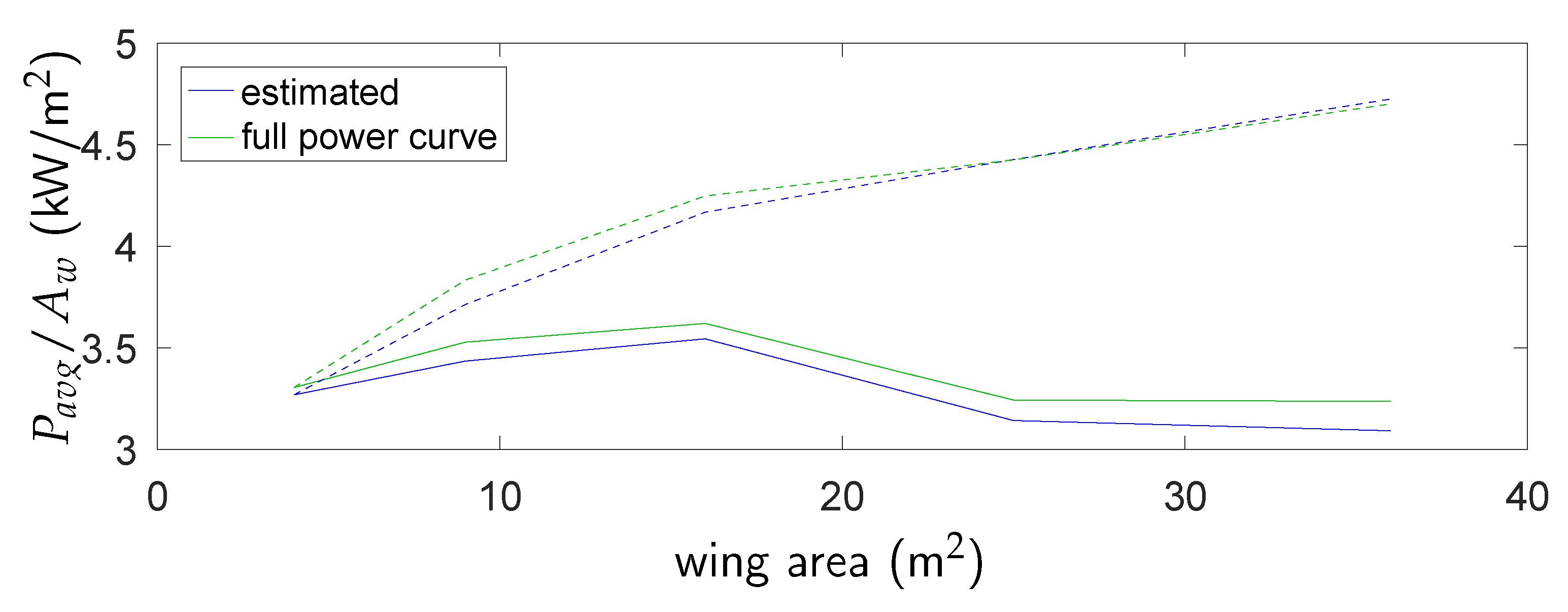
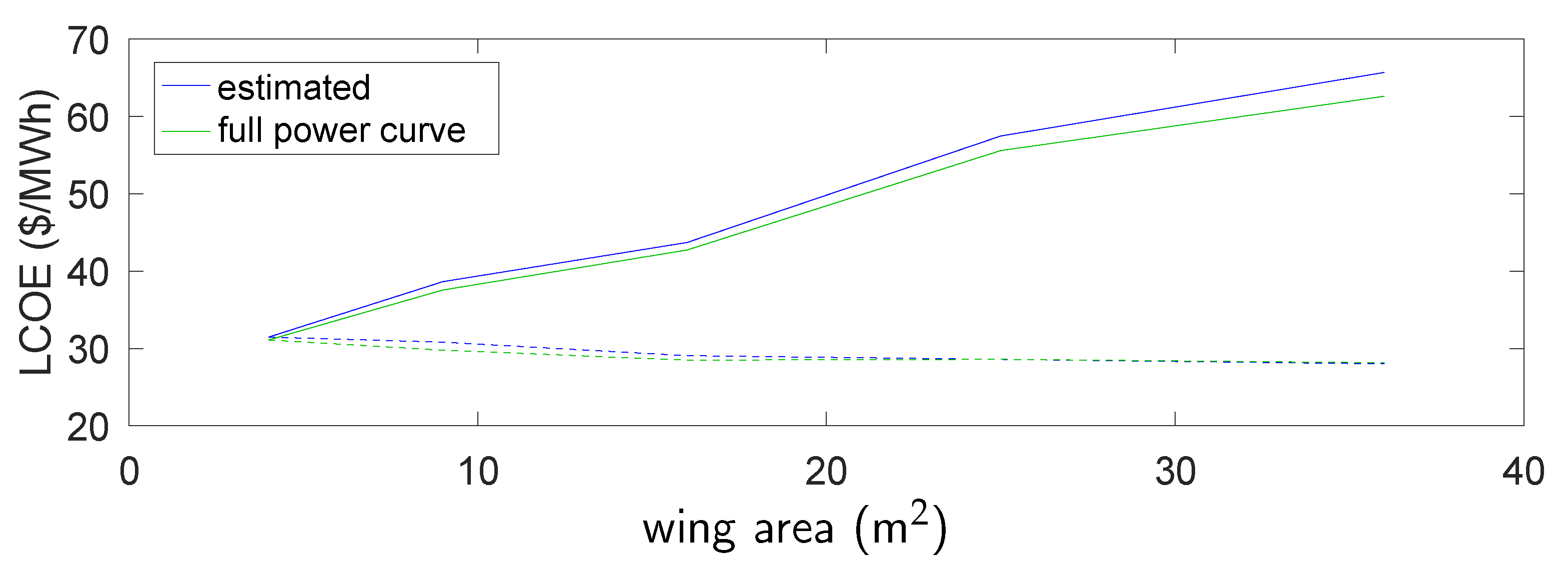
A representative power curve (Figure 4) shows that the power curve estimates (blue) match the full power curves (green) relatively well, as do the average power results (Figure 5) and the LCOE estimates (Figure 6) for the estimated (blue) and full (green) power curves.

The design parameters ($AR$, $P_{max}$, $T_{max}$, and $\lambda$), as well as selected dependent parameters, for the optimized systems are shown in

Table 4. Optimized design params.

${\mathit{A}}_{\mathit{w}}$ (m${}^2$)	4	9	9	16	16	25	25	36	36
$AR$	16	15.8	15.9	15.9	16	15.9	15.9	15.7	15.7
$P_{max}$ (kW)	44	106	106	194	192	307	308	448	449
$T_{max}$ (kN)	16.1	43.1	43.5	82.6	81.2	136	136	208	209
$\lambda$ (m)	160	240	240	319	320	398	399	473	476
$C_{L0}$	2.91	3.12	3.12	3.33	3.32	3.53	3.53	3.74	3.74
$C_{D,UAV}$	0.278	0.315	0.313	0.353	0.348	0.391	0.391	0.439	0.439
$C_{D,teth}$	0.133	0.137	0.137	0.139	0.138	0.14	0.14	0.141	0.142
$L/D$	7.09	6.9	6.92	6.77	6.83	6.66	6.64	6.46	6.45
$V_{a,max}$ (m/s)	39.6	41.7	41.9	41.9	41.6	41.8	41.8	41.9	41.9
$m_{UAV}$ (kg)	57.4	137	209	245	488	380	952	543	1630
$m_{teth}$ (kg)	16.9	66	66.4	167	164	337	340	606	611
$d_{teth}$ (mm)	11	17.1	17.2	23.1	23	29.2	29.3	35.7	35.7

. $T_{max}$ and $AR$ are regularly lower than their reference values while $P_{max}$ is regularly higher than $P_{ref}$. Tether length doesn’t change as much.

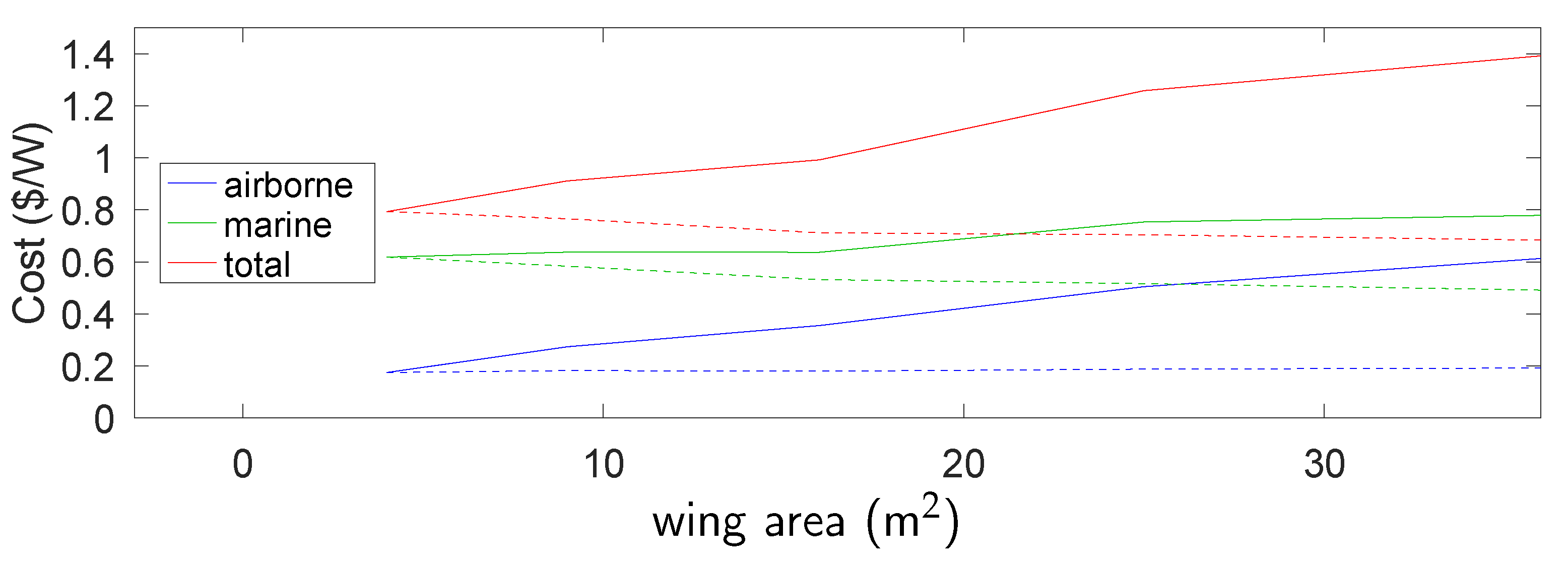
The levelized cost of energy calculated for the optimal systems is shown in Figure 6, both for the estimated and full power curves. The upper and lower curves represent the heavier (solid line) and lighter (dotted line) system assumptions, respectively. The vertical range between these curves can be thought of as the uncertainty due to uncertainty in mass scaling. The contributors to LCOE, namely average power and system cost, are shown in Figure 5 and Figure 7, respectively. Note that for Figure 5, the upper curve represents the lighter systems (dotted line). For Figure 7, “airborne” includes the aircraft structure, electronics, and tether while “marine” includes the floating platform, mooring, anchors, and electrical interconnects. Again, dotted lines represent the light systems, and solid lines represent the heavy systems.

4. Discussion

As noted in the results, values computed from a power curve extrapolated from two points closely matches a full power curve, which validates the two-point method and provides confidence that optimizations performed using the estimated power curve are real optimums.

Based on the design parameters following optimization, it appears that the reference design was underpowered and structurally overbuilt, and the optimizations corrected that for each scaled reference design. The tether length doesn’t change as much, indicating that either the reference tether length is close to the optimal tether length or LCOE is not very sensitive to tether length near the reference value. Because the slope of LCOE vs. tether length is zero at the optimum, both are likely true.

LCOE values from different studies can’t necessarily be compared directly (cost estimates for existing technologies can be substantially different between sources such as [3,4]). This study is more difficult to compare because it estimates costs at a future development stage where AWE aircraft have a 2-year MTBF and floating systems have a 5-year MTBF (systems with longer lifetimes would be substantially cheaper and less reliable systems more costly). However, ignoring the details (such as the learning rate for competing technologies or different interest rates for projects with different perceived risks or different water depths available to different technologies, etc.) and assuming these results can be directly compared to s $92/MWh value for offshore wind [3], the heavy 36 m${}^2$ system would only be competitive with traditional offshore wind when fairly mature. The smaller and lighter systems would become competitive earlier (while less technologically mature and reliable).

The main takeaway is that there is a small economic benefit to scaling up AWE systems if they can be scaled at a constant weight/area, otherwise it is very advantageous to build a larger number of smaller units. The optimal size is likely to be close to wherever the lowest mass per unit area can be achieved; this is unlikely to be smaller than 4 m${}^2$ because for systems below a certain size, requirements other than operational loads (such as handling or manufacturability requirements) will drive mass. Further research, including more detailed design work to reduce uncertainty in mass, is necessary to determine the optimal scale more precisely. Further research will also involve use of a Monte Carlo method, genetic algorithm, or other method to determine if local minima are an issue for this optimization.

5. Conclusions

Airborne Wind Energy systems are lighter, easier to install, and potentially lower in cost than comparable conventional horizontal axis wind turbines but are at a lower technology readiness level. Though future work is necessary to further develop AWE designs at different scales and reduce uncertainty around the optimal scale, the physics and economics of AWE systems are very different from horizontal axis wind turbines which benefit from being as large as possible, and it appears that optimized AWE designs will involve farms with significantly smaller individual units than traditional wind farms.

References

- CAISO. What the Duck Curve Tells Us about Managing a Green Grid; Technical Report; California Independent Systems Operator: Folsom, CA, USA, 2016; Available online: www.caiso.com/Documents/FlexibleResourcesHelpRenewables_FastFacts.pdf (accessed on 15 June 2020).
- Musial, W. Offshore Wind Energy Briefing; Technical Report; California Energy Commission Integrated Energy Policy Workshop Offshore Renewable Energy: Sacramento, CA, USA, 2016. Available online: efiling.energy.ca.gov/GetDocument.aspx?tn=211749 (accessed on 15 June 2020).
- Lazard’s Levelized Cost of Energy Analysis Version 12.0. Available online: www.lazard.com/media/450784/lazards-levelized-cost-of-energy-version-120-vfinal.pdf (accessed on 15 June 2020).
- Ilas, A.; Ralon, P.; Rodriguez, A.; Taylor, M. Renewable Power Generation Costs in 2017; International Renewable Energy Agency: Abu Dhabi, UAE, 2018; Available online: www.irena.org/-/media/Files/IRENA/Agency/Publication/2018/Jan/IRENA_2017_Power_Costs_2018_summary.pdf (accessed on 15 June 2020).
- De Vries, E. Floating Offshore Takes to the Skies. Available online: www.windpowermonthly.com/article/1466082/floating-offshore-takes-skies (accessed on 15 June 2020).
- Mahbub, A.; Rehman, S.; Meyer, J.; Al-Hadhrami, L. Wind Speed and Power Characteristics at Different Heights for a Wind Data Collection Tower in Saudi Arabia. In World Renewable Energy Congress; Linköping University Electronic Press: Linköping, Sweden, 2011. [Google Scholar] [CrossRef]
- Loyd, M. Crosswind Kite Power. AIAA J. Energy 1980, 4, 106–111. [Google Scholar] [CrossRef]
- Vander Lind, D. Analysis and Flight Test Validation of High Performance Airborne Wind Turbines. In Airborne Wind Energy; Ahrens, U., Diehl, M., Schmehl, R., Eds.; Springer: Berlin/Heidelberg, Germany, 2013; pp. 473–490. [Google Scholar] [CrossRef]
- SkySails GmbH. SkySails Product Brochure. Available online: www.skysails.info/fileadmin/userupload/Downloads/ENSkySailsProductBrochure.pdf (accessed on 15 June 2020).
- Sieberling, S. Flight Guidance and Control of a Tethered Glider in an Airborne Wind Energy Application. In Advances in Aerospace Guidance, Navigation and Control; Chu, Q., Mulder, B., Choukroun, D., van Kampen, E.J., de Visser, C., Looye, G., Eds.; Springer: Berlin/Heidelberg, Germany, 2013. [Google Scholar] [CrossRef]
- Canale, M.; Fagiano, L.; Milanese, M. Power Kites for Wind Energy Generation; Fast Predictive Control of Tethered Airfoils. IEEE Control Syst. Mag. 2007, 27, 25–38. [Google Scholar] [CrossRef]
- Gros, S.; Zanon, M.; Diehl, M. Control of Airborne Wind Energy Systems Based on Nonlinear Model Predictive Control and Moving Horizon Estimation. In Proceedings of the European Control Conference, Urich, Switzerland, 17–19 July 2013. [Google Scholar] [CrossRef]
- Houska, B.; Diehl, M. Optimal Control for Power Generating Kites. In Proceedings of the 2007 European Control Conference (ECC), Kos, Greece, 2–5 July 2007; pp. 3560–3567. [Google Scholar] [CrossRef]
- Williams, P.; Lansdorp, B.; Ockels, W. Optimal Crosswind Towing and Power Generation with Tethered Kites. J. Guid. Control. Dyn. 2008, 31, 81–93. [Google Scholar] [CrossRef]
- Furey, A.; Harvey, I. Robust adaptive control for kite wind energy using evolutionary robotics. In Proceedings of the Biological Approaches for Engineering Conference, Southampton, UK, 17–19 March 2008. [Google Scholar]
- Faggiani, P.; Schmehl, R. Design and Economics of a Pumping Kite Wind Park. In Airborne Wind Energy; Springer: Singapore, 2018; pp. 391–411. [Google Scholar] [CrossRef] [Green Version]
- Frost, C.; Logan, A.; Gow, G.; Ainsworth, D. Global Prospects for Airborne Wind Onshore. In Proceedings of the Airborne Wind Energy Conference, Glasgow, UK, 15–16 October 2019. [Google Scholar]
- Zywietz, D. What will it take for Airborne Wind Energy (AWE) to be successful in Remote & Mini-grid Applications? In Proceedings of the Airborne Wind Energy Conference, Glasgow, UK, 15–16 October 2019. [Google Scholar]
- Yang, H.; Chen, J.; Pang, X. Wind Turbine Optimization for Minimum Cost of Energy in Low Wind Speed Areas Considering Blade Length and Hub Height. Appl. Sci. 2018, 8, 1202. [Google Scholar] [CrossRef] [Green Version]
- Luo, L.; Zhang, X.; Song, D.; Tang, W.; Yang, J.; Li, L.; Tian, X.; Wen, W. Optimal Design of Rated Wind Speed and Rotor Radius to Minimizing the Cost of Energy for Offshore Wind Turbines. Energies 2018, 11, 2728. [Google Scholar] [CrossRef] [Green Version]
- Wu, J.; Wang, T.; Wang, L.; Zhao, N. Impact of Economic Indicators on the Integrated Design of Wind Turbine Systems. Appl. Sci. 2018, 8, 1668. [Google Scholar] [CrossRef] [Green Version]
- Felker, F. From Kiteboard to Energy Kite: Makani’s Path to Power Generation Through Prototypes. 2017. Available online: medium.com/makani-blog/from-kiteboard-to-energy-kite-f0ced0680ed8 (accessed on 15 June 2020).
- Felker, F. A Long and Windy Road. 2020. Available online: medium.com/makani-blog/a-long-and-windy-road-3d83b9b78328 (accessed on 15 June 2020).
- Staff. Long Duration Test Flight 2018; Kitemill: Voss, Norway, 2018; Available online: www.kitemill.com/article/63/Longdurationtestflight2018 (accessed on 15 June 2020).
- Staff. Soaring High with Kite-Wind Test Flight. 2019. Available online: www.windpowermonthly.com/article/1594531/soaring-high-kite-wind-test-flight (accessed on 15 June 2020).
- Aull, M. A Non-linear Inverse Model for Airborne Wind Energy System Analysis. Wind Energy 2019, in press. [Google Scholar]
- Noth, A.; Siegwart, R. Design of Solar Powered Airplanes for Continuous Flight; Technical Report; Swiss Federal Institute of Technology: Zürich, Switzerland, 2006. [Google Scholar] [CrossRef]
- Betz, A. Introduction to the Theory of Flow Machines; Pergamon Press: Oxford, UK, 1966. [Google Scholar] [CrossRef]
- ATLANTIS Metric Space Workbook for DE-FOA-0002051; Technical Report; Advanced Research Projects Agency-Energy: Washington, DC, USA, 2019. Available online: arpa-e-foa.energy.gov/FileContent.aspx?FileID=46f075c8-cb95-4ce9-82ca-6750fce2cca9 (accessed on 1 March 2019).
- Safety Statistics of UAS in USAF. AUVSI News. 2014; Available online: www.auvsi.org/safety-statistics-uas-usaf (accessed on 15 June 2020).
Figure 1.
Closed trajectory types.
Figure 2.
Exponential wind speed model.
Figure 3.
Weibull wind speed probability density function.
Figure 4.
Power curve for light 25 m.
Figure 5.
Average power per unit wing area.
Figure 6.
Levelized Cost of Energy vs. System size.
Figure 7.
Cost per watt vs. wing area.