Sliding Mode Control with Application to Fault-Tolerant Control: Assessment and Open Problems

Abstract

This paper is prepared within a collaboration between the Instituto Politécnico Nacional, which is a Mexican research institute that manages research on sliding-mode control theory, and the ARIA research team of the Intégration du Matériau au Système Lab., a French research group that engages research on model-based fault diagnosis and fault-tolerant control theories. The paper reviews the application of sliding mode control techniques to fault tolerant control and provides perspectives leading to posing some open problems. Operating principles, definitions of the basic concepts are recalled along with the control objectives and design procedures. The evolution of the sliding mode control technique through five generations (as classified by Fridman, Moreno and co-workers) is reviewed. Their respective design procedures, limitations, and robustness properties are also highlighted. The application of the five generations of sliding-mode controllers to fault-tolerant control is discussed. The focus is on some open problems that are judged to commonly be overlooked. Some applications in real-world systems are also presented.

1. Context and Motivation

Control tasks and related methodologies have been of growing interest since the dawn of the 19th century, with the emergence of industrial production systems. These tasks are generally carried out using a device that collects, centralizes, and processes all available relevant information through sensors and acquisition chains, in order to specify control actions to be applied to the system. As of December 2020, there are no less than 406,257 publications in the Scopus scientific database and 2,060,000,000 results on the Google search engine that match the search phrase “control engineering”. Among the different approaches published in the literature, adaptive control accounts for half; i.e., it is possible to find 234,911 papers in Scopus. With the need to develop more and more intelligent and reliable solutions for autonomous systems, it is proposed in this study to focus on the categories of Sliding Mode Control (SMC) (with 42,062 papers in Scopus) and Fault-Tolerant Control (FTC) solutions (with 19,081 works in Scopus).

Some recent papers [1,2,3,4] provide good surveys of previously reported FTC solutions. Key ingredients about the design principles, as well as advantages and limitations of FTC solutions, are also reviewed, including those based on SMC approaches (see especially the very recent review [5]).

The goal of this paper is not to provide another review on FTC solutions. We invite the interested reader to refer to the works in [1,2,3,4] for such reviews. Rather, the aim of the paper is to present a critical review and perspectives leading to some problems using SMC techniques for FTC, which are often ignored by many authors. These open problems relate to:

(i)

the commonly invoked assumption of about the continuity of the fault profile that breaks the sliding motion;

(ii)

the proof of stability when an anti-windup strategy is embedded in the SMC architecture (when such a unit is considered, which is rarely the case); and

(iii)

the non-existence of a separation principle when using a fault estimator to schedule the control law, which is the most encountered solution to ensure fault tolerance with SMC techniques, as shown below.

These open issues motivated the authors to prepare this paper. The paper aims to demonstrate how SMC theory can be used to solve FTC problems. It is also shown that, even if it seems that SMC theories can be used with a little extra effort to solve FTC problems, the aforementioned open problems remain.

To proceed, the classification proposed by Fridman, Moreno, and co-workers of sliding-mode control designs into five generations, from the initial one, i.e., the first-order sliding-mode controllers, to the most recent, the fifth generation that consists of (continuous) arbitrary-order sliding-mode controllers, serves as a basis of our approach [6,7,8]. The goal is to demonstrate how these five generations of sliding mode control techniques can be used to solve FTC problems and introduce, with systematic mathematical justification, the three aforementioned open problems.

To this end, the remainder of the paper proceeds as follows In Section 2, the genesis of sliding mode control theory is recalled. Section 3 presents the principles of SMC theory and Section 4 discusses the five generations of SMC techniques. Section 5 finally discusses the application of SMC techniques to FTC problems.

Notation:$\mathbb{R}$ and ${\mathbb{R}}^{+}:=[0,\infty )\subset \mathbb{R}$ are the set of real numbers and the set of nonnegative real numbers, respectively. ${\mathbb{R}}^n$ is n-dimensional real space and ${\mathbb{R}}^{n\times m}$ is the set of real $n\times m$ matrices. $\mathbb{I}$ denotes the identity matrix of appropriate dimensions and ${\mathbb{I}}_n$ is the identity matrix of dimension n. $\left|x\right|$ represents the absolute value of x. If x is a vector in ${\mathbb{R}}^n$, $\left|x\right|$ refers the element-by-element operation, i.e., $\left|x\right|={\left[\begin{array}{c}|x_1|\dots |x_n|\end{array}\right]}^T$. $\parallel x\parallel$ refers to the Euclidean norm or the induced spectral norm. $sign\left(x\right)$ is the sign function of x. If x is a vector in ${\mathbb{R}}^n$, then $sign\left(x\right)$ refers the corresponding element-by-element operation, i.e., $sign\left(x\right)={\left[\begin{array}{c}sign\left(x_1\right)\dots sign\left(x_n\right)\end{array}\right]}^T$.

2. The Genesis of Sliding Mode Control Theory

Variable Structure Control (VSC) is a control technique proposed in 1960s by Emelyanov in the Soviet Union [9,10]. It became known outside Russia through the publications of Utkin [11,12]. Its operating principle is based on a set of feedback control rules and a decision rule, which is termed the “switching function” of the control signal. The feedback control rules and the switching function are designed to drive and then maintain the system behavior in a neighborhood of set (surface) determined by the switching condition. Therefore, the performance of the system and the behavior of the closed-loop system are modified through design of the switching function.

Following Emelyanov [10] and Utkin [12], VSC properties can be readily illustrated through a linear second-order system

$$\begin{array}{cc}\hfill & {\dot{x}}_1=x_2\hfill \\ \hfill & {\dot{x}}_2=a{x}_1+b{x}_2+u\hfill \\ \hfill & y=x_2\hfill \end{array}$$

(1)

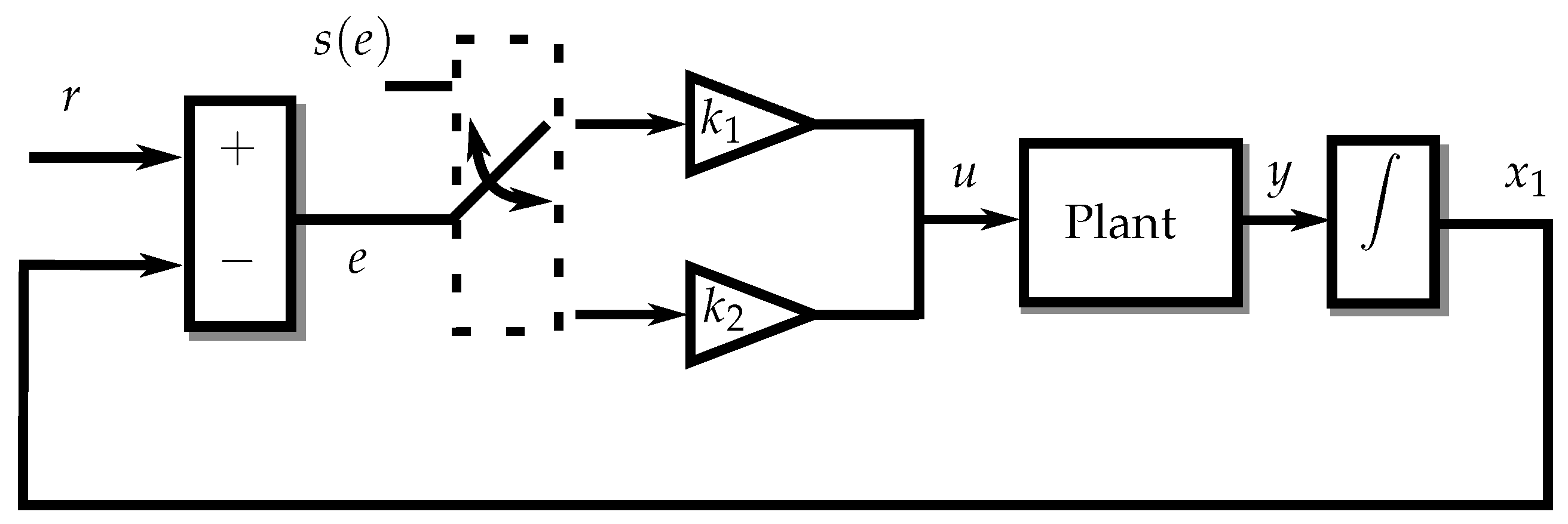
where $x_1,x_2$ are the states, u is the control signal, y is the measured output, and a and b are parameters. The main concept of VSC is illustrated in Figure 1. In Figure 1, r refers to the reference signal and $k_1,k_2$ are gains. e is the tracking error and $s\left(e\right)$ is the (error-dependent) switching condition function. Note that, nowadays, VSC has been extended to different types of systems such as discrete-time and MIMO.

Consider the control input

$$u=-\gamma x_1$$

(2)

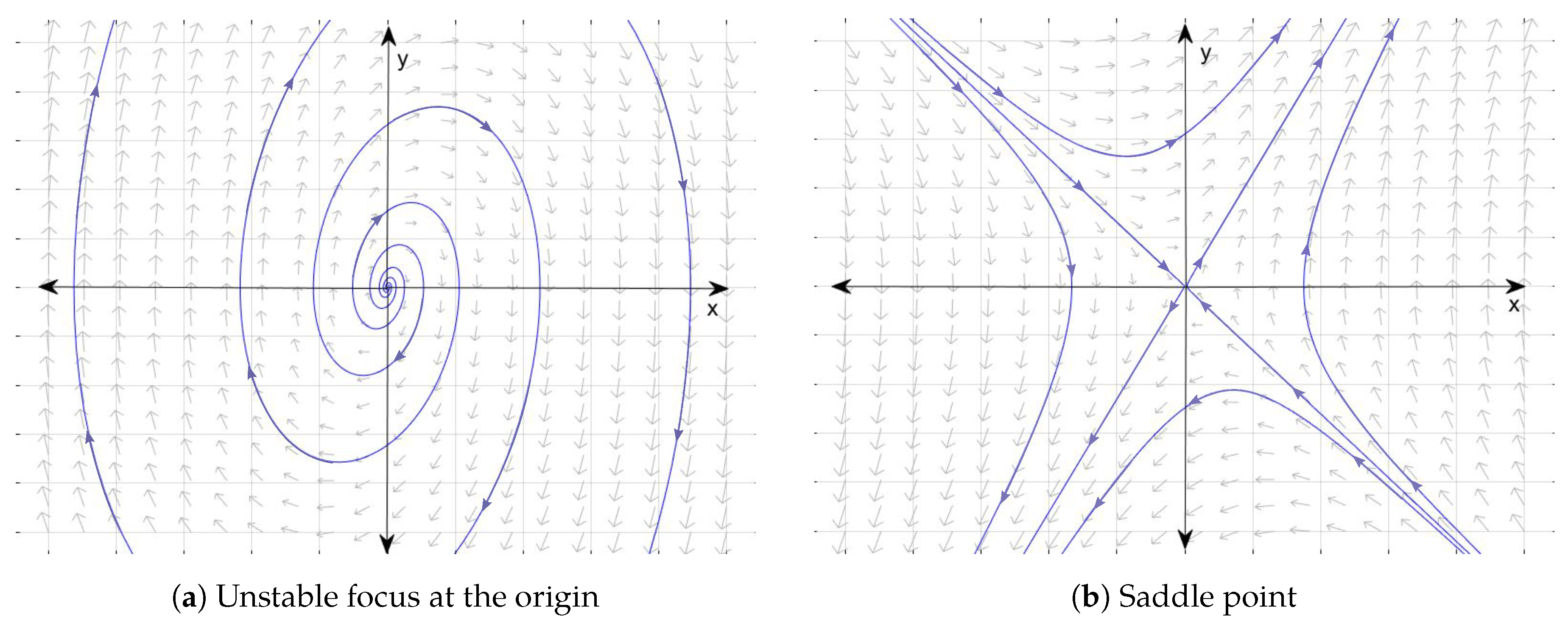
where $\gamma$ is a variable that can take values between $k_1$ and $k_2$. Suppose that, when $\gamma$ is $k_1$, the transition matrix of the closed-loop associated to Equations (1) and (2) has complex eigenvalues with positive real part. In addition, when $\gamma$ is $k_2$, the transition matrix of the closed-loop has real positive and negative eigenvalues. The behavior of the system for each case is analyzed and the result shown in terms of the phase plane in Figure 2. In Figure 2a, the behavior of system (1), with $k_1$, is shown as an unstable focus at the origin. The saddle point observed in Figure 2b belongs to the systems response when $\gamma$ is $k_2$.

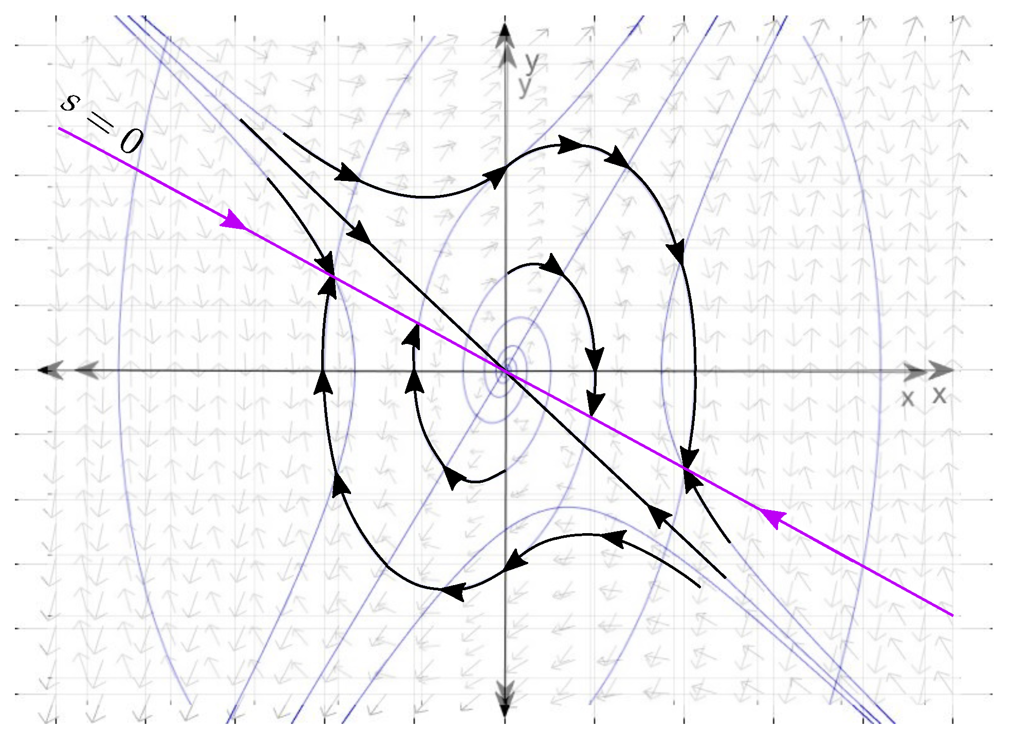
Although Figure 2 shows that both cases result in unstable systems, it can be seen that there are some regions of stability. For example, in Figure 2, for Case (b), the saddle point approaches the origin. To have the desired regions from both cases, a switching function is defined as:

$$s=s\left(x\right)=c{x}_1+x_2,c>0$$

(3)

When the switching function is equal to zero, this equation gives $s\left(x\right)=0$. Then, $\gamma$ changes its value according to the following expression:

$$\gamma =\left\{\begin{array}{cc}{k}_1,\hfill & \mathrm{when}s\left(x\right)>0\hfill \\ k_2,\hfill & \mathrm{when}s\left(x\right)<0\hfill \end{array}\right.$$

(4)

As shown in (4), the structure of the control signal (2) is changed depending on the distance of the state trajectories to the equilibrium point (the origin of the phase plane in this case). From its initial conditions, the state trajectories move firstly towards the surface characterized by $s=0$. Then, they slide to the equilibrium point along this surface. If the states move away from the sliding surface, the controller changes its structure in order to make them come back to it. In other words, high switching between control structures is involved. When the state trajectories are sliding, the value of s is theoretically equal to zero. Furthermore, when at the equilibrium point, $s=0$. These concepts are illustrated in Figure 3, where the resulting phase plane of the system under VSC is shown.

In the literature, a common variable structure for the control signal u is taken as:

$$u=\left\{\begin{array}{cc}-1,\hfill & \mathrm{when}s\left(x\right)>0\hfill \\ 1,\hfill & \mathrm{when}s\left(x\right)<0\hfill \end{array}\right.$$

(5)

where s is defined as in (3). Equation (5) can rewritten as:

$$u=-\mathrm{sign}\left(s\right(x\left)\right)$$

(6)

This variable structure control is now called Sliding Mode Control (SMC), highlighting the importance of the sliding-mode phase. The motion towards the surface $s=0$ is now called the reaching phase, and the sliding motion towards the equilibrium point along this surface is known as the sliding-mode phase. SMC demands the existence of an infinite switching frequency to maintain movement on the sliding-mode, i.e., to maintain $s\equiv 0$. The restriction of the switching to a high frequency, not an infinite one, causes the so-called chattering effect which is a high-frequency oscillation of the trajectories inside a bounded region around the sliding surface $s=0$.

3. The Fundamental Principle of SMC Techniques

In the sequel, for a better understanding, the description of the properties and the design procedure of SMC techniques are discussed for LTI systems. However, the reader should be aware that SMC theory has been extended to nonlinear systems; see, e.g., [13,14,15,16].

Consider the LTI system

$$\dot{x}\left(t\right)=Ax\left(t\right)+B\left[u\left(t\right)+f\left(t\right)\right]$$

(7)

where $A\in {\mathbb{R}}^{n\times n}$, $B\in {\mathbb{R}}^{n\times m}$. Assume that $\mathrm{rank}\left(B\right)=m$, $1\le m<n$ and the pair $(A,B)$ is controllable. In (7), $f\left(t\right)$ represents unknown disturbances and/or model uncertainties acting through the input channel, i.e., matched disturbances/uncertainties is assumed. A disturbance/uncertainty that does not act through the input channel is called unmatched. It is assumed that $f\left(t\right)$ is bounded, so that ${\left|\right|f\left|\right|}_{\infty }<\infty$. The main purpose is to design a control law that ensures the convergence of the states to zero (or to a reference in case of a tracking control problem) regardless of the profile of $f\left(t\right)$.

The first step in the design of the control law is to define the sliding surface $\mathbb{S}$ as

$$\mathbb{S}=\{x:s(x)=0\}$$

(8)

where the switching function $s\left(x\right)$ is a function of the state vector x. In this case, to be consistent with the example (7), a linear function is chosen, i.e., $s\left(x\right)=Sx$ where $S\in {\mathbb{R}}^{m\times n}$. To proceed, consider $f\left(t\right)=0$. An ideal sliding mode occurs when the state $x\left(t\right)$ converges to the sliding surface in finite-time $t_r$, i.e., the sliding phase begins at time $t\ge t_r$. This is mathematically expressed as:

$$s\left(t\right)=\dot{s}\left(t\right)=0\mathrm{for}\mathrm{all}t\ge t_r$$

(9)

The equation for sliding motion is then described as:

$$\dot{s}\left(t\right)=S(Ax\left(t\right)+Bu\left(t\right))=0$$

(10)

The necessary average value of the control signal to enforce an ideal sliding motion, i.e., $s\left(t\right)=\dot{s}\left(t\right)=0$, is called the equivalent control. It is obtained from (10) as:

$$u_{eq}\left(t\right)=-{\left(SB\right)}^{-1}\left(SAx\left(t\right)\right)$$

(11)

where S is chosen such that $SB$ is nonsingular under the aforementioned condition on rank$\left(B\right)$. This condition guarantees the existence of a unique equivalent control [17]. From (11), the equivalent control can be rewritten as a state feedback controller as:

$$u_{eq}\left(t\right)=-{\left(SB\right)}^{-1}\left(SAx\left(t\right)\right)=Kx\left(t\right)$$

(12)

It is worth noting that the equivalent control will not bring the state-trajectories to the sliding-motion. If (12) is applied to the system when it is already evolving in the sliding motion, it will maintain the movement on the sliding set. Moreover, in the case where $f\ne 0$, the equivalent control is not implementable. The concept of equivalent control should be thought as a tool to obtain a reduced order expression from which closed-loop stability can be analyzed. The closed-loop response is obtained from substituting (11) into (7), considering $f\left(t\right)=0$ as:

$$\dot{x}\left(t\right)=Ax\left(t\right)+B\left(-{\left(SB\right)}^{-1}\left(SAx\left(t\right)\right)\right)=\underset{P}{\underbrace{\left({\mathbb{I}}_n-B{\left(SB\right)}^{-1}S\right)}}Ax\left(t\right)$$

(13)

Then, P is a projection operator that satisfies the following conditions [18]:

$$SP=0,PB=0$$

(14)

Consider now the perturbed case, i.e., $f\left(t\right)\ne 0$. As mentioned previously, when the states reach the sliding surface, $s\left(t\right)=\dot{s}\left(t\right)=0$. To find the equation of the sliding motion, the derivative of $s\left(t\right)=Sx\left(t\right)$ is analyzed by using (7) as follows:

$$\dot{s}\left(t\right)=S\dot{x}\left(t\right)=S\left[Ax\left(t\right)+B\left(u\left(t\right)+f\left(t\right)\right)\right]$$

(15)

The expression of the equivalent control, for the perturbed case, is obtained by equating (15) to zero, which leads to

$$u_{eq}\left(t\right)=-{\left(SB\right)}^{-1}\left[SAx\left(t\right)+SBf\left(t\right)\right]$$

(16)

The idea of considering the equivalent control just as a tool is reinforced by the results obtained for the perturbed case, given that the equivalent control (Equation (16)) is dependent on the disturbance. The expression obtained when substituting (16) into (7), gives the closed-loop response defined as:

$$\begin{array}{cc}\hfill \dot{x}\left(t\right)& =Ax\left(t\right)+B\left[-{\left(SB\right)}^{-1}\left(SAx\left(t\right)+SBf\left(t\right)\right)\right]+Bf\left(t\right)\hfill \\ \hfill & =Ax\left(t\right)-B{\left(SB\right)}^{-1}Ax\left(t\right)-B{\left(SB\right)}^{-1}SBf\left(t\right)+Bf\left(t\right)\hfill \\ \hfill & =\underset{P}{\underbrace{({\mathbb{I}}_n-B{\left(SB\right)}^{-1})}}Ax\left(t\right)+\underset{P}{\underbrace{({\mathbb{I}}_n-B{\left(SB\right)}^{-1})}}Bf\left(t\right)\hfill \end{array}$$

(17)

Based on the conditions expressed in (14), (17) can be rewritten as:

$$\dot{x}\left(t\right)=PAx\left(t\right)$$

(18)

From (18), it is shown that, during sliding motion, the reduced-order system’s motion is insensitive to matched disturbances. In addition, it can be seen that the design of the switching function $s\left(t\right)$ is independent of the disturbance and that $s\left(t\right)=Sx\left(t\right)$ is applicable for both the nominal and perturbed systems. Furthermore, the reduced dynamics equations that describe the system in sliding motion, (13) and (18), show that there exists a dependency on the selection of the sliding surface. This effect is more visible when transforming the system into its canonical form: Given that by assumption B has full rank, there exists a transformation matrix $T\in {\mathbb{R}}^{n\times n}$ such that:

$$TB=\left[\begin{array}{c}0\\ B_2\end{array}\right]$$

(19)

where $B_2\in {\mathbb{R}}^{m\times m}$ is nonsingular. Matrix T can be computed by using, e.g., Gaussian elimination or $QR$ decomposition. The transformed state coordinates are obtained by employing the transformation matrix as $\tilde{x}\left(t\right)=Tx\left(t\right)$. Under this transformation, system (7) becomes:

$$\begin{array}{cc}\hfill {\dot{\tilde{x}}}_1\left(t\right)& ={\tilde{A}}_{11}{\tilde{x}}_1\left(t\right)+{\tilde{A}}_{12}{\tilde{x}}_2\left(t\right)\hfill \end{array}$$

(20)

$$\begin{array}{cc}\hfill {\dot{\tilde{x}}}_2\left(t\right)& ={\tilde{A}}_{21}{\tilde{x}}_1\left(t\right)+{\tilde{A}}_{22}{\tilde{x}}_2\left(t\right)+B_2(u\left(t\right)+\tilde{f}\left(t\right))\hfill \end{array}$$

(21)

where ${\tilde{x}}_1\in {\mathbb{R}}^{n-m}$ and ${\tilde{x}}_2\in {\mathbb{R}}^m$. This is also known as a regular form, which also allows separating the states that are directly affected by the disturbance from the par that is not affected.

Consider the following partitioning of S

$$S=\left[\begin{array}{cc}{S}_1& S_2\end{array}\right]T$$

(22)

so that $S_1\in {\mathbb{R}}^{m\times (n-m)}$ and $S_2\in {\mathbb{R}}^{m\times m}$. Then, the necessary condition for $SB$ to be nonsingular comes from

$$\det \left(SB\right)=\det \left(S_2{B}_2\right)$$

(23)

where by design $B_2\ne 0$, thus it follows that $S_2\ne 0$ is needed.

During the sliding mode phase, the sliding surface is defined as:

$$s\left(t\right)=S_1{\tilde{x}}_1+S_2{\tilde{x}}_2=0\mathrm{for}\mathrm{all}t\ge t_r$$

(24)

Given that S is full rank, one can express the states as a linear combination of the $n-m$ states. Based on this, ${\tilde{x}}_2\left(t\right)$ can be expressed in terms of ${\tilde{x}}_1\left(t\right)$ as:

$${\tilde{x}}_2\left(t\right)=-S_2^{-1}{S}_1{\tilde{x}}_1\left(t\right)=-M{\tilde{x}}_1\left(t\right)$$

(25)

Substituting the definition of ${\tilde{x}}_2\left(t\right)$ in (25) for (20), it follows that:

$${\dot{\tilde{x}}}_1\left(t\right)=\left({\tilde{A}}_{11}-{\tilde{A}}_{12}M\right){\tilde{x}}_1\left(t\right)$$

(26)

This shows that the ideal sliding motion is described by the combination of (25) and (26). The selection of the surface $\mathcal{S}$ in (8) affects the dynamics in (26), given the definition of M in (25). In addition, the stability of (26) depends on the pair $\left({\tilde{A}}_{11},{\tilde{A}}_{12}\right)$. Consequently, the design of M depends on the controllability of the same pair. When the system (20) and (21) is controllable, any classical state feedback method (quadratic minimization, robust or direct eigenstructure assignment, LMI methods) can be employed for the design of M. Then, the matrix S in (22) can be computed as:

$$S=\left[\begin{array}{cc}{S}_{2}M& S_2\end{array}\right]T$$

(27)

$S_2$ is commonly chosen as $I_m$, but it can be chosen arbitrarily. From (25) and (27), it can be seen that $S_2$ only acts as a scaling factor for the switching function and has no direct effect on the dynamics of the sliding motion.

Furthermore, from the previous developments, one can notice that (13), (18) and (26) are independent of the control signal. This means that the system’s response is only governed by the switching function, while the control signal is designed to guarantee that the state trajectories will converge to the sliding surface, i.e., $s\left(x\right)=0$. This is called the reachability condition.

The reachability condition does not guarantee the existence of an ideal sliding motion; it only guarantees asymptotic reach to the sliding surface, as shown in [18]. A stronger condition that guarantees an ideal sliding motion in finite time, is the $\eta$-reachability condition, given by:

$$s^{⊺}\dot{s}\le -\eta \parallel s\parallel$$

(28)

A control law is said to satisfy the reachability condition when the state trajectories are driven into the sliding surface and remain thereafter. This a control law consists of two parts:

$$u\left(t\right)=u_l\left(t\right)+u_n\left(t\right)$$

(29)

where $u_l$ represents the linear part and $u_n$ represents the nonlinear part of the controller.

• The linear part of the controller is in charge of maintaining the sliding motion. Typically, the nominal equivalent control or a state feedback is employed for $u_l$. It is designed based on the nominal system, that is with $f\left(t\right)=0$.
• The nonlinear (discontinuous) part is in charge of compensating $f\left(t\right)$ and inducing the sliding motion.

There exist different families of techniques for $u_n$. In the following sections, the design procedure and characteristics are reviewed, following the generational classification of sliding mode controllers proposed by Fridman, Moreno and co-workers [8].

4. The Five Generations of SMC Techniques

4.1. First Order Sliding Mode Control (FOSMC)

The FOSMC approach belongs to the first generation [8]. For this generation, the chattering effect and the relative degree one of the switching function with respect to the output are highlighted as disadvantages. These disadvantages are targeted with the next generation of SMC (see Section 4.2).

For a FOSMC law, the linear part $u_l$ is given by (11) and the discontinuous part is defined as

$$u_n\left(t\right)=-{\left(SB\right)}^{-1}\rho (t,x)\mathrm{sign}\left(s\right)$$

(30)

given that s is a vector, the sign function is applied element by element. The gain $\rho (t,x)$ is in charge of enforcing the sliding motion. Substituting (11) and (30) in (29), the control law is:

$$u\left(t\right)=-{\left(SB\right)}^{-1}\left(SAx\left(t\right)\right)-{\left(SB\right)}^{-1}\rho (t,x)\mathrm{sign}\left(s\right)$$

(31)

To obtain the equation of the system in sliding motion, the derivative of the switching function is obtained by using (7) and (31) as:

$$\begin{array}{cc}\hfill \dot{s}& =S\dot{x}=SAx\left(t\right)+SB\left[-{\left(SB\right)}^{-1}\left(SAx\left(t\right)\right)-{\left(SB\right)}^{-1}\rho (t,x)\mathrm{sign}\left(s\right)\right]+Bf\left(t\right)\hfill \\ \hfill & =-\rho (t,x)\mathrm{sign}\left(s\right)+Bf\left(t\right)\hfill \end{array}$$

(32)

Following the $\eta$-reachability condition (28), by multiplying both sides of (32) by $s^{⊺}$ and by using the property $s^{⊺}\mathrm{sign}\left(s\right)=\parallel s\parallel$, it follows that:

$$\begin{array}{cc}\hfill s^{⊺}\dot{s}& =-s^{⊺}\rho (t,x)\mathrm{sign}\left(s\right)+s^{⊺}Bf\left(t\right)\hfill \\ & =-\rho (t,x)\parallel s\parallel +s^{⊺}Bf\left(t\right)\hfill \\ & \le \parallel s\parallel (-\rho (t,x)+\parallel Bf(t)\parallel )\hfill \end{array}$$

(33)

The condition for the selection of the gain $\rho$ is:

$$\rho (t,x)\ge \parallel Bf\left(t\right)\parallel +\eta$$

(34)

Then, the following $\eta$-reachability condition results:

$$s^{⊺}\dot{s}\le -\eta \parallel s\parallel$$

(35)

Remark 1.

Any function $\rho (t,x)$ that satisfies (34) is suitable in theory, including functions that depend on time and the states. Sometimes for convenience ρ is practically chosen as a constant scalar so that sliding motion is observed.

Although FOSMC ensures robustness to matched disturbances, it is only guaranteed after the reaching phase, i.e., when the system is in sliding motion. The Integral Sliding Mode Control (ISMC) technique overcomes this problem [19,20]. The design procedure is similar to the one explained previously with the control law

$$u\left(t\right)=u_l\left(t\right)+u_n\left(t\right)=-Kx-{\left(GB\right)}^{-1}\rho (t,x)\mathrm{sign}\left(s\right)$$

(36)

where K represents a matrix to be designed for the state feedback control law $u_l=-Kx$ (see (12)). The switching function is designed as:

$$s\left(t\right)=Gx\left(t\right)+z\left(t\right)$$

(37)

where $G\in {\mathbb{R}}^{m\times n}$ is a matrix that satisfies the condition $\det \left(GB\right)\ne 0$ considering that B has full rank. With (7), it follows that the time derivative of the switching function is

$$\begin{array}{cc}\hfill \dot{s}& =G\dot{x}\left(t\right)+\dot{z}\left(t\right)=G\left[Ax\left(t\right)+B\left(u\left(t\right)+f\left(t\right)\right)\right]+\dot{z}\left(t\right)\hfill \\ \hfill & =G\dot{x}\left(t\right)+\dot{z}\left(t\right)=G\left[Ax\left(t\right)+B{u}_l\left(t\right)+B{u}_n\left(t\right)+Bf\left(t\right)\right]+\dot{z}\left(t\right)\hfill \end{array}$$

(38)

During sliding motion, it is expected that the equivalent control $u_{neq}$ compensates for perturbations, so that $s=\dot{s}=0$. It follows that $\dot{z}\left(t\right)$ has the following form:

$$\dot{z}\left(t\right)=-G\left(Ax\left(t\right)+B{u}_l\left(t\right)\right)z\left(0\right)=-Gx\left(0\right)$$

(39)

Substituting (39) into (38) yields

$$\begin{array}{cc}\hfill \dot{s}& =G\left[Ax\left(t\right)+B{u}_l\left(t\right)+B{u}_n\left(t\right)+Bf\left(t\right)\right]-G\left(Ax\left(t\right)+B{u}_l\left(t\right)\right)\hfill \\ \hfill & =GB{u}_n\left(t\right)+GBf\left(t\right)\hfill \end{array}$$

(40)

Upon equating (40) to zero, the expression of $u_{neq}$ is defined as:

$$u_{neq}=-{\left(GB\right)}^{-1}\left(GBf\left(t\right)\right)=-f\left(t\right)$$

(41)

Next, substituting (41) into (7) gives:

$$\dot{x}=Ax\left(t\right)+B{u}_l\left(t\right)-Bf\left(t\right)+Bf\left(t\right)=Ax\left(t\right)+B{u}_l\left(t\right)$$

(42)

From (42), it can be seen that, during sliding motion, the disturbances are rejected and the system will be governed by (42).

The switching function that eliminates the reaching phase is defined based on (39) and (37) as:

$$s\left(t\right)=Gx\left(t\right)+z\left(t\right)=G\left(x\left(t\right)-x\left(0\right)\right)-G{\int }_0^t\left(Ax\left(\tau \right)+B{u}_l\left(\tau \right)\right)d\tau$$

(43)

where the term $-Gx\left(0\right)$ ensures $s\left(0\right)=0$. This means that the reaching phase is eliminated and, thus, the sliding motion occurs from $t=0$.

The possibility of compensating unmatched disturbances with ISMC is studied in [7,21] using estimation/differentiation principles and in [22,23] using $H_{\infty }$ control theory. Furthermore, it is worth noting that ISMC can be combined with other SMC techniques (see, e.g., [24,25]).

4.2. Second-Order Sliding Mode Approaches

The second-order sliding mode concept was first introduced by Levant [26]. These controllers were mainly created with the aim of reducing the chattering effect of the control signal. This is accomplished by driving the sliding variable and its derivative to zero. Following the classification in [8], the second and third generations of sliding mode techniques define the Second Order Sliding Mode Controller (SOSMC) techniques. Twisting Algorithm (TA) [27] and Terminal Sliding Mode (TSM) [28] belong to the second generation. Even though this generation reduces the chattering effect, this property is only guaranteed for systems with relative degree one. The third generation is composed by Super-twisting Algorithm (STA) [7,29,30] with its application to observation/differentiation [31], Variable Gain Super-Twisting Algorithm (VGSTA) [7,32], and Generalized Super-Twisting Algorithm (GSTA) [33,34].

Remark 2.

In the following, the parameters of the controllers are described with inequalities. The reader must take into account that, in practice, these parameters are not often assigned according to their respective inequalities, as stated in [7,35]. This due to the fact that the real system is not exactly known and thus the model may not be adequate, leading to an overestimation of the controller parameters. Instead, it is suggested to adjust the parameters during the simulation.

4.2.1. Twisting Algorithm TA

To illustrate TA, consider the following one-dimensional system

$$\dot{x}\left(t\right)=a(t,x)+b(t,x)u$$

(44)

where, for some positive constants C and $K_m$, we have $\left|a\right(t,x\left)\right|\le C$ and $0\le K_m\le b(t,x)$. The TA control law is defined as:

$$u\left(t\right)=-r_1\mathrm{sign}\left(x\right)-r_2\mathrm{sign}\left(\dot{x}\right),r_1>r_2>0$$

(45)

where $r_1$ and $r_2$ are chosen to satisfy the conditions $K_m(r_1+r_2)-C>K_m(r_1-r_2)+C,K_m(r_1-r_2)>C$. Then, the controller guarantees finite time convergence of the states $x_1=x_2=0$ for all $t>0$. The interested reader can find more details in [7,36].

4.2.2. Terminal Sliding Mode TSM

The TSM algorithm was first proposed by Venkataraman and Gulati [28]. This control technique is based on terminal attractors that guarantee finite-time convergence of the states. This is accomplished by adding a nonlinear term to the switching function of the form $\beta \sqrt{\left|x\right|}\mathrm{sign}\left(x\right)$ with $\beta >0$. The TSM control law is given by:

$$u\left(x\right)=-\alpha \mathrm{sign}\left(s\right(x\left)\right)$$

(46)

The influence of the selection of $\beta$ on the control performance is analyzed in [8]. Variations of TSM can be found in the literature, such as nonsingular TSM [37] and fast TSM [38]. The introduction of nonsingular TSM is motivated by the fact that the TSM dynamics suffers from the singularity around the origin. Accordingly, the nonsingular TSM surface has been proposed to overcome the foregoing singularity issue.

4.2.3. Super-Twisting Algorithm STA

Given that STA does not require knowledge of $\dot{s}$, it can be employed as an alternative to FOSMC. In addition, STA is known for reducing the chattering of the control signal, which means that a (quasi-)continuous control signal is obtained. However, the applicability of STA is limited to systems with relative degree one or two.

Consider the system (7) with the expression for $u_l$ given by (11). The nonlinear part of u, i.e., $u_n$, is defined as [35]:

$$u_n=-k_1{\left|x\right|}^{\frac{1}{2}}\mathrm{sign}\left(x\right)+v,\dot{v}=-k_2\mathrm{sign}\left(x\right)$$

(47)

Following the control structure given by (29), the STA control law is defined according to:

$$u\left(t\right)=-{\left(SB\right)}^{-1}\left[SAx\left(t\right)+k_1{\left|x\right|}^{\frac{1}{2}}\mathrm{sign}\left(x\right)+{\int }_0^t{k}_2\mathrm{sign}\left(x\right)d\tau \right]$$

(48)

The gains $k_1$ and $k_2$ are selected as [30,31]

$$k_1=1.5\sqrt{{\Gamma }_2},k_2=1.1{\Gamma }_2$$

(49)

under the assumption that $∥\dot{f}∥<{\Gamma }_2$ is known. This choice is probably the most commonly employed in STA. Another choice is proposed in [30] so that (sufficient condition):

$$k_1>{\Gamma }_2,k_1>2\sqrt{k_2-\sqrt{k_2^2-{\Gamma }_2^2}}$$

(50)

These two results are unified in [39], with the following conditions:

$$k_1>{\Gamma }_2,k_1>\sqrt{k_2+{\Gamma }_2}$$

(51)

By such a choice, the authors demonstrated finite-time stability by means of a strict Lyapunov function. Finally, note that a necessary and sufficient conditions for $k_1$ and $k_2$ is established in [40].

Remark 3.

The above choice for the parameters $k_1,k_2$ must be practically approached element by element, so that $k_1$ and $k_2$ are diagonal matrices. For instance, (49) must be practically chosen according to $k_1=1.5diag\left(\sqrt{{\Gamma }_{2,i}}\right),k_2=1.1diag\left({\Gamma }_{2,i}\right)$, where $\left|{\dot{f}}_i\right|<{\Gamma }_{2,i},\forall i$. This remark is valid for all SMC techniques that are described in the following sections.

4.2.4. Variable Gain Super-Twisting Algorithm VGSTA

VGSTA is an extension of STA that provides exact compensation against time- and state-dependent disturbances $f(t,x)$.

Consider the system (7) with $f(t,x)$ and the linear transformation described by (20) and (21). The switching function is described in the new coordinate system as:

$$s\left(t\right)={\tilde{x}}_2-K{\tilde{x}}_1$$

(52)

The reduced-order model is obtained when $s\left(t\right)=0$, i.e., during sliding motion. It is obtained by equating (52) to zero and substituting it into (20) according to

$${\dot{\tilde{x}}}_1={\tilde{A}}_{11}{\tilde{x}}_1+{\tilde{A}}_{12}K{\tilde{x}}_1=\left({\tilde{A}}_{11}+{\tilde{A}}_{12}K\right){\tilde{x}}_1$$

(53)

where K can be designed employing any linear control design method for (53), given that the pair $({\tilde{A}}_{11},{\tilde{A}}_{12})$ is controllable. VGSTA is described by the following equation [7,32]:

$$u=-\left({\tilde{A}}_{21}+{\tilde{A}}_{22}K-K\left({\tilde{A}}_{11}+{\tilde{A}}_{12}K\right)\right){\tilde{x}}_1-\left({\tilde{A}}_{22}-K{\tilde{A}}_{12}\right)s+v$$

(54)

Applying this control law to (20) and (21), and considering $({\tilde{x}}_1^{⊺},s)$ as state variables, the closed-loop state equations take the form

$$\begin{array}{cc}\hfill {\dot{\tilde{x}}}_1& =\left({\tilde{A}}_{11}+{\tilde{A}}_{12}K\right){\tilde{x}}_1+{\tilde{A}}_{12}s\hfill \\ \hfill \dot{s}& =v+\tilde{f}\left({\tilde{x}}_1,s+K{\tilde{x}}_1,t\right)\hfill \end{array}$$

(55)

so the design of the control law is guided by this system (see [7,32] for more details).

4.2.5. Generalized Super-Twisting Algorithm GSTA

Similar to VGSTA, GSTA provides exact compensation against time- and state-dependent disturbances. GSTA has a similar definition to STA, but with added terms, so that [33,34]

$$u_n=-k_1{\varphi }_1\left(x\right)+v,\dot{v}=-k_2{\varphi }_2\left(x\right)$$

(56)

with

$${\varphi }_1\left(x\right)={\left|x\right|}^{\frac{1}{2}}\mathrm{sign}\left(x\right)+k_{3}x{\varphi }_2\left(x\right)=\frac{1}{2}\mathrm{sign}\left(x\right)+\frac{3}{2}{k}_3{\left|x\right|}^{\frac{1}{2}}\mathrm{sign}\left(x\right)+k_3^{2}x$$

(57)

Compared to STA, GSTA has extra linear terms, i.e., $k_{3}x$ in ${\varphi }_1\left(x\right)$ and $\frac{3}{2}{k}_3{\left|x\right|}^{\frac{1}{2}}\mathrm{sign}\left(x\right)$ and $k_3^{2}x$ in ${\varphi }_2\left(x\right)$, where $k_3$ must satisfy ${\varphi }_2\left(x\right)=\left(\frac{1}{2{\left|x\right|}^{\frac{1}{2}}}+k_3\right){\varphi }_1\left(x\right)$. The two terms $\frac{3}{2}{k}_3{\left|x\right|}^{\frac{1}{2}}\mathrm{sign}\left(x\right)$ and $k_3^{2}x$ help to counteract the effects of state dependent perturbations which can grow exponentially in time [34].

The closed-loop equations take the same form as (55) with

$$\tilde{f}\left({\tilde{x}}_1,s+K{\tilde{x}}_1,t\right)=\underset{g_1({\tilde{x}}_1,s,t)}{\underbrace{\left[\tilde{f}\left({\tilde{x}}_1,s+K{\tilde{x}}_1,t\right)-\tilde{f}\left({\tilde{x}}_1,K{\tilde{x}}_1,t\right)\right]}}+\underset{g_2({\tilde{x}}_1,t)}{\underbrace{\tilde{f}\left({\tilde{x}}_1,K{\tilde{x}}_1,t\right)}}$$

(58)

In order for $s\left(t\right)$ to be equal to zero, it is required that $g_1({\tilde{x}}_1,s,t)=0$. For ${\dot{g}}_2({\tilde{x}}_1,t)$, the following property is required [34]:

$$\begin{array}{cc}\hfill & {\dot{g}}_2({\tilde{x}}_1,t)=\underset{w_1({\tilde{x}}_1,t)}{\underbrace{\frac{\partial g_2({\tilde{x}}_1,t)}{\partial t}}}+\underset{w_2({\tilde{x}}_1,t)}{\underbrace{\left(\frac{\partial g_2({\tilde{x}}_1,t)}{\partial s}\right)}}\dot{s}\hfill \end{array}$$

(59)

$$\begin{array}{cc}\hfill & |w_1({\tilde{x}}_1,t)|\le {\delta }_1,\left|w_2({\tilde{x}}_1,t)\right|\le {\delta }_2\hfill \end{array}$$

(60)

where ${\delta }_1$ and ${\delta }_2$ are known. System (55) driven by (56) can then be written according to:

$$\begin{array}{cc}\hfill {\dot{\tilde{x}}}_1& =\left({\tilde{A}}_{11}+{\tilde{A}}_{12}K\right){\tilde{x}}_1+{\tilde{A}}_{12}s\hfill \\ \hfill \dot{s}& =-k_1{\varphi }_1\left(x\right)+v\hfill \\ \hfill \dot{v}& =-k_2{\varphi }_2\left(x\right)+{\dot{g}}_2({\tilde{x}}_1,t)\hfill \end{array}$$

(61)

Then, the control law (56) ensures global and finite time stability despite the presence of the state-dependent perturbations, if there exists any $\kappa >0$ such that [34]:

$$\begin{array}{cc}\hfill & k_1>\frac{2(1+\kappa ){\delta }_2}{k_3},k_2>\frac{1}{4h\kappa }{\left(2{\delta }_1\frac{1+\kappa }{k_1}+\frac{\kappa {\delta }_2}{k_3}\right)}^2+2{\delta }_1,h=1-\frac{{\delta }_2(1+\kappa )}{k_3{k}_1}\hfill \end{array}$$

(62)

Note that, in the above equations, all parameters must be understood as elements of diagonal matrices (see Remark 3).

4.2.6. Differentiator

The sliding mode differentiator is employed for exact robust differentiation in the absence of measurement noise [31]. For instance, it can be used by the above-described controllers that need the successive time derivatives of the states when they are not measured, given that it offers finite-time convergence to the estimated successive time-derivative of x. Its fundamental principle relies on the use of STA.

To proceed, let $f\left(t\right)$ be a one-dimensional function to be time-differentiated. It is assumed that its second derivative is bounded by a known constant L, i.e., $|\ddot{f}\left(t\right)|<L$. Consider that $x_1=f$ and $x_2=\dot{f}$. It follows that:

$${\dot{x}}_1=x_2,{\dot{x}}_2=\ddot{f},y=x_1$$

(63)

Similar to (47), the differentiator is defined as:

$$\begin{array}{cc}\hfill {\dot{\widehat{x}}}_1& =-k_1{|{\widehat{x}}_1-y|}^{\frac{1}{2}}\mathrm{sign}({\widehat{x}}_1-y)+{\widehat{x}}_2\hfill \\ \hfill {\dot{\widehat{x}}}_2& =-k_2\mathrm{sign}({\widehat{x}}_1-y)\hfill \end{array}$$

(64)

By selecting the gains $k_1$ and $k_2$ as discussed in Section 4.2.3, finite-time convergence of $\left(f-{\widehat{x}}_1\right)=\left(\dot{f}-{\widehat{x}}_2\right)=0$ is ensured and the estimate of $\dot{f}$ can be found in ${\widehat{x}}_2$.

4.3. Arbitrary-Order Sliding Mode Approaches

Arbitrary-order sliding mode controllers (also called r-sliding controllers) were developed with the aim of stabilizing arbitrary relative degree systems in finite-time, by using nested sliding mode controllers [6]. Its recursion is dependent on the relative degree of the output. The main families of r-sliding controllers are the nested sliding and quasi-continuous sliding controllers, which belong to the fourth generation of SMC [8]. Although the quasi-continuous r-sliding controllers reduce the chattering effect, they do not reduce it to a great extent. A proposed solution to this problem is analyzed in the following section. The controller design is explained by considering the system (7), where its output $y=Cx$ has a known relative degree. Then, the controller is defined as:

$$u=-\alpha {\Psi }_{r-1,r}\left(y,\dot{y},\dots ,y^{r-1}\right)$$

(65)

where ${\beta }_i$ can be fixed in advance for every relative degree r as positive large values. The design gain $\alpha >0$ is more conveniently adjusted by simulations, as suggested in [7]. The value of ${\Psi }_{r-1,r}$ is defined in the following for each family of controllers.

Based on FOSMC, the nested r-sliding controllers are built with ${\Psi }_{0,r}=\mathrm{sign}\left(y\right)$ and ${\Psi }_{i,r}=\mathrm{sign}\left(y^{\left(i\right)}+{\beta }_i{N}_{i,r}{\Psi }_{i-1,r}\right)$. Let $q>1$; it follows that $N_{i,r}$ is defined as:

$$N_{i,r}={\left({\left|y\right|}^{\frac{q}{r}}+|\dot{y}{|}^{\frac{q}{r-1}}+\dots +{\left|y^{(i-1)}\right|}^{\frac{q}{(r-i+1)}}\right)}^{\frac{1}{q}}$$

(66)

Given that the quasi-continuous r-sliding controllers are based on SOSMC, a reduced chattering effect is observed in the control signal. Their structure consists of the following definitions:

$$\begin{array}{cc}\hfill {\phi }_{0,r}& =y,{\phi }_{i,r}=y^{\left(i\right)}+{\beta }_i{N}_{i-1,r}^{(r-i)/(r-i+1)}{\Psi }_{i-1,r}\hfill \\ \hfill {\Psi }_{0,r}& =\frac{{\phi }_{0,r}}{N_{0,r}}=\mathrm{sign}\left(y\right),{\Psi }_{i,r}=\frac{{\phi }_{i,r}}{N_{i,r}}\hfill \\ \hfill N_{i,r}& =\left|y^{\left(i\right)}\right|+{\beta }_i{N}_{i-1,r}^{(r-i)/(r-i+1)}\hfill \end{array}$$

(67)

4.3.1. Arbitrary-Order Differentiator

In order for the previous controller (65) to be applicable, the r derivatives of y have to be available. Their computation is obtained by means of the arbitrary-order differentiator [41] defined as

$$\begin{array}{cc}\hfill {\dot{z}}_0& =v_0=-{\lambda }_k{L}^{\frac{1}{k+1}}{|z_0-y|}^{\frac{k}{k+1}}\mathrm{sign}(z_0-\sigma )+z_1\hfill \\ \hfill {\dot{z}}_1& =v_1=-{\lambda }_{k-1}{L}^{\frac{1}{k}}{|z_1-v_0|}^{\frac{k-1}{k}}\mathrm{sign}(z_1-v_0)+z_2\hfill \\ \hfill & ⋮\hfill \\ \hfill {\dot{z}}_{k-1}& =v_{k-1}=-{\lambda }_1{L}^{\frac{1}{2}}{|z_{k-1}-v_{k-2}|}^{\frac{1}{2}}\mathrm{sign}(z_{k-1}-v_{k-2})+z_k\hfill \\ \hfill {\dot{z}}_k& =-{\lambda }_{0}L\mathrm{sign}(z_k-v_{k-1})\hfill \end{array}$$

(68)

where L represents the upper bound of $|y^{(k+1)}|$. According to the authors of [7,8,14], by choosing the appropriate gains ${\lambda }_1,{\lambda }_2,\dots ,{\lambda }_k$, the following inequality is true in the absence of noise:

$$|z_i-y^{\left(i\right)}|=0i=1,2,\dots ,k$$

(69)

Then, the estimated derivative of $y^{\left(i\right)}$ is obtained in finite time in $z_i$. In the case of the presence of bounded noise, it is proved that $|z_i-y^{\left(i\right)}|$ stays bounded. In [41], the effects of discretization and bounded deterministic noises are studied. In this work, the convergence regions of the differentiator in the presence of such phenomena are provided.

4.3.2. Continuous Nested Sliding Mode Algorithm (CNSMA)

CNSMAs were first proposed by Fridman et al. [8]. They compose the fifth and last generation of SMC. The aim of CNSMA was to have a continuous signal while keeping the properties of the arbitrary order sliding mode controllers. The generalized form of the CNSMA, for a system with relative degree r, is given by:

$$\begin{array}{cc}\hfill {\dot{x}}_1& =x_2\hfill \\ \hfill {\dot{x}}_2& =x_3\hfill \\ \hfill & ⋮\hfill \\ \hfill {\dot{x}}_{r-1}& =-k_1{\left|{\varphi }_{r-2}\right|}^{\frac{1}{2}}\mathrm{sign}\left({\varphi }_{r-2}\right)+x_r\hfill \\ \hfill {\dot{x}}_r& =-k_r\mathrm{sign}\left({\varphi }_{r-2}\right)+\rho \hfill \end{array}$$

(70)

It is assumed that the perturbation is bounded as $\left|\rho \right|\le \Delta$. In (70), $x_1,x_2,\dots ,x_r$ represent the states and ${\varphi }_{r-2}=s_{r-1,r-1}$, where, for $i=2,3,\dots ,(r-1)$, the following is defined:

$$\begin{array}{cc}\hfill s_{0,r-1}& =x_1\hfill \\ \hfill s_{1,r-1}& =x_2+k_2{R}_{1,r-1}\mathrm{sign}\left(x_1\right)\hfill \\ \hfill s_{i,r-1}& =x_{i+1}+k_{i+1}{R}_{i,r-1}\mathrm{sign}\left(s_{i-1,r-1}\right)\hfill \end{array}$$

(71)

with $R_{1,r-1}={\left|x_1\right|}^{\frac{r}{r+1}}$, $R_{i,r-1}=\left|\right|x_1{|}^{r_1}+|x_2{|}^{r_2}+\dots +{\left|x_{i-2}\right|}^{r_{i-2}}{|}^{q_i}$ and $q_i$ represents a design parameter.

The main difference between the quasi-continuous r-sliding controllers and the CNSMA is that the quasi-continuous controller remains continuous until a two-sliding mode takes place, unlike TSM.

4.4. A Few Remarks

We complete the review of the five generations of SMC techniques with two remarks:

• Adaptive Sliding Mode Controllers: In the previous sections, the tuning of the described controllers is shown to be dependent on the bound of the disturbance (see, e.g., (34)). One may assume that, when the bound of the disturbance is unknown or variable, the gains of the controllers can be selected with an overestimated bound. The consequence would be an increment in the chattering effect. Adaptive Sliding Mode Controllers (ASMC)s were developed with the aim of having a robust controller, even when the bound of the disturbance is unknown or in the case the disturbance is time-varying. Their main design principle is to adjust the gains of the controller to maintain the sliding motion, depending only on the information that is available. In the literature, different approaches towards applying adaptation to SMC can be found (see, e.g., [42,43] where the coefficients of the switching plane are varied without information of the plant with the aim of improving the systems response). Recent research in this field is dedicated to the proposal of a solution that considers reducing the chattering effect (see, e.g., [44,45,46,47,48,49,50] where the adaptation principles are applied to STA, TA, arbitrary order SMC, TSM, and observers).
• Output Tracking: For the output tracking problem, the control design procedure is the same as explained in the previous sections. The main difference is the definition of the switching function, given that it is based on the tracking error. Following the example shown by Shtessel et al. [7], consider the following system:

  $$\begin{array}{cc}\hfill {\dot{x}}_1& =x_2\hfill \\ \hfill {\dot{x}}_2& =u+f(t,x,u)\hfill \\ \hfill y& =x_1\hfill \end{array}$$

  (72)

  where $\left|f(x,t)\right|<{\Gamma }_1$ represents the bounded disturbances/uncertainties, and the bound $f^{+}$ is assumed to be known. The reference trajectory is defined as $y_c=x_{1c}$. The tracking error is then defined as $e=y-y_c=x_1-x_{1c}$. The switching function is defined based on the tracking error as:

  $$s=ce+\dot{e}c>0$$

  (73)

The design process of a control law that drives $s=0$ and $e=0$ in finite time, follows the specific procedure for each controller, as explained in the previous sections.

5. Fault Tolerant Control and SMC Techniques

A fault is defined as an unpermitted deviation of at least one characteristic property or parameter of the system from the acceptable/usual/standard condition [51,52,53,54,55]. A control that has the capability of maintaining an acceptable performance despite the occurrence of a fault is called Fault-Tolerant Control (FTC).

There exist several techniques to handle the FTC problem. FTC is classified in passive and active techniques [51,52,53,54,55]:

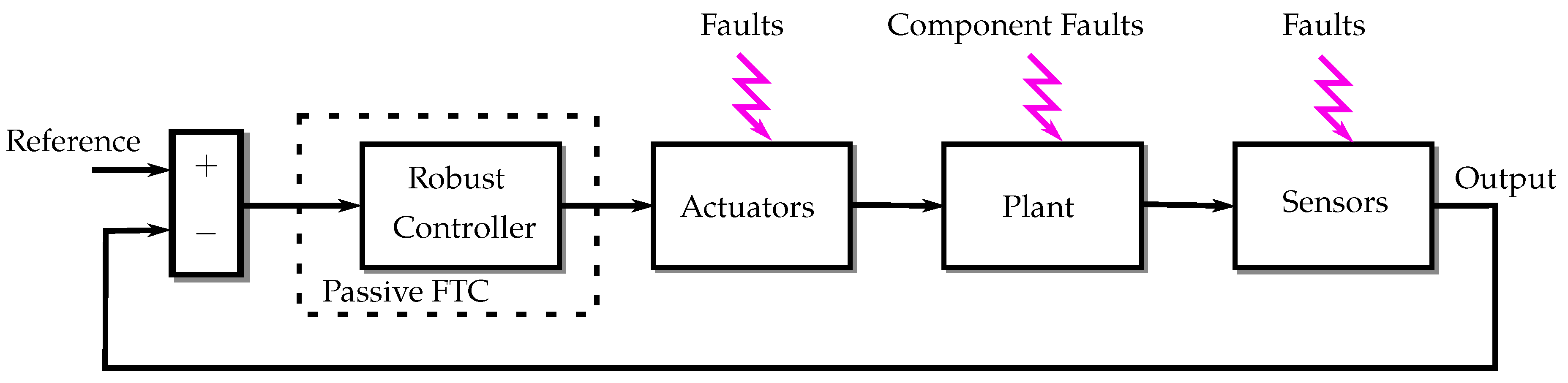
• Passive techniques consider that possible system failures are known. The controller is thus developed to cover the a priori known characteristics of a set of pre-specified faults. Given that the controller stays fixed during the systems operation, this makes passive approaches less complex, considering that the robustness properties of the so-designed controller are exploited (see Figure 4). As a consequence, the type of faults that the robust controller can compensate is limited. However, their lack of complexity is an advantage during implementation, given that they have fewer software/hardware requirements.
• Active techniques reconfigure the control parameters in the presence of a fault. They rely on a Fault Detection and Isolation (FDI) unit (see Figure 5). FDI is in charge of the constant monitoring of the status of the system and its components. In this way, when the FDI unit identifies a fault, a reconfiguration is carried out in the controller. As a result, a wider range of faults can be compensated and many control techniques have the potential to be used for fault tolerant control, e.g., $H_{\infty }$ both within the LTI and linear parameter varying setting, control allocation, dynamic inversion, adaptive methods, neural networks, and model predictive control, to mention a few. One limitation of this scheme is that it has limited time to perform FDI followed by control reconfiguration. In addition, the accuracy of FDI affects the reconfiguration process. In other words, despite the existence of some stability and performance proofs for active FTC techniques, the main problem lies in guaranteeing stability and performances of the overall fault-tolerant scheme taking into account FDI performances (detection delay, possible false alarms, etc.), control specifications, and reconfiguration mechanism. Solutions to this problem are considered in [56,57]. The authors proposed to use the theory of switched systems based on the dwell-time concept to guarantee stability and fault accommodation, even in the case of false fault identification.

In the following, we restrict our discussion to the application of SMC techniques to the FTC problem. The interested reader can refer to the works in [51,52,53,54,55] (and references therein) for good surveys.

5.1. Modeling the Faults

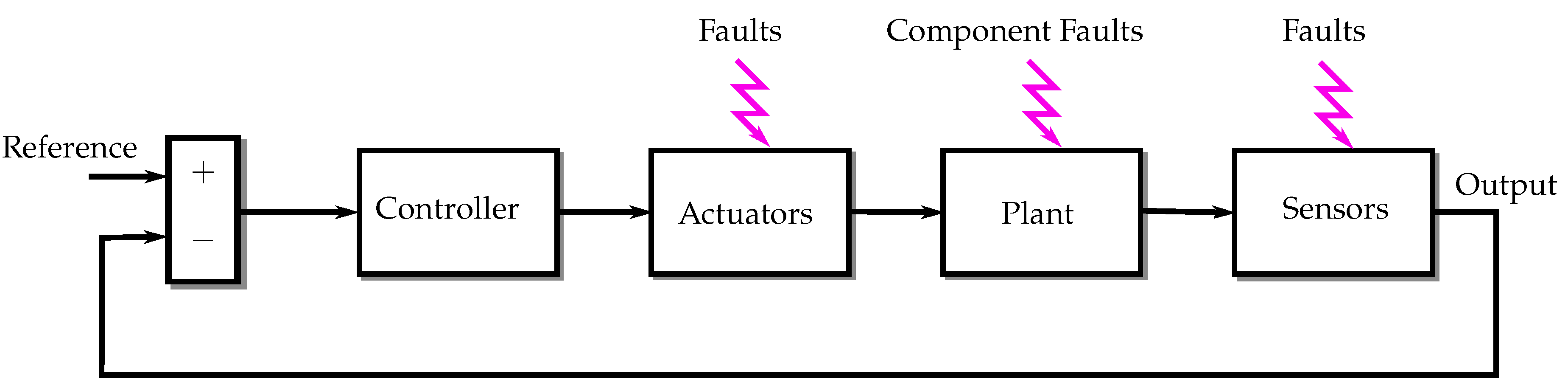
According to their location, faults can be classified as sensor, actuator, or component faults, as shown in Figure 6. Sensor and actuator faults can present total or partial loss. A total loss on an actuator represents a stuck actuator that does not generate the expected actuation, despite the applied input. For the case of a sensor, it means that the received measurements are incorrect. Furthermore, an actuator with partial loss produces a percentage of the expected actuation. In the sensor case, the measurements may be noisier, scaled, or have an offset. Component faults represent changes in physical parameters which affect the dynamical behavior of the system. Component faults are hard to classify and enumerate, since they can cover a wide variety of situations.

Faults can be modeled according to additive or multiplicative representations. The description of a component fault is translated to a modification on the system’s matrix. For the Linear Time-Invariant (LTI) case, it is modeled as:

$$\dot{x}\left(t\right)=A_{f}x\left(t\right)+Bu\left(t\right)=(A+\Delta A)x\left(t\right)+Bu\left(t\right)$$

(74)

where $A\in {\mathbb{R}}^{n\times n},B\in {\mathbb{R}}^{n\times m}$. $\Delta A\in {\mathbb{R}}^{n\times n}$ represents a change in the system matrix A, leading the model (74) to be a multiplicative fault model.

An offset or drift in the control signal can be described as an additive signal according to

$$u_f\left(t\right)=u\left(t\right)+f\left(t\right)$$

(75)

where $f\left(t\right)\in {\mathbb{R}}^m$ represents the fault profile and $u_f\left(t\right)\in {\mathbb{R}}^m$ is the faulty control input. Since $f\left(t\right)$ acts directly on the state equation, this actuator fault model results in an additive fault representation. On the other hand, multiplicative actuator faults can be described as [58,59,60,61]

$$u_f\left(t\right)=(\mathbb{I}-\Psi \left(t\right))u\left(t\right)$$

(76)

where $\Psi \left(t\right)=\mathrm{diag}[{\psi }_1\left(t\right),\dots ,{\psi }_n\left(t\right)]$ is a (time-dependent) unknown matrix that has values that range between $[0,1]$, so that ${\psi }_i\left(t\right)=0\forall t$ represents normal actuation. This formalism covers a large variety of fault profiles. When ${\psi }_i\left(t\right)=1fort\ge t_f$, the ith actuator becomes out of order for $t\ge t_f$. ${\psi }_i\left(t\right)=\%x$ for $t\ge t_f$ means a loss of efficiency for time $t\ge t_f$. ${\psi }_i\left(t\right)=1-{\varphi }_i\left(t\right)/u_i\left(t\right)$ for $t\ge t_f$ indicates that the behavior of the ith actuator is imposed by the time-dependent function ${\varphi }_i\left(t\right)$ for $t\ge t_f$, and thus its motion becomes equal to $\varphi \left(t\right)$ for time $t\ge t_f$, leading the actuator uncontrollable. As an example, the polynomial ${\varphi }_i\left(t\right)={\sum }_{k=1}^m{a}_k{t}^k$ for $t\ge t_f$ can be used to model stuck open/closed faults occurring in the ith actuator at time $t_f$.

It is worth noting that, using an additive approximation of the fault multiplicative fault models (74) and (76), the dynamics of the faulty system can be written according to [55,58,62]

$$\dot{x}\left(t\right)=Ax\left(t\right)+Bu\left(t\right)+\sum _i{H}_{a,i}{f}_i\left(t\right)$$

(77)

where the ith column of the matrix $H_a$ is the ith fault signature associated to the ith fault mode $f_i\left(t\right)$. Note that, depending on the nature of the faults, $f_i\left(t\right)$ may depend on the states $x\left(t\right)$, i.e., $f_i(x\left(t\right),t)$, and thus stability of the FTC solution must be carefully addressed in this case.

Similar expressions are obtained for describing faulty measurements $y_f\left(t\right)$ caused by faulty sensors. The difference relies on changing $u\left(t\right)$ and $u_f\left(t\right)$ for $y\left(t\right)$ and $y_f\left(t\right)$ in (75) for additive fault type models and (76) for multiplicative fault type models, respectively. Another possibility which is often used in sliding mode fault tolerant control community is to consider sensor fault as a virtual actuator additive fault [21,63]. To proceed, consider a linear system affected by sensor faults

$$\begin{array}{cc}\hfill & \dot{x}\left(t\right)=Ax\left(t\right)+Bu\left(t\right)\hfill \end{array}$$

(78)

$$\begin{array}{cc}\hfill & y_f\left(t\right)=Cx\left(t\right)+H_{s}f\left(t\right)\hfill \end{array}$$

(79)

where $A\in {\mathbb{R}}^{n\times n},B\in {\mathbb{R}}^{n\times m}$ and $H_s\in {\mathbb{R}}^{p\times q}$ with $q<p\le n$. Here, $H_s$ represents the sensor fault distribution matrix and it is assumed to be of rank q. The signal $f\left(t\right)$ is assumed to be continuously differentiable and unknown, but subject to $\left|\right|f\left(t\right)\left|\right|\le \beta$. Let us split $y_f\left(t\right)$ according to

$$\left[\begin{array}{c}{y}_1\left(t\right)\\ y_{f,2}\left(t\right)\end{array}\right]=\left[\begin{array}{c}{C}_1\\ C_2\end{array}\right]x\left(t\right)+\left[\begin{array}{c}0\\ {\mathbb{I}}_q\end{array}\right]f\left(t\right)$$

(80)

where $C_1$ has full row rank. In this equation, $y_{f,2}\left(t\right)$ denotes the outputs which are potentially corrupted by sensor faults whereas the subset, whereas $y_1\left(t\right)$ are fault free. Define a (stable) fault model in the form

$${\dot{z}}_f\left(t\right)=-A_f{z}_f\left(t\right)+A_f{y}_{f,2}\left(t\right)$$

(81)

where $z_f\left(t\right)\in {\mathbb{R}}^q$ and the matrix $A_f\in {\mathbb{R}}^{q\times q}$ is positive definite. From (78), (79), and (81), the following augmented system with state ${\left[x^T{z}_f^T\right]}^T$, can be defined

$$\left[\begin{array}{c}\dot{x}\left(t\right)\hfill \\ {\dot{z}}_f\left(t\right)\end{array}\right]=\left[\begin{array}{cc}A& 0\\ A_f{C}_2& -A_f\end{array}\right]\left[\begin{array}{c}x\left(t\right)\\ z_f\left(t\right)\end{array}\right]+\left[\begin{array}{c}B\\ 0\end{array}\right]u\left(t\right)+\left[\begin{array}{c}0\\ A_f\end{array}\right]f\left(t\right)$$

(82)

$$\left[\begin{array}{c}{y}_1\left(t\right)\hfill \\ z_f\end{array}\right]u\left(t\right)=\left[\begin{array}{cc}{C}_1& 0\\ 0& {\mathbb{I}}_q\end{array}\right]\left[\begin{array}{c}x\left(t\right)\\ z_f\left(t\right)\end{array}\right]$$

(83)

Exploiting the fact that the rows of $C_1$ are rows from ${\mathbb{I}}_n$, there exists a coordinate transformation matrix

$$T_e=diag\left(T,{\mathbb{I}}_q\right),T\in {\mathbb{R}}^{n\times n},C_1{T}^{-1}=\left[\begin{array}{cc}0& {\mathbb{I}}_{p-q}\end{array}\right]$$

(84)

such that, in the new coordinate system, the augmented plant (82) and (83) has the form

$$\begin{array}{cc}\hfill & {\dot{x}}_e\left(t\right)=A_e{x}_e\left(t\right)+B_{e}u\left(t\right)+D_{e}f\left(t\right)\hfill \end{array}$$

(85)

$$\begin{array}{cc}\hfill & y_e\left(t\right)=C_e{x}_e\left(t\right)\hfill \end{array}$$

(86)

where $x_e\in {\mathbb{R}}^{n+q},y_e={\left[y_1^T{z}_f^T\right]}^T$, $D_e={\left[0A_f^T\right]}^T$ and $C_e=\left[0{\mathbb{I}}_p\right]$. This model finally results in a virtual additive actuator fault model where the fault $f\left(t\right)$ is distributed through $D_e$.

In a very similar fashion, it is proposed in [64,65] to use a different formulation for the fault model (81), i.e.,

$$\begin{array}{cc}\hfill & {\dot{z}}_f\left(t\right)=A_f{z}_f\left(t\right)+w\left(t\right)\hfill \end{array}$$

(87)

$$\begin{array}{cc}\hfill & f\left(t\right)=z_f\left(t\right)\hfill \end{array}$$

(88)

where $w\left(t\right)\in {\mathbb{R}}^q$ is an unknown signal so that $\left|\right|w\left(t\right)\left|\right|\le \beta$. Then, the technique consist in considering the fault dynamics as a part of an extended vector $x_e={\left[x^T{z}_f^T\right]}^T$ with the following associated state space model

$${\dot{x}}_e\left(t\right)=\left[\begin{array}{cc}A& 0\\ 0& A_f\end{array}\right]x_e\left(t\right)+\left[\begin{array}{c}B\\ 0\end{array}\right]u\left(t\right)+\left[\begin{array}{c}0\\ {\mathbb{I}}_q\end{array}\right]w\left(t\right)$$

(89)

$$y_f\left(t\right)=\left[\begin{array}{cc}C\hfill & H_s\end{array}\right]x_e\left(t\right)$$

(90)

which is equivalent to considering the sensor faults as virtual actuator additive faults through the distribution matrix $\left[\begin{array}{c}0\\ {\mathbb{I}}_q\end{array}\right]$.

5.2. SMC Techniques as a Potential Solution for FTC

Coming back to the models (77), (85), (86), (89), and (90), it seems obvious that a unified representation can be established for any kind of faults, according to

$$\begin{array}{cc}\hfill & \dot{x}\left(t\right)=Ax\left(t\right)+Bu\left(t\right)+Kf(x\left(t\right),t)\hfill \end{array}$$

(91)

$$\begin{array}{cc}\hfill & y\left(t\right)=Cx\left(t\right)\hfill \end{array}$$

(92)

where matrices $A,B,K,C$ take the adequate definition, given the considered faults. It is now apparent that the SMC techniques described in Section 4.1, Section 4.2 and Section 4.3 may be suitable, when applied to (91) and (92), de facto solving the FTC problem. The key ingredient is the definition of the matrix K and the signal $f\left(x\right(t),t)$. Typically,

• If $K=B$, then $Bu\left(t\right)+Kf\left(x\right(t),t)=B\left(u\right(t)+f(x\left(t\right),t\left)\right)$; thus, it is immediate to see that from the FTC point of view that we are facing a large class of actuator faults since the fault profile f may be state-dependent. A particular case often encountered in the literature consists of faults being exogenous signals, i.e., $f=f\left(t\right)$. From the SMC point of view, f can be treated as (state-dependent) matched perturbations.
• If $Kf(x\left(t\right),t)={\sum }_i{H}_{a,i}{f}_i\left(t\right)=H_{a}f\left(t\right)$ as in (77), then $K=H_a,f=f\left(t\right)$; thus, we are faced with actuator faults where the ith column of K represents the fault mode of the ith actuator. From the SMC point of view, f is seen as unmatched perturbations.
• If $Kf\left(x\right(t),t)=\Delta Ax\left(t\right)$, then the problem is concerned by component faults (see (74)). From a SMC point of view, we are facing unmatched perturbations.
• If $K={\left[0A_f^T\right]}^T$ or $K={\left[0{\mathbb{I}}_q\right]}^T$, then it is immediate to see from (85), (86), (89), and (90) that, from the FTC point of view, we are faced with sensor faults that have been reformulated as virtual actuator faults. From the SMC point of view, we are faced with unmatched perturbations.

In this sense, (91) and (92) represent a unified model to tackle the FTC problem in a unified manner using SMC approaches. Thus, depending on the definition of $Kf\left(x\right(t),t)$:

• If f plays the role of matched perturbations, the control theories presented in Section 4.1, Section 4.2 and Section 4.3 can be applied with a few changes. That is why active and passive SMC-based FTC schemes have be proposed in the literature (see, e.g., [66,67,68,69,70,71] for passive and [72,73,74,75,76] for active FTC solutions). However, tuning the gains of the tSMC control law to ensure fault tolerance may lead to a high gain controller. This is in fact related to the outcomes discussed below about the assumption on $f\left(t\right)$ and its successive time derivatives, and the problem of control saturation.
• If f plays the role of unmatched perturbations, it is required to use a fault reconstruction unit. This can be done by using either a (high-order sliding mode) observer or a differentiator on an adequate formulated problem (see Section 4.2.6 and Section 4.3.1). The models (77), (85), (86), (89), and (90) are generally used for that purpose (for studies that use this principle, see [18,48,64,65,77,78,79,80,81,82,83,84,85,86,87]).

Nevertheless, and for evident stability issues, particular care must be taken when f depends on the state x. For such cases, VGSTA or GSTA must be used.

Although there exist fundamental properties that lead the application of SMC techniques to the FTC problem. In the authors’ opinion, based on the discussion above, the following open problems still exist:

• First, the following assumptions must be satisfied: $\left(i\right)$ the system (91)–(92) must be strongly observable, or, equivalently, the triplet $(A,C,K)$ has no invariant zeros; and $\left(ii\right)$ depending on the SMC technique used for FTC and fault reconstruction, f and its derivatives up to a certain order (say r) may be bounded, i.e., $∥f^{\left(i\right)}∥\le {\beta }_i$, $i=0,...,r$, or $f\left(t\right)$ must be smooth at least.
• Second, because many SMC techniques are state-feedback control solutions, the state $x\left(t\right)$ must be available. However, controllers such as the nested algorithm and quasi-continuous sliding-mode controller only require the relative degree and the measurement of one of the state variables.
• Third, fault accommodation is done at the expense of increasing the control actions, which may lead the control signal to go into saturation.

The first problem is not solved. The reason sliding modes are usually restricted to smooth fault profiles comes from the necessity of providing smooth estimates of the fault. The sliding mode is extended considering the first derivative of the fault and a continuous injection term of the observer can be used for exact fault reconstruction in finite-time. It is also possible to consider a discontinuous fault profile. However, in this case, if it is desired to use the equivalent output injection to reconstruct the fault, this reconstruction will require the application of a filter, providing only an asymptotic estimation of the fault. That is why almost all papers that deal with FTC with SMC techniques restrict the time profile of f to a smooth profile, such as loss of effectiveness fault type or sinusoidal behavior (see the following section that reviews the most common applications of SMC for FTC in real-world systems). The problem becomes challenging when considering abrupt and/or discontinuous faults. Lan and Patton [87] presented some interesting results in this sense. In this paper, f is considered nowhere differentiable, but it is worth noting that f is still assumed to be smooth.

If the fault (and its successive time derivatives) is assumed to be bounded, most of the current SMC theories for FTC assume that these bounds are not known, which is a reasonable assumption from a practical point of view since fault characteristics cannot be known a priori. Thus, following the discussion presented in Section 4.4, the ASMC principle is the most studied technique in the literature. We recall that this approach consist of the use of a SMC unit, which is scheduled by a fault estimator in charge of estimating the required characteristics (such as the bound value) of the faults. Different ASMC strategies have been proposed (see Section 5.3 that presents an overview of current applications). However, it is worth noting that the strong assumption about the continuity of the fault profile is not yet relaxed.

If the second problem admits solutions by using, e.g., observers or differentiators (see Section 4.2.6 and Section 4.3.1), there does not really exist a proof of a kind of separation principle. That is why the solution consists in waiting for the convergence of the observer or differentiator, and then turning on the control. A solution to this problem is studied in [87] by using adaptive gain for the observer and the adaptive back-stepping control technique.

The third problem can be approached by using an anti-windup scheme. Instability of a SMC-based FTC law occurs due to control saturation, especially for the SMC techniques that use an integral term, e.g., ISMC, STA, or GSTA [88,89,90].

For instance, if (48) is directly used as the control law, saturation caused by the integral term ${\int }_0^t{k}_2\mathrm{sign}\left(x\right)d\tau$ may lead to instability of the closed-loop. The simplest anti-windup solution thus consists in introducing an anti-windup coefficient $e^{-\Lambda (u_{sat}-u)}$ so that (48) is rewritten according to

$$u\left(t\right)=-{\left(SB\right)}^{-1}\left[SAx\left(t\right)+k_1{\left|x\right|}^{\frac{1}{2}}\mathrm{sign}\left(x\right)+e^{-\Lambda (u_{sat}\left(t\right)-u\left(t\right))}{\int }_0^t{k}_2\mathrm{sign}\left(x\right)d\tau \right]$$

(93)

where $\Lambda$ is a diagonal matrix with strict positive terms ${\lambda }_i$ and where $u_{sat}\left(t\right)=sat\left(u\left(t\right)\right)$. When no saturation occurs, $u_{sat}\left(t\right)=u\left(t\right)$ and the anti-windup coefficient $e^{-\Lambda (u_{sat}\left(t\right)-u\left(t\right)}$ equals the identity, vanishing its effect in (93), and thus (93) equals (48). When the difference between $u\left(t\right)$ and $u_{sat}\left(t\right)$ is large enough, since $\Lambda >0$, $e^{-\Lambda (u_{sat}\left(t\right)-u\left(t\right))}$ is near zero according to the property of the exponential function, and the integral term, which is responsible of the instability, vanishes from the control signal. In addition, the overshoot of the closed-loop due to saturation can be reduced to different degrees through changing the values of $\Lambda$. The same technique is also valid for VGSTA and GSTA, which results in introducing the anti-windup coefficient $e^{-\Lambda (u_{sat}\left(t\right)-u\left(t\right)}$ in (54) and (56), respectively.

However, if such an anti-windup strategy has been observed useful in practice, there does not exist a formal proof of stability, when the anti-windup coefficient operates, i.e., when the time-varying weighting term $e^{-\Lambda (u_{sat}\left(t\right)-u\left(t\right)}$ takes (continuously) its values between $[0,1]$. This is still an open problem.

A solution may consist of the anti-windup strategy proposed in [90], but it is limited to STA. Furthermore, it is restricted to the particular class of faults (75), for f being bounded and composed of two components $f_1$ and $f_2$ that are Hölder continuous in the state and Lipschitz continuous in time, respectively, i.e., $f=f_1+f_2$ with $\left|f\right|\le W,|f_1|\le K\sqrt{\left|x\right|},\left|{\dot{f}}_2\right|\le L$. $W,K$, and L are non-negative constants. The solution, called saturated STA, consists of the following control for the discontinuous part of STA

$$\begin{array}{cc}\hfill & u_n=sat\left(-k_1{\left|x\right|}^{\frac{1}{2}}sign\left(x\right)+v\right)\hfill \end{array}$$

(94)

$$\dot{v}=\left\{\begin{array}{cc}0\hfill & |u_n|=u^{+}\hfill \\ -k_{2}sign\left(x\right)\hfill & |u_n|<u^{+}\hfill \end{array}\right.$$

(95)

with $K<k_1-\sqrt{2L+2k_2}$ and $W<u^{+}\frac{k_1^2-K{k}_1-2k_2}{k_1^2-K{k}_1+2k_2}$, where $u^{+}$ is the control saturation level. Then, when saturation occurs, $\dot{v}=0$, vanishing the integral term in (94). This principle relies on the same principle than the one used in (93) through the anti-windup coefficient, but, as opposed to (93), the anti-windup solution (94) and (95) has the disadvantage of requiring some assumptions about the fault $f\left(t\right)$ but the advantage of being formally proved stable.

5.3. Applications of SMC for FTC in Real-World Systems

Looking at the current literature, one can identify four main application domains of SMC for FTC: $\left(i\right)$ robot manipulators; $\left(ii\right)$ marine vehicles (including ships, surface and underwater vehicles); $\left(iii\right)$ aeronautics (this includes unmanned aerial vehicles); and $\left(iv\right)$ satellites/spacecraft. The following subsections discuss the recent results in these application domains. Note that, besides the studies discussed in the following subsections, there are other applications reported in the literature. The focuses of these applications are out of or far away from the scope of this section. However, it is interesting to note the work reported in [91] where a higher-order sliding mode based control scheme is proposed for the air path of a diesel engine, and that in [92] for air-to-fuel ratio fault tolerance based on a smooth STA for a gasoline engine.

5.3.1. Robot Manipulators

In [93], tracking SMC algorithm is investigated for robot manipulators with emphasis on unsurity, faults compromising tendency and fluctuations rejection. The work reported in [94,95] presents two FTC solutions for robot manipulators, based on synchronous TSM controller and an extended state observer. The finite-time synchronization technique makes both the joint position error and the synchronization error converge to zero, in finite time, while considering the robot singularity avoidance problem. Fault tolerance against robot manipulator faults with singularity avoidance is considered in [96] using a combination of STA, disturbance estimation, and non-singular fast TSM controller. According to the authors, the proposed solution has the advantages of reducing the transient performance, convergence in short time, and rejection of the chattering phenomenon. Furthermore, since it uses a disturbance estimator, which provides de facto fault estimation (see our discussion in Section 5.2), prior information about upper bound values of faults is not required. Based on the nonsingular fast TSM control technique reported in [97] and starting from the selection of an integral nonsingular fast terminal sliding surface, the work presented in [93] proposes an integral nonsingular fast terminal sliding mode controller, used in a back-stepping configuration. Again, the FTC principle lies on the use of a fault estimator which is performed by means of time delay estimation. The convergence speed of the conventional TSM depends on the initial state values, which provides a longer convergence time when the initial state values are big. The fixed-time SMC technique provides a solution to this problem (see [98,99]). This motivated the work presented in [100]. The method again shares the same principle as the previous FTC solutions: use a disturbance/fault estimator to provide disturbance/fault bounds that are further injected as parameters in a SMC law. In this paper, the estimates are provided by means of a fixed-time super-twisting sliding mode observer and the SMC law results in a fixed-time sliding mode controller.

5.3.2. Marine Vehicles

In the field of marine vehicles/marine surface vessels, most recent SMC-FTC papers focus on actuator faults. Two kinds of solutions have been proposed: $\left(i\right)$ control allocation coupled with a SMC law to ensure tracking performance and disturbance/uncertainties rejection; and $\left(ii\right)$ ASMC schemes.

The FTC solution proposed in [101] obeys to the first category of solutions. Based on the precursor study proposed in [102], an actuator weight matrix is introduced in the allocation unit and the corresponding element is adjusted in accordance with the thruster fault information provided by a fault diagnosis unit to reduce the priority of the faulty thruster. At the same time, the fault information is used to schedule the gains of the SMC unit. One of the major advantage, is that actuators saturation can be considered, thanks to the control allocation unit.

In contrast to the control-allocation FTC principle, the following solutions are based on ASMC schemes. We recall that for such FTC solutions, the main concept is based on a fault estimator. The FTC scheme presented in [103] relies an a ASMC approach under some $H_{\infty }$ performance and has the advantage to cover state time-delay, as opposed to [104], as well as a large class of actuator fault types. The FTC principle relies on an adaptive mechanism of the sliding-mode controller. The FTC solution proposed in [105] employs a finite-time fault tolerant estimator to identify actuator faults online that is incorporated in an integral sliding-mode controller. However, faults are assumed to be twice differentiable. In a very similar fashion, the solution presented in [106] is based on an adaptive TSM solution. An adaptive adjustment technique is proposed to estimate online the bound of the change of thrust distribution gain resulted from thruster fault. In [107], an adaptive sliding mode observer is constructed by combining a linear function, signature function, integral function, and a fractional-order function of the position estimation error. The integral SMC technique is then used for control. Motivated by faster convergence capacities in reaching and sliding phase and the convergence of the steady-state error to a small region, a fixed-time velocity-free sliding mode tracking control scheme is used for FTC against actuator faults in [108]. However, the control parameters are numerous and not easy to adjust. The concept of fixed-time SMC is also used in [109] in a feedback sliding mode tracking control scheme to tackle the problem of time-varying disturbances, unmeasurable velocities, unmodeled dynamics, and actuator faults. The fault tolerance principle relies on the use of a singularity-free fixed-time sliding mode control law. Finally, Yao [110] proposed an adaptive finite-time SMC scheme that consists in combining the homogeneous integral sliding mode manifold, fast TSM control, and an adaptation technique. One of the major advantages is that control input saturation is considered.

5.3.3. Aeronautical Applications

The problem of designing FTC schemes for quadrotor Unmanned Aerial Vehicle (UAV)s has been widely studied during this last decade, with a particular focus on motor/propeller faults. Many solutions consider only partial loss, simply because a complete loss of a motor/propeller of the quadrotor leads to the inability to fully control the UAV’s attitude [111]. Due to this difficulty, there are only a few works considering the case of complete rotor loss using SMC approaches (see, e.g., [112]). All existing solutions sacrifice the controllability of the yaw angle to still be able to command the UAV’s position and altitude by making it continuously rotate around its “z-axis”. The alternative consists of the use of more actuated UAVs, e.g., octorotor UAVs. For instance, two SMC-FTC solutions are investigated in [113]. The first solution relies on a robust adaptive sliding mode Control Allocation (CA) where the control gains of the controller are adjusted online in order to redistribute the control signals among the healthy motors. The second solution is based on a self-tuning SMC, where the control gains are readjusted depending on the detected error to maintain the stability of the system. The solutions proposed in [114,115] consist of the combination of ISMC and CA techniques, to redistribute control signals on fault-free motors.

Partial loss of motor/propeller is thus the most encountered studied faulty situation. The solutions reported in [70,116,117,118,119] propose passive SMC-based FTC solutions. However, in such schemes, the magnitude of faults is designed in a given boundary. To overcome this limitation, active FTC solutions have been proposed. In [120,121], an observer for sate and/or fault estimation is proposed that is injected into the sliding mode controller for reconfiguration. The solution discussed in [122] shares the same strategy. Based on the initial work reported in [119], a $H_{\infty }$ observer is used to estimate (time-varying) faults, which are then injected into an adaptive sliding mode back-stepping control scheme. One of the great advantage of the proposed approach is that it can handle control saturations. In [123], an ASMC scheme is presented, where a fixed-time extended state observer is utilized to estimate states, lumped disturbances, and actuator fault information. Nevertheless, the disadvantage is that the parameter called the switching time cannot be adjusted. In [124,125], the FTC solutions rely on robust and adaptive control laws based on sliding mode and back-stepping theories to compensate the effectiveness loss in actuators. The solution proposed in [126] is based on a continuous fast nonsingular TSM controller, augmented with an adaptive finite-time extended state observer. As opposed to the authors of [127,128,129] who developed finite-time extended state observers, where large gains are employed because of the lumped disturbances unknown bounds, an adaptive procedure is developed with less conservativeness. The fault control principle consists of a continuous fast nonsingular TSM controller, retained due to its fast response and robustness to uncertainties, and it accommodates actuator faults in a finite time as well. The continuous TA is used in [130] for fault tolerance of motor faults of a 3-DoF helicopter prototype. A FDI unit is proposed based on the dynamic model of the helicopter, the inputs, the outputs, and some of its derivatives, provided in finite time by third-order sliding mode differentiators, which schedules the continuous twisting controller, ensuring de facto, fault tolerance.

Notable contributors who develop FTC strategies for aircraft actuator and sensor faults using SMC schemes, are Edwards, Alwi and co-workers. These authors also proposed solutions with validation on industrial integration benches, iron-bird platforms, and real flight tests, mostly with the support of the AIRBUS aircraft manufacturer and the Japan Aerospace Exploration Agency’s (JAXA’s) Multipurpose Aviation Laboratory. For instance, it is demonstrated in [63,131] that the combination of ISMC and the ability of CA to redistribute control signals leads to a single controller that handles both nominal fault-free and fault conditions, without changing the structure of the already in-place controller. This is useful since flight envelop protection (e.g., load factor protection, angle-of-attack protection. etc.) can be guaranteed by the operation of the already in-place controller. The method presented in [132,133] also shares the same philosophy. The ISMC law is retrofitted to the already in-place controller, and, at the same time, a CA unit redistributes the control signal to fault free control surfaces, when faults have been identified by a FDI unit. The proposed solutions are however based on a LTI model of the (faulty) aircraft. This motivated the authors to extend their approach to the Linear Parameter Varying (LPV) setting [134,135,136,137,138], with flight tests presented in [76]. It is interesting to note that, in [135], a LPV sliding-mode observer is used for both actuator and sensor faults in a unified fashion, through the concept of output injection, as explained in Section 5.2. The work reported in [139] differs a little bit from the aforementioned solutions, in the sense that a LPV-based model reference FTC scheme is proposed to recover faults in aircraft control surfaces. However, the proposed solution still uses jointly SMC and CA techniques.

5.3.4. Space Applications

The last domain of application of SMC for FTC concerns space missions, due to the evident need of high autonomy, especially for deep space missions. For such missions, the delay of telemetry communications with Earth stations could lead the mission in danger, on-board FTC solutions are required. The problem of spacecraft attitude tracking subject to actuator faults is, for instance, addressed in [140,141]. Fault tolerance against actuator faults is ensured using adaptive nonsingular TSM control technique. In [129], a FTC solution is addressed by integrating a finite-time extended state observer into a fast nonsingular TSM controller, to estimate and compensate for the specified synthetic uncertainties derived from actuator failures and/or model deviations. In [142], a fixed-time sliding mode manifold is proposed for the attitude’s control of spacecraft subject to actuator saturation and faults. The solution proposed in [143] uses a fuzzy logic system to estimate (approximate to be more precise) the external disturbances and faults. The estimates are re-injected into a fractional order SMC law that uses a double power exponential reaching law and the back-stepping control approach. A similar approach based on neural network and an adaptive first-order SMC approach is used in [144]. The proposed solution also protects the control law from actuator position saturation with globally asymptotically attitude tracking. The work reported in [145] investigates the FTC problem of spacecraft rendezvous and docking with a freely tumbling target in the presence of thruster loss-of-efficiency fault types. The proposed solution uses a passive FTC-SMC solution that guarantees fixed-time reachability of the system states into the small neighborhood of the designed fixed-time sliding mode in the presence of actuator faults and external disturbances. In [146], an active fault tolerant controller is designed by using both the classical back-stepping control scheme and ISMC technique. An adaptive non-linear fault estimation observer is designed in order to obtain the estimated value of unknown time-varying faults. The work reported in [71] is also based on a ISMC technique. By means of one-parameter dependent adaptive mechanism, it is shown that the closed-loop system is capable of tolerating potential actuator faults without requiring any information on the boundaries of disturbances and faults, except for their existence. A passive FTC approach is presented in [147] based on the fast TSM control approach. The proposed solution not only has the ability to protect the actuator from saturation but also guarantees that attitude and angular velocity converge to a neighborhood of the origin in finite time. In [148], a passive FTC approach is proposed using a nonsingular fixed-time TSM control scheme, formulated as a prescribed performance control problem. It is proved that the attitude of the spacecraft is kept within the predefined constraint boundaries, even when the actuator saturation is taken into account. An anti-unwinding finite time fault tolerant sliding mode control solution is also considered in [149]. The solution reported in [150] considers the attitude’s FTC problem under uncertainties and control saturation, by means of a fast nonsingular TSM technique and fuzzy logic rules. Differently from the work in [151,152], the proposed solution can handle actuator failures and saturations in a less conservative manner, according to the authors. The work reported in [153] ensures fault tolerance by means of a nonlinear ISMC technique. The proposed approach uses an adaptive fault observer and a control gain adaption method, based on dual-layer gain adaptation scheme [154]. Finally, in [155], the authors proposed an integral terminal sliding-mode controller such that the sliding motion realizes the action of a quaternion-based nonlinear proportional-derivative controller. Adaptive techniques are used to tackle uncertainties, and the resultant adaptive SMC law stabilizes the system states to a small neighborhood around the sliding surface, in finite time.

Another space application that has recently received attention considers re-entry vehicles. The work reported in [156] is based on sliding mode observer technique and fuzzy control to tackle the problem of actuator faults. The solution proposed in [157] is based on a decentralized asymptotic FTC system to ensure attitude fault performance, by means of SMC, command filter and back-stepping techniques. In [158,159], the proposed solution relies on a ASMC law, structured into inner and outer loops. A nonlinear fault detection observer is used to detect a fault, which enables to engage the FTC law. The work reported in [160] considers an adaptive-gain multivariable observer to estimate partial loss of actuator effectiveness. The estimates are then combined with a second-order sliding mode controller based on the TSM technique and STA. Finally, Chang et al. [50] proposed a super-twisting sliding mode observer to estimate actuator faults, that is combined with a model-reference ISMC law. A interesting property of the proposed method is that it manages control signal saturation as well as undesirable transient behavior by means of a bumpless strategy.

5.3.5. Notable Facts

From the above review of current applications of SMC for FTC to real-world system, it is worth noting that:

• Almost all current SMC-based FTC solutions are based on the ASMC principle, as described in Section 5.2, i.e., a fault estimator is used to schedule a SMC law. It is interesting to note that the most popular control scheme is the TSM control solution and its variants, i.e., the fast and nonsingular fast versions.
• Many papers do not consider the problem of control signal saturation. The majority of contributions in this field are developed for space applications.
• No papers (or almost none) have proposed a solution to relax the assumption about the discontinuity of the fault profile. The considered faults are manly concerned by loss-of-efficiency or smooth fault profiles.
• Finally, no papers have established a formal proof of the existence of a separation principle when using a fault estimator, even if it is mainly used as the fault tolerance principle. This means that the coupling between the dynamics of the fault estimator and the SMC law is not sufficiently studied, in our opinion.

6. Conclusions

This paper reviews the five generations of Sliding Mode Control (SMC) techniques, with the underlying goal to identify the techniques that can be used for Fault-Tolerant Control (FTC). Operating principles and concepts of SMC solutions are presented, and details are given when the technique is judged applicable to the FTC problem. Fault models are established and discussed with the objective to obtain models suitable for SMC techniques. It is shown that the major future challenges in this field are concerning:

(i)

the case of discontinuous faults, since, by definition, such faults do not respect the assumption about the bound required by the sliding-mode controller to maintain the sliding-motion, and to not test again a transient process of finite-duration;

(ii)

the proof of stability when an anti-windup strategy is joint to the SMC architecture (when such a unit is considered, which is rarely the case); and

(iii)

the non-existence of a separation principle when using a fault estimator.

References

- Yu, X.; Jiang, J. A survey of fault-tolerant controllers based on safety-related issues. Annu. Rev. Control 2015, 39, 46–57. [Google Scholar] [CrossRef]
- Sato, M.; Hardier, G.; Ferreres, G.; Edwards, C.; Alwi, H.; Chen, L.; Marcos, A. Fault Tolerance - Background and Recent Trends. J. Soc. Instrum. Control. Eng. 2018, 57, 279–286. [Google Scholar] [CrossRef]
- Amin, A.A.; Hasan, K.M. A review of Fault Tolerant Control Systems: Advancements and applications. Measurement 2019, 143, 58–68. [Google Scholar] [CrossRef]
- Abbaspour, A.; Mokhtari, S.; Sargolzaei, A.; Yen, K.K. A Survey on Active Fault-Tolerant Control Systems. Electronics 2020, 9, 1513. [Google Scholar] [CrossRef]
- Riaz, U.; Tayyeb, M.; Amin, A.A. A Review of Sliding Mode Control with the Perspective of Utilization in Fault Tolerant Control. Recent Adv. Electr. Electron. Eng. 2020, 13, 1–13. [Google Scholar] [CrossRef]
- Levant, A. Universal single-input-single-output (SISO) sliding-mode controllers with finite-time convergence. IEEE Trans. Autom. Control 2001, 46, 1447–1451. [Google Scholar] [CrossRef] [Green Version]
- Shtessel, Y.; Edwards, C.; Fridman, L.; Levant, A. Sliding Mode Control and Observation; Springer: Berlin/Heidelberg, Germany, 2014; Volume 10. [Google Scholar]
- Fridman, L.; Moreno, J.A.; Bandyopadhyay, B.; Kamal, S.; Chalanga, A. Continuous nested algorithms: The fifth generation of sliding mode controllers. In Recent Advances in Sliding Modes: From Control to Intelligent Mechatronics; Springer: Berlin/Heidelberg, Germany, 2015; pp. 5–35. [Google Scholar]
- Emel’yanov, S. On Pecularities of Variables Structure Control Systems with Discontinuous Switching Functions; Doklady ANSSR: Moscow, Russia, 1963; Volume 153, pp. 776–778. [Google Scholar]
- Emelyanov, S. Variable Structure Control Systems; Nauka: Moscow, Russia, 1967. (In Russian) [Google Scholar]
- Utkin, V. Variable structure systems with sliding modes. IEEE Trans. Autom. Control 1977, 22, 212–222. [Google Scholar] [CrossRef]
- Utkin, V.I. Sliding Modes and Their Applications in Variable Structure Systems; Mir Publishers: Moscow, Russia, 1978; p. 257. [Google Scholar]
- Feng, Y.; Yu, X.; Han, F. On nonsingular terminal sliding-mode control of nonlinear systems. Automatica 2013, 49, 1715–1722. [Google Scholar] [CrossRef]
- Davila, J. Exact tracking using backstepping control design and high-order sliding modes. IEEE Trans. Autom. Control 2013, 58, 2077–2081. [Google Scholar] [CrossRef]
- Davila, J.; Fridman, L.; Pisano, A.; Usai, E. Finite-time state observation for non-linear uncertain systems via higher-order sliding modes. Int. J. Control 2009, 82, 1564–1574. [Google Scholar] [CrossRef]
- Yan, X.G.; Edwards, C. Nonlinear robust fault reconstruction and estimation using a sliding mode observer. Automatica 2007, 43, 1605–1614. [Google Scholar] [CrossRef]
- Utkin, V.I. Sliding Modes in Control and Optimization; Springer Science & Business Media: Berlin/Heidelberg, Germany, 2013. [Google Scholar]
- Edwards, C.; Spurgeon, S. Sliding Mode Control: Theory and Applications; CRC Press: Boca Raton, FL, USA, 1998. [Google Scholar]
- Matthews, G.; DeCarlo, R. Decentralized tracking for a class of interconnected nonlinear systems using variable structure control. Automatica 1988, 24, 187–193. [Google Scholar] [CrossRef]
- Utkin, V.; Shi, J. Integral sliding mode in systems operating under uncertainty conditions. In Proceedings of the Conference on Decision and Control, Kobe, Japan, 13 December 1996; pp. 4591–4596. [Google Scholar]
- Hamayun, M.T.; Edwards, C.; Alwi, H. Fault Tolerant Control Schemes Using Integral Sliding Modes; Springer: Berlin/Heidelberg, Germany, 2016. [Google Scholar]
- Castanos, F.; Fridman, L. Analysis and Design of Integral Sliding Manifolds for Systems With Unmatched Perturbations. IEEE Trans. Autom. Control. 2006, 51, 853–858. [Google Scholar] [CrossRef] [Green Version]
- Bezzaoucha, S.; Henry, D. An LMI approach for the Integral Sliding Mode and H∞ State Feedback Control Problem. J. Phys. Conf. Ser. 2015, 659, 012052. [Google Scholar] [CrossRef]
- Chalanga, A.; Kamal, S.; Bandyopadhyay, B. Continuous integral sliding mode control: A chattering free approach. In Proceedings of the 2013 IEEE International Symposium on Industrial Electronics, Taipei, Taiwan, 28–31 May 2013; pp. 1–6. [Google Scholar]
- Kamal, S.; Chalanga, A.; Bandyopadhyay, B.; Kumar P, R. Multivariable continuous integral sliding mode control. In Proceedings of the 2015 International Workshop on Recent Advances in Sliding Modes (RASM), Istanbul, Turkey, 9–11 April 2015; pp. 1–5. [Google Scholar]
- Levant, A. Higher Order Sliding Modes and Their Application for Controlling Uncertain Processes; Institute for System Studiesof the USSR Acadamy of Science: Moscow, Russia, 1987. [Google Scholar]
- Emel’yanov, S.V.; Korovin, S.; Levantovskii, L.V. Higher-order sliding modes in binary control systems. Sov. Phys. Dokl. 1986, 31, 291. [Google Scholar]
- Venkataraman, S.; Gulati, S. Control of nonlinear systems using terminal sliding modes. J. Dyn. Sys. Meas. Control 1993, 115, 554–560. [Google Scholar] [CrossRef]
- Levant, A. Sliding order and sliding accuracy in sliding mode control. Int. J. Control. 1993, 58, 1247–1263. [Google Scholar] [CrossRef]
- Moreno, J.A.; Osorio, M. Strict Lyapunov functions for the super-twisting algorithm. IEEE Trans. Autom. Control 2012, 57, 1035–1040. [Google Scholar] [CrossRef]
- Levant, A. Robust exact differentiation via sliding mode technique. Automatica 1998, 34, 379–384. [Google Scholar] [CrossRef]
- Gonzalez, T.; Moreno, J.A.; Fridman, L. Variable gain super-twisting sliding mode control. IEEE Trans. Autom. Control 2011, 57, 2100–2105. [Google Scholar] [CrossRef]
- Moreno, J.A. A linear framework for the robust stability analysis of a Generalized Super-Twisting Algorithm. In Proceedings of the 2009 6th International Conference on Electrical Engineering, Computing Science and Automatic Control (CCE), Toluca, Mexico, 10–13 January 2009; pp. 1–6. [Google Scholar]
- Castillo, I.; Fridman, L.; Moreno, J.A. Super-Twisting Algorithm in presence of time and state dependent perturbations. Int. J. Control 2018, 91, 2535–2548. [Google Scholar] [CrossRef]
- Levant, A. Introduction to high-order sliding modes. Sch. Math. Sci. Isr. 2003, 58, 1. [Google Scholar]
- Emelyanov, S. Higher order sliding modes in the binary control systems. Sov. Phys. Dokl. 1986, 4, 291–293. [Google Scholar]
- Feng, Y.; Yu, X.; Man, Z. Non-singular terminal sliding mode control of rigid manipulators. Automatica 2002, 38, 2159–2167. [Google Scholar] [CrossRef]
- Yu, X.; Zhihong, M. Fast terminal sliding-mode control design for nonlinear dynamical systems. IEEE Trans. Circuits Syst. I Fundam. Theory Appl. 2002, 49, 261–264. [Google Scholar]
- Seeber, R.; Horn, M. Stability proof for a well-established super-twisting parameter setting. Automatica 2017, 84, 241–243. [Google Scholar] [CrossRef]
- Seeber, R.; Horn, M. Necessary and sufficient stability criterion for the super-twisting algorithm. In Proceedings of the 2018 15th International Workshop on Variable Structure Systems (VSS), Graz, Austria, 9–11 July 2018; pp. 120–125. [Google Scholar] [CrossRef]
- Levant, A. Higher-order sliding modes, differentiation and output-feedback control. Int. J. Control 2003, 76, 924–941. [Google Scholar] [CrossRef]
- Huang, Y.J.; Kuo, T.C.; Chang, S.H. Adaptive sliding-mode control for nonlinearsystems with uncertain parameters. IEEE Trans. Syst. Man Cybern. Part B Cybern. 2008, 38, 534–539. [Google Scholar] [CrossRef] [PubMed]
- Emelyanov, S.; Utkin, V.; Taran, V. Theory of systems with variable structure. Science 1970. [Google Scholar]
- Shtessel, Y.B.; Moreno, J.A.; Plestan, F.; Fridman, L.M.; Poznyak, A.S. Super-twisting adaptive sliding mode control: A Lyapunov design. In Proceedings of the 49th IEEE Conference on Decision and Control (CDC), Atlanta, GA, USA, 15–17 December 2010; pp. 5109–5113. [Google Scholar]
- Harmouche, M.; Laghrouche, S.; Chitour, Y. Robust and adaptive higher order sliding mode controllers. In Proceedings of the 2012 IEEE 51st IEEE Conference on Decision and Control (CDC), Maui, HI, USA, 10–13 December 2012; pp. 6436–6441. [Google Scholar]
- Taleb, M.; Levant, A.; Plestan, F. Pneumatic actuator control: Solution based on adaptive twisting and experimentation. Control Eng. Pract. 2013, 21, 727–736. [Google Scholar] [CrossRef]
- González, J.A.; Barreiro, A.; Dormido, S.; Banos, A. Nonlinear adaptive sliding mode control with fast non-overshooting responses and chattering avoidance. J. Frankl. Inst. 2017, 354, 2788–2815. [Google Scholar] [CrossRef]
- Hmidi, R.; Brahim, A.B.; Hmida, F.B.; Sellami, A. Robust Fault Tolerant Control Design for Nonlinear Systems not Satisfying Matching and Minimum Phase Conditions. Int. J. Control Autom. Syst. 2020, 18, 2206–2219. [Google Scholar] [CrossRef]
- Efimov, D.; Edwards, C.; Zolghadri, A. Enhancement of adaptive observer robustness applying sliding mode techniques. Automatica 2016, 72, 53–56. [Google Scholar] [CrossRef] [Green Version]
- Chang, J.; Cieslak, J.; Guo, Z.; Henry, D. On the synthesis of a sliding-mode-observer-based adaptive fault-tolerant flight control scheme. ISA Trans. 2020. [Google Scholar] [CrossRef]
- Blanke, M.; Staroswiecki, M.; Wu, N. Concepts and methods in fault-tolerant control. In Proceedings of the 2001 American Control Conference, Arlington, VA, USA, 25–27 June 2001. [Google Scholar]
- Lunze, J.; Richter, J. Control Reconfiguration: Survey of Methods and Open Problems; Technical Report; Ruhr-Universität Bochum, Lehrstuhl für Automatisierungstechnik und Prozessinformatik: Bochum, Germany, 2006. [Google Scholar]
- Zhang, Y.; Jiang, J. Bibliographical review on reconfigurable fault-tolerant control systems. Ann. Rev. Control 2008, 32, 229–252. [Google Scholar] [CrossRef]
- Blanke, M.; Kinnaert, M.; Lunze, M.; Staroswiecki, M. Diagnosis and Fault Tolerant Control; Springer: Berlin/Heidelberg, Germany, 2006. [Google Scholar]
- Zolghadri, A.; Henry, D.; Cieslak, J.; Efimov, D.; Goupil, P. Fault Diagnosis and Fault-Tolerant Control and Guidance for Aerospace Vehicles: From Theory to Application; Advances in Industrial Control; Springer: Berlin/Heidelberg, Germany, 2014; ISBN 978-1-4471-5312-2. [Google Scholar]
- Efimov, D.; Cieslak, J.; Henry, D. Supervisory fault-tolerant control with mutual performance optimization. Int. J. Adapt. Control. Signal Process. 2013, 27, 251–279. [Google Scholar] [CrossRef]
- Cieslak, J.; Efimov, D.; Henry, D. Transient management of a supervisory fault-tolerant control scheme based on dwell-time conditions. Int. J. Adapt. Control. Signal Process. 2015, 29, 123–142. [Google Scholar] [CrossRef]
- Henry, D. Fault Diagnosis of the Microscope Satellite Actuators using H∞/H_ Filters. AIAA J. Guid. Control. Dyn. 2008, 31, 699–711. [Google Scholar] [CrossRef]
- Henry, D. From fault diagnosis to recovery actions for aeronautic and aerospace missions: A model-based point of view. In Proceedings of the 23rd IAR Workshop on Advanced Control and Diagnosis, Coventry, UK, 27–28 November 2008. [Google Scholar]
- Henry, D. A norm-based point of view for fault diagnosis. Application to aerospace missions. In Proceedings of the 8th European Workshop on Advanced Control and Diagnosis, Ferrara, Italy, 18–19 November 2010; pp. 4–16. [Google Scholar]
- Fonod, R.; Henry, D.; Charbonnel, C.; Bornschlegl, E.; Losa, D.; Bennani, S. Robust FDI for fault-tolerant thrust allocation with application to spacecraft rendezvous. Control. Eng. Pract. 2015, 42, 12–27. [Google Scholar] [CrossRef]
- Frank, P.; Alcorta-Garcia, E.; Köppen-Seliger, B. Modelling for fault detection and Isolation versus Modelling for Control. Math. Comput. Model. Dyn. Syst. 2001, 7, 1–46. [Google Scholar] [CrossRef]
- Edwards, C.; Lombaerts, T.; Smaili, H. Fault Tolerant Flight Control: A Benchmark Challenge; Springer: Berlin/Heidelberg, Germany, 2010. [Google Scholar]
- Ferreira De Loza, A.; Cieslak, J.; Henry, D.; Dávila, J.; Zolghadri, A. Sensor fault diagnosis using a non-homogeneous high-order sliding mode observer with application to a transport aircraft. IET Control Theory Appl. 2015, 598–607. [Google Scholar] [CrossRef]
- Ferreira, A.; Cieslak, J.; Henry, D.; Zolghadri, A.; Fridman, L. Output tracking of systems subjected to perturbations and a class of actuator faults based on HOSM observation and identification. Automatica 2014, 59, 200–205. [Google Scholar] [CrossRef]
- Liu, C.; Jiang, B.; Patton, R.J.; Zhang, K. Decentralized Output Sliding-Mode Fault-Tolerant Control for Heterogeneous Multiagent Systems. IEEE Trans. Cybern. 2019, 50, 4934–4945. [Google Scholar] [CrossRef]
- Lan, J.; Patton, R.J. Integrated fault estimation and fault-tolerant control for uncertain Lipschitz nonlinear systems. Int. J. Robust Nonlinear Control 2017, 27, 761–780. [Google Scholar] [CrossRef]
- Lan, J.; Patton, R.J. A new strategy for integration of fault estimation within fault-tolerant control. Automatica 2016, 69, 48–59. [Google Scholar] [CrossRef]
- Davila, J.; Cieslak, J.; Henry, D.; Zolghadri, A.; Bejarano, F.J. A fault tolerant controller based on quasi-continuous high-order sliding mode technique. In Proceedings of the 2016 American Control Conference (ACC), Boston, MA, USA, 6–8 July 2016; pp. 7529–7534. [Google Scholar]
- Merheb, A.R.; Noura, H.; Bateman, F. Design of passive fault-tolerant controllers of a quadrotor based on sliding mode theory. Int. J. Appl. Math. Comput. Sci. 2015, 25, 561–576. [Google Scholar] [CrossRef] [Green Version]
- Shen, Q.; Wang, D.; Zhu, S.; Poh, E.K. Integral-Type Sliding Mode Fault-Tolerant Control for Attitude Stabilization of Spacecraft. IEEE Trans. Control. Syst. Technol. 2015, 23, 1131–1138. [Google Scholar] [CrossRef]
- Hamayun, M.T.; Edwards, C.; Alwi, H. Design and analysis of an integral sliding mode fault-tolerant control scheme. IEEE Trans. Autom. Control 2011, 57, 1783–1789. [Google Scholar] [CrossRef] [Green Version]
- Xu, S.S.D.; Chen, C.C.; Wu, Z.L. Study of nonsingular fast terminal sliding-mode fault-tolerant control. IEEE Trans. Ind. Electron. 2015, 62, 3906–3913. [Google Scholar] [CrossRef]
- Chen, L.; Alwi, H.; Edwards, C. Development and evaluation of an integral sliding mode fault-tolerant control scheme on the RECONFIGURE benchmark. Int. J. Robust Nonlinear Control 2019, 29, 5314–5340. [Google Scholar] [CrossRef]
- Chen, L.; Edwards, C.; Alwi, H. Integral sliding mode fault-tolerant control allocation for a class of affine nonlinear system. Int. J. Robust Nonlinear Control 2019, 29, 565–582. [Google Scholar] [CrossRef]
- Chen, L.; Edwards, C.; Alwi, H.; Sato, M. Flight evaluation of a sliding mode online control allocation scheme for fault tolerant control. Automatica 2020, 114, 108829. [Google Scholar] [CrossRef]
- Edwards, C.; Spurgeon, S.K.; Patton, R.J. Sliding mode observers for fault detection and isolation. Automatica 2000, 36, 541–553. [Google Scholar] [CrossRef]
- Chen, L.; Alwi, H.; Edwards, C. On the synthesis of an integrated active LPV FTC scheme using sliding modes. Automatica 2019, 110, 108536. [Google Scholar] [CrossRef]
- Yin, S.; Yang, H.; Kaynak, O. Sliding mode observer-based FTC for Markovian jump systems with actuator and sensor faults. IEEE Trans. Autom. Control 2017, 62, 3551–3558. [Google Scholar] [CrossRef]
- Chu, Z.; Meng, F.; Zhu, D.; Luo, C. Fault reconstruction using a terminal sliding mode observer for a class of second-order MIMO uncertain nonlinear systems. ISA Trans. 2020, 97, 67–75. [Google Scholar] [CrossRef] [PubMed]
- Xiao, B.; Yin, S.; Gao, H. Reconfigurable tolerant control of uncertain mechanical systems with actuator faults: A sliding mode observer-based approach. IEEE Trans. Control. Syst. Technol. 2017, 26, 1249–1258. [Google Scholar] [CrossRef]
- Ferrara, A.; Incremona, G.P.; Sangiovanni, B. Sliding Mode Fault Diagnosis with Vision in the Loop for Robot Manipulators. In New Trends in Robot Control; Springer: Berlin/Heidelberg, Germany, 2020; pp. 81–105. [Google Scholar]
- Ríos, H.; Kamal, S.; Fridman, L.M.; Zolghadri, A. Fault tolerant control allocation via continuous integral sliding-modes: A HOSM-observer approach. Automatica 2015, 51, 318–325. [Google Scholar] [CrossRef]
- Dávila, J.; Cieslak, J.; Henry, D. Disturbance Observer-Based Fault-Tolerant Control for a Class of Additive Faults. In New Trends in Observer-Based Control; Elsevier: Amsterdam, The Netherlands, 2019; pp. 337–355. [Google Scholar]
- Chang, J.; Cieslak, J.; Davila, J.; Zolghadri, A.; Zhou, J. Analysis and design of second-order sliding-mode algorithms for quadrotor roll and pitch estimation. ISA Trans. 2017, 71, 495–512. [Google Scholar] [CrossRef]
- Chang, J.; Cieslak, J.; Dávila, J.; Zhou, J.; Zolghadri, A.; Guo, Z. A two-step approach for an enhanced quadrotor attitude estimation via IMU data. IEEE Trans. Control. Syst. Technol. 2017, 26, 1140–1148. [Google Scholar] [CrossRef]
- Lan, J.; Patton, R.J. A decoupling approach to integrated fault-tolerant control for linear systems with unmatched non-differentiable faults. Automatica 2018, 89, 290–299. [Google Scholar] [CrossRef]
- Castillo, I.; Steinberger, M.; Fridman, L.; Moreno, J.; Horn, M. Saturated Super-Twisting Algorithm based on Perturbation Estimator. In Proceedings of the 2016 IEEE 55th Conference on Decision and Control (CDC), Las Vegas, NV, USA, 12–14 December 2016; pp. 7325–7328. [Google Scholar] [CrossRef]
- Golkani, M.A.; Koch, S.; Reichhartinger, M.; Horn, M. A novel saturated super-twisting algorithm. Syst. Control. Lett. 2018, 119, 52–56. [Google Scholar] [CrossRef]
- Seeber, R.; Horn, M. Guaranteeing Disturbance Rejection and Control Signal Continuity for the Saturated Super-Twisting Algorithm. IEEE Control Syst. Lett. 2019, 3, 715–720. [Google Scholar] [CrossRef] [Green Version]
- Murtaza, G.; Butt, Y.A.; Bhatti, A.I. Higher order sliding mode based control scheme for air path of diesel engine. In Proceedings of the 2016 International Conference on Emerging Technologies (ICET), Balaclava, Mauritius, 3–6 August 2016; pp. 1–6. [Google Scholar] [CrossRef]
- Anjum, R.; Khan, I.; Yar, A.; Bhatti, A.I. Air-to-fuel ratio control of gasoline engines using smooth sliding mode algorithm. In Proceedings of the 2017 13th International Conference on Emerging Technologies (ICET), Islamabad, Pakistan, 27–28 December 2017; pp. 1–6. [Google Scholar] [CrossRef]
- Van, M.; Mavrovouniotis, M.; Ge, S.S. An Adaptive Backstepping Nonsingular Fast Terminal Sliding Mode Control for Robust Fault Tolerant Control of Robot Manipulators. IEEE Trans. Syst. Man Cybern. Syst. 2019, 49, 1448–1458. [Google Scholar] [CrossRef] [Green Version]
- Lee, Q.; Kang, H. Finite-Time Fault-Tolerant Control for a Robot Manipulator Based on Synchronous Terminal Sliding Mode Control. Appl. Sci. 2020, 10, 2998. [Google Scholar] [CrossRef]
- Lee, Q.; Kang, H. Implementation of Fault-Tolerant Control for a Robot Manipulator Based on Synchronous Sliding Mode Control. Appl. Sci. 2020, 10, 2534. [Google Scholar] [CrossRef] [Green Version]
- Vo, A.T.; Kang, H. A Novel Fault-Tolerant Control Method for Robot Manipulators Based on Non-Singular Fast Terminal Sliding Mode Control and Disturbance Observer. IEEE Access 2020, 8, 109388–109400. [Google Scholar] [CrossRef]
- Van, M.; Ge, S.S.; Ren, H. Finite Time Fault Tolerant Control for Robot Manipulators Using Time Delay Estimation and Continuous Nonsingular Fast Terminal Sliding Mode Control. IEEE Trans. Cybern. 2017, 47, 1681–1693. [Google Scholar] [CrossRef]
- Li, H.; Cai, Y. On SFTSM control with fixed-time convergence. IET Control. Theory Appl. 2017, 11, 766–773. [Google Scholar] [CrossRef]
- Basin, M.; Panathula, C.B.; Shtessel, Y. Multivariable continuous fixed-time second-order sliding mode control: Design and convergence time estimation. IET Control. Theory Appl. 2017, 11, 1104–1111. [Google Scholar] [CrossRef]
- Van, M.; Ceglarek, D. Robust fault tolerant control of robot manipulators with global fixed-time convergence. J. Frankl. Inst. 2021, 358, 699–722. [Google Scholar] [CrossRef]
- Lv, T.; Zhou, J.; Wang, Y.; Gong, W.; Zhang, M. Sliding mode based fault tolerant control for autonomous underwater vehicle. Ocean Eng. 2020, 216, 107855. [Google Scholar] [CrossRef]
- Lakhekar, G.; Waghmare, L. Robust maneuvering of autonomous underwater vehicle: An adaptive fuzzy PI sliding mode control. Intell. Serv. Robot. 2017, 10, 195–212. [Google Scholar] [CrossRef]
- Hao, L.Y.; Zhang, H.; Li, H.; Li, T.S. Sliding mode fault-tolerant control for unmanned marine vehicles with signal quantization and time-delay. Ocean Eng. 2020, 215, 107882. [Google Scholar] [CrossRef]
- Hao, L.; Zhang, H.; Guo, G.; Li, H. Quantized Sliding Mode Control of Unmanned Marine Vehicles: Various Thruster Faults Tolerated With a Unified Model. IEEE Trans. Syst. Man, Cybern. Syst. 2019, 1–15. [Google Scholar] [CrossRef]
- Wang, N.; Pan, X.; Su, S.F. Finite-time fault-tolerant trajectory tracking control of an autonomous surface vehicle. J. Frankl. Inst. 2020, 357, 11114–11135. [Google Scholar] [CrossRef]
- Zhang, M.; Liu, X.; Yin, B.; Liu, W. Adaptive terminal sliding mode based thruster fault tolerant control for underwater vehicle in time-varying ocean currents. J. Frankl. Inst. 2015, 352, 4935–4961. [Google Scholar] [CrossRef]
- Liu, X.; Zhang, M.; Wang, Y.; Rogers, E. Design and Experimental Validation of an Adaptive Sliding Mode Observer-Based Fault-Tolerant Control for Underwater Vehicles. IEEE Trans. Control. Syst. Technol. 2019, 27, 2655–2662. [Google Scholar] [CrossRef]
- Zhang, J.; Yu, S.; Yan, Y. Fixed-time velocity-free sliding mode tracking control for marine surface vessels with uncertainties and unknown actuator faults. Ocean Eng. 2020, 201, 107107. [Google Scholar] [CrossRef]
- Zhang, J.; Yu, S.; Yan, Y.; Wu, D. Fixed-time output feedback sliding mode tracking control of marine surface vessels under actuator faults with disturbance cancellation. Appl. Ocean Res. 2020, 104, 102378. [Google Scholar] [CrossRef]
- Yao, Q. Adaptive finite-time sliding mode control design for finite-time fault-tolerant trajectory tracking of marine vehicles with input saturation. J. Frankl. Inst. 2020, 357, 13593–13619. [Google Scholar] [CrossRef]
- Lanzon, A.; Freddi, A.; Longhi, S. Flight Control of a Quadrotor Vehicle Subsequent to a Rotor Failure. J. Guid. Control. Dyn. 2014, 37, 580–591. [Google Scholar] [CrossRef]
- Khattab, A.; Alwi, H.; Edwards, C. Mitigating total rotor failure in quadrotor using LPV based sliding mode control scheme. In Proceedings of the 2019 4th Conference on Control and Fault Tolerant Systems (SysTol), Casablanca, Morocco, 18–20 September 2019; pp. 98–103. [Google Scholar] [CrossRef]
- Hamadi, H.; Lussier, B.; Fantoni, I.; Francis, C.; Shraim, H. Comparative study of self tuning, adaptive and multiplexing FTC strategies for successive failures in an Octorotor UAV. Robot. Auton. Syst. 2020, 133, 103602. [Google Scholar] [CrossRef]
- Alwi, H.; Hamayun, M.T.; Edwards, C. An integral sliding mode fault tolerant control scheme for an octorotor using fixed control allocation. In Proceedings of the 2014 13th International Workshop on Variable Structure Systems (VSS), Nantes, France, 29 June–2 July 2014; pp. 1–6. [Google Scholar] [CrossRef]
- Alwi, H.; Edwards, C. Fault tolerant control of an octorotor using LPV based sliding mode control allocation. In Proceedings of the 2013 American Control Conference, Washington, DC, USA, 17–19 June 2013; pp. 6505–6510. [Google Scholar] [CrossRef]
- Wang, B.; Zhang, Y. Adaptive Sliding Mode Fault-Tolerant Control for an Unmanned Aerial Vehicle. Unmanned Syst. 2017, 5, 209–221. [Google Scholar] [CrossRef]
- Merheb, A.; Noura, H.; Bateman, F. Passive fault tolerant control of quadrotor UAV using regular and cascaded Sliding Mode Control. In Proceedings of the 2013 Conference on Control and Fault-Tolerant Systems (SysTol), Nice, France, 9–11 October 2013; pp. 330–335. [Google Scholar] [CrossRef]
- Li, T.; Zhang, Y.; Gordon, B.W. Passive and active nonlinear fault-tolerant control of a quadrotor unmanned aerial vehicle based on the sliding mode control technique. Proc. Inst. Mech. Eng. Part I J. Syst. Control. Eng. 2013, 227, 12–23. [Google Scholar] [CrossRef]
- Nguyen, N.P.; Hong, S.K. Fault-tolerant Control of Quadcopter UAVs Using Robust Adaptive Sliding Mode Approach. Energies 2018, 12, 95. [Google Scholar] [CrossRef] [Green Version]
- Sharifi, F.; Mirzaei, M.; Gordon, B.W.; Zhang, Y. Fault tolerant control of a quadrotor UAV using sliding mode control. In Proceedings of the 2010 Conference on Control and Fault-Tolerant Systems (SysTol), Nice, France, 6–8 October 2010; pp. 239–244. [Google Scholar] [CrossRef]
- Merheb, A.; Noura, H.; Bateman, F. Active fault tolerant control of quadrotor UAV using Sliding Mode Control. In Proceedings of the 2014 International Conference on Unmanned Aircraft Systems (ICUAS), Orlando, FL, USA, 27–30 May 2014; pp. 156–166. [Google Scholar] [CrossRef]
- Nguyen, N.P.; Hong, S.K. Active Fault-Tolerant Control of a Quadcopter against Time-Varying Actuator Faults and Saturations Using Sliding Mode Backstepping Approach. Appl. Sci. 2019, 9, 4010. [Google Scholar] [CrossRef] [Green Version]
- Zhang, L.; Wei, C.; Wu, R.; Cui, N. Adaptive fault-tolerant control for a VTVL reusable launch vehicle. Acta Astronaut. 2019, 159, 362–370. [Google Scholar] [CrossRef]
- Avram, R.C.; Zhang, X.; Muse, J. Nonlinear Adaptive Fault-Tolerant Quadrotor Altitude and Attitude Tracking With Multiple Actuator Faults. IEEE Trans. Control. Syst. Technol. 2018, 26, 701–707. [Google Scholar] [CrossRef]
- Song, Z.; Sun, K. Attitude Tracking Control of A Quad-Rotor with Partial Loss of Rotation Effectiveness. Asian J. Control 2017, 19, 1812–1821. [Google Scholar] [CrossRef]
- Tang, P.; Lin, D.; Zheng, D.; Fan, S.; Ye, J. Observer based finite-time fault tolerant quadrotor attitude control with actuator faults. Aerosp. Sci. Technol. 2020, 104, 105968. [Google Scholar] [CrossRef]
- Shi, D.; Wu, Z.; Chou, W. Super-Twisting Extended State Observer and Sliding Mode Controller for Quadrotor UAV Attitude System in Presence of Wind Gust and Actuator Faults. Electronics 2018, 7, 128. [Google Scholar] [CrossRef] [Green Version]
- Li, B.; Hu, Q.; Yang, Y. Continuous finite-time extended state observer based fault tolerant control for attitude stabilization. Aerosp. Sci. Technol. 2019, 84, 204–213. [Google Scholar] [CrossRef]
- Li, B.; Hu, Q.; Yu, Y.; Ma, G. Observer-Based Fault-Tolerant Attitude Control for Rigid Spacecraft. IEEE Trans. Aerosp. Electron. Syst. 2017, 53, 2572–2582. [Google Scholar] [CrossRef]
- Pérez-Ventura, U.; Fridman, L.; Capello, E.; Punta, E. Fault tolerant control based on continuous twisting algorithms of a 3-DoF helicopter prototype. Control Eng. Pract. 2020, 101, 104486. [Google Scholar] [CrossRef]
- Alwi, H.; Edwards, C. Fault tolerant control using sliding modes with on-line control allocation. Automatica 2008, 44, 1859–1866. [Google Scholar] [CrossRef] [Green Version]
- Alwi, H.; Edwards, C. A fault tolerant integral sliding mode control allocation scheme for the RECONFIGURE benchmark problem. In Proceedings of the 2014 American Control Conference, Portland, OR, USA, 4–6 June 2014; pp. 660–665. [Google Scholar] [CrossRef]
- Chandra, K.P.B.; Chen, L.; Alwi, H.; Edwards, C. Actuator faults and blow-down limit detection, and fault tolerant control for the RECONFIGURE benchmark problem. In Proceedings of the 2016 IEEE Conference on Control Applications (CCA), Buenos Aires, Argentina, 19–22 September 2016; pp. 1544–1549. [Google Scholar] [CrossRef]
- Chen, L.; Alwi, H.; Edwards, C. Application and evaluation of an LPV integral sliding mode fault tolerant control scheme on the RECONFIGURE benchmark. In Proceedings of the 2016 American Control Conference (ACC), Boston, MA, USA, 6–8 July 2016; pp. 3692–3697. [Google Scholar] [CrossRef]
- Chandra, K.P.B.; Chen, L.; Alwi, H.; Edwards, C. Development and evaluation of sliding mode schemes for the RECONFIGURE benchmark problem. In Proceedings of the 2016 3rd Conference on Control and Fault-Tolerant Systems (SysTol), Barcelona, Spain, 7–9 September 2016; pp. 805–810. [Google Scholar] [CrossRef]
- Chen, L.; Alwi, H.; Edwards, C.; Sato, M. Evaluation of a Sliding Mode Fault Tolerant Controller on the MuPAL-α Research Aircraft. In Proceedings of the 2018 IEEE Conference on Control Technology and Applications (CCTA), Copenhagen, Denmark, 21–24 August 2018; pp. 760–765. [Google Scholar] [CrossRef] [Green Version]
- Chen, L.; Alwi, H.; Edwards, C.; Sato, M. Active Fault Tolerant Control of MuPAL-a Using Sliding Modes. In Proceedings of the 2018 Annual American Control Conference (ACC), Milwaukee, WI, USA, 27–29 June 2018; pp. 6120–6125. [Google Scholar] [CrossRef] [Green Version]
- Vile, L.; Alwi, H.; Edwards, C. Scheduled Fault Tolerant Integral Sliding Mode Control for BWB Aircraft. In Proceedings of the 2020 European Control Conference (ECC), Saint Petersburg, Russia, 12–15 May 2020; pp. 1903–1908. [Google Scholar] [CrossRef]
- Alwi, H.; Chen, L.; Edwards, C. Application of an LPV based Model Reference FTC Scheme on the RECONFIGURE benchmark model. In Proceedings of the 2018 Annual American Control Conference (ACC), Milwaukee, WI, USA, 27–29 June 2018; pp. 5332–5337. [Google Scholar] [CrossRef]
- Han, Z.; Zhang, K.; Yang, T. Spacecraft attitude control using nonsingular finite-time convergence Terminal Sliding Mode. In Proceedings of the 2016 IEEE Chinese Guidance, Navigation and Control Conference (CGNCC), Nanjing, China, 12–14 August 2016; pp. 618–623. [Google Scholar] [CrossRef]
- Jing, C.; Xu, H.; Niu, X.; Song, X. Adaptive Nonsingular Terminal Sliding Mode Control for Attitude Tracking of Spacecraft With Actuator Faults. IEEE Access 2019, 7, 31485–31493. [Google Scholar] [CrossRef]
- Jiang, B.; Hu, Q.; Friswell, M.I. Fixed-Time Attitude Control for Rigid Spacecraft With Actuator Saturation and Faults. IEEE Trans. Control. Syst. Technol. 2016, 24, 1892–1898. [Google Scholar] [CrossRef]
- Qian, M.; Shi, Y.; Gao, Z.; Zhang, X. Integrated fault tolerant tracking control for rigid spacecraft using fractional order sliding mode technique. J. Frankl. Inst. 2020, 357, 10557–10583. [Google Scholar] [CrossRef]
- Xiao, B.; Hu, Q.; Zhang, Y. Adaptive Sliding Mode Fault Tolerant Attitude Tracking Control for Flexible Spacecraft Under Actuator Saturation. IEEE Trans. Control. Syst. Technol. 2012, 20, 1605–1612. [Google Scholar] [CrossRef]
- Jiang, B.; Hu, Q.; Friswell, M.I. Fixed-time rendezvous control of spacecraft with a tumbling target under loss of actuator effectiveness. IEEE Trans. Aerosp. Electron. Syst. 2016, 52, 1576–1586. [Google Scholar] [CrossRef] [Green Version]
- Gao, Z.; Zhou, Z.; Qian, M.; Lin, J. Active fault tolerant control scheme for satellite attitude system subject to actuator time-varying faults. IET Control Apilication 2018, 12, 405–412. [Google Scholar] [CrossRef]
- Shen, Q.; Wang, D.; Zhu, S.; Poh, K. Finite-time fault-tolerant attitude stabilization for spacecraft with actuator saturation. IEEE Trans. Aerosp. Electron. Syst. 2015, 51, 2390–2405. [Google Scholar] [CrossRef]
- Golestani, M.; Esmaeilzadeh, S.M.; Xiao, B. Fault-tolerant attitude control for flexible spacecraft subject to input and state constraint. Trans. Inst. Meas. Control 2020, 42, 2660–2674. [Google Scholar] [CrossRef]
- Shahna, M.H.; Abedi, M. An anti-unwinding finite time fault tolerant sliding mode control of a satellite based on accurate estimation of inertia moments. ISA Trans. 2020, 101, 23–41. [Google Scholar] [CrossRef] [PubMed]
- Gao, S.; Jing, Y.; Liu, X.; Zhang, S. Finite-time attitude-tracking control for rigid spacecraft with actuator failures and saturation constraints. Int. J. Robust Nonlinear Control 2020, 30, 1903–1937. [Google Scholar] [CrossRef]
- Lu, K.; Xia, Y. Finite-time fault-tolerant control for rigid spacecraft with actuator saturations. IET Control Theo. Appl. 2013, 11, 1529–1539. [Google Scholar] [CrossRef]
- Lu, K.; Xia, Y.; Fu, M.; Yu, C. Adaptive finite-time attitude stabilization for rigid spacecraft with actuator faults and saturation constraints. Int. J. Robust Nonlinear Control 2016, 26, 28–46. [Google Scholar] [CrossRef]
- Hu, H.; Liu, L.; Wang, Y.; Cheng, Z.; Luo, Q. Active fault-tolerant attitude tracking control with adaptive gain for spacecrafts. Aerosp. Sci. Technol. 2020, 98, 105706. [Google Scholar] [CrossRef]
- Edwards, C.; Shtessel, Y. Adaptive dual-layer super-twisting control and observation. Int. J. Control 2016, 89, 1759–1766. [Google Scholar] [CrossRef] [Green Version]
- Gui, H.; Vukovich, G. Adaptive fault-tolerant spacecraft attitude control using a novel integral terminal sliding mode. Int. J. Robust Nonlinear Control 2017, 27, 3174–3196. [Google Scholar] [CrossRef]
- Xu, Y.; Jiang, B.; Tao, G.; Gao, Z. Fault Accommodation For Near Space Hypersonic Vehicle With Actuator Fault. Int. J. Innov. Comput. Inf. Control. 2011, 7, 2187–2200. [Google Scholar]
- Xu, D.; Jiang, B.; Liu, H.; Shi, P. Decentralized asymptotic fault tolerant control of near space vehicle with high order actuator dynamics. J. Frankl. Inst. 2013, 350, 2519–2534. [Google Scholar] [CrossRef]
- Zhao, J.; Jiang, B.; Peng, P.S.; Liu, H. Adaptive dynamic sliding mode control for near space vehicles under actuator faults. Circuits Syst. Signal Process. 2013, 32, 2281–2296. [Google Scholar] [CrossRef]
- Gao, Z.; Jiang, B.; Shi, P.; Qian, M.; Lin, J. Active fault tolerant control design for reusable launch vehicle using adaptive sliding mode technique. J. Frankl. Inst. 2012, 349, 1543–1560. [Google Scholar] [CrossRef]
- Dong, Q.; Zong, Q.; Tian, B.; Zhang, C.; Liu, W. Adaptive disturbance observer-based finite-time continuous fault-tolerant control for reentry RLV. Int. J. Robust Nonlinear Control 2017, 27, 4275–4295. [Google Scholar] [CrossRef]
Figure 1.
Structure of a variable structure control (VSC).
Figure 2.
Phase plane of system (1) with two different control inputs.
Figure 3.
Resulting phase plane diagram of the system under VSC.
Figure 4.
Architecture of passive FTC.
Figure 5.
Architecture of active FTC.
Figure 6.
Classification of faults according to their location.
Publisher’s Note: MDPI stays neutral with regard to jurisdictional claims in published maps and institutional affiliations. |
© 2021 by the authors. Licensee MDPI, Basel, Switzerland. This article is an open access article distributed under the terms and conditions of the Creative Commons Attribution (CC BY) license (http://creativecommons.org/licenses/by/4.0/).
Share and Cite
MDPI and ACS Style
Zenteno-Torres, J.; Cieslak, J.; Dávila, J.; Henry, D. Sliding Mode Control with Application to Fault-Tolerant Control: Assessment and Open Problems. Automation 2021, 2, 1-30. https://0-doi-org.brum.beds.ac.uk/10.3390/automation2010001
AMA Style
Zenteno-Torres J, Cieslak J, Dávila J, Henry D. Sliding Mode Control with Application to Fault-Tolerant Control: Assessment and Open Problems. Automation. 2021; 2(1):1-30. https://0-doi-org.brum.beds.ac.uk/10.3390/automation2010001
Chicago/Turabian StyleZenteno-Torres, Jazmín, Jérôme Cieslak, Jorge Dávila, and David Henry. 2021. "Sliding Mode Control with Application to Fault-Tolerant Control: Assessment and Open Problems" Automation 2, no. 1: 1-30. https://0-doi-org.brum.beds.ac.uk/10.3390/automation2010001