
Design, Modeling, and Control of a Differential Drive Rimless Wheel That Can Move Straight and Turn †


1
Department of Mechanical Engineering, The University of Texas at San Antonio, 1 UTSA Circle, San Antonio, TX 78249, USA
2
Department of Mechanical and Industrial Engineering, University of Illinois at Chicago, 842 W. Taylor St., Chicago, IL 60607, USA
*
Author to whom correspondence should be addressed.
†
This paper is an extended version of the conference paper. Sanchez, S.; Bhounsule, P.A. A differential drive rimless wheel that can move straight and turn. In Proceedings of the 2020 IEEE/ASME International Conference on Advanced Intelligent Mechatronics (AIM), Boston, MA, USA, 6–9 July 2020.
Automation 2021, 2(3), 98-115; https://0-doi-org.brum.beds.ac.uk/10.3390/automation2030006
Submission received: 12 May 2021
/
Revised: 13 June 2021
/
Accepted: 13 July 2021
/
Published: 19 July 2021
(This article belongs to the Collection Smart Robotics for Automation)
Abstract
:A rimless wheel or a wheel without a rim, is the simplest example of a legged robot and is an ideal testbed to understand the mechanics of locomotion. This paper presents the design, modeling, and control of a differential drive rimless wheel robot that achieves straight-line movement and turning. The robot design comprises a central axis with two 10-spoked springy rimless wheels on either side and a central body that houses the electronics, motors, transmission, computers, and batteries. To move straight, both motors are commanded to constant pitch control of the central body. To turn while maintaining constant pitch, a differential current is added and subtracted from currents on either motor. In separate tests, the robot achieved the maximum speed of 4.3 m per sec (9.66 miles per hour), the lowest total cost of transport (power per unit weight per unit velocity) of 0.13, and a smallest turning radius of 0.5 m. A kinematics-based model for steering and a dynamics-based sagittal (fore-aft) plane model for forward movement is presented. Finally, parameters studies that influence the speed, torque, power, and energetics of locomotion are performed. A rimless wheel that can move straight and turn can potentially be used to navigate in constrained spaces such as homes and offices.
1. Introduction
One way of understanding the mechanics of locomotion is by recreating it. Legged systems with one-, two-, and four-legs have been built, modeled, and controlled. In such systems, stability is a key issue that needs to be accounted for during control synthesis and to an extent, interferes in developing an understanding of the effect of morphology (e.g., the mass, the moment of inertia, the springiness of legs) on the gait. A rimless wheel robot when constructed properly does not have any issues of stability (i.e., falling) and provides an appropriate system for studying the effect of morphology on gait mechanics. The paper presents the design of a relatively simple rimless wheel that can move and turn. We follow this by detailed modeling, simulation, and parameter studies.
The rimless wheel, as the name suggests, is a wheel without the rim and was first mentioned as a model of walking by Margaria [1]. When one launches the rimless wheel with momentum on level ground, the legs of the wheel collide with the ground, losing energy at every step, and eventually coming to a complete stop.
The simplest method of sustaining walking with the rimless wheel is to launch it down a slope. Depending on the mass, inertia, leg length, and the number of spokes, there is a certain slope that ensures steady walking speed. This notion of steady speed walking was first analyzed using tools in dynamical systems by McGeer [2] using Poincaré section and limit cycle. The analysis comprises first finding an initial condition at a Poincaré section (a chosen instant in the locomotion cycle such as foot-strike), that repeats at the Poincaré section at the subsequent step, resulting in a limit cycle or periodic motion. Then, using a linearization of the step-to-step dynamics, one can determine if small perturbations would grow or diminish every step. It is relatively easy to find stable limit cycle for the 2D rimless wheel [3]. However, in 3D, the rimless wheel is stable in the sagittal fore-aft plane but not stable in the yaw (heading) direction [4]. One can achieve stable motion by adding a finite width to the rimless wheel, i.e., two rimless wheels connected via a finite width bar [5].
An unpowered rimless wheel can sustain periodic walking on level ground if it reduces impact losses to zero. Gomes and Ahlin [6] created an ingenious design that involved connecting a torsional spring between the legs and the robot frame in such a way that the spring winds-up from mid-stance to support exchange, extracting the energy from the robot to ensure a nearly impact-less collision. Thereafter, the spring restores the energy to the robot by unwinding itself from support exchange to the next mid-stance.
Powering the rimless wheel enables locomotion on flat terrain. Agrawal and Yin [7] created a vehicle with a castor wheel in front and two rimless wheels at the rear. These two rear rimless wheels have one motor to power both the wheels in tandem and another one to expand/contract the leg length relative to each other. The rimless wheel moves straight by rotating both wheels at the same speed but can turn by contracting or expanding the spokes on one wheel relative to the other. Laney and Hong [8] created a robot with two pairs of rimless wheels, each with six telescopic legs. There is a single motor on a diagonal pair of legs that can expand/contract the pair. Thus, there are three motors per rimless wheel. The robot moved straight and turned by retracting/protracting the telescopic legs in a suitable pattern. Most recently, Cotton et al. [9] built a series of rimless wheel robots with two pairs of wheels arranged side by side with fixed-length legs. The rimless wheel moved straight using a single motor on its central axle and turned using another motor that rocks a wobbling mass in the lateral plane. One robot they built called the Outrunner was 0.6 m tall (2 feet) and achieved a top speed of 8.9 m/s (20 mph) and another called HexRunner [10] was 1.83 m tall (6 feet) and achieved a top speed of 14.4 m/s (32.2 mph).
Our work builds upon an earlier rimless wheel robot [11], which had two sets of rimless wheels with eight legs each. A single motor fixed to the axle connecting the two rimless wheels propelled the robot forward. That robot could not turn. Here we have modified the design to include two motors, one for each rimless wheel, to enable turning by spinning them at different speeds. This work details the mechanical and electrical design, the controller design, the modeling and simulation, and finally parameter studies. This work is novel in a few ways. (1) Though there only a few rimless wheels that can turn, ours is the first one to use a differential drive mechanism for turning. The mechanism allows for relatively sharp turns and decouples the sagittal fore-aft plane motion to lateral or turning motion. (2) The demonstration of versatile metrics, energy-efficient locomotion, high-speed locomotion, and turning. The robot had a best-case energy-efficiency (Total Cost of Transport (TCOT), which is total input power per unit weight per unit speed) of 0.13, which is close to that of the most energy efficient legged robot so far, Cargo [12] at 0.11. The top speed achieved was 4.3 m/s (9.66 mph). The smallest turning radius achieved was 0.5 m. However, note that these metrics were achieved in separate trials. This work does not cover feedback control against external perturbations, which we report elsewhere [13]. An earlier conference paper [14] described construction details and limited results, but this paper has more extensive results including modeling and parameter studies.
2. Hardware
The rimless wheel robot called Rowdy Runner 2 (RR2) is an upgraded version of an earlier robot Rowdy Runner (RR) [11]. The most significant additional features in RR2 are its ability to turn, distributed computing, data collection, and remotely operated turning control. All mechanical design files and code is provided online [15].
2.1. Mechanical Design
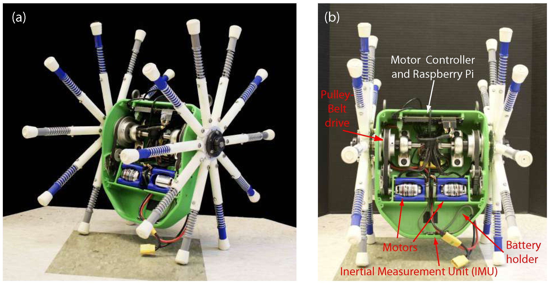
We show the Rowdy Runner 2 (RR2) in Figure 1. The robot comprises two major mechanical components: two sets of rimless wheels (white-colored spokes) placed side-to-side and the torso (green box) in between the wheels.
2.1.1. Rimless Wheels
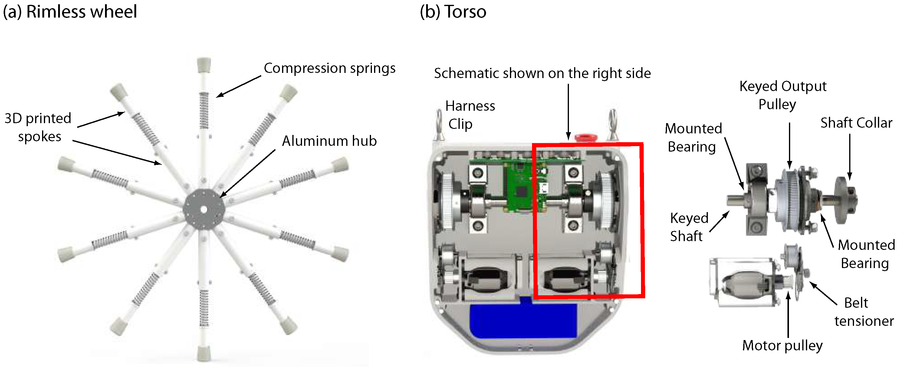
The robot has two sets of rimless wheels; we show one of which in Figure 2a. Each set of wheels has 10 legs, each with a length of 0.26 m. Each leg has four components: a 3D printed tube that attaches to the center hub, an off-the-shelf compression spring, a 3D printed rod that slides into the aforementioned tube, and an off-the-shelf rubber foot. The rod has a lip that contacts the spring and compresses it whenever weight is placed on the leg. A slot designed into the rod allows for constrained movement by securing a screw through the rod and the tube.
All legs connect to a central hub. The hub is one of the highly stressed parts and hence constructed using aluminum. The hub has 10 small cylinders projecting on the outside which are used to secure the 10 tubes of the legs through a screw. These screws prevent the tubes from twisting or falling out. We connect each hub of the rimless wheel to the torso (green box) through a shaft using a keyed shaft collar. We clamp the shaft collar onto the shaft by tightening the key and to provide a secure connection.
2.1.2. Torso
We show the robot torso (green box) in Figure 2b and is 3D printed to allow creating complex geometries such as the bearing alignment holes, circuit board mounts, vent holes, battery compartment, and the motor attachment point.
There are two shafts inside the box that connect to each of the two rimless wheels through a keyed shaft collar. Within the box, each shaft has two mounted bearings; one mounted to the sidewall of the body and one at the end of the shaft inside the body. Having two perpendicularly supported bearings prevents the shaft from moving around from the tension of the belt on the pulleys or during the robot motion.
We securely fasten the two motors to the wall in the body with the faceplate provided by the manufacturer [16]. Each motor transfers power to the corresponding output shaft through two pulleys and a toothed belt with a 5.4:1 reduction. We attach the encoder to the motor with the help of a 3D printed bracket and second output shaft. This bracket holds four nuts that thread the screws coming through the wall and the faceplate. We attach the pulley to the output shaft of the motor with two set screws. We align the motor and the output pulley with each other and rotate them by a GT3 toothed belt. The output shaft is a half-inch keyed shaft that engages onto the output pulley. A shaft collar and sidewall bearing surface hold the pulley in place laterally. We install a small tensioner on the sidewall of the body to stretch the belt and prevent the belt from slipping.
We mount all circuit boards directly onto the torso’s designed standoffs. When mounting directly into 3D printed plastic, the screws can self-tap themselves into the plastic, eliminating the need for a nut. We mount the motor controller and computer to the top of the body using screws into the designed standoffs. The top of the torso has eyelets for a harness, and a cutout for the computer ports. The bottom of the torso holds two batteries and the IMU, the latter of which we mount using four screws.
2.2. Electronics
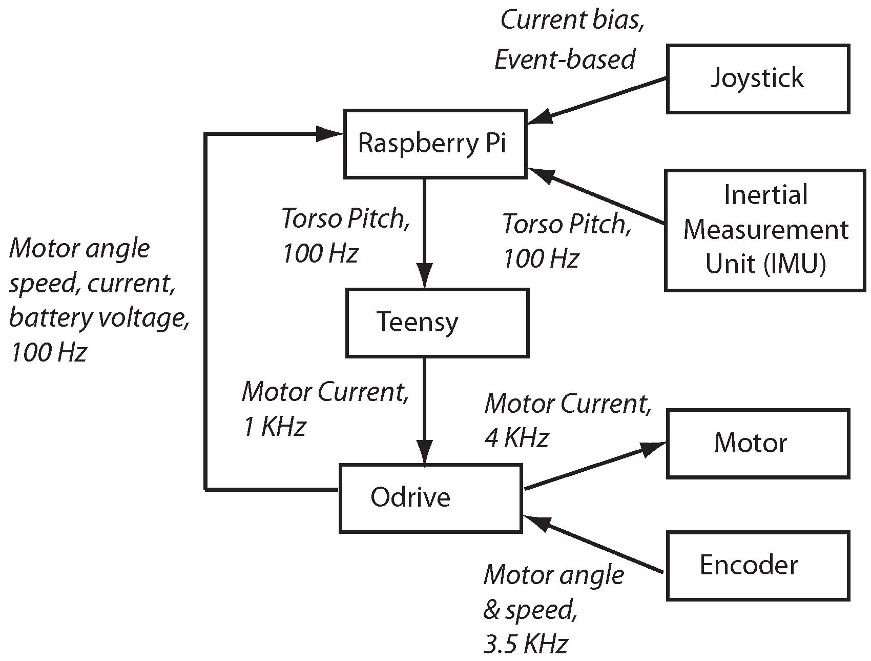
Figure 3 illustrates the electronics used in the RR2 robot. At the highest level is the Raspberry Pi 3B (4 core, 1.2 GHz, 1 GB RAM) that is responsible for system scheduling, reading and storing all sensor data, and relaying data to an external computer. At the middle level is a Teensy 3.2 micro-controller (Cortex-M4, 72 MHz, 64 KB RAM) [17] that uses the body pitch measurement to compute the desired motor current for body torso control. We connect it to the Raspberry Pi through a USB connection. At the lowest level is an Odrive V3.5 [18], a motor controller for brushless direct current (BLDC) motors. We connect the Odrive to the Raspberry Pi through USB and to the Teensy through a serial connection.
The RR2 uses two commercially available BLDC motors with a 280 KV rating [16]. A 280 KV motor will produce 1 V across its terminals if the motor spins at 280 rpm. High KV rating is preferred for high speed and low torque applications, but a low KV rating is preferred for high torque and low-speed applications. We fit each motor with CUI AMT102 quadrature encoder. The Odrive counts the encoder tics and are used to control the BLDC motor. We mount a 9-Degree of Freedom (DOF) orientation sensor BNO055 from Bosch on the torso and is used to measure the torso pitch. We connect this orientation sensor to the Raspberry Pi through a serial connection. The ODrive relays the motor angle, speed, current, and battery voltage to the Raspberry Pi. We use a Dualshock 3 Controller as a remote joystick to control the robot. This joystick has a Bluetooth transmitter, which we pair with the Raspberry Pi. Due to the Raspberry Pi’s mediocre internal WiFi antenna range and performance, we attach a small wireless hotspot to the robot torso for communication and data transfer. We connect this hotspot to the Raspberry Pi through an Ethernet cable, which we power using an USB battery bank (5000 mAh).
We use a 6S 30C 3000 mAh Lithium Polymer (LiPo) battery with a nominal battery voltage of 22.2 V to power the motors. The 30C rating designates that this battery can output a constant current of 90 Amps (A). The 6S rating means that this battery has 6 battery cells in series, totaling the 22.2 V nominal voltage. We use a double cell 3.7V 4000 mAh LiPo battery to power the Raspberry Pi. We connect the battery to a circuit board soldered to the Raspberry Pi that boosts the battery voltage to 5 V and prevents the under-voltage of the battery.
The various electronics communicate at different rates. At the highest level, the Raspberry Pi communicates with the inertial measurement unit, Teensy, and Odrive at 100 Hz. At the middle level, the Teensy communicates with the Odrive at 1 kHz. The Odrive communicates with the encoder at 3.5 kHz and with the motor at 4 kHz. The joystick is an exception that communicates with the Raspberry Pi in an event-driven fashion, i.e., the Raspberry Pi accepts the commands from the joystick only at certain times (e.g., it accepts turning command once-per-step at mid-step).
3. Controller
3.1. Torso Pitch Controller
The goal of the torso pitch controller is to maintain the torso to a set angle to the vertically downward direction. By holding the torso at a set angle during the entirety of motion, it torques the shaft of the rimless wheel. This produces a traction force at the spoke contact that pushes the system forward, thus adding energy into the system. However, the robot loses energy when the legs collide with the ground and friction in the springs and bearings. During the steady-state motion of the rimless wheel, the energy added by the torso equals the energy loss, leading to steady-state speed between steps.
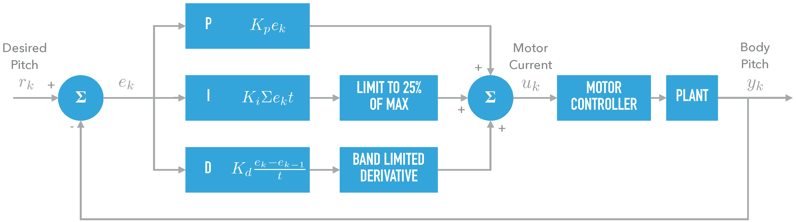
A proportional integral derivative (PID) controller is used to achieve torso pitch control. Figure 4 shows the control diagram of the PID controller. The PID controller at time step k is
where is the current; , , and are the proportional, integral, and derivative gains, respectively, and are all constant during all runs; is the position error and given by the reference pitch angle and the measured pitch angle respectively. We set the reference pitch angle to unless noted otherwise. To prevent integral windup, we limit the integral term () to of the maximum current allowed. The error rate term is noisy, we use an exponential filter to find the filtered error rate . We initialize the filtered error rate to and we tune the constant parameter experimentally. We use .
To tune the PID gains, we place the robot on a table with the legs firmly clamped. We use the heuristics proposed by Wescott [19] as follows: All gains start at zero and we set at an arbitrary number between 0 and 1. The starting value for is , and we increase until we see excessive oscillation or overshoots from the torso. We then reduce the almost unstable by a factor of 2 to ensure a well-behaved gain. Next, we tune by starting with a value between 1 and 100. We tune the gain to where the body oscillates and then fine tune by increasing/decreasing by a factor of 2. Finally, we tune by setting the gain to a value between and . We then fine tune the value using the techniques for the previous gains. Using this method, our tuned gains were A/rad, A/rad-s, and As/rad. An alternate method is to use Ziegler–Nichols method [20].
3.2. Straight-Line Motion
To move straight, both the rimless wheels need to move at the same speed. We achieve this by setting the current in both the motors to the same value. Additionally, the torso angle needs to main a constant pitch angle. We met all these objectives when the motor currents on the left and right are set to be equal to each other and to the constant pitch control given by Equation (1).
3.3. Turning Motion
To turn, we add a differential current to the existing current on one motor and subtracted from the existing current on the other motor.
Since the motor current is proportional to output torque, torque is proportional to the pitch angle, and pitch angle is proportional to the speed we conclude that the motor current is proportional to the robot speed. Thus, the rimless wheel with more motor current will speedup relative to the other side, thus achieving turning. The rationale behind adding/subtracting the same current from the left and right rimless wheel is because the average current in the two motors determines the torso pitch angle, which is still , and thus the torso pitch tries to achieve stabilization at . We set the current differential manually using the joystick.
4. Modeling and Simulation
In this section, we present an overview of the computer model for the rimless wheel. More thorough details are in the supplementary document in Appendix A: Multimedia extension. The computer model has two parts: (a) a steering model based on kinematics adapted from differential drive mobile systems [21], and (b) a sagittal (fore-aft) plane model based on the dynamics [11].
4.1. Steering Model
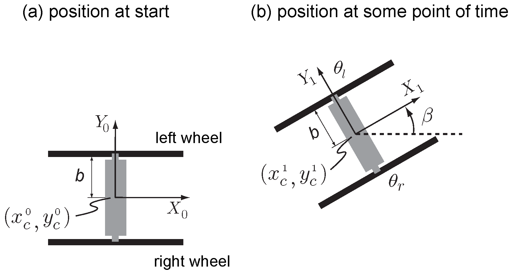
Figure 5 shows the top-down view of the robot as it is turning. The world frame is and the local frame fixed to the robot and moving with it is . In Figure 5a, the local frame coincides with the world frame and in Figure 5b, the robot is at a generic position with the heading angle as shown.
In deriving the steering model, we assume that the relative speed of one rimless wheel relative to the other leads the robot to turn and there are no dynamic effects due to location of the center of mass, which is slightly forward but in between the two rimless wheels. We obtain the kinematics equation for the steering by finding an expression for the linear speed of point C in the local frame, , and and then by relating with the world frame using the heading angle to find the velocity of point C to obtain
where and are the angular speeds of the left and right wheels respectively, ℓ is the length of the virtual leg (defined later in Section 4.2), and b is half the width of the robot as shown. We get the last equation for the heading rate by reasoning about the change in heading as the speed of either sides of the wheel is changed.
4.2. Sagittal or Fore-Aft Plane Model
4.2.1. Equations of Motion for the Stance Phase
We replace the two wheels with a single rimless wheel assumed to be at a point mid-way between the two wheels. This assumption allows the derivation of the sagittal (fore-aft) plane model of the robot and then combine it with the steering model (see Section 4.1) to derive the 3D model for the robot. The center of mass location is in the forward direction and between the two rimless wheels, which is an important consideration in deriving the sagittal model as discussed next.
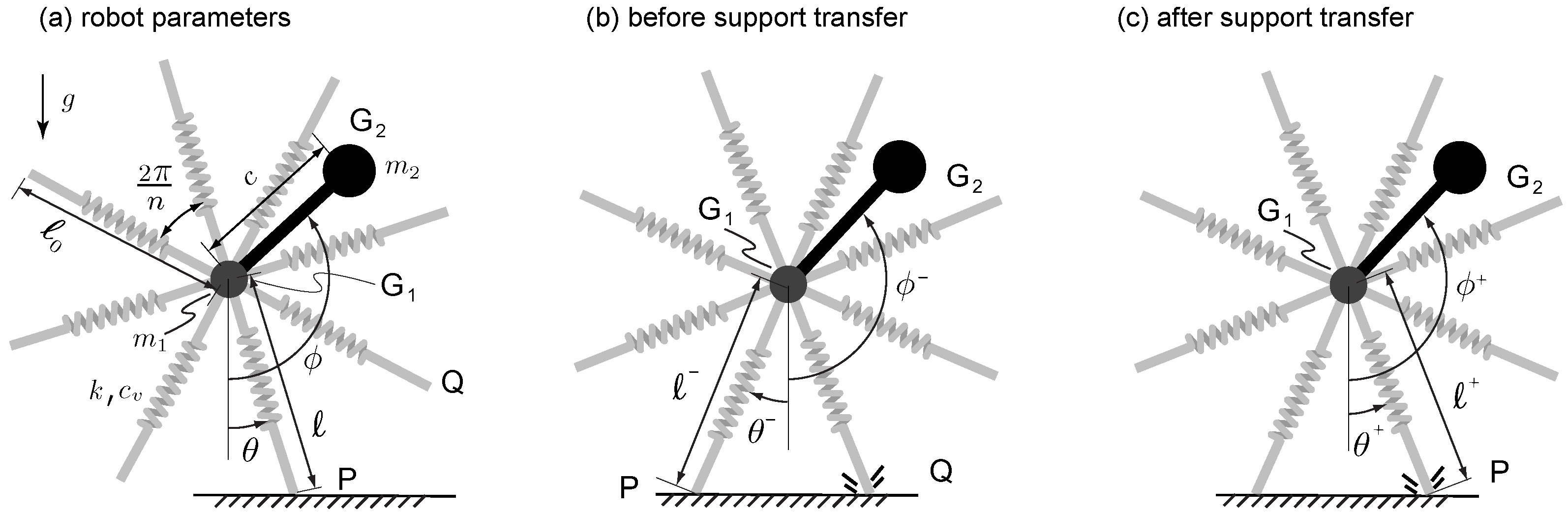
Figure 6a shows the robot parameter and the simulation parameters for the 2D model. This figure is used to derive the equation of motion for the stance phase, which we define as the phase when the two legs on either side of the rimless wheel are touching the ground.
The goal is to find the differential equation for , , , and . We replaced the first two angles with two new angles defined as follows and . Thus, we first find the differential equations for , , , and followed by differential equations for and .
The motor torque at the rimless wheel shaft where produces a traction force at the contacting spoke . For straight motion, the net traction force pushing the robot forward is . For turning, the net moment about the central axis is .
We obtain the equation for from the differential torque and inertia of the robot along the vertical axis as
where and are the motor torques on the left and right wheel, respectively.
We get the equations for , , and by using the principle of angular momentum balance point P and as shown in Figure 6a and principle of linear momentum along the axial direction of the leg on the ground. These three equations are
where , , and are the rate of change of angular momentum about point P, external moment about point P, and external forces respectively, m, , and are the mass, acceleration of the center of mass G, and unit vector along the stance leg, respectively.
From above equations
where , is a 3 × 3 matrix, and is a 3 × 1 vector. Please see the supplementary file for more details in Appendix A: Multimedia extension.
4.2.2. Support Transfer Conditions
To check whether a new spoke has contacted the ground, we need to check the two conditions and which denote the vertical distance between spoke touching the ground (point P in Figure 6b) and the next spoke (point Q in Figure 6b).
The collision condition for the left side wheel and right side wheel are
There are three distinct conditions: (1) legs on either side simultaneously collide with the ground, thus and are both true simultaneously, (2) leg on the left side collides the ground, thus is true, and (3) leg on the right side collides the ground, thus is true.
4.2.3. Equations of Motion for the Support Transfer Phase
During support transfer, there is a hard collision, and the wheel loses energy. We derive th equations for the positions and corresponding rates next. We know the values of the variables before support transfers and we are interested in finding the variables after support transfer, namely .
The assumption made here is that the net difference of velocity before collision is the same as that after collision. This assumption ensures that the two wheels have reasonable speeds after collision. Also note that before and after collision (i.e., during the stance phase), we model the two rimless wheels as a single rimless wheel. Thus
Corresponding to the three collision condition described above, there are three cases: (1) support transfer is through left and right side spokes simultaneously, (2) support transfer is through the left side spoke only, (3) support transfer is through the right side spoke only. We discuss these conditions next.
- (1)
- Support transfer is through left and right side spokes simultaneously
We define the angle as follows
We obtain the equation relating the three degrees of freedom after support transfer to that before support transfer by comparing the configuration of the robot before and after support transfer as shown in Figure 6b,c. These are
where we base the first equation on the fact, the upcoming contacting spoke is unstretched. The angles and are
To find all rates, we define the rate as follows
Next, to find , , and we use the following three equations: the conservation of angular momentum about upcoming collision points Q, conservation of angular momentum about the center , and the conservation of linear momentum along the axial direction
In the Equation (18) we assume that there is no impulsive force along the stance leg. The rationale is that impulse provided by the spring along the radial direction is negligible during the relatively short duration of impact. Combining Equation (18) to get
where , is a 3 × 3 matrix, and is a 3 × 1 vector. Please see the supplementary file for more details in Appendix A: Multimedia extension.
In summary, we obtain the positions from Equations (15) and (16), respectively, and rates from Equations (18) and (20), respectively.
Finally, note that we can find the steering coordinates after support transfer using the positions and rates after support transfer using Equations (5)–(7).
- (2)
- Support transfer is through left side spoke only
- (3)
- Support transfer is through right side spoke only
4.3. Motor Torque and Power Model
The motor torque model relates the torque to the gear ratio G, motor torque constant and current
where for the left and right motor, respectively. The motor power model relates the torque and speed to the power and is given by
The net torque for the simulation is and net power is .
4.4. Computer Simulation
We simulate the system using custom-written script in MATLAB. We need to specify 11 initial conditions: , , , ,, , , , , , and . We integrate the equations of motion given by Equations (8) and (10) using numerical integrator ode113. We use the ‘events’ function in ode113 to detect collision of the spoke with the ground using Equations (11) and (12). Thereafter, depending on the collision type, we use the relevant equations from Section 4.2.2 to relate the positions and rates before collision to that after collision.
5. Results
This section presents the experimental and simulation results. To initialize the robot, we held the robot in a stationary position on two spokes, one on each side. We turn ON the torso pitch controller and allowed to stabilize. Once stabilized, we gently push the robot to impart slight momentum that helps it move forward. For a steady torso pitch angle, the robot achieves a set steady-state speed when initialized in this fashion. To turn the robot, we use a wireless joystick that sets a differential current to each motor as described in Section 5.2.
Our metrics for the robot performance are the overall robot speed, the mean torque on the motors, the power drawn by the motors, the Actuator Cost Of Transport (ACOT) and the Total Cost Of Transport (TCOT). We define the latter two quantities
The difference in ACOT and TCOT is in the power term used in the numerator. The ACOT uses the power of the two motors while TCOT uses the power of the motors and power of the electronics and computers. Thus, TCOT has a greater value than ACOT. A low Cost of Transport (Total or Actuator) demonstrates a more energy-efficient motion.
5.1. Straight-Line Motion
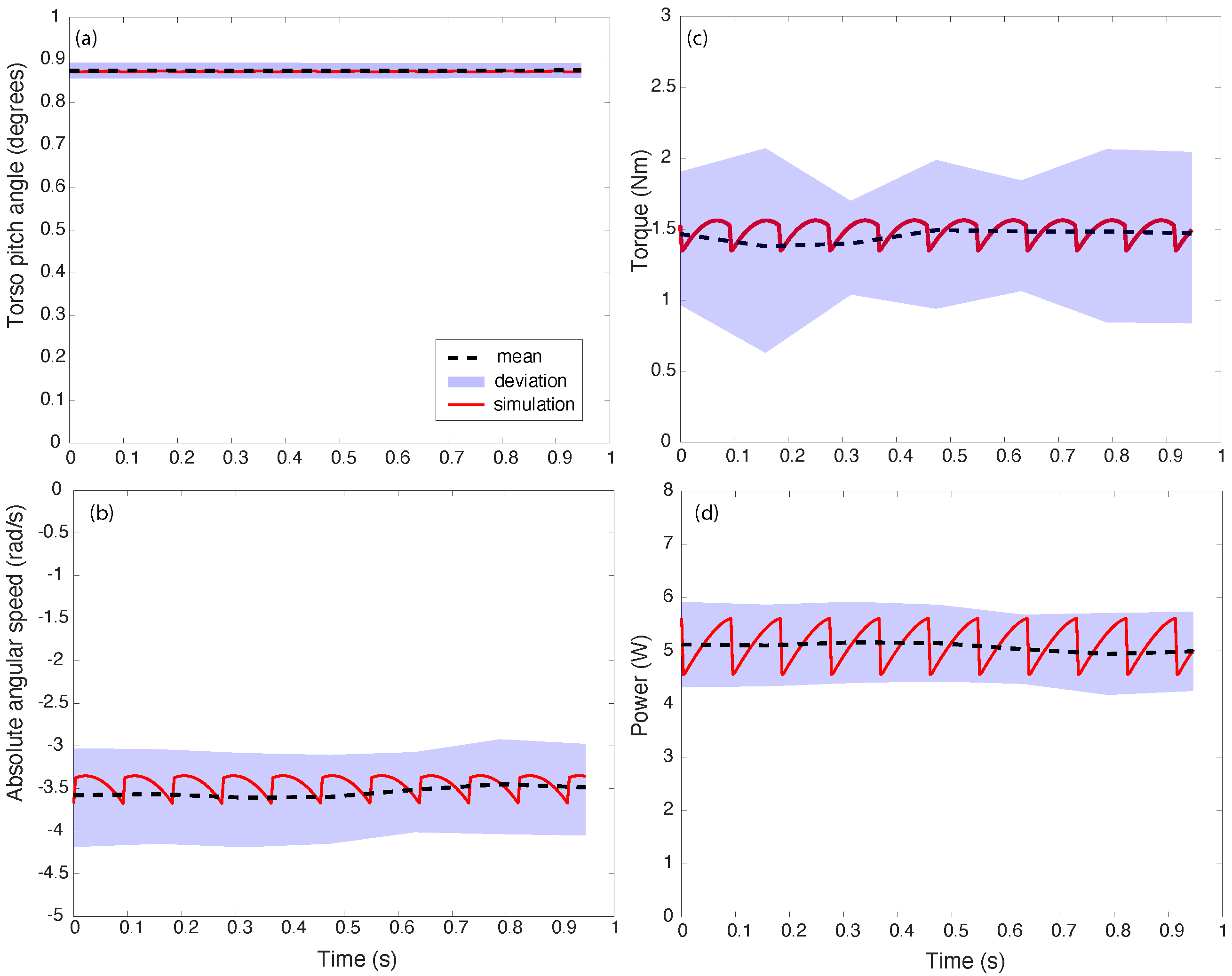
Figure 7 compares the trajectory data between simulation and experiments for a test run on concrete with a torso pitch setpoint of . The data is for 5 seconds after the robot reaches a steady-state speed. The thick red lines are the simulation data, the black dashed lines and blue bands are the mean values and one standard deviation respectively for the experimental data. Although the setpoint tracking is achieved with high accuracy as shown by (a), the speed is within rad/s and the torque is within Nm. The power which is the product of the torque and speed is W. The experimental data is considerably noisy hence the relatively large standard deviation, but the average values between simulation and experiments agree reasonably well as indicted by Table 1. There are two reasons for the spiky data: (1) the collisions during support transfer, and (2) the cogging torque in the motor. The cogging torque is more pronounced when doing a current control as done here. Cogging torque is when there is zero output torque that occurs when the rotor lines onto the dead-band (no magnetic field) of the stator.
We tested the rimless wheel on different surfaces to study the effect of floor compliance on the TCOT and speed. Table 2 shows the results of testing on 5 different surfaces. All these results were for a torso setpoint of and after achieving steady-state motion. As seen from the table, polished concrete has the lowest speed and highest TCOT while asphalt has the highest speed and lowest TCOT.
We also tested the rimless wheel for different torso pitch angle. Theoretically, a torso pitch angle of should give the fastest speed. However, because the torso pitch set-point control is not perfect, the torso would overshoot beyond driving the system unstable. To offset the issue, we limit the torso pitch to a maximum of to the vertically downward direction. The maximum speed achieved with this torso pitch angle is m/s ( mph) on polished wood (i.e., an indoor basketball court).
5.2. Turning Motion
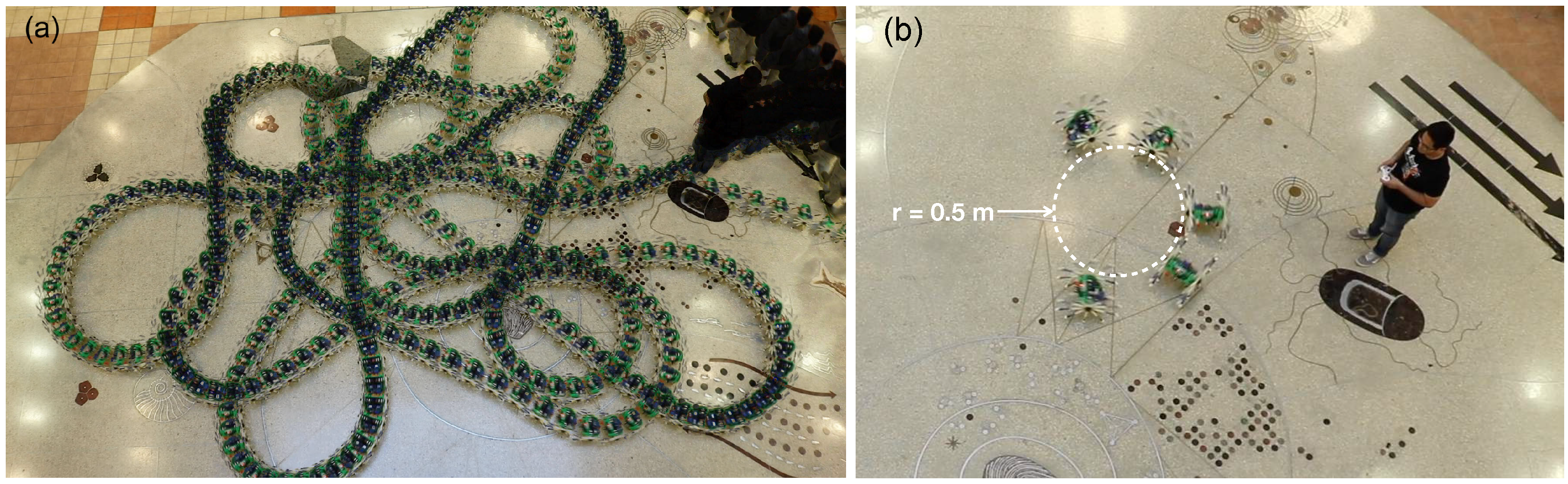
To induce turning, we command the robot torso pitch to and launched to move in a straight line. After the robot reaches a steady-state speed, it turns when commanding different currents in the motors using a hobby remote control. Figure 8a show the path taken by the robot. The robot can turn within the indoor facility without bumping into obstacles. We show the smallest turn radius during our trials in Figure 8b. We obtain the figure by super-posing five video frames and using a calibration scale to measure the radius. The smallest turn radius achieved is m. The turn radius is measured using the inner side of the rimless wheel when it turns. Theoretically the smallest turn radius is zero corresponding to the one wheel stationary and other moving a non-zero speed. The issue is that the torque requirement for this is too low for the robot to hold a constant pitch angle of leading to a loss of forward momentum, consequently coming to a halt. From multiple runs, we found that the robot turns more easily on hard floors at slow speeds most likely because of the better traction between the legs and the floor at slow speeds.
Figure 9 shows the simulation data for turning with a radius of m. Here, the relative difference between the left and right motor current is A. Figure 9a shows the spatial position of the center of the torso as viewed from top. The rimless wheel starts at and turns clockwise. As shown in subsequent figures, the robot takes about s to complete half-turn. The Figure 9b,c shows the torso pitch angle and torso speed. It can be seen that the torso pitch stays around while there is mild fluctuation in the speed. Note that we used a simple position servo without considering the model compensation (e.g., gravity compensation). Figure 9d,e shows the position and speed of the spoke in contact with the ground. It can be seen that the left wheel is traveling faster than the right one. Finally, Figure 9f,g shows the motor torques and motor powers respectively. It can be seen that the differential torque is about 1 Nm and the total motor powers is about W consistent with straight line movement. These results demonstrates that (1) our control algorithm of introducing a small differential current in the two motors is sufficient to get the rimless wheel to turn without losing momentum and (2) validates the kinematics-based steering model.
5.3. Parameter Studies
To do parameter studies, we vary one parameter at a time keeping the other parameters the same as the one for straight-line motion. For each simulation, we start the rimless wheel in the upright position and angular speed rad/s and simulation time is 5 s. The time is sufficiently long for the rimless wheel to achieve steady-state speed. The parameters we vary are the torso pitch angle, location of the center of mass of the torso, the number of spokes, the mass of the wheel, and the stiffness of the springs in the leg.
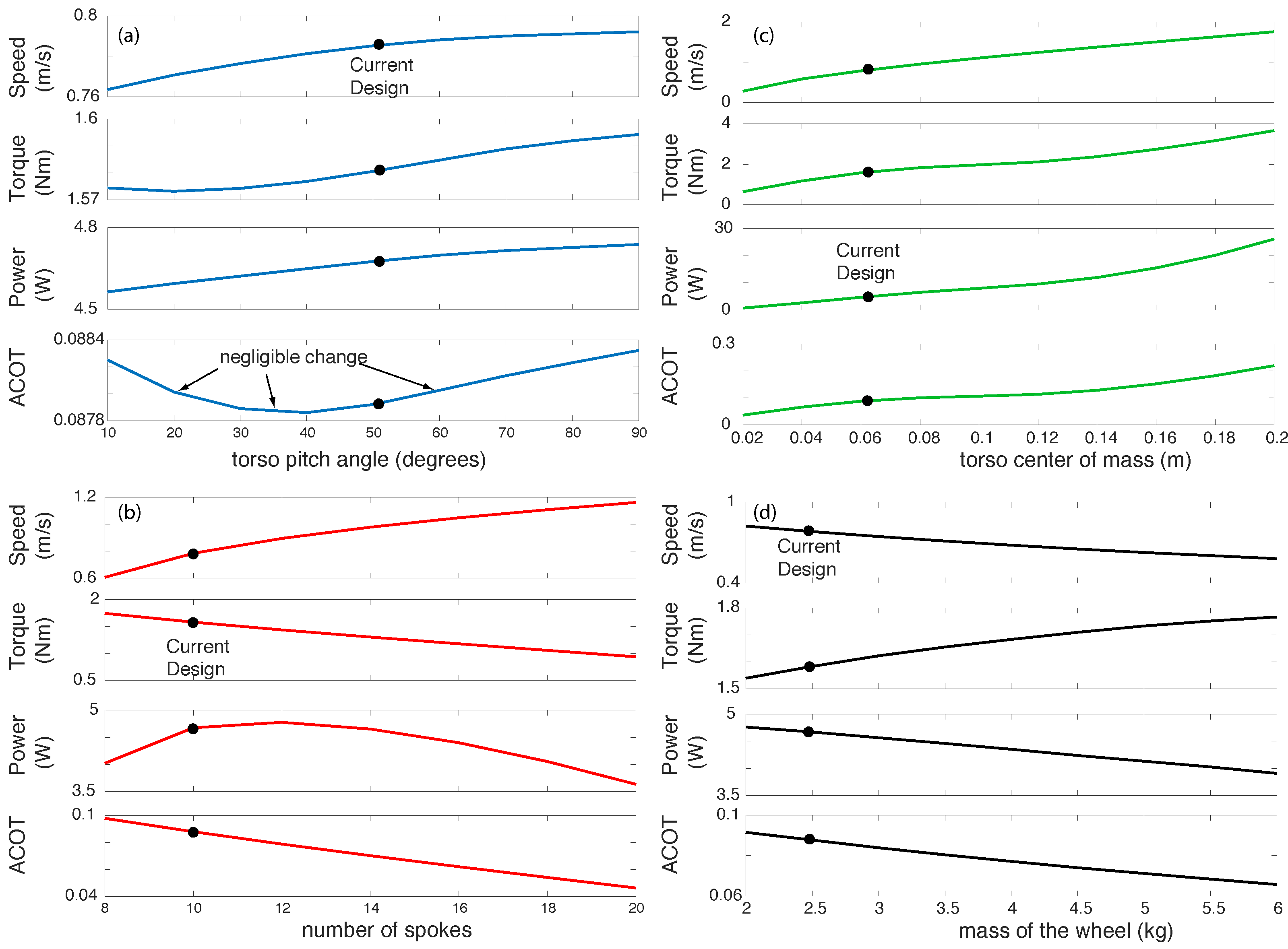
Figure 10 shows plots of the output parameters: average speed, average torque on the torso, average motor power, and average motor cost of transport for all the above parameters except the leg stiffness. We have not shown the leg stiffness data because we found that there are no significant changes in the output parameters when we vary spring stiffness from 500 to 4000 N/m. The black dot in the plot shows the value for the current robot design and the straight-line movement experiment reported earlier. From these plots, we can draw the following conclusions: (1) to increase the speed, the torso pitch angle, the distance of the center of mass from the center of the wheel, and the number of spokes should all increase but the mass of the wheel should decrease; (2) to decrease the torque on the torso, the pitch angle, the torso center of mass, and the mass of the wheel should all decrease but the number of spokes should increase; (3) to decrease power consumption the torso pitch angle, the center of mass location should decrease but the mass of the wheel should increase, but there is a range of spokes between 10 and 12 where the power achieves a maximum; and (4) to decrease the cost of transport, the location of the center of mass from the center of the wheel should decrease but the number of spokes and mass of the wheel should increase, but there is a negligible change as the torso pitch angle changes.
One can use these plots or computer simulations as a starting point to achieve specific performance metrics for the rimless wheel robot.
6. Discussion
This paper presented the design, modeling, and control of a differential drive rimless wheel robot that achieved a maximum speed of m/s ( mph) and a minimum turn radius of m. The kg robot achieved a Total Cost of Transport (power per unit weight per unit speed) between to for different surfaces with speed ranging from to in m/s ( to in mph). The model of the rimless wheel robot comprises a kinematics-based model for steering motion and dynamics-based for sagittal or fore-aft plane for forward movement. The model can explain the energetics, speed, and turning characteristics of the robot. Finally, parameters studies show key parameters that affect the speed and energetics.
The Total Cost Of Transport (TCOT) defined as the power used per unit weight per unit velocity is the most widely accepted measure of energy usage of locomotion [22]. Humans have a TCOT of while walking at a self-selected speed [23]. However, among ‘true’ bipedal robots, the most energy-efficient robots are Cornell biped with TCOT of 0.2 [24] and Cornell Ranger with a TCOT of 0.19 [25,26]. The most energy-efficient legged robot is by ETH Zurich, Cargo at a TCOT of 0.1 [12] while RR 2 at TCOT of 0.13. However, Cargo has large feet and RR2 has multiple spokes. These features afford these robots enhanced stability with no additional controller considerations. The parameter studies the following measures to further decrease the TCOT: (1) moving the center of mass closer to the center of the wheel, thus reducing the motor torque; (2) increasing the number of spokes which leads to lowering the collisional losses; and (3) increasing the total mass presumably because the power increase in the numerator of TCOT is proportionately less than the decrease of TCOT because of the increased mass in the denominator.
The RR2 with 20 total legs reached a maximum speed of 4.3 m/s (9.66 mph). The robot has legs with a length of 0.26 m, which gives it a Froude number of 2.71 (Froude number is where v is speed, g is gravity 9.8 m/s2, and ℓ is leg length). Outrunner, the 0.6 m tall, 6 legged rimless wheel had a Froude number of 5.14 and HexRunner, the 1.83 m tall, 6 legged rimless wheel had a Froude number of 4.82. Thus, RR2 is twice as slow as these other rimless wheels. To increase the speed of the rimless wheel we need to reduce the collisional losses. We can do this either by decreasing its mass or increasing the number of spokes. Alternately one can add more energy to the system during the single stance phase by increasing the pitch angle or increasing the distance of the center of mass from the center of the wheel.
A differential drive-based turning is simple (only two motors needed) and enables a short turn radius. The minimum turning radius achieved by RR2 is 0.5 m (see Figure 8). The low net torque prevents us from achieving the shortest turn radius of 0 m (turning in place) as discussed in Section 5.2. The Outrunner and HexRunner use an oscillating pendulum-like mechanism in the lateral (side-ways) plane for turning, but the minimum turn radius has not been made publicly available. The main difference between RR2 and these runners is that RR2 relies on kinematics to turn (speed of one wheel relative to the other) while the runners rely on the dynamics of the oscillating mass, the location of its center of mass, and oscillating frequency. We need to control the oscillation to ensure that the turning motion does not destabilize the robot in the sideways direction. Although the differential drive rimless wheel and the differential drive wheel have the same turning kinematics, the rimless wheel has hybrid dynamics in the sagittal plane with energy losses during collision, while the wheel has purely kinematic movement without energy losses assuming that it rolls without slipping.
Direct drive motors are attractive because they provide low backlash, low friction, low reflected inertia, mechanical robustness/efficiency, high-actuation bandwidth, and high efficiency [27]. The direct-drive brushless motor used in the robot has a KV rating of 280. This means that for a 1 V voltage output across the motor terminals, the input motor speed is 280 rpm. A high KV ensures high speed but a low KV ensures a high torque. This KV rating did not provide enough torque to support the weight of the torso. Thus we add a pulley transmission to increase the gearing by a factor of , thus increasing the torque without reducing the advantages of the direct drive motors appreciably.
A significant issue with the hobby-grade motors such as the ones used here is the torque ripple or the periodic fluctuation of the output torque for constant input current and load. This is because of the low number of magnetic cores in hobby-grade motors that lead to a lower magnetic strength as the rotor moves from one core to the next. The torque ripple causes controllability issues leading to a poor torque and/or position control (see Figure 7c). The torque ripple made it difficult to achieve rapid modification in the speed and turning.
The rimless wheel had some failure modes. A successful launch was sensitive to the push. Too hard or too slow a push or asymmetrical push leads the rimless wheel to not launch properly causing a failed trial. A fixture for standardizing the launch can solve this issue. On numerous occasions, the rimless wheel ran into walls and broke one or more legs. However, because the legs were modular and 3D printed, it is relatively easy to fix the broken legs.
Rimless wheels are traditionally been argued to be useful in uneven terrain (e.g., sand, rock). However, if rimless wheel can easily move straight and turn, it can be useful in navigating in tight spaces (e.g., warehouses, buildings) such as the case here. In the rimless wheel presented here, we control the speed by maintaining a constant pitch on the torso. Thus, the torso is always at a fixed angle with respect to the world frame. In such settings, one can mount a stereo camera on the torso to enable vision-based movement control.
There are several limitations of the robot that could be addressed in future iterations. The robot cannot self-start and needs to be manually launched. If the robot goes too slow, it comes to a complete stop. This is because there is an energy barrier to cross from the standing position with four spokes (two on each side) touching the ground to the vertical upright position with two spokes touching the ground (one on each side). One way of crossing the energy barrier is by pitching the torso appropriately to pump energy into the wheel. It is challenging to control the pumping with noisy sensors without leading to instability. One option to self-start is to additional means of actuation such as an actuated tail or actuated spokes. The torque ripple prevents high fidelity motion control such as stabilizing against disturbance and quick turning. This issue may be addressed by upgrading to motors with a higher number of magnetic cores [28] or by position or force-based feedback compensation [29]. The robot cannot work on rough terrain such as sandy and muddy terrain and is probably because of its relatively low speed for its size.
Author Contributions
S.S. designed, fabricated, assembled, programmed, and tested the device. P.A.B. did modeling, simulation, and data analysis. S.S. and P.A.B. wrote the manuscript. All authors have read and agreed to the published version of the manuscript.
Funding
The work was partially supported by United States National Science Foundation grants IIS 1566463 and 2010736 to Pranav A. Bhounsule.
Acknowledgments
The authors would like to thank Ezra Ameperosa, Robert Brothers, Panchajanya Karasani, Emiliano Rodriguez, and Ali Zamani for help with testing.
Conflicts of Interest
The authors declare no conflict of interest.
Appendix A
- A video of the hardware prototype available at this YouTube link: https://youtu.be/SNxeP29ayhI (accessed on 15 July 2021).
- Supplementary materials including simulations, animation, mechanical design, and robot code are on github: https://github.com/pab47/RoadRunner2 (accessed on 15 July 2021).
- The MATLAB and Blender code with test examples are on github: https://github.com/EzAme/DR2 (accessed on 15 July 2021).
References
- Margaria, R. Biomechanics and Energetics of Muscular Exercise; Clarendon Press: Oxford, UK, 1976. [Google Scholar]
- McGeer, T. Passive dynamic walking. Int. J. Robot. Res. 1990, 9, 62. [Google Scholar] [CrossRef]
- Bhounsule, P.A. Numerical accuracy of two benchmark models of walking: The rimless spoked wheel and the simplest walker. Dyn. Contin. Discret. Impuls. Syst. Ser. B Appl. Algorithms 2014, 21, 137–148. [Google Scholar]
- Coleman, M.J.; Chatterjee, A.; Ruina, A. Motions of a rimless spoked wheel: A simple three-dimensional system with impacts. Dyn. Stab. Syst. 1997, 12, 139–159. [Google Scholar] [CrossRef]
- Smith, A.C.; Berkemeier, M.D. The motion of a finite-width rimless wheel in 3D. In Proceedings of the 1998 IEEE International Conference on Robotics and Automation (Cat. No. 98CH36146), Leuven, Belgium, 20 May 1998; Volume 3, pp. 2345–2350. [Google Scholar]
- Gomes, M.W.; Ahlin, K. Quiet (nearly collisionless) robotic walking. In Proceedings of the 2015 IEEE International Conference on Robotics and Automation (ICRA), Seattle, WA, USA, 26–30 May 2015; pp. 5761–5766. [Google Scholar]
- Agrawal, S.K.; Yan, J. A three-wheel vehicle with expanding wheels: Differential flatness, trajectory planning, and control. In Proceedings of the 2003 IEEE/RSJ International Conference on Intelligent Robots and Systems (IROS 2003) (Cat. No. 03CH37453), Las Vegas, NV, USA, 27–31 October 2003; Volume 2, pp. 1450–1455. [Google Scholar]
- Laney, D.; Hong, D. Kinematic analysis of a novel rimless wheel with independently actuated spokes. In Proceedings of the 29th ASME Mechanisms and Robotics Conference, Long Beach, CA, 24–28 September 2005. [Google Scholar]
- Cotton, S.; Godowski, J.C.; Payton, N.R.; Vignati, M.; Schmidt-Wetekam, C.; Black, C. Multi-Legged Running Robot. U.S. Patent App. 14/596,514, 7 January 2016. [Google Scholar]
- Isern, W. IHMC Robot Breaks Speed Record. 2019. Available online: https://www.pnj.com/story/news/2014/06/08/ihmc-robot-breaks-speed-record/10211537/ (accessed on 15 July 2021).
- Bhounsule, P.A.; Ameperosa, E.; Miller, S.; Seay, K.; Ulep, R. Dead-beat control of walking for a torso-actuated rimless wheel using an event-based, discrete, linear controller. In Proceedings of the ASME 2016 International Design Engineering Technical Conferences and Computers and Information in Engineering Conference. American Society of Mechanical Engineers, Charlotte, NC, USA, 21–24 August 2016; p. V05AT07A042. [Google Scholar]
- Guenther, F.; Iida, F. Energy-efficient monopod running with a large payload based on open-loop parallel elastic actuation. IEEE Trans. Robot. 2016, 33, 102–113. [Google Scholar] [CrossRef]
- Sirichotiyakul, W.; Satici, A.C.; Sanchez, S.; Bhounsule, P.A. Energetically-optimal Discrete And Continuous Stabilization Of The Rimless Wheel With Torso. In Proceedings of the ASME-International Design Engineering & Technical Conference, Anaheim, CA, USA, 18–21 August 2019. [Google Scholar]
- Sanchez, S.; Bhounsule, P.A. A differential drive rimless wheel that can move straight and turn. In Proceedings of the 2020 IEEE/ASME International Conference on Advanced Intelligent Mechatronics (AIM), Boston, MA, USA, 6–9 July 2020; pp. 514–519. [Google Scholar]
- Bhounsule, P.A. All Files Related to RoadRunner2, a Differential Drive Rimless Wheel. 2020. Available online: https://github.com/pab47/RoadRunner2 (accessed on 15 July 2021).
- Wiegl, O. Dual Shaft Motor D5065 270KV by Odrive Robotics. 2019. Available online: https://odriverobotics.com/shop/odrive-custom-motor-d5065 (accessed on 15 July 2021).
- Stoffregen, P. Teensy USB Development Board. 2019. Available online: https://www.pjrc.com/store/teensy32.html (accessed on 15 July 2021).
- Wiegl, O. Odrive High Performance Motor Control. 2019. Available online: https://odriverobotics.com/shop/odrive-v35 (accessed on 15 July 2021).
- Wescott, T. PID without a PhD. Embed. Syst. Program. 2000, 13, 1–7. [Google Scholar]
- Ziegler, J.G.; Nichols, N.B. Optimum settings for automatic controllers. Trans. ASME 1942, 64, 759–765. [Google Scholar] [CrossRef]
- Siegwart, R.; Nourbakhsh, I.R.; Scaramuzza, D. Introduction to Autonomous Mobile Robots; MIT Press: Cambridge, MA, USA, 2011. [Google Scholar]
- Von Karman, T.; Gabrielli, G. What price speed? Specific power required for propulsion of vehicles. Mech. Eng. 1950, 72, 775–781. [Google Scholar]
- Bobbert, A. Energy expenditure in level and grade walking. J. Appl. Physiol. 1960, 15, 1015–1021. [Google Scholar] [CrossRef]
- Collins, S.; Ruina, A.; Tedrake, R.; Wisse, M. Efficient bipedal robots based on passive-dynamic walkers. Science 2005, 307, 1082. [Google Scholar] [CrossRef] [PubMed] [Green Version]
- Bhounsule, P.A.; Ruina, A. Cornell Ranger: Energy-Optimal Control. Dyn. Walk. 2009. Available online: https://scholar.google.com.hk/scholar?hl=zh-CN&as_sdt=0%2C5&q=Cornell+ranger%3A+Energy-optimal+control.&btnG= (accessed on 15 July 2021).
- Bhounsule, P.A.; Cortell, J.; Grewal, A.; Hendriksen, B.; Karssen, J.D.; Paul, C.; Ruina, A. Low-bandwidth reflex-based control for lower power walking: 65 km on a single battery charge. Int. J. Robot. Res. 2014, 33, 1305–1321. [Google Scholar] [CrossRef]
- Kenneally, G.; De, A.; Koditschek, D.E. Design principles for a family of direct-drive legged robots. IEEE Robot. Autom. Lett. 2016, 1, 900–907. [Google Scholar] [CrossRef] [Green Version]
- Qian, W.; Panda, S.K.; Xu, J.X. Torque ripple minimization in PM synchronous motors using iterative learning control. IEEE Trans. Power Electron. 2004, 19, 272–279. [Google Scholar] [CrossRef]
- Piccoli, M.; Yim, M. Anticogging: Torque ripple suppression, modeling, and parameter selection. Int. J. Robot. Res. 2016, 35, 148–160. [Google Scholar] [CrossRef]
Figure 1.
Robot: (a) Rimless wheel side view and (b) with important components labeled.

Figure 2.
Mechanical Design: (a) A single rimless wheel with compliant spokes, and (b) torso that includes the transmission using belt drives, the motors, the sensors, and the batteries.
Figure 2.
Mechanical Design: (a) A single rimless wheel with compliant spokes, and (b) torso that includes the transmission using belt drives, the motors, the sensors, and the batteries.

Figure 3.
Schematic of the electronics layout: The Raspberry Pi does all the high-level data management including saving the data and receiving inputs from the Odrive motor controller, the inertial measurement unit, and the joystick. The Teensy does the body pitch control using the body pitch data from the Raspberry Pi. The Odrive regulates the motor current based on the input from the Teensy.

Figure 4.
Schematic of the feedback controller: The feedback controller controls the torso pitch using a Proportional-Integral-Derivative (PID) controller at 1000 Hz.
Figure 4.
Schematic of the feedback controller: The feedback controller controls the torso pitch using a Proportional-Integral-Derivative (PID) controller at 1000 Hz.

Figure 5.
Steering model adapted from differential drive systems: A top view of the robot. (a) The world or fixed frame is shown to coincide with robot local frame. (b) The local frame is attached to the robot and moves with it. The steer or heading angles is and the point C is midway between two wheels have the coordinates in the local frame and in the world or fixed frame. For the steering model, a differential equation for the position of C, and heading is found.

Figure 6.
Planar model: The robot is progressing from left to right. (a) The robot parameters used in the simulation, (b) the robot at an instant before support transfer, and (c) the robot at an instant after support transfer. All state variables before and after support transfers are appended a superscript − and + respectively. The point P is the current spoke touching the ground and point Q is the spoke that will touch the ground on the next step. Note that the robot has 10 legs on each side but only 8 spokes are shown in the illustration.

Figure 7.
Experimental data for straight line motion for 1 complete revolution or 10 steps of the rimless wheel: (a) Torso pitch, (b) absolute speed of the robot, (c) motor torque, and (d) power, all as a function of time. The mean is shown with black dashed line and the blue bands show one standard deviation. The simulation data is shown by red solid line. The measurements had considerable noise leading to a relatively large standard deviation.

Figure 8.
Experimental results for robot turning (a) Trajectory of the robot during turning; (b) Shortest turning radius of m.
Figure 8.
Experimental results for robot turning (a) Trajectory of the robot during turning; (b) Shortest turning radius of m.

Figure 9.
Simulation data for turning: (a) Trajectory for circular turn, (b) torso angle, (c) torso velocity, (d) absolute angle of the wheel, (e) absolute angular speed of the wheel, (f) torque on the torso, and (g) total motor power.
Figure 9.
Simulation data for turning: (a) Trajectory for circular turn, (b) torso angle, (c) torso velocity, (d) absolute angle of the wheel, (e) absolute angular speed of the wheel, (f) torque on the torso, and (g) total motor power.

Figure 10.
Parameter studies: Effect on speed, torque, power, and COT for motor as a function of (a) torso pitch angle, (b) number of spokes, (c) torso center of mass, and (d) mass of the wheel. The current design of the rimless wheel is shown by a dot.
Figure 10.
Parameter studies: Effect on speed, torque, power, and COT for motor as a function of (a) torso pitch angle, (b) number of spokes, (c) torso center of mass, and (d) mass of the wheel. The current design of the rimless wheel is shown by a dot.


Table 1.
Comparison of experiment (mean values) on concrete with simulation for torso pitch set-point of .
Table 1.
Comparison of experiment (mean values) on concrete with simulation for torso pitch set-point of .
| Quantity | Experiment | Simulation | |
|---|---|---|---|
| Power | Pi & Sensors | 5 W | |
| Teensy | 0.2 W | ||
| Motors | 5.18 W | 5.17 | |
| Total Power | 10.38 W | 10.37 W | |
| Mean Torque | 1.41 Nm | 1.5 Nm | |
| Mass | 6.9 kg | ||
| Mean Velocity | 0.936 m/s | 0.897 m/s | |
| ACOT (see Equation (25)) | 0.08 | 0.085 | |
| TCOT (see Equation (26)) | 0.164 | 0.171 | |
Table 2.
Cost of Transport and velocities on different surfaces.
| Surface | TCOT | Avg. Velocity (m/s) |
|---|---|---|
| Polished Concrete | 0.16 | 0.936 |
| Polished Wood | 0.15 | 1.197 |
| Indoor Running Track | 0.14 | 1.268 |
| Outdoor Running Track | 0.13 | 1.280 |
| Asphalt | 0.13 | 1.379 |
Publisher’s Note: MDPI stays neutral with regard to jurisdictional claims in published maps and institutional affiliations. |
© 2021 by the authors. Licensee MDPI, Basel, Switzerland. This article is an open access article distributed under the terms and conditions of the Creative Commons Attribution (CC BY) license (https://creativecommons.org/licenses/by/4.0/).
Share and Cite
MDPI and ACS Style
Sanchez, S.; Bhounsule, P.A. Design, Modeling, and Control of a Differential Drive Rimless Wheel That Can Move Straight and Turn. Automation 2021, 2, 98-115. https://0-doi-org.brum.beds.ac.uk/10.3390/automation2030006
AMA Style
Sanchez S, Bhounsule PA. Design, Modeling, and Control of a Differential Drive Rimless Wheel That Can Move Straight and Turn. Automation. 2021; 2(3):98-115. https://0-doi-org.brum.beds.ac.uk/10.3390/automation2030006
Chicago/Turabian StyleSanchez, Sebastian, and Pranav A. Bhounsule. 2021. "Design, Modeling, and Control of a Differential Drive Rimless Wheel That Can Move Straight and Turn" Automation 2, no. 3: 98-115. https://0-doi-org.brum.beds.ac.uk/10.3390/automation2030006