Depolarization Block in the Endocannabinoid System of the Hippocampus


1
Department of Physics, University La Sapienza, 00185 Rome, Italy
2
Via F. Cangiullo, 00142 Rome, Italy
3
Nodes Srl, Via Cornelio Magni, 00147 Rome, Italy
*
Author to whom correspondence should be addressed.
†
Current address: Centro Ricerche, Via Enrico Fermi, 00044 Frascati, Italy.
‡
These authors contributed equally to this work.
NeuroSci 2020, 1(2), 85-97; https://0-doi-org.brum.beds.ac.uk/10.3390/neurosci1020008
Submission received: 3 August 2020
/
Revised: 21 September 2020
/
Accepted: 4 October 2020
/
Published: 24 October 2020
(This article belongs to the Special Issue Feature Papers in Neurosci)
Abstract
:Depolarization block is such a mechanism that the firing activity of a neuronal system is stopped for particular values of the input current. It is important to block epilepsy or unpleasant firing rates. We investigate this property for a non-linear model of CA3 hippocampal neurons under the action of endocannabinoid transmitters. The aim is to discover if they induce depolarization block, a property already seen in other neuronal models and observed in some experiments, signifying that the neural population increases its spiking frequency as some main parameter changes until reaching a situation of no firing. The results is theoretical and it could be useful for investigating real system of neurons of the hippocampus. In some papers it has been shown that this property is connected with bistability, which means that the system has two equilibrium states for some ranges of its parameters. Endocannabinoids influence the learning and memory process and so we concentrate our attention on the CA3 neurons of the hippocampus. We find bistability and depolarization block for the considered model, which is a generalization of the Wilson-Cowan model. The model describes average properties of neurons divided in three classes: the excitatory neuronal population (CA3 neurons) and two types of inhibitory neuron populations (basket cells). The exogenous concentration of cannabinoids is the parameter that controls bistability. This result can be used for an experiment that could give information for medical therapy. We study the time evolution of the synapses connecting the excitatory population with two types of basket cells. The evolution of synaptic weights is considered to be a toy model of the learning process. But this model cannot encompass the complexity and diversity of exogenous and endogenous endocannabinoids effects in vivo.
Keywords:
bifurcation theory; ordinary differential equations second order; depolarization block; synaptic weights; learning process; CA3 neuronsPACS:
02.30 Oz; 02.30 HqMSC:
92B20; 92B051. Introduction
Learning and memorization are regulated at the synaptic level by chemical substances termed neurotransmitters. Amongst those, endocannabinoids displays a peculiar biological behavior. The endocannabinoids are part of the wider cannabinoid (CBs) family of neurotransmitters, which includes:
- Phyto-CBs, they occur in flowering plants, liverworths and fungi. They were first isolated from Cannabis sativa L., more thant 113 different cannabinoids were classified into distinct types: cannabigerols (CBGs), cannabichromenes (CBCs), cannabidiols (CBDs), (-)--trans- tetrahydrocannabinols (-THCs), (-)--trans-tetrahydrocannabinols (-THCs), cannabicyclols (CBLs), cannabielsoins (CBEs), cannabinols (CBNs), cannabinodiols (CBNDs), cannabitriols (CBTs), and miscellaneus cannabinoids;
- Synthetic-CBs (produced in the laboratory);
- Endocannabidoids (eCBs), naturally produced by the human body.
The phyto-CBs and the synthetic CBs can be grouped in the category of exogenous cannabinoids to be distinguished from the endogenous cannabinoids.
The widespread interest in endocannabinoids is motivated by recent experimental studies indicating that these neurotransmitters have an important modulatory action towards both excitatory and inhibitory neurons [1].
Cannabinoids are an example of retrograde messengers that are produced by the post-synaptic cells under certain conditions in order to engage their receptors on the pre-synaptic cell. The activation of these receptors (termed receptors) triggers a reduction in secretion of the neurotransmitter , which is responsible for the inhibitory activity of the pre-synaptic cell on the post-synaptic cell [2,3]. Therefore this mechanism by inhibiting release generates a phenomenon known as Depolarization-Induced Suppression of Inhibition (DSI) [4]. The reduction of inhibitory activity allows storing of information deriving from both internal (sent from body to brain) and external stimuli.
It is thus generally believed that endocannabinoids are able to affect learning and memorization because of their ability to regulate the potentiation of synaptic connections. In particular, it has been shown that damage of the cannabinoid system (that can be caused by exogenous cannabinoids or by schizophrenia or other mental illnesses) can negatively influence learning and memorization [5,6]. It is thus important to understand how cannabinoids affect neuronal activity. The exogenous cannabinoids bind to the same receptors as endocannabinoids and are thus able to alter the natural function of these neurotransmitters. Utilizing the Zachariou et al. [6] model (the relevant equations are described in Section 4), one can analyze qualitatively these phenomena by modifying the exogenous cannabinoids concentration. This model describes the effect of cannabinoids on the pyramidal neurons and on the basket cells along the perforant pathway. The model considers the evolution of the populations of three types of neurons: neurons and basket cells with inhibitory action on the neurons, the basket cells of type A having fast activity and those of type B being with slow activity We study the learning process in the sense that we look for the evolution of the synaptic weights connecting the excitatory populations of neurons with these two different types of basket cells. We notice also that there is no experimental evidence of the influence of exogenous cannabinoids on the occurrence of the depolarization block, while it is evident that exogenous cannabinoids influence the learning process. The simulation of the learning process is given by the dynamics of the synaptic weights connecting the excitatory population of neurons with the slow and fast basket cells. The learning process is modulated by varying both the external and the internal cannabinoids concentrations. The equations utilized in this study are based on the Wilson and Cowan model [7], to which the endocannabinoids dynamics is added. In particular, we analyze the bifurcations of the model in relation to the variation of the exogenous endocannabinoid concentration and, subsequently, we focus on the depolarization block. This important phenomenon has been discussed by Bianchi et al. in relation to the CA1 neuronal pathway [8]. We also show the connection of depolarization block with bistability. This connection has been established in a paper by Kutznetzov et al. [9]. The dynamical model employs variable synaptic weights in time, so we study at the same time the memorization process of the system of CA3 neurons of the hippocampus. This concept has been introduced by the Canadian psychologist Donald Hebb [10], who postulated in 1949: "When an axon of cell A is near enough to excite cell B repeatedly or consistently takes place in firing it, some growth process or metabolic change takes place in one or both cells such that A’s efficiency, as one of the cells firing B, is increased", placing this mechanism at the basis of learning and memory. Some highly relevant studies on the functional architecture of the hippocampus and its role in learning and memory can be found in [11,12,13,14,15]. In Section 2 we find all the bifurcations, stability of limit cycles, saddle node bifurcations of cycles. In Section 3 we discuss the results and give an interpretation in neurobiological terms of these mathematical properties.
2. Results
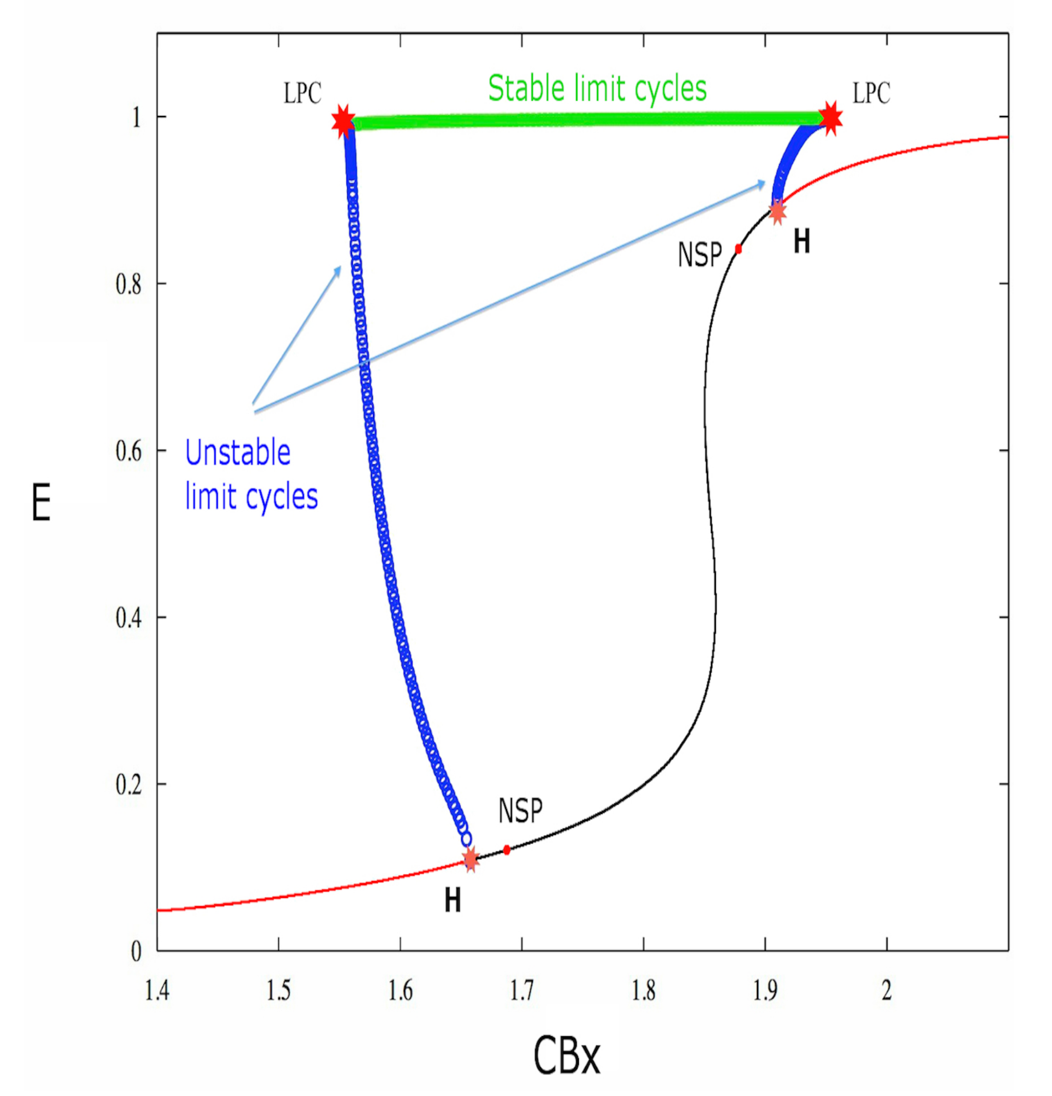
The equilibrium point utilized for the system bifurcation study is obtained by setting the exogenous cannabinoid concentration and the applied external current I equal to zero. Since the model used by us concerns the behavior of neuronal populations, all the results are about the collective behavior of the excitatory neurons. Thus equilibrium points, stability, cycles, are properties of the group of neurons of the same type, and we suppose that the majority of the neurons have the property of the group in the real dynamics. The bifurcations are subsequently studied by modifying the exogenous cannabinoid concentration. Figure 1 shows the obtained chart (the x axis represents the exogenous cannabinoid level and the y axis represents the excitatory activity of the main neuronal population E).
As shown in Figure 1, the system is characterized by two Hopf bifurcations, and two Neutral-Saddle points for certain values of the model parameters reported in Table 1. The Neutral-Saddle is a point (precisely a saddle point) such that the two real eigenvalues are equal in module.
The first Lyapunov coefficient is positive for both Hopf bifurcations (cf. Table 1), therefore these bifurcations are subcritical. Indeed, Figure 1 shows that, for the first bifurcation point, the stable equilibrium (red curve) becomes unstable (black curve). Furthermore, unstable limit cycles (blue circles) also appear. The unstable limit cycles collide as the parameter increases, through a saddle-node bifurcation of cycles (LPC), with stable limit cycles (cf. Figure 1 and Figure 2).
The saddle-node bifurcation of cycles is analogous to the saddle-node bifurcation for equilibrium points. So in a saddle-node bifurcation of cycles, two limit cycles, one stable and one unstable, approach each other until they collide and disappear.
In order to analyze the effect of the reduction of inhibition and increase of excitation, the first factor is more important than the second, therefore one has to study the frequency of the neuronal emission of spikes in the presence of limit cycles.
Figure 3 shows (left to right) that up to the value of the frequency of both stable and unstable limit cycles increases with increasing values of . There is only a small interval, near to the saddle-node bifurcation of limit cycles, where this type of behavior is inverted for unstable cycles. At the frequency decreases, because the system has a second subcritical Hopf bifurcation. This can be explained physiologically by the observation that a strong stimulus can force the neuron transmembrane potential in a depolarized state of equilibrium, preventing the neurons to emit spikes. In general Hopf bifurcations, both subcritical and supercritical, can terminate the periodic activity of the neuronal dynamics.
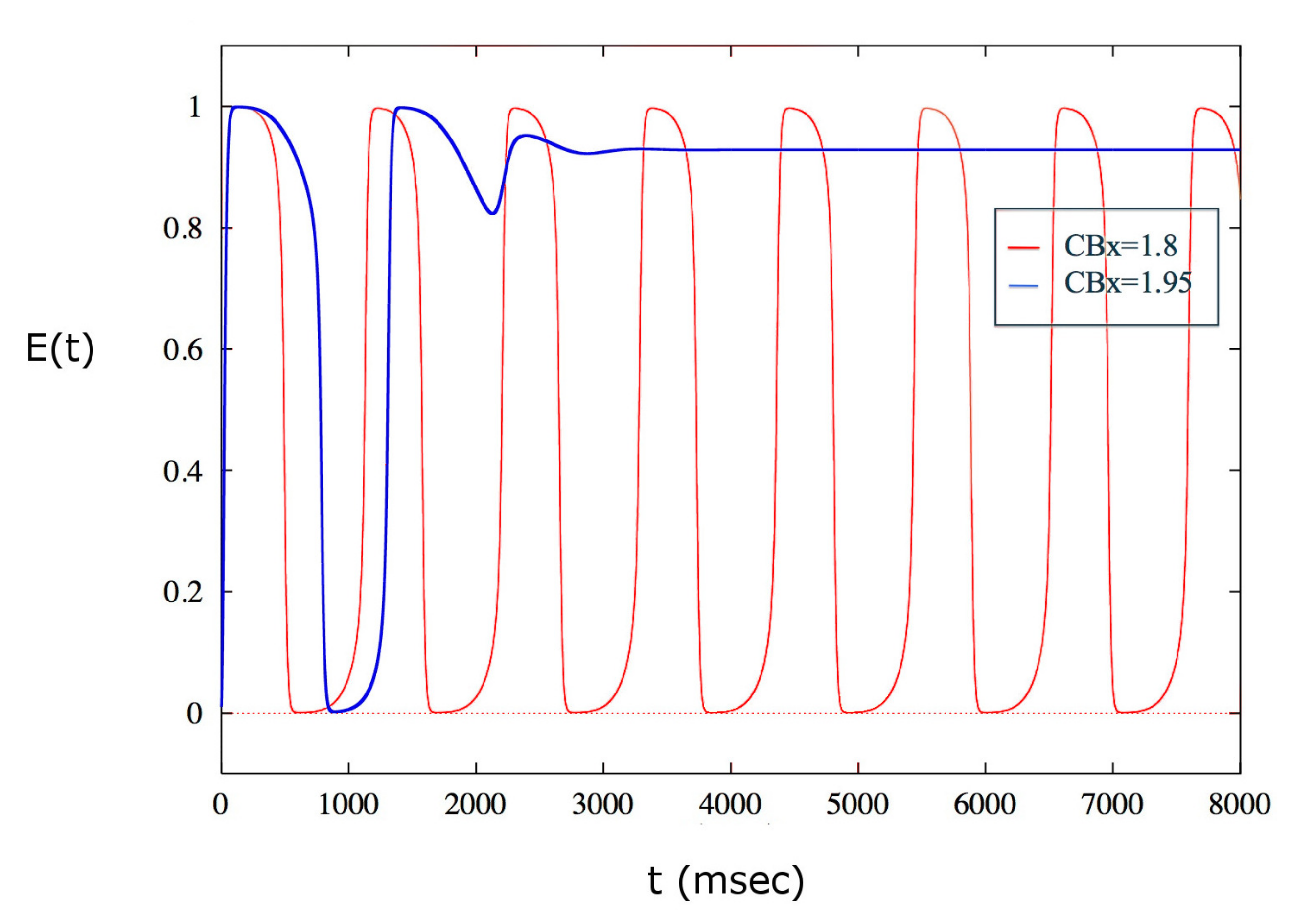
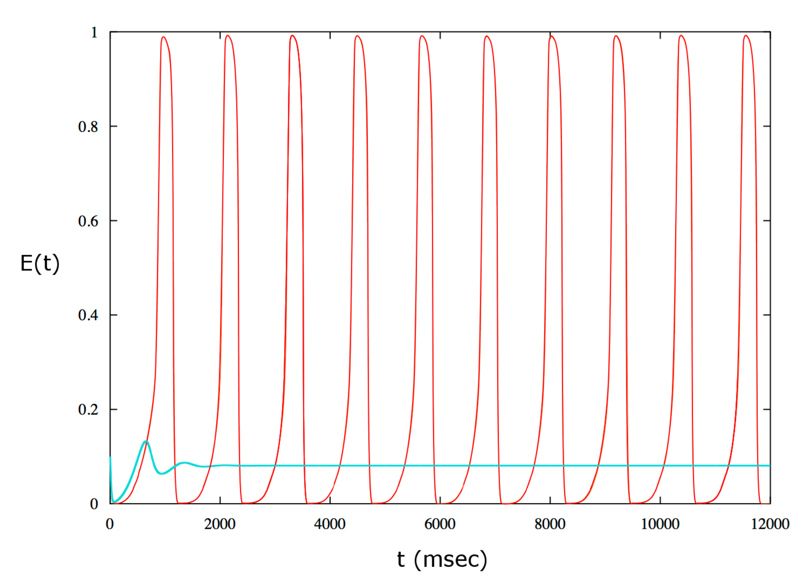
The behavior of the solutions of the model allows us to hypothesize the presence of a depolarization block for a certain value of exogenous cannabinoids higher than . By performing several simulations, it is possible to determine a critical value of , , such that has a depolarization block, i.e. the spiking activity of the population of neurons ceases. The population remains silent for all values larger than this critical value. This behavior is illustrated in Figure 4.
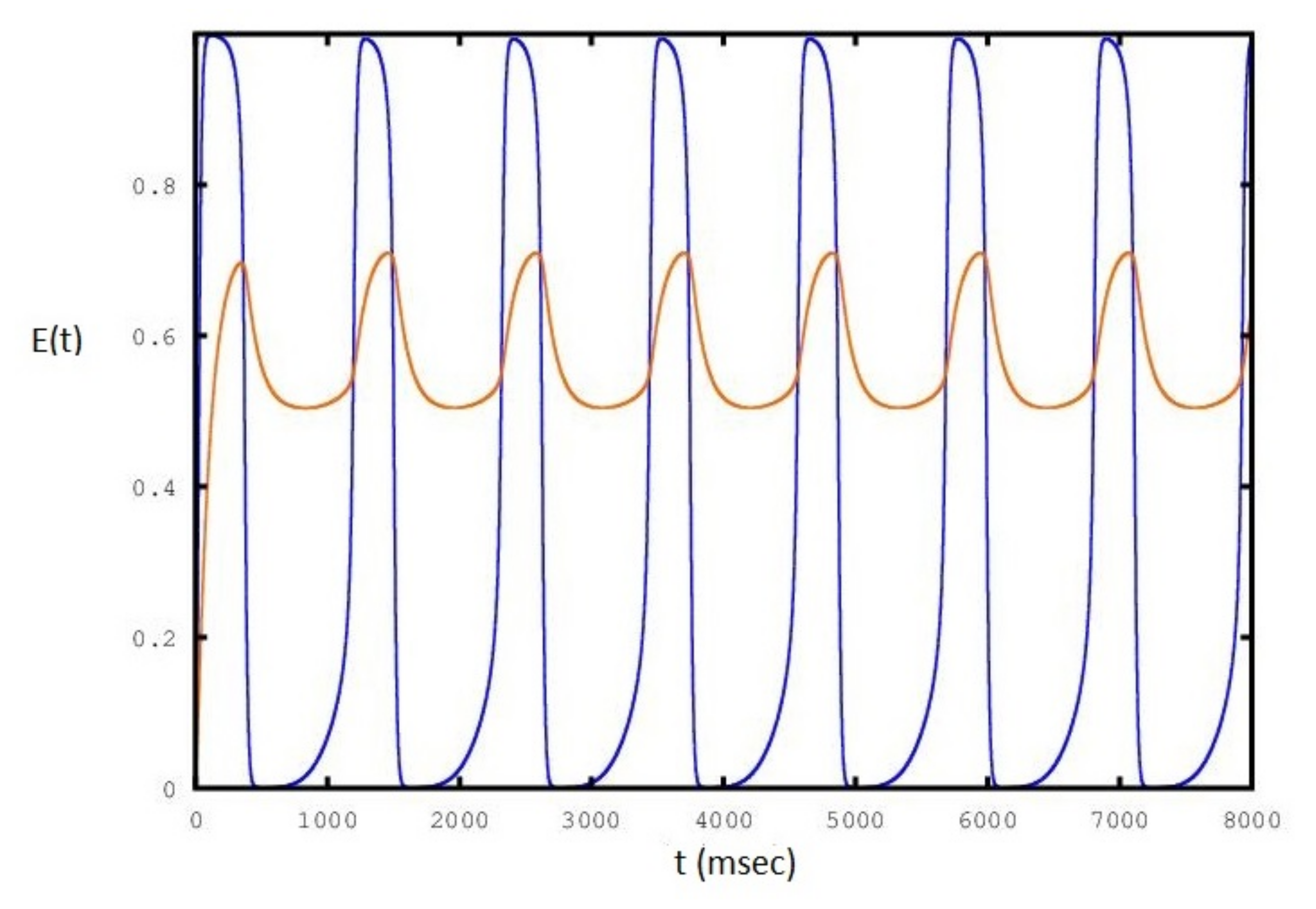
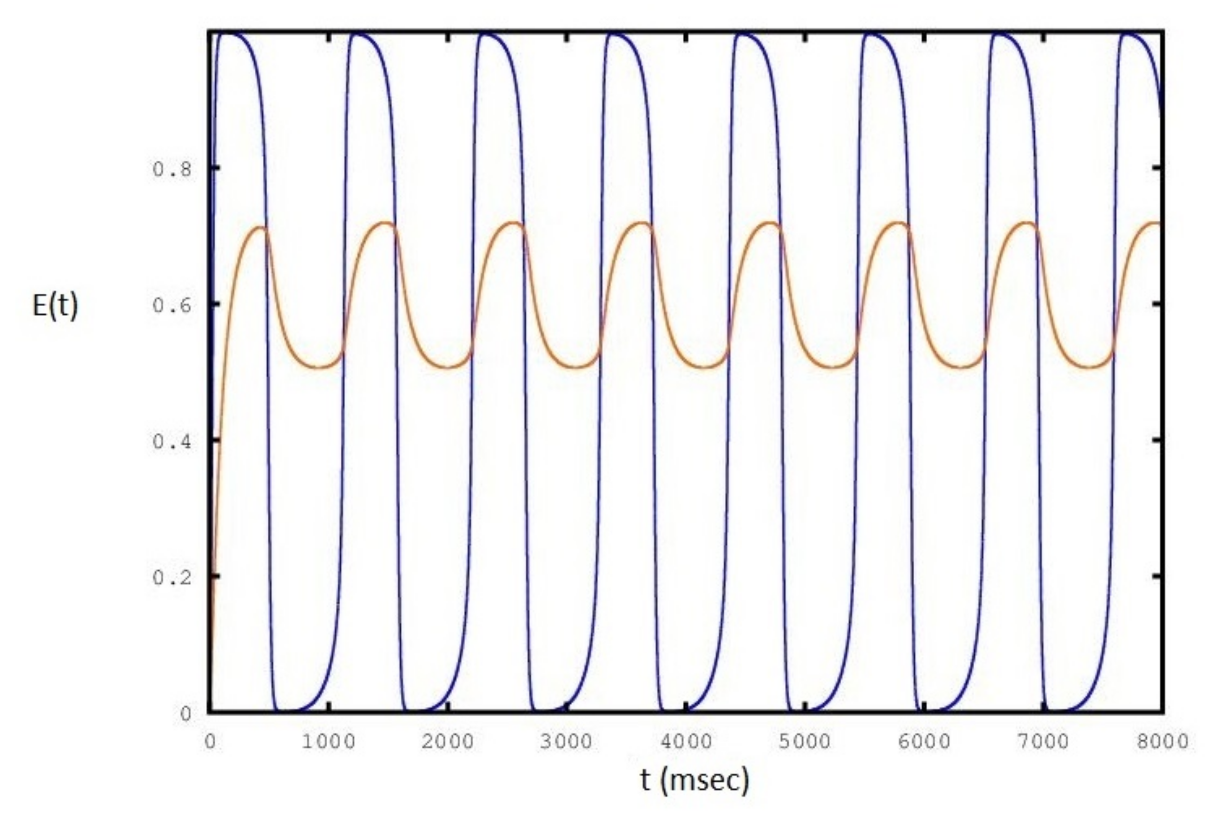
We show in Figure 5, Figure 6 and Figure 7 the sequence of stable cycles of the collective behavior of the E neural population for different values of the parameter. The frequency has the same behavior as in Figure 3: it increases and decreases at the end of the interval and has a maximum in the middle of the interval.
It is interesting to determine whether the depolarization block occurs in the bistability range. The saddle-node cycle bifurcation is obtained for a value of smaller than the one generating the Hopf bifurcation. Therefore in the region between the saddle-node bifurcation of cycles and the subcritical Hopf bifurcation there are two simultaneous stable solutions: the equilibrium point and the periodic solution. In this situation, termed bistability, the neuron can either be quiescent or in an active state of periodic spike emission for a certain depending on the initial state of the dynamics (see Figure 8).
Varying the bifurcation parameter in Figure 1 from right to left, one can see the same behavior for the second Hopf bifurcation point. As we can see in Table 1 and Figure 1, the values of exogenous cannabinoid concentation for which one has bistability belong to the intervals
Therefore the critical value for which we have the depolarization block belongs to the bistability interval.
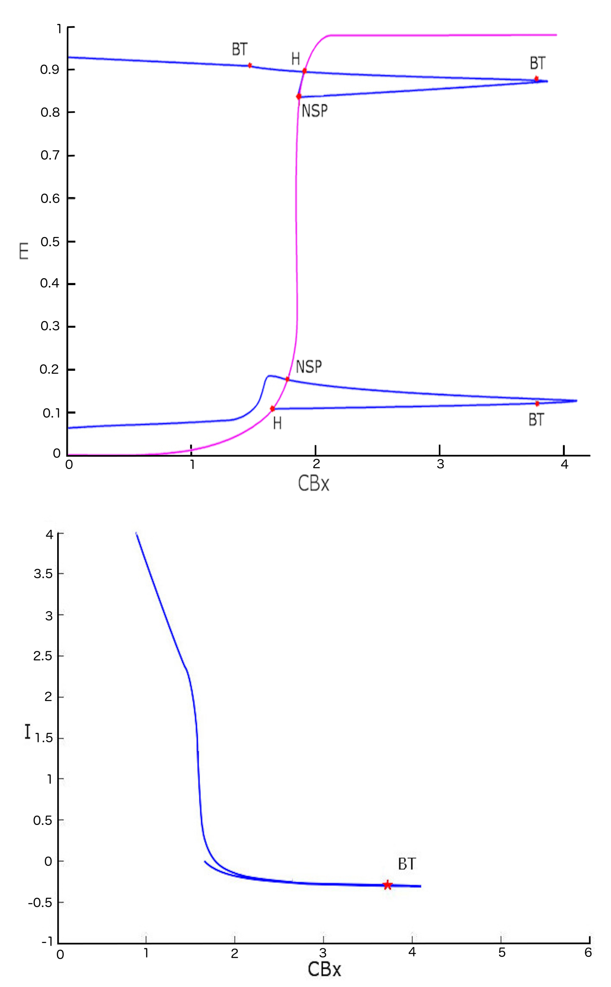
We can show that there are various bifurcations in two-parameter space. Studying the diagram of the first and second Hopf point including the variation of the external current I as well, we obtain the bifurcations reported in Figure 9.
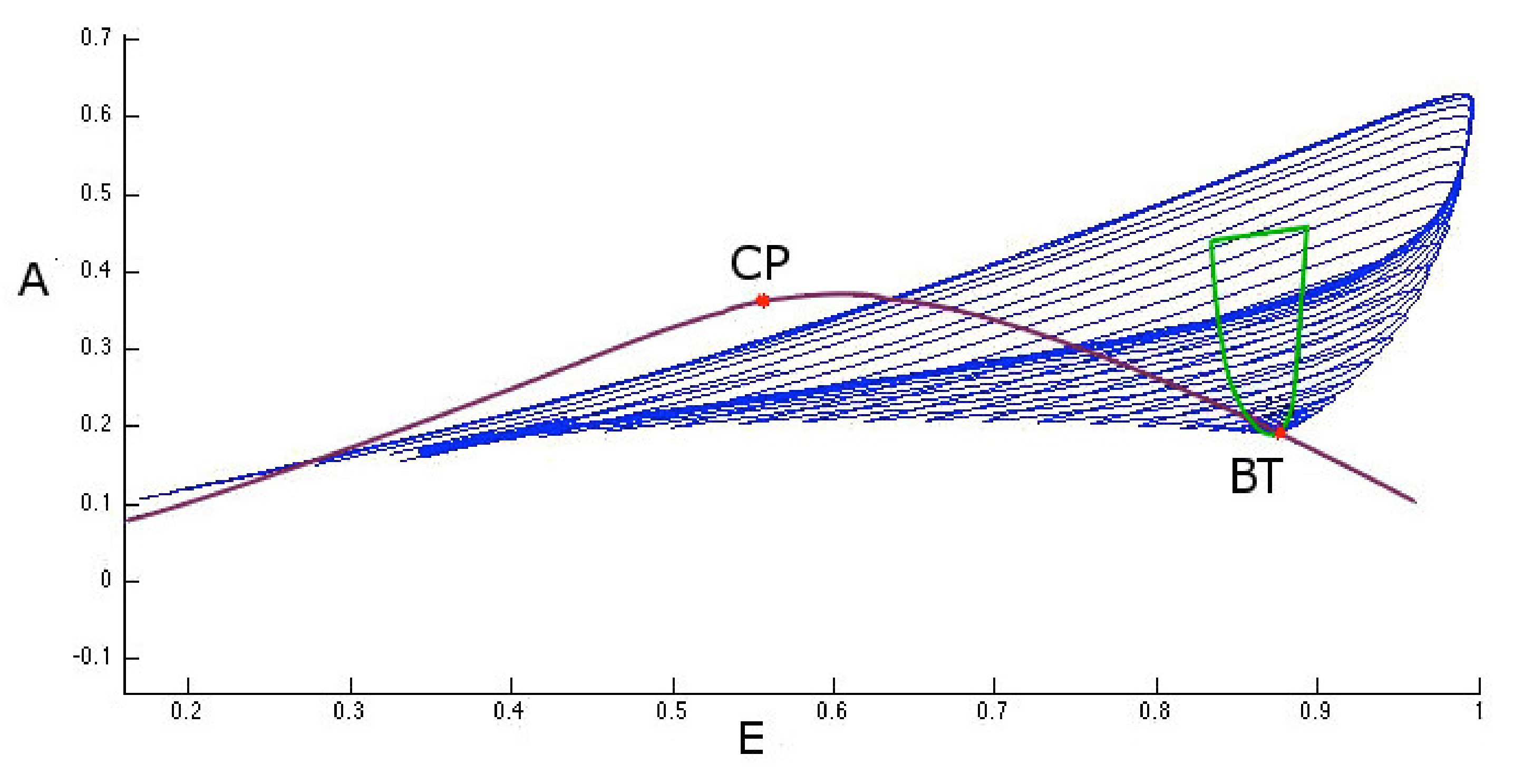
The first point of bifurcation we observe is Bogdanov-Takens (BT) ( the case when the two eigenvalues are equal to zero). The presence of such a bifurcation allows us to postulate the existence of a saddle-node bifurcation for a fixed I value. Bogdanov-Takens bifurcation is obtained when the saddle-node bifurcation collides with an Andronov-Hopf bifurcation. As shown in Figure 10, the BT bifurcation originates exactly in the intersection point of the two curves represented by the Hopf diagram (green) and the saddle-node bifurcation diagram (violet).
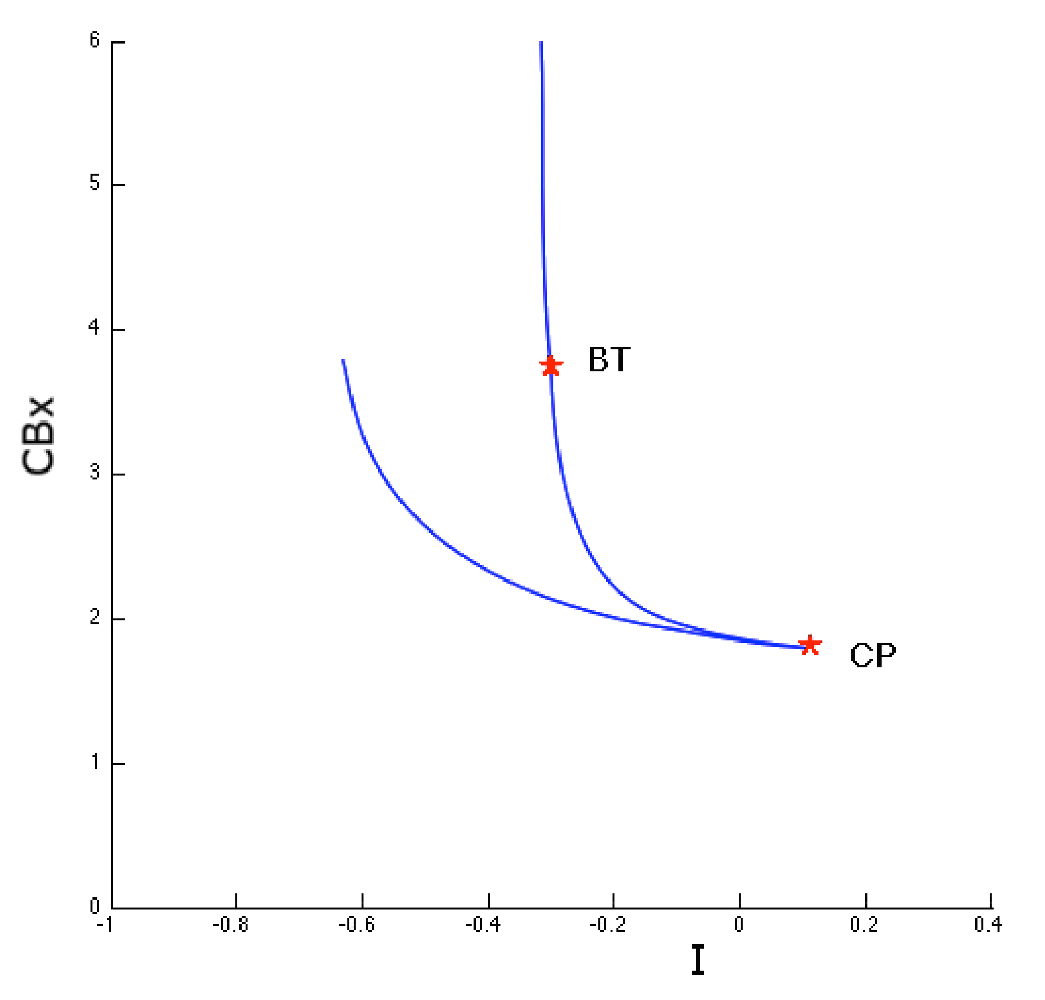
Figure 10 also shows another type of two parameter bifurcation: the cuspid (indicated with the CP label). The cuspid is a two-parameter bifurcation that can be found in an autonomous differential equations system, and is generated when two saddle-node bifurcations collide. Thus, this bifurcation type is seen when, in the two-parameter space, two branches of the saddle-node bifurcation diagram touch each other tangentially originating a semicubic parabola. In fact, if we analyze the area surrounding the cuspid point shown in Figure 10 (in the plane with I and coordinates) we obtain the semi-cubic parabola as shown in Figure 11.
For parameter values close to that of cuspid bifurcation, the system can present therefore three types of equilibrium that disappear in a single saddle-node bifurcation.
3. Discussion
The two subcritical Hopf bifurcations that have been found in this study have a precise neurobiological meaning. For each of the two bifurcations there is a stable fixed point surrounded by an unstable periodic orbit. Instability in this case means that if one looks for the periodic orbit in the space, any small departure from it will bring the system of CA3 neurons out of this periodic orbit. An unstable limit cycle (similar to an unstable node or focus) means that the dynamic system intrinsically departs from it and falls either in a stable node or a stable limit cycle. Thus it is very difficult to reveal it during the simulation. When the parameter approaches the critical value, which is in the interval for the first transition and in the interval for the second transition, the unstable periodic orbit collapses on the stable point which becomes unstable. The main effect is the change of stability of the equilibrium point of the neuron population.So for every value of the main parameter ata the left of the first H point in Figure 1 there is an unstable periodic orbit, and another unstable periodic orbit appears after the second H point. These cycles are important but rather difficult to catch numerically. The two Neutral Saddle Points (NSP) in the figure are two fixed points in the limiting case when the two eigenvalues are equal. The saddle point is a point which is stable in one eigenvalue direction and unstable in the other one, meaning that one eigenvalue is positive and the other is negative. So a saddle point is an unstable equilibrium point: in the special NSP case the two eigenvalues have equal absolute value. This means that a small perturbation of this motion in the stable direction should amplify the motion in a similar way as the perturbation in the other direction. The saddle-node bifurcation of the cycles (or limit point of cycles - LPC) is the analogous of the saddle-node bifurcation of equilibrium points. An unstable orbit collides with a stable one and they annihilate each other: in the case of equilibrium points a stable one approaches an unstable one and disappears. In terms of neuronal oscillations this means that there are two oscillations of the CA3 excitatory neurons, one stable and another one unstable, which approach each other and disappear for the values of shown in the picture. There is also a line of stable limit cycles connecting the two LPC cycles. These are stable oscillations of the E population of neurons. The set of stable cycles corresponding to the green line of Figure 3 is shown in Figure 5, Figure 6 and Figure 7: the frequency changes in agreement with Figure 3. In general these geometrical figures have a basin of attraction, so not all the LPC, NSP, unstable or stable orbits have been found during this study but the knowledge of their existence gives an indication for what values of parameters one can have such a behavior of the system. In order to see all of them it is necessary to choose in a proper way the initial conditions, which represents a lengthy and tedious work. We also underline that the behavior with respect to the parameter is not changed if one varies the b parameter of the endocannabinoids or the parameters of the sigmoid function used in the main evolution Equation (1). The other type of Hopf bifurcation is the supercritical one, which does not appear for this model. From the theory of stability of solutions of systems of differential equations it is well known that the sign of the Lyapunov coefficient determines the type of Hopf bifurcation. In our case these coefficients are both positive and so the transition is subcritical. The concept of bistability is explained in the section of the Results. We want to mention here that it is clear from Figure 4 that there is a block of the spiking activity of the E population, and from Figure 5, Figure 6 and Figure 7 that when approaches the first Hopf bifurcation point the spiking frequency increases (, and are the values of the parameter) and then for the spikes vanish. In these figures is reported and one can see that it oscillates with the activity of the group of the excitatory population of neurons. This implies the oscillation of the synaptic coupling weights and so there is a learning process going on, which ends when the oscillations cease. The meaning of the phase diagram obtained by varying two parameters is more subtle but it can be analyzed in an analogous way. The model we used is a simplified mathematical model, it is intrinsically limited and cannot encompass the complexity and diversity of the effect of exogenous and endogenous endocannabinoids in vivo [16]. The main effect of endocannabinoids on synaptic plasticity is long-term depression (LTD) (not long-term potentiation), first observed in the striatum [17] and then in other brain structures [1]. Furthermore smoking cannabis impairs short-term memory [18]. Mice treated with tetrahydrocannabinol (THC) show suppression of long-term potentiation in the hippocampus [19].
4. Materials and Methods
The model used in this article is taken from [6] and is based on the Wilson-Cowan model. The Wilson-Cowan (WC) [7] model consists of two nonlinear first order differential equations, created to describe the dynamics of a neuronal population, localized in space, containing both excitatory and inhibitory cells. This model describes the averaged dynamics of a class of neurons and thus is not a model of individual neurons. Nevertheless we consider it interesting also because the single neuron model cannot be studied with bifurcation analysis due its complicated phenomenological structure [4]. In contrast to the Wilson and Cowan model [7], in this model we utilize three differential equations describing the activity of excitatory synapses, of the inhibitory synapses (characterized by a slow action) and inhibitory synapses (characterized by a more rapid action).
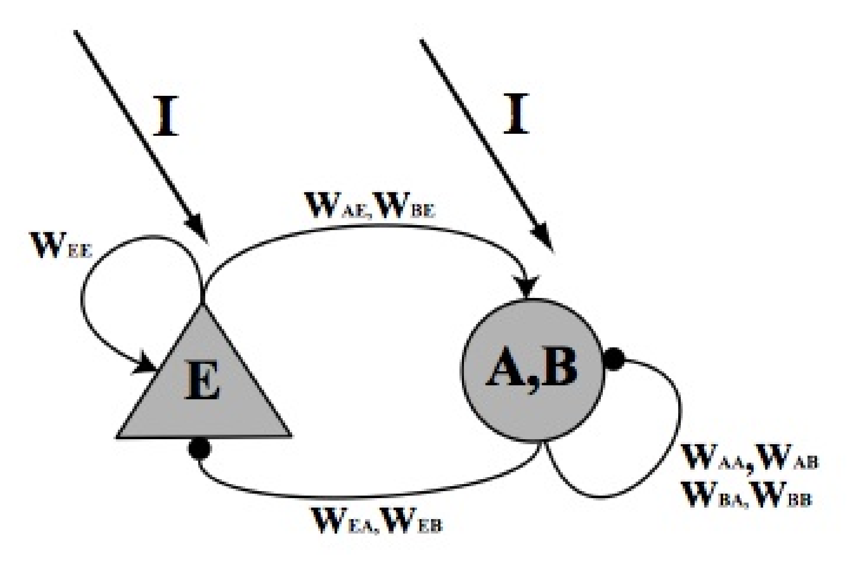
The cells utilized in this model are the pyramidal cells, representing the excitatory population, and the basket cells, representing the inhibitory population. Both types of cells are constituent part of the CA3 hippocampal pathway. In Figure 12 the scheme of the model is represented.
The activity of the cells is described by the following equations:
where
with parameter. The variable E represents the activity of excitatory population while the variables A and B are the fast and the slow interneurons activity respectively.
Another difference between this model and the Wilson and Cowan model is that, in this case, the differential equations are second order to better reproduce the real synaptic response.
The excitatory synapses are characterized by positive sign () while the inhibitory ones are characterized by negative sign ( and ). The f function, following the Wilson and Cowan formalism, is sigmoid shaped: with
where is a parameter describing the steepness of the sigmoid function.
It is necessary to introduce the cannabinoid dynamics into the system. As we mentioned in the introduction of the previous section, the activation of cannabinoid pre-synaptic receptors leads to a decrease in inhibitory activity. In order to reproduce this behavior we have thus to modulate the synaptic weights and . For the sake of simplicity, one might choose
where
The parameter indicates the exogenous cannabinoid level (introduced from the outside) while is the endogenous cannabinoid level (naturally produced).
The exogenous cannabinoid level is controlled experimentally while the endogenous cannabinoid level is controlled by the following dynamic process:
where is the characteristic time course of degradation the endogenous CBs. In this model the concentration of endocannabinoids is connected with the activity of the excitatory population E, the total level of cannabinoids is connected with the inhibitory synaptic weights . We consider the time evolution of these synaptic weights to be the learning process according to the general interpretation. Also since there is a one-to-one functional dependence among the synaptic weights , and , it is enough to study the time evolution of this variable. It is also interesting to study the bifurcation behavior with respect to the total .
We have used MATCONT for the analysis of the dynamical behavior of the system. MATCONT computed eigenvalues of the Jacobian matrix of the system linearized around the equilibrium points, computed the condition of stability of the trajectories, etc.
5. Conclusions
The depolarization block has been investigated with different types of models. In the paper [8] it has been derived by numerical integration of a system of differential equations for the electric potential of a one-compartment model of CA1 neurons with different input ionic currents. The computations were performed using the NEURON simulation environment (version 7.1 Hines & Carnevale [20]). The conductance of the currents has been adjusted in order to get the result, which justified this important experimental result. In [9] the bifurcation analysis of a Hodgkin-Huxley model for the squid axon has been done. It was shown that the depolarization block is a consequence of a mathematical property of the model, i.e., two different stable solutions of the model were present at the same time for certain values of the model parameters. But also the conductances of this model were changed for getting the result. In this paper we find this property exploring the Wilson-Cowan model of CA3 hippocampal neurons, this is a new result. It could suggest that new experiments could be done in order to check this property. In fact, we find a critical interval of the value of the exogenous concentration of cannabinoid such that the CA3 neurons stop firing. If confirmed by experimental findings this result can be used for stopping epileptic seizures. The model does not include the phenomenological details of the system of CA3 neurons with the action of endocannabinoid but contains some interesting elements. The input-output relation of the neurons is the typical sigmoid function of the neuron’s activity. The evolution is characterized by the interaction of CA3 neurons with two types of inhibitory cells. The neurons are divided into three groups one is excitatory and two are inhibitory. The model investigates the average properties of each group. The synaptic weights connecting the three different types of neurons are chosen empirically without any reference to the real synapsis and current. But this method has been employed also in the other two papers. Anyway, the model exhibits a rich phenomenology and one can see that the spiking sequences are stopped for certain values of . We give a biological interpretation of all the graphs obtained by the simulation.
Author Contributions
B.T.: Methodology, F.L.: Investigation, S.G.: Software. All authors have read and agreed to the published version of the manuscript.
Funding
This research received no external funding.
Conflicts of Interest
The authors declare no conflict of interest.
References
- Heifets, B.D.; Castillo, P.E. Endocannabinoid signaling and long-term synaptic plasticity. Annu. Rev. Physiol. 2009, 71, 283–306. [Google Scholar] [CrossRef] [Green Version]
- Ohno-Shosaku, T.; Maejima, T.; Kano, M. Endogenous Cannabinoids Mediate Retrograde Signals from Depolarized Postsynaptic Neurons to Presynaptic Terminals. Neuron 2001, 29, 729–738. [Google Scholar] [CrossRef]
- Wilson, R.I.; Nicoll, R.A. Endogenous cannabinoids mediate retrograde signaling at hippocampal synapses. Nature 2001, 410. [Google Scholar] [CrossRef]
- Zachariou, M.; Alexander, S.P.H.; Coombes, S.; Christodoulou, C. A Biophysical Model of Endocannabinoid-Mediated Short Term Depression in Hippocampal Inhibition. PLoS ONE 2013, 8, e58926. [Google Scholar] [CrossRef]
- Dissanayake, D.W.N.; Zachariou, M.; Marsden, C.A.; Mason, R. Abolition of sensory gating by the cannabinoid WIN55, 212-2 in the rat hippocampus. Psychpharmacol. J. 2006, 20, A45. [Google Scholar]
- Zachariou, M.; Dissanayake, D.W.N.; Owen, M.R.; Mason, R.; Coombes, S. The role of cannabinoids in the neurobiology of sensory gating: A firing rate model study. Neurocomputing 2007, 70, 1902–1906. [Google Scholar] [CrossRef] [Green Version]
- Wilson, H.R.; Cowan, J.D. Excitatory and Inhibitory interactions in localized populations of model neurons. Biophys. J. 1972, 12, 1–24. [Google Scholar] [CrossRef] [Green Version]
- Bianchi, D.; Marasco, A.; Limongiello, A.; Marchetti, C.; Marie, H.; Tirozzi, B.; Migliore, M. On the mechanisms underlying the depolarization block in the spiking dynamics of CA1 pyramidal neurons. J. Comput. Neurosci. 2012, 33, 207–225. [Google Scholar] [CrossRef]
- Dovzhenok, A.; Kutznetzov, A.S. Exploring neuronal bistability at the depolarization block. PLoS ONE 2012, 7, e42811. [Google Scholar] [CrossRef] [PubMed] [Green Version]
- Hebb, D.O. The Organization of Behavior; Wiley Interscience: New York, NY, USA, 1949. [Google Scholar]
- Marr, D. Simple memory: A theory of archicortex. Philos. Trans. R. Soc. London B 1971, 262, 23–81. [Google Scholar]
- Bliss, T.; Lomø, T. Long-lasting potentiation of synaptic transmission in the dentate gyrus of the anesthetized rabbit following stimulation of the perforant path. J. Phys. 1973, 232, 331–356. [Google Scholar]
- Larimer, P.; Strowbridge, B.W. Representing information in cell assemblies: Persistent activity mediated by semilunar granule cells. Nat. Neurosci. 2009, 13, 213–222. [Google Scholar] [CrossRef] [PubMed]
- Deng, W.; Aimone, J.B.; Gage, F.H. New neurons and new memories: How does adult hippocampal neurogenesis affect learning and memory? Nat. Rev. Neurosci. 2010, 11, 339–350. [Google Scholar] [CrossRef] [PubMed]
- Ali, A.B.; Todorova, M. Asynchronous release of GABA via tonic cannabinoid receptor activation at identified interneuron synapses in rat CA1. Eur. J. Neurosci. 2010, 31, 1196–1207. [Google Scholar] [CrossRef] [PubMed]
- Wikipedia Endocannabinoid System. Available online: https://en.wikipedia.org/wiki/Endocannabinoid_system (accessed on 4 October 2020).
- Gederman, G.L.; Ronesi, J.; Lovinger, D.M. Postsynaptic endocannabinoid release is critical to long- term depression in striatum. Nat. Neurosci. 2002, 5, 446–451. [Google Scholar]
- Pertwee, R.G. Cannabinoid receptors and pain. Prog. Neurobiol. 2001, 63, 569–611. [Google Scholar] [CrossRef]
- Hampson, R.E.; Deadwyler, S.A. Cannabinoids, hippocampal function and memory. Life Sci. 1999, 65, 715–723. [Google Scholar] [CrossRef]
- Hines, M.L.; Carnevale, N.T. The NEURON Simulation Environment in the Handbook of Brain Theory and Neural Networks, 2nd ed.; MIT Press: Cambridge, UK, 2003; pp. 769–773. [Google Scholar]
Figure 1.
The bifurcation diagram. The bifurcations have been studied by varying the parameter. Two subcritical Hopf bifurcations are present. Indeed, unstable limit cycles originate from both points: the set of limit cycles is represented by a line of small circles (each small blue circle represents the maximum value of the neuronal activity E in the cycle corresponding to the circle), and the equilibrium point changes from stable (red line) to unstable (black line).

Figure 2.
Saddle-node bifurcation of limit cycles. Limit cycles originating from the first Hopf bifurcation shown in Figure 1. The saddle-node bifurcation of limit cycles (LPC) is shown in red. In this figure the entire limit cycle is plotted.
Figure 2.
Saddle-node bifurcation of limit cycles. Limit cycles originating from the first Hopf bifurcation shown in Figure 1. The saddle-node bifurcation of limit cycles (LPC) is shown in red. In this figure the entire limit cycle is plotted.

Figure 3.
Variation of frequency. Dependence of the frequency of the stable (green circles) and unstable limit cycles (blue circles) on the parameter.
Figure 3.
Variation of frequency. Dependence of the frequency of the stable (green circles) and unstable limit cycles (blue circles) on the parameter.

Figure 4.
Depolarization block obtained for . For values smaller than the critical value, the excitatory population of neurons shows a periodic activity. The first value for which the spike emission stops is .
Figure 4.
Depolarization block obtained for . For values smaller than the critical value, the excitatory population of neurons shows a periodic activity. The first value for which the spike emission stops is .

Figure 5.
Sequence of periodic cycles of the E population as a function of set to a value of : the red line is the variation of .
Figure 5.
Sequence of periodic cycles of the E population as a function of set to a value of : the red line is the variation of .

Figure 6.
Sequence of periodic cycles of the E population as a function of set to a value of : the red line is the variation of .
Figure 6.
Sequence of periodic cycles of the E population as a function of set to a value of : the red line is the variation of .

Figure 7.
Sequence of periodic cycles of the E population as a function of set to a value of : the red line is the variation of .
Figure 7.
Sequence of periodic cycles of the E population as a function of set to a value of : the red line is the variation of .

Figure 8.
Example of bistability for . The red curve is obtained for the following initial values: , , . The initial data are located in the basin of attraction of the stable limit cycles thus in this case the solution is periodic. The cyan curve is obtained for the same value as above but for the following initial data: , , . In this case the dynamics is attracted by the stable equilibrium point.

Figure 9.
Bifurcation diagram with two variables. The upper figure represents (violet line) the bifurcation diagram of the equilibrium points. The blue line shows the bifurcation diagram obtained by a two parameter ( and I) study of Hopf bifurcation points. The figure below shows the continuation of the first H point seen in a plane with coordinates and I.

Figure 10.
Bogdanov-Takens bifurcation. This figure illustrates the study of the first bifurcation point BT seen in Figure 9. Homoclinic orbits on a saddle point (disappearing in the Bogdanov-Takens bifurcation point) in the phase space are shown in blue. This bifurcation point originated in the intersection between Hopf curve (green line) and the saddle-node bifurcation curve (violet line).

Figure 11.
Image of the two-parameter study of the saddle-node bifurcation points. The cuspid bifurcation corresponds to the points where the two branches of the saddle-node bifurcation diagram touch each other tangentially.
Figure 11.
Image of the two-parameter study of the saddle-node bifurcation points. The cuspid bifurcation corresponds to the points where the two branches of the saddle-node bifurcation diagram touch each other tangentially.

Figure 12.
Schematic representation of the model. The triangular neuron represents the excitatory neuron population (E) while the round one represents the fast activated basket neuron population (A) and the slow activated basket neuron population (B). The synaptic connections are represented by round tip arrows (for inhibitory synapses) or by pointed tip arrows (for excitatory synapses). with , represent the synaptic weights.


Table 1.
Values of parameters relative to the system bifurcations in relation to changing values. Notice that the variable E represents the activity of the excitatory population, while the variables A and B are the fast and the slow interneuron’s activity, respectively.
Table 1.
Values of parameters relative to the system bifurcations in relation to changing values. Notice that the variable E represents the activity of the excitatory population, while the variables A and B are the fast and the slow interneuron’s activity, respectively.
| Label | E | A | B | CBx | I | First Lyapunov Coefficient |
|---|---|---|---|---|---|---|
| LPC | 0.9860651 | 0.6967288 | 0.7902171 | 1.557807 | 0 | |
| H | 0.108009 | 0.143380 | 0.143380 | 1.657289 | 0 | 6.530075 × 10 |
| NSP | 0.176740 | 0.16826 | 0.168268 | 1.778074 | ||
| NSP | 0.893573 | 0.455675 | 0.455675 | 1.909606 | ||
| H | 0.893573 | 0.455675 | 0.455675 | 1.909606 | 0 | 8.212023 × 10 |
| LPC | 0.9980815 | 0.7236474 | 0.4869734 | 1.950302 | 0 |
Publisher’s Note: MDPI stays neutral with regard to jurisdictional claims in published maps and institutional affiliations. |
© 2020 by the authors. Licensee MDPI, Basel, Switzerland. This article is an open access article distributed under the terms and conditions of the Creative Commons Attribution (CC BY) license (http://creativecommons.org/licenses/by/4.0/).
Share and Cite
MDPI and ACS Style
Tirozzi, B.; Londei, F.; Gianani, S. Depolarization Block in the Endocannabinoid System of the Hippocampus. NeuroSci 2020, 1, 85-97. https://0-doi-org.brum.beds.ac.uk/10.3390/neurosci1020008
AMA Style
Tirozzi B, Londei F, Gianani S. Depolarization Block in the Endocannabinoid System of the Hippocampus. NeuroSci. 2020; 1(2):85-97. https://0-doi-org.brum.beds.ac.uk/10.3390/neurosci1020008
Chicago/Turabian StyleTirozzi, Brunello, Fabrizio Londei, and Simona Gianani. 2020. "Depolarization Block in the Endocannabinoid System of the Hippocampus" NeuroSci 1, no. 2: 85-97. https://0-doi-org.brum.beds.ac.uk/10.3390/neurosci1020008