
Multidecadal Analysis of an Engineered River System Reveals Challenges for Model-Based Design of Human Interventions

 , , and
Abstract
:1. Introduction
2. Data
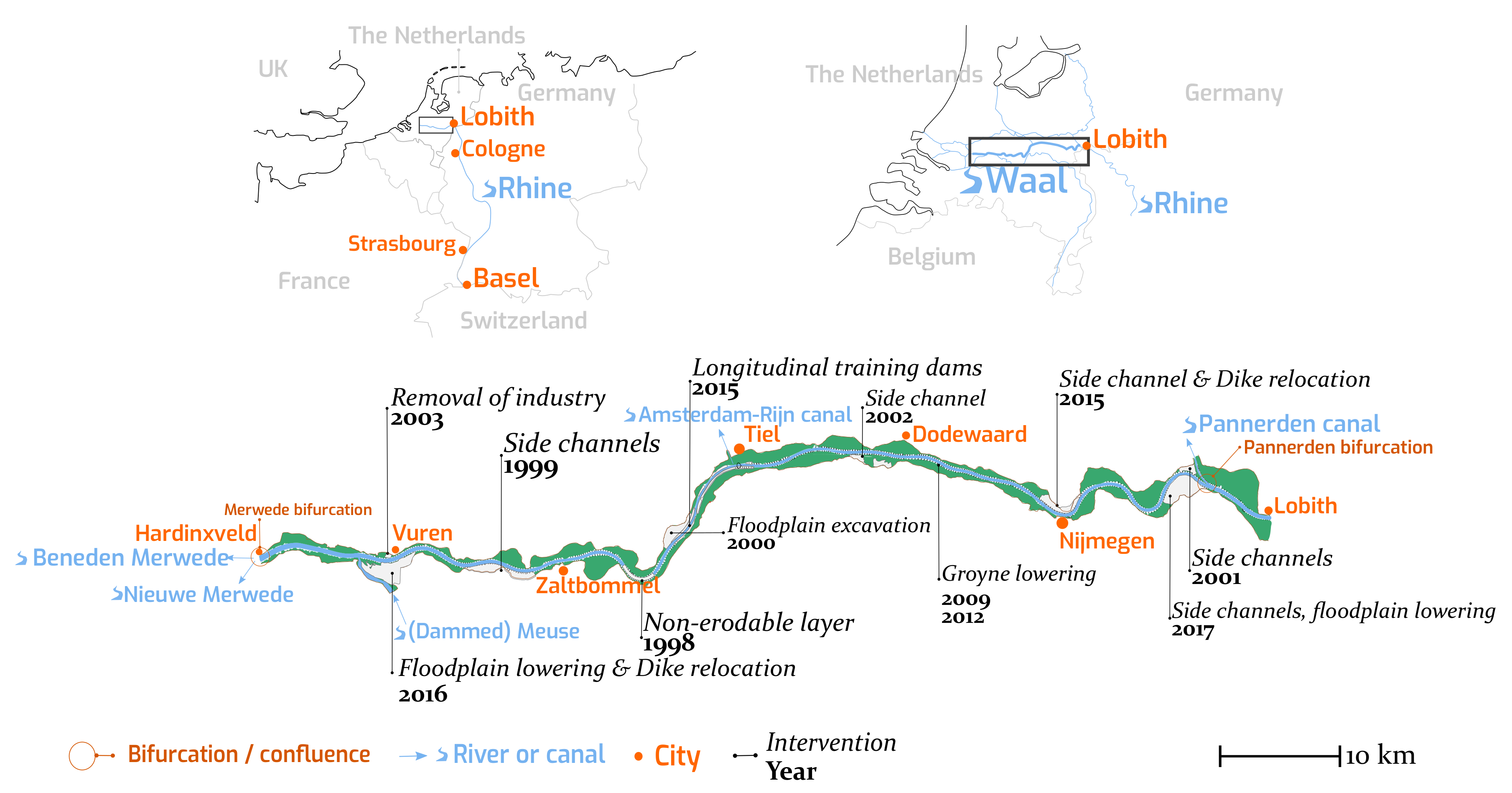
2.1. Case Study
2.2. Geographical Database
2.3. Hydraulic Data
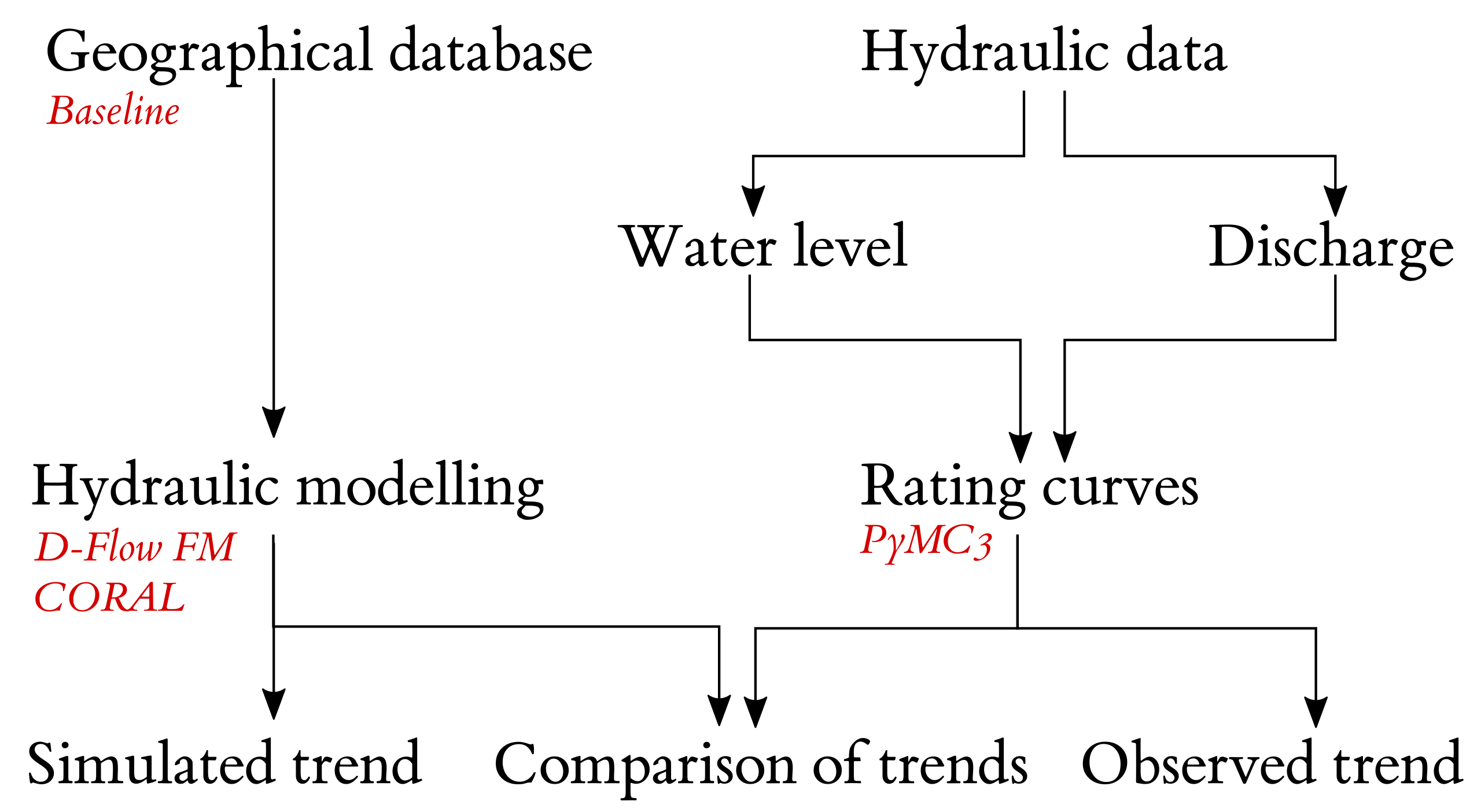
3. Methods
3.1. General Outline
3.2. Hydraulic Modelling
3.3. Rating Curve Construction
- For a, a moderately informative prior with a normal distribution was centred on the values obtained from deterministic optimisation.
- For b, a uniform distribution was chosen such that the values of b cannot overlap. This is necessary as the terms of (3) otherwise become interchangeable and therefore not identifiable by the algorithm.
- For p, an informative prior was centered on 1.7, following from rounding up from the expected value for p based on the Manning equation ().
- For , a non-informative half-Cauchy following [29].

| Parameter | Prior | Parameter | Prior | Parameter | Prior |
|---|---|---|---|---|---|
4. Results
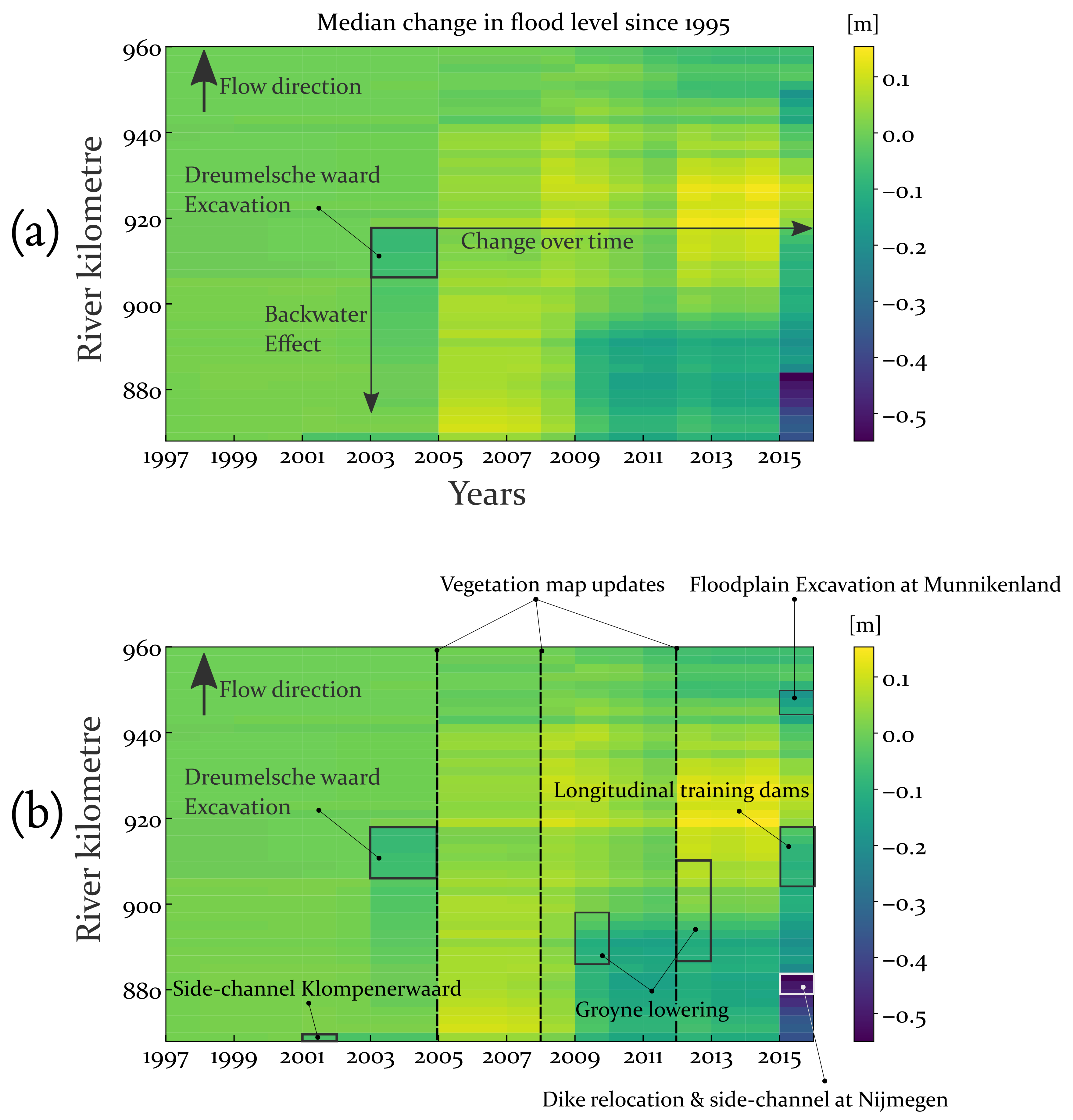
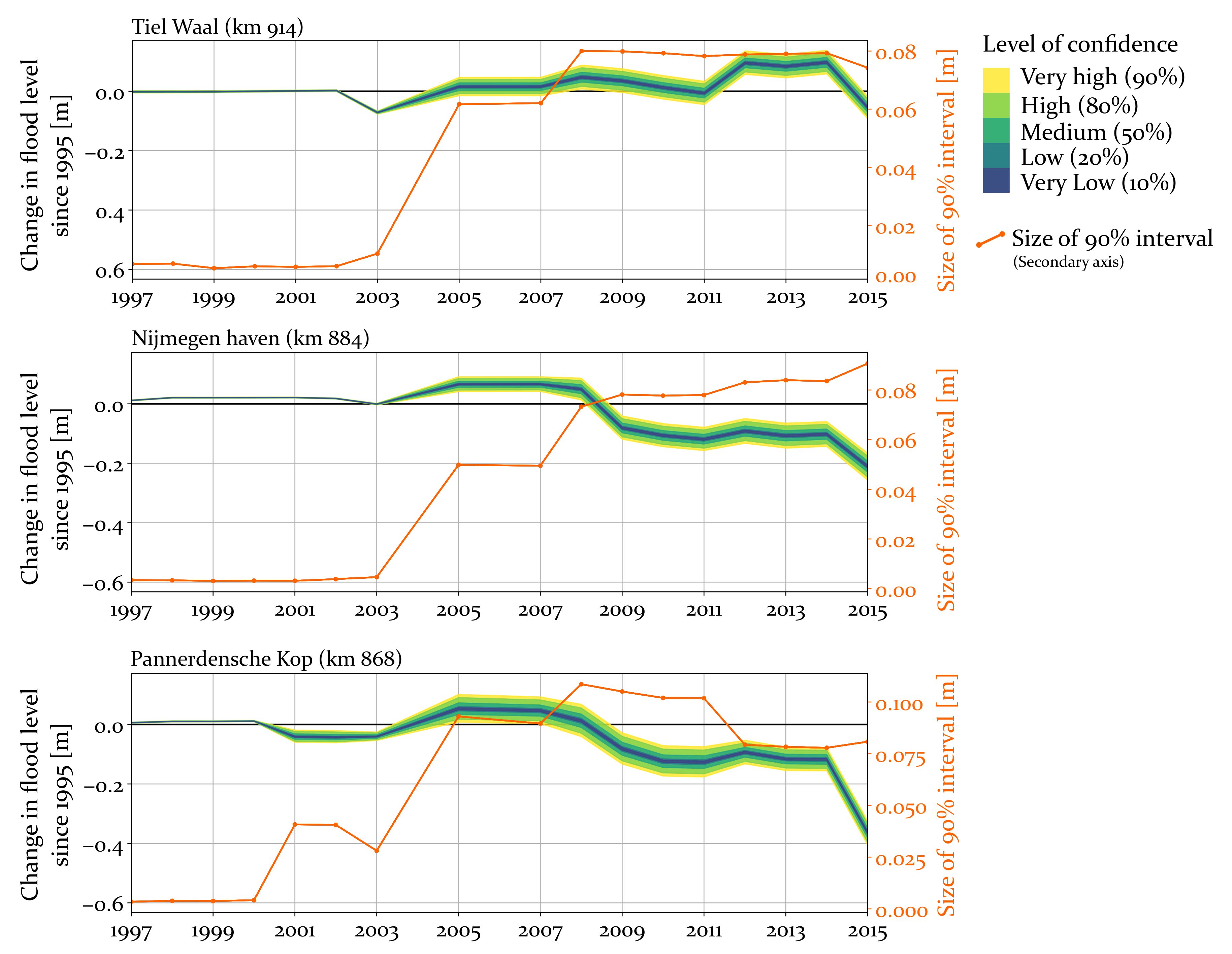
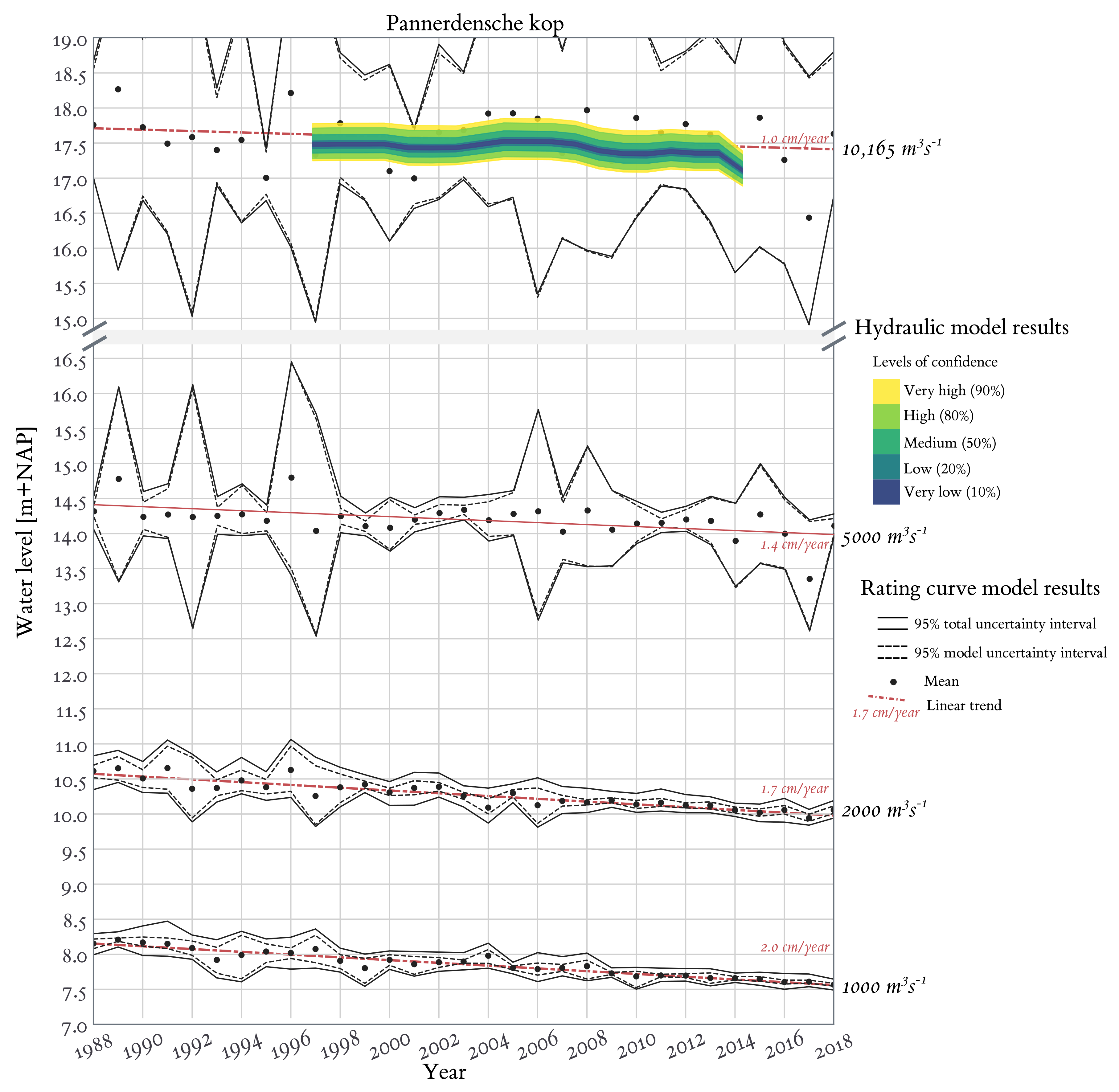
4.1. Simulated Trend
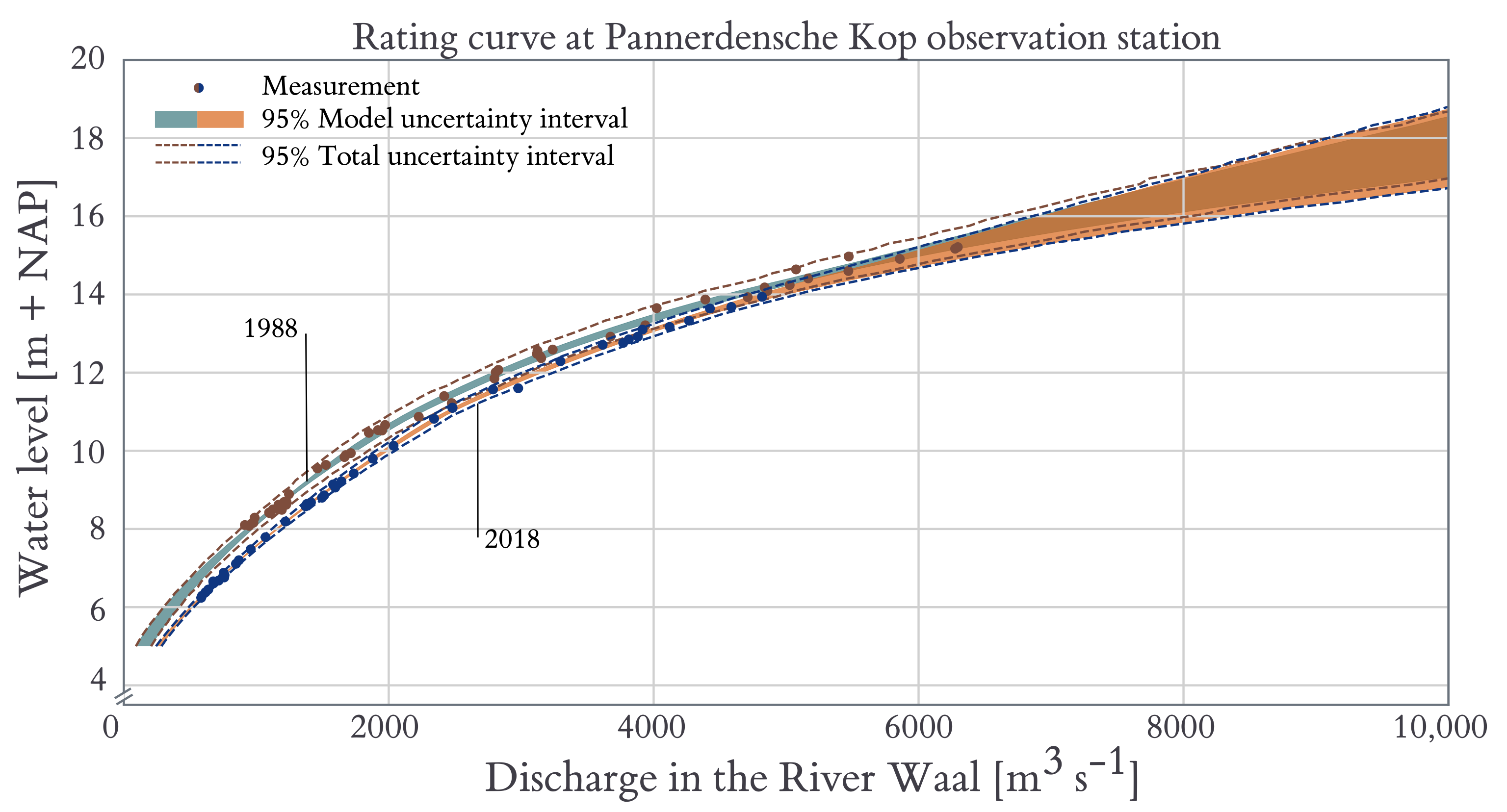
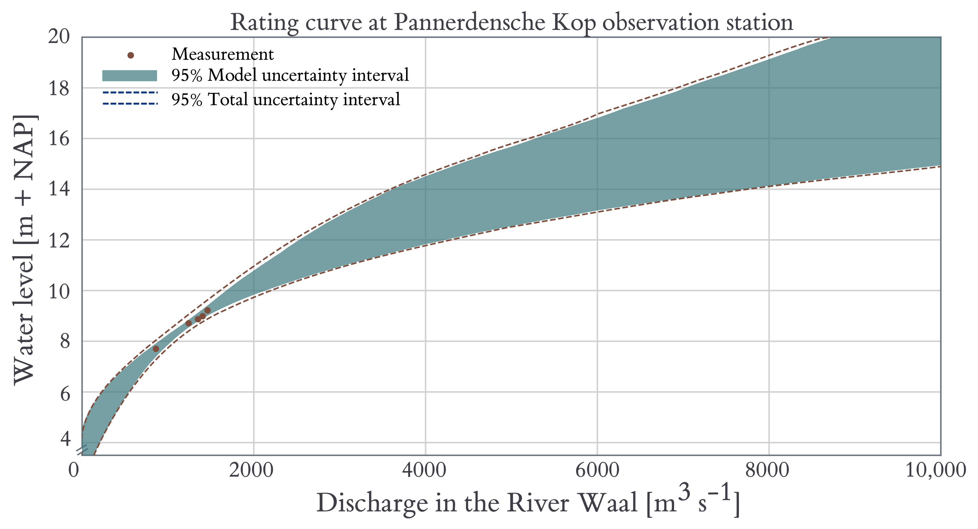
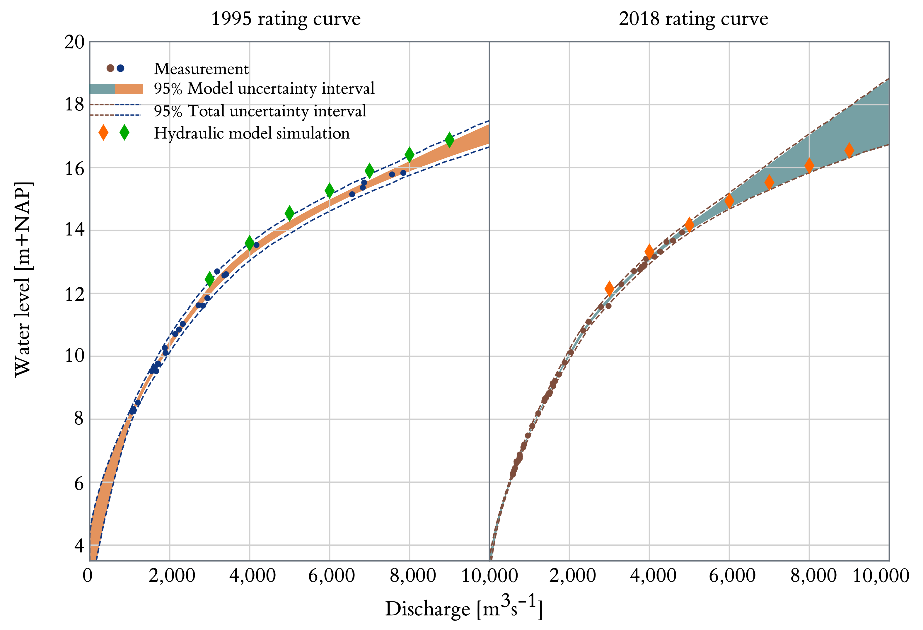
4.2. Rating Curves
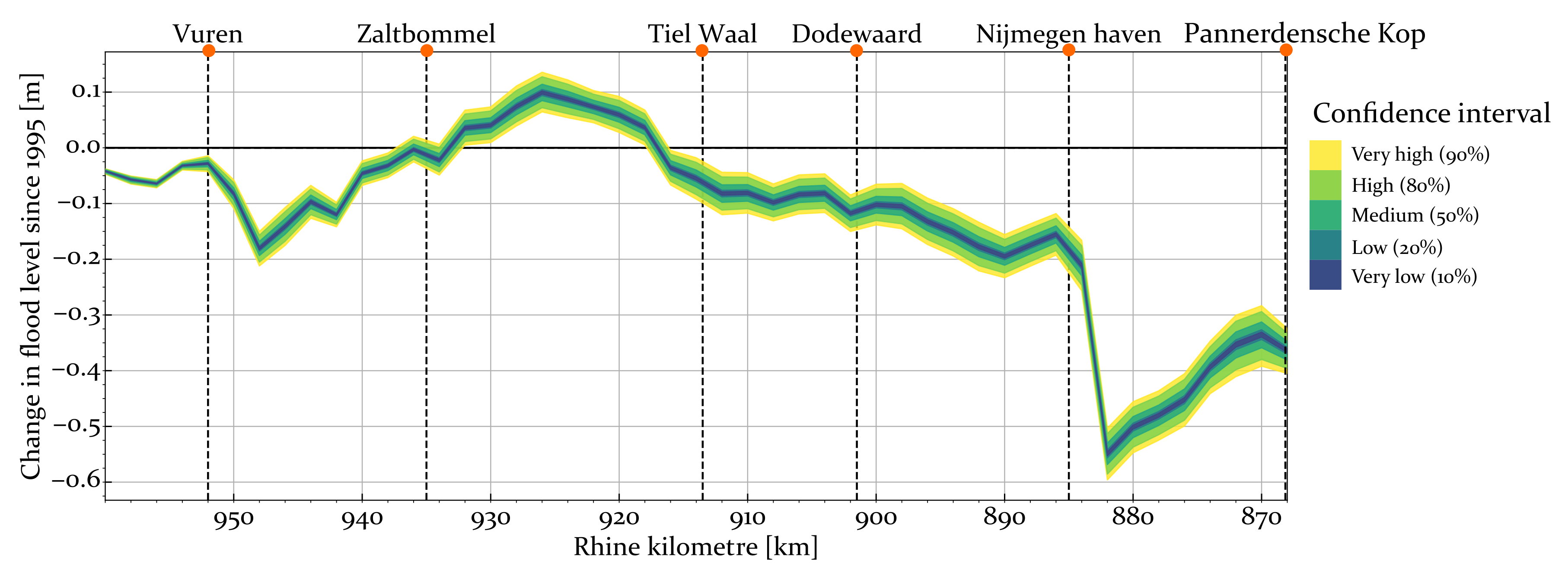
4.3. Long-Term Trends
5. Discussion
5.1. Explanations for the Discrepancy between Simulated and Observed Trends
5.2. Improvements to the Rating Curve Model
5.3. Reducing the Uncertainty of the Hydraulic Model
5.4. Interpreting the Implications of This Study
6. Conclusions
Author Contributions
Funding
Data Availability Statement
Acknowledgments
Conflicts of Interest
Appendix A. Table of Stochasts
| Class Code | Name | Parameters | |||
|---|---|---|---|---|---|
| Empirical distribution | |||||
| 612–637 | Alluvial bed | ||||
| Uniform distribution | |||||
| n/a | Classification map | ||||
| Triangular distributions | min | mean | max | ||
| 102 | Deep bed | 0.025 | 0.03 | 0.033 | |
| 104 | Natural side channel | 0.03 | 0.035 | 0.04 | |
| 105 | Side channel | 0.025 | 0.03 | 0.033 | |
| 106 | Pond/Harbor | 0.025 | 0.03 | 0.033 | |
| 111 | Sand bank | 0.025 | 0.03 | 0.033 | |
| 121 | Field | 0.02 | 0.03 | 0.04 | |
| Lognormal distributions | |||||
| 1201 | Production meadow | −3.18 | 0.47 | 2.40 | 0.77 |
| 1202 | Natural grass and hayland | −0.74 | 0.53 | −2.64 | 0.93 |
| 1203 | Herbaceous meadow | −1.64 | 0.32 | 2.59 | 0.33 |
| 1211 * | Thistle herb. Veg. | −1.29 | 0.33 | 1.05 | 0.43 |
| 1212 | Dry herbaceous vegetation | −0.59 | 0.39 | −3.06 | 0.65 |
| 1213 * | Brambles | −0.67 | 0.21 | −0.73 | 0.36 |
| 1214 * | Hairy willowherb | −1.89 | 0.56 | −0.25 | 0.49 |
| 1215 * | Reed herb. Veg. | 0.60 | 0.22 | −1.83 | 0.27 |
| 1221 | Wet herb. Veg. | −1.08 | 0.38 | −1.49 | 0.44 |
| 1222 * | Sedge | −1.32 | 0.67 | 0.04 | 0.63 |
| 1223 | Reed-grass | −0.92 | 0.86 | −2.19 | 0.16 |
| 1224 | Bulrush | −0.81 | 0.67 | 0.04 | 0.63 |
| 1225 * | Reed-mace | 0.37 | 0.23 | −1.12 | 0.57 |
| 1226 | Reed | 0.94 | 0.13 | −1.14 | 0.42 |
| 1231 | Softwood shrubs | 1.81 | 0.24 | −2.20 | 0.79 |
| 1232 | Willow plantation | 1.05 | 0.43 | −3.23 | 0.62 |
| 1233 | Thorny shrubs | 1.48 | 0.64 | −1.73 | 0.41 |
| 1241 * | Hardwood production forest | Deterministic | Deterministic | −4.68 | 0.67 |
| 1242 | Softwood production forest | Deterministic | Deterministic | −4.72 | 0.66 |
| 1243 * | Pine forest | Deterministic | Deterministic | −4.18 | 0.54 |
| 1244 | Hardwood forest | Deterministic | Deterministic | −3.45 | 0.77 |
| 1245 | Softwood forest | Deterministic | Deterministic | −3.04 | 0.99 |
| 1246 | Orchard low | 1.10 | 0.10 | −3.72 | 0.25 |
| 1247 | Orchard high | 1.78 | 0.21 | −4.61 | 0.12 |
| 1250 | Pioneer vegetation | −2.87 | 0.18 | −1.93 | 0.50 |
Appendix B. Table of Measurements
| Discharge [ms] | |||
|---|---|---|---|
| Year | n | Min. | Max. |
| 1988 | 50 | 914 | 6296 |
| 1989 | 53 | 708 | 2042 |
| 1990 | 41 | 741 | 4881 |
| 1991 | 29 | 628 | 4258 |
| 1992 | 8 | 889 | 1434 |
| 1993 | 20 | 1039 | 6958 |
| 1994 | 9 | 1231 | 4388 |
| 1995 | 26 | 1056 | 7844 |
| 1996 | 19 | 865 | 1835 |
| 1997 | 5 | 860 | 1461 |
| 1998 | 24 | 918 | 6077 |
| 1999 | 29 | 1184 | 5397 |
| 2000 | 38 | 1232 | 3736 |
| 2001 | 71 | 1150 | 6186 |
| 2002 | 55 | 1124 | 4652 |
| 2003 | 68 | 565 | 5863 |
| 2004 | 30 | 891 | 4623 |
| 2005 | 34 | 816 | 3740 |
| 2006 | 11 | 891 | 1596 |
| 2007 | 47 | 873 | 3690 |
| 2008 | 87 | 1042 | 2812 |
| 2009 | 62 | 688 | 2804 |
| 2010 | 66 | 1048 | 3894 |
| 2011 | 73 | 655 | 5451 |
| 2012 | 76 | 904 | 4440 |
| 2013 | 29 | 1245 | 3881 |
| 2014 | 40 | 932 | 2092 |
| 2015 | 31 | 755 | 3050 |
| 2016 | 38 | 768 | 3006 |
| 2017 | 44 | 735 | 2249 |
| 2018 | 44 | 584 | 4818 |
References
- Van Denderen, R.P.; Schielen, R.M.J.; Westerhof, S.G.; Quartel, S.; Hulscher, S.J.M.H. Explaining artificial side channel dynamics using data analysis and model calculations. Geomorphology 2019, 327, 93–110. [Google Scholar] [CrossRef] [Green Version]
- Collas, F.P.L.; Buijse, A.D.; Van den Heuvel, L.; Van Kessel, N.; Schoor, M.M.; Eerden, H.; Leuven, R.S.E.W. Longitudinal training dams mitigate effects of shipping on environmental conditions and fish density in the littoral zones of the river Rhine. Sci. Total Environ. 2018, 619–620, 1183–1193. [Google Scholar] [CrossRef] [PubMed]
- De Ruijsscher, T.; Naqshband, S.; Hoitink, T. Flow Bifurcation at a Longitudinal Training Dam: Effects on Local Morphology. E3S Web Conf. 2018, 40, 05020. [Google Scholar] [CrossRef]
- Berends, K.D.; Straatsma, M.W.; Warmink, J.J.; Hulscher, S.J.M.H. Uncertainty quantification of flood mitigation predictions and implications for interventions. Nat. Hazards Earth Syst. Sci. 2019, 19, 1737–1753. [Google Scholar] [CrossRef] [Green Version]
- Straatsma, M.W.; Kleinhans, M.G. Flood hazard reduction from automatically applied landscaping measures in RiverScape, a Python package coupled to a two-dimensional flow model. Environ. Model. Softw. 2018, 101, 102–116. [Google Scholar] [CrossRef]
- Klijn, F.; De Bruin, D.; De Hoog, M.C.; Jansen, S.; Sijmons, D.F. Design quality of room-for-the-river measures in the Netherlands: Role and assessment of the quality team (Q-team). Int. J. River Basin Manag. 2013, 11, 287–299. [Google Scholar] [CrossRef]
- Thirel, G.; Andréassian, V.; Perrin, C. On the need to test hydrological models under changing conditions. Hydrol. Sci. J. 2015, 60, 1165–1173. [Google Scholar] [CrossRef]
- Beven, K. Facets of uncertainty: Epistemic uncertainty, non-stationarity, likelihood, hypothesis testing, and communication. Hydrol. Sci. J. 2016, 61, 1652–1665. [Google Scholar] [CrossRef] [Green Version]
- Blöschl, G.; Bierkens, M.F.P.; Chambel, A.; Cudennec, C.; Destouni, G.; Fiori, A.; Kirchner, J.W.; McDonnell, J.J.; Savenije, H.H.G.; Sivapalan, M.; et al. Twenty-three unsolved problems in hydrology (UPH)—A community perspective. Hydrol. Sci. J. 2019, 64, 1141–1158. [Google Scholar] [CrossRef] [Green Version]
- Oreskes, N.; Belitz, K. Philosphical issues in Model Assessment. In Model Validation: Perspectives in Hydrological Science; Anderson, M.G., Bates, P.D., Eds.; John Wiley and Sons Ltd.: New York, NY, USA, 2001; pp. 23–41. [Google Scholar]
- Van der Sluijs, J.P. A way out of the credibility crisis of models used in integrated environmental assessment. Futures 2002, 34, 133–146. [Google Scholar] [CrossRef] [Green Version]
- Jakeman, A.J.; Letcher, R.A.; Norton, J.P. Ten iterative steps in development and evaluation of environmental models. Environ. Model. Softw. 2006, 21, 602–614. [Google Scholar] [CrossRef] [Green Version]
- Uusitalo, L.; Lehikoinen, A.; Helle, I.; Myrberg, K. An overview of methods to evaluate uncertainty of deterministic models in decision support. Environ. Model. Softw. 2015, 63, 24–31. [Google Scholar] [CrossRef] [Green Version]
- Maier, H.R.; Guillaume, J.H.A.; Van Delden, H.; Riddell, G.A.; Haasnoot, M.; Kwakkel, J.H. An uncertain future, deep uncertainty, scenarios, robustness and adaptation: How do they fit together? Environ. Model. Softw. 2016, 81, 154–164. [Google Scholar] [CrossRef]
- Straatsma, M.W.; Van der Perk, M.; Schipper, A.M.; De Nooij, R.J.W.; Leuven, R.S.E.W.; Huthoff, F.; Middelkoop, H. Uncertainty in hydromorphological and ecological modelling of lowland river floodplains resulting from land cover classification errors. Environ. Model. Softw. 2013, 42, 17–29. [Google Scholar] [CrossRef]
- Warmink, J.J.; Booij, M.J.; Van der Klis, H.; Hulscher, S.J.M.H. Quantification of uncertainty in Design water levels due to uncertain bed form roughness in the Dutch rivier Waal. Hydrol. Process. 2013, 27, 1646–1663. [Google Scholar] [CrossRef]
- Becker, A.; Scholten, M.; Kerkhoven, D.; Spruyt, A. Das Behördliche Modellinstrumentarium der Niederlande. In 37. Dresdner Wasserbaukolloquium 2014 “Simulationsverfahren und Modelle für Wasserbau und Wasserwirtschaft”; Stamm, J., Ed.; Dresden, Germany, 2014; pp. 539–548. [Google Scholar]
- Kroekenstoel, D. Rivierkundig Beoordelingskader voor Ingrepen in de Grote Rivieren; v2.01; Technical Report; Rijkswaterstaat: Lelystad, The Netherlands, 2009; v2.01; Technical Report. [Google Scholar]
- Buschman, F.; Blom, A.; Van Dijk, T.; Kleinhans, M.; Van der Mark, R. Informatiebehoefte en Aanbevelingen voor Monitoring in de Bovendeltade Rijn; Technical Report; Deltares: Delft, The Netherlands, 2017. [Google Scholar]
- Warmink, J.J.; Straatsma, M.W.; Huhoff, F.; Booij, M.J.; Hulscher, S.J.M.H. Uncertainty of design water levels due to combined bed form and vegetation roughness in the Dutch River Waal. J. Flood Risk Manag. 2013, 6, 302–318. [Google Scholar] [CrossRef]
- Kernkamp, H.W.J.; Van Dam, A.; Stelling, G.S.; De Goede, E.D. Efficient scheme for the shallow water equations on unstructured grids with application to the Continental Shelf. Ocean. Dyn. 2011, 61, 1175–1188. [Google Scholar] [CrossRef]
- Warmink, J.J.; van der Klis, H.; Booij, M.J.; Hulscher, S.J.M.H. Identification and quantification of uncertainties in a hydrodynamic river model using expert opinion elicitation. Water Resour. Manag. 2011, 25, 601–622. [Google Scholar] [CrossRef] [Green Version]
- Berends, K.D.; Warmink, J.J.; Hulscher, S.J.M.H. Efficient uncertainty quantification for impact analysis of human interventions in rivers. Environ. Model. Softw. 2018, 107, 50–58. [Google Scholar] [CrossRef] [Green Version]
- Berends, K. CORAL: kdberends/coral: v0.1-PhD. 2020. Available online: https://0-doi-org.brum.beds.ac.uk/10.5281/ZENODO.3749855 (accessed on 13 July 2021).
- Mansanarez, V.; Renard, B.; Le Coz, J.; Lang, M.; Darienzo, M. Shift Happens! Adjusting Stage-Discharge Rating Curves to Morphological Changes at Known Times. Water Resour. Res. 2019, 55, 2876–2899. [Google Scholar] [CrossRef]
- Reitan, T.; Petersen-Øverleir, A. Dynamic rating curve assessment in unstable rivers using Ornstein-Uhlenbeck processes. Water Resour. Res. 2011, 47. [Google Scholar] [CrossRef]
- Le Coz, J.; Renard, B.; Bonnifait, L.; Branger, F.; Boursicaud, R.L. Combining hydraulic knowledge and uncertain gaugings in the estimation of hydrometric rating curves: A Bayesian approach. J. Hydrol. 2014, 509, 573–587. [Google Scholar] [CrossRef] [Green Version]
- Hoffman, M.D.; Gelman, A. The No-U-Turn Sampler: Adaptively Setting Path Lengths in Hamiltonian Monte Carlo. J. Mach. Learn. Res. 2014, 15, 1593–1623. [Google Scholar]
- Gelman, A. Prior distributions for variance parameters in hierarchical models. Bayesian Anal. 2006, 1, 515–533. [Google Scholar] [CrossRef]
- Ten Brinke, W.B.M.; Gölz, E. Bed Level Changes and Sediment Budget of the Rhine Near the German-Dutch Border; Technical Report; German Federal Institute of Hydrology (BFG), Institute for Inland Water Management and Waste Water Treatment = Ministerie van Verkeer en Waterstaat, Rijkswaterstaat, Rijksinstituut voor Integraal Zoetwaterbeheer en Afvalwaterbehandeling (RWS, RIZA): Lelystad, The Netherlands, 2001. [Google Scholar]
- Chbab, E.H. How extreme were the 1995 flood waves on the rivers Rhine and Meuse? Phys. Chem. Earth 1995, 20, 455–458. [Google Scholar] [CrossRef]
- Di Baldassarre, G.; Montanari, A. Uncertainty in river discharge observations: A quantitative analysis. Hydrol. Earth Syst. Sci. 2009, 13, 913–921. [Google Scholar] [CrossRef] [Green Version]
- Domeneghetti, A.; Castellarin, A.; Brath, A. Assessing rating-curve uncertainty and its effects on hydraulic model calibration. Hydrol. Earth Syst. Sci. Discuss. 2011, 8, 10501–10533. [Google Scholar] [CrossRef]
- Petersen-Øverleir, A. Modelling stage—Discharge relationships affected by hysteresis using the Jones formula and nonlinear regression. Hydrol. Sci. J. 2006, 51, 365–388. [Google Scholar] [CrossRef] [Green Version]
- McMillan, H.; Freer, J.; Pappenberger, F.; Krueger, T.; Clark, M. Impacts of uncertain river flow data on rainfall-runoff model calibration and discharge predictions. Hydrol. Process. 2010. [Google Scholar] [CrossRef]
- Romanowicz, R.; Beven, K.J.; Tawn, J. Bayesian Calibration of Flood Inundation Models. In Floodplain Processes; Anderson, M.G., Walling, D.E., Bates, P.D., Eds.; John Wiley and Sons Ltd.: London, UK, 1996; pp. 333–360. [Google Scholar]
- Pappenberger, F.; Beven, K.J. Ignorance is bliss: Or seven reasons not to use uncertainty analysis. Water Resour. Res. 2006, 42. [Google Scholar] [CrossRef]
- Werner, M.G.F.; Hunter, N.M.; Bates, P.D. Identifiability of distributed floodplain roughness values in flood extent estimation. J. Hydrol. 2005, 314, 139–157. [Google Scholar] [CrossRef]
- Klemes, V. Operational testing of hydrological simulation models. Hydrol. Sci. J. 1986, 31, 13–24. [Google Scholar] [CrossRef]
- Thirel, G.; Andréassian, V.; Perrin, C.; Audouy, J.N.; Berthet, L.; Edwards, P.; Folton, N.; Furusho, C.; Kuentz, A.; Lerat, J.; et al. Hydrology under change: An evaluation protocol to investigate how hydrological models deal with changing catchments. Hydrol. Sci. J. 2015, 60, 1184–1199. [Google Scholar] [CrossRef]
- Saltelli, A.; Bammer, G.; Bruno, I.; Charters, E.; Di Fiore, M.; Didier, E.; Espeland, W.N.; Kay, J.; Lo Piano, S.; Mayo, D.R.P., Jr.; et al. Five ways to ensure that models serve society: A manifesto. Nature 2020, 582, 482–484. [Google Scholar] [CrossRef]
- Salvatier, J.; Wiecki, T.V.; Fonnesbeck, C. Probabilistic programming in Python using PyMC3. PeerJ Comput. Sci. 2016, 2, e55. [Google Scholar] [CrossRef] [Green Version]


Publisher’s Note: MDPI stays neutral with regard to jurisdictional claims in published maps and institutional affiliations. |
© 2021 by the authors. Licensee MDPI, Basel, Switzerland. This article is an open access article distributed under the terms and conditions of the Creative Commons Attribution (CC BY) license (https://creativecommons.org/licenses/by/4.0/).
Share and Cite
Berends, K.D.; Gensen, M.R.A.; Warmink, J.J.; Hulscher, S.J.M.H. Multidecadal Analysis of an Engineered River System Reveals Challenges for Model-Based Design of Human Interventions. CivilEng 2021, 2, 580-598. https://0-doi-org.brum.beds.ac.uk/10.3390/civileng2030032
Berends KD, Gensen MRA, Warmink JJ, Hulscher SJMH. Multidecadal Analysis of an Engineered River System Reveals Challenges for Model-Based Design of Human Interventions. CivilEng. 2021; 2(3):580-598. https://0-doi-org.brum.beds.ac.uk/10.3390/civileng2030032
Chicago/Turabian StyleBerends, Koen D., Matthijs R. A. Gensen, Jord J. Warmink, and Suzanne J. M. H. Hulscher. 2021. "Multidecadal Analysis of an Engineered River System Reveals Challenges for Model-Based Design of Human Interventions" CivilEng 2, no. 3: 580-598. https://0-doi-org.brum.beds.ac.uk/10.3390/civileng2030032