Article

A Neural Network Inverse Optimization Procedure for Constitutive Parameter Identification and Failure Mode Estimation of Laterally Loaded Unreinforced Masonry Walls

by
Qudama Albu-Jasim
1,* and
George Papazafeiropoulos
2
1
Department of Civil and Environmental Engineering, College of Engineering, Texas A&M University, 400 Bizzell Street, College Station, TA 77840, USA
2
Department of Structural Engineering, Zografou Campus, National Technical University of Athens, 9, Iroon Polytechniou Street, 15780 Athens, Greece
*
Author to whom correspondence should be addressed.
Submission received: 12 September 2021 / Revised: 19 October 2021 / Accepted: 20 October 2021 / Published: 3 November 2021
(This article belongs to the Special Issue Early Career Stars in Civil Engineering)

Abstract

:
A new Neural Network Optimization (NNO) algorithm for constitutive material parameter identification based on inverse analysis of experimental tests of small-scale masonry prisms under compressive loads is presented. The Concrete Damaged Plasticity (CDP) constitutive model is used for the brick and mortar of the Unreinforced Masonry (URM) walls. By comparisons with experimental data taken from laboratory tests, it is demonstrated that the constitutive parameters calibrated by application of the proposed inverse optimization procedure on the small-scale (prism) experimental results are sufficiently accurate to allow for the prediction of the mechanical response of large-scale URM walls subject to compressive and lateral loads. This eliminates the need for large-scale URM wall experimental tests for the identification of their material properties, making the calibration process more economic. After verifying the accuracy of the calibrated constitutive parameters based on the above comparisons, a numerical parametric study is performed for the investigation of the effect of material behavior and geometrical aspect ratios on the failure mechanisms of large-scale URM walls.

1. Introduction

Extensive laboratory tests have been carried out in the past decades to evaluate the behavior of masonry structures [1,2,3]. Various constitutive models for masonry walls and their constituents have been used in the past. For example, Chaimoon and Attard [4] introduced a numerical formulation to analyze URM walls under shear compression fracture. The inelastic failure surface was modeled using a Mohr Coulomb failure surface with a tension cutoff and a linear compression cap. The results were verified by comparison with experimental response of shear walls under shear compression loading. However, due to the nature of the material of bricks and mortar comprising URM walls, which is similar to that of concrete, the majority of the constitutive models that are used for analyzing the bricks and mortar are identical to, or variations of, those of concrete. In [5] the capability of smeared crack models in capturing the strength and various failure mechanisms of reinforced masonry shear walls is assessed. The model showed excellent performance with respect to flexure dominated behavior, but it had a major drawback in capturing the brittle shear behavior. A combination of plasticity and damage applied to modeling of concrete failure has been used in [6]. Various contributions [7,8,9,10] led to the development of the Concrete Damaged Plasticity (CDP) model, which includes scalar (isotropic) damage and stiffness recovery effects under cyclic loading. This constitutive model is ideal for cases in which lateral loads such as earthquakes are present, since it accounts for the degradation of the elastic stiffness of concrete induced by its plastic straining both in tension and compression. Damage mechanics based constitutive models have also been used for modeling of the in-plane loaded brick masonry shear walls, where both mortar damage and decohesion between brick and mortar are considered in an effort to simulate the opening and frictional sliding [11].
To minimize the error between the observation-based datasets and model parameters, inverse methods have been applied to identify and characterize the material properties in the constitutive models. For example, Chisari et al. [12] tested a detailed nonlinear brick masonry mesoscale model subjected to diagonal compression loads and compared its results with those of a finite element (FE) model to identify the material parameters by minimizing the errors between the experiment and numerical data. In addition, they have developed techniques for model and material parameter identification of masonry structures [13,14] and have successfully performed parameter identification considering uncertainties in the experimental data and response sensitivities to model parameters, from the shear strength estimation of a masonry panel subjected to a diagonal compression test [15]. Given the nature of the failure of quasi brittle materials, such as bricks and mortar in URM walls, which is characterized by the growth and coalescence of microcracks, eventually leading to the formation of narrow damage zones, indirect inverse identification methods have also been used. Carmeliet [16] determined the damage material parameters by minimizing the errors between the design variable of laboratory tests and prior information from the gradient damage model parameters estimated by Markov estimator method, and a reasonable agreement between the experimental and numerical results is achieved. Despite the fact that FE modeling is the most common means of numerical simulation of URM walls, other numerical methodologies can be found in the literature as well; e.g., Caliò et al. [17] used a discrete-element model based on the concept of macro-element discretization to simulate masonry buildings behavior and investigate nonlinear behavior response subjected to in-plane earthquake loads.
Besides the above, a variety of optimization algorithms have been used and tested for inverse analysis for estimation of material parameters based on experimental results. For example, Muñoz-Rojas et al. [18] identified the material parameters of Gurson’s damage model by fitting the numerical to the experimental force vs. displacement curves from tensile tests using a specially configured genetic optimization algorithm, designed to avoid local minima through automatic adjustment of the elitism and mutation rates depending on the population diversity. Nazari and Sanjayan [19] presented an approach for material parameter estimation using different optimization algorithms to predict compressive strength of geopolymer mortar, paste and concrete. Toropov and Garrity [20] proposed an optimization method to identify material parameters that are based on the response of relatively “nontrivial” large scale masonry elements. Sarhosis and Sheng [21] used an optimization procedure to estimate the parameters of masonry constitutive models by minimizing the difference between experimental results from the load testing of large clay brick low bond strength masonry wall panels and data from their numerical simulation. The estimated parameters were used to validate the numerical model against another experimental wall panel test, and good correlation between the experimental and numerical results was found.
Apart from the constitutive behavior of the brick and mortar materials, the effect of various parameters on the failure mechanisms of URM walls has also been investigated. For example, the influence of the wall aspect ratio on the failure mechanism of URM walls under lateral loads has been largely investigated in some early studies structures [22,23]. Apart from these, Magenes and Calvi [24] examined the strength, deformability, and energy dissipation capacity of URM walls and proposed simplified methodologies for their evaluation, based on experimental and numerical data. Agnihotri et al. [25] studied the stability and safety of URM walls after being damaged by combined cyclic in-plane and monotonic out-of-plane loading, considering different slenderness ratios and aspect ratios, through nonlinear finite element models. The CDP model in ABAQUS 2021HF5 (6.21-6) was used to simulate the inelastic behavior of masonry. Salmanpour et al. [26] carried out experimental static cyclic shear tests on full scale URM walls to investigate the effects of various factors, i.e., unit type, vertical pre compression level, aspect ratio, size, and boundary conditions, on the displacement capacity of URM walls. Howlader et al. [27] investigated the shear behavior of URM walls with a semicircular arch opening subjected to the in-plane loads numerically. Aspects of the complex nature of the URM walls including their potential for shear cracking and/or sliding and rocking and/or toe crushing were taken into account.
From the aforementioned paragraphs, it is obvious that, since URM walls are structural elements which generally show brittle and nonlinear inelastic mechanical response, formulating constitutive models and calibrating material parameters in the constitutive models is essential to provide reliable predictions of the response of URM walls under mechanical loads. The CDP constitutive model [7,8,9] that describes only the plasticity stage is used in this study to analyze the mechanical response of masonry structures. The four most influential parameters of the CDP material model (i.e., the dilatancy angle ψ, the flow potential eccentricity of the brick and the mortar ε, the ratio of initial equibiaxial compressive yield stress to initial uniaxial compressive yield stress σb0c0, the ratio of the second stress invariant on the tensile meridian to that on the compressive meridian at initial yield of the brick and the mortar Kc) are used for the prism calibration analysis. The selection of these CDP parameters as well as their typical ranges have been discussed in several studies in the literature based on calibrations from experimental data [28,29,30,31]. The agreement between the experimental and numerical results is enforced through a novel Neural Network Optimization algorithm (NNO). In this study, the objective function is applied using the least squares technique, which minimizes the sum of the squares of the differences between experiment based measurements and the calculated response of the model [32,33]. A table containing the references of the literature review, along with corresponding keywords and findings is presented in Appendix A of the present study.
Despite the variety of the aforementioned studies, in which efforts are made towards understanding the response of URM walls, only few studies have addressed the possibility of predicting the response of an entire wall system (macroscale) based on the experimental data taken from experimental tests of a masonry prism (mesoscale) model. This possibility will lead to large financial gains, through reducing and even cutting the costs associated with complex experimental testing, as experimentation with macroscale specimens is totally avoided and replaced by studies using only mesoscale experimental setup. The present study tries to address the above research gap. This study is comprised of two parts. Firstly, the material properties of the CDP model are calibrated from an experimental stress strain curve obtained from a uniaxial compression test of a small scale prism. The material properties that correspond to the optimum fit between the numerical and experimental curves are found using the proposed NNO algorithm. The calibrated material properties are subsequently used for a parametric study of the response of URM walls under lateral loads. The calibrated material parameters and model is first validated from two experimental tests on the shear response of URM walls. A good agreement between numerical and experimental results demonstrates the accuracy of the material properties that are used in the FE models, and therefore the accuracy of the proposed NNO algorithm. A parametric study is finally performed to identify the factors that have a major effect on the shear response of URM walls and also estimate the failure modes of the URM walls. One of the advantages of this study are that it eliminates the need for large scale experiments for estimating the material parameters through inverse optimization, which is a relatively expensive experimental practice. On the contrary, in this study only small scale (prism) experiments are used for this purpose. It is proved that the optimum material parameters based on these small scale experiments can then be used to make predictions in large scale experiments. The proposed research has shown a great impact in the assessment of mechanical properties of a masonry prism (mesoscale) that allow to (i) verify the capacity of the model to predict the response of the entire wall system (macroscale) (ii) open the possibility of reducing and even cutting the costs associated with complex experimental testing.

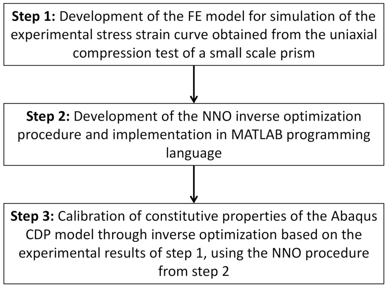
2. Materials and Methods

2.1. General

The constitutive properties of the CDP model, which is available in ABAQUS 2021HF5 (6.21-6) FE code, are calibrated so that the numerical stress strain curve (SSnum) fits the corresponding experimental curve (SSexp). This is done through the implementation of an inverse optimization analysis, whereby an optimization procedure is implemented that minimizes the least square error between the numerical and experimental data. ABAQUS 2021HF5 (6.21-6) FEA software [34] is used for performing the structural analyses, and MATLAB R2021a [35] is used for the implementation of the NNO optimization procedure, which is used for carrying out the optimization process. MATLAB R2021a is appropriately coupled with ABAQUS 2021HF5 (6.21-6) by using Abaqus2Matlab v.2.0 [36], a novel software that can transfer model data and results between ABAQUS 2021HF5 (6.21-6) with MATLAB R2021a and vice versa, leading thus to a user-friendly integrated simulation and programming environment. A flowchart of the various steps that are presented in this section is shown in Figure 1.

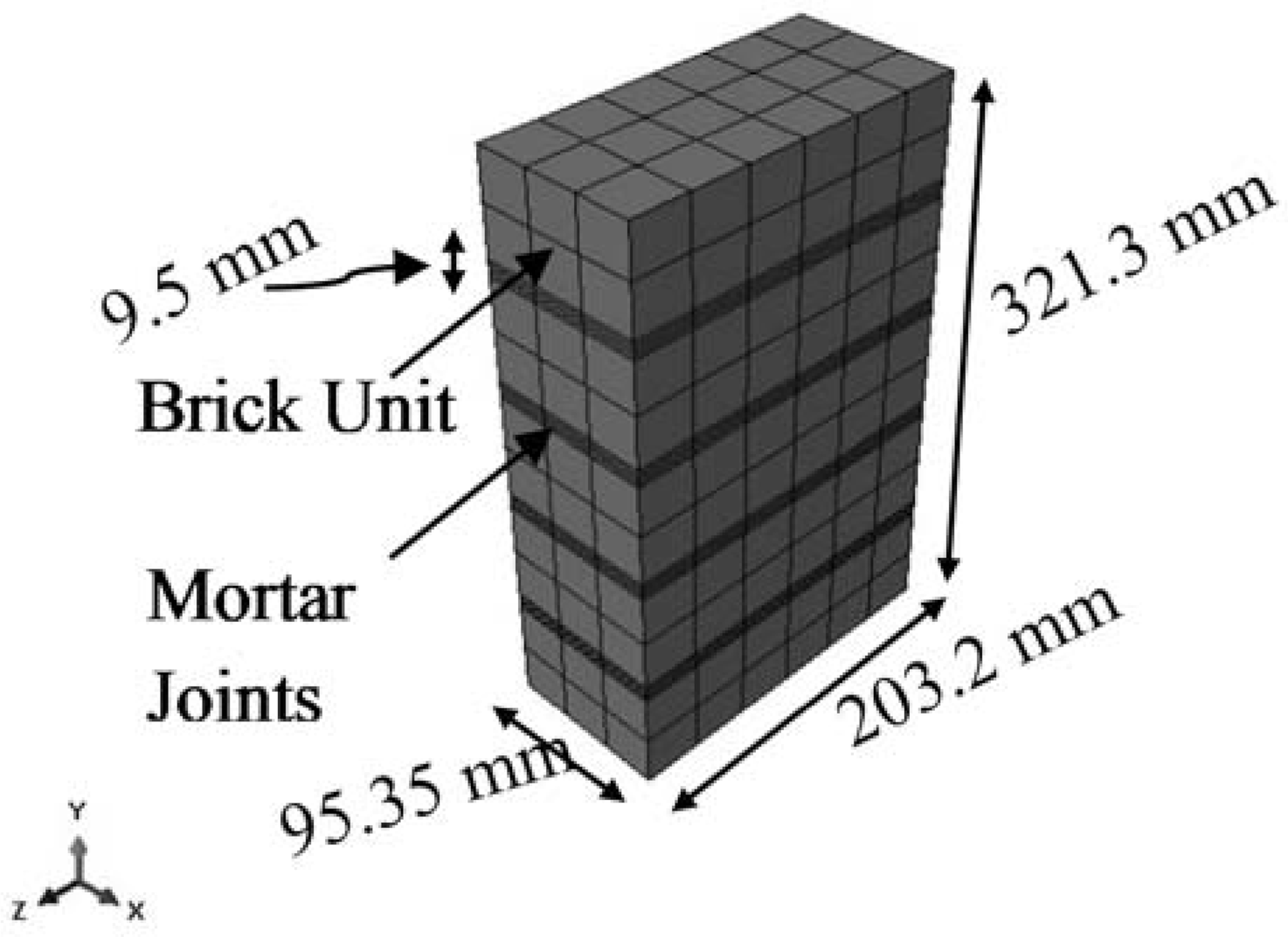
2.2. Description of the Prism Model

The model is comprised of 5 bricks and 4 layers of mortar between the former. The cross section dimensions of the prism are 9.525 cm × 20.32 cm × 32.13 cm and the mortar thickness between the bricks is 0.95 cm [1]. The prism is fixed at its bottom and at the top a uniform displacement is imposed. Since the compressive strength is lower parallel to the bed joints compared to that in the normal direction, the interfaces between the bricks and mortar in the prism model are assumed to be fully bonded [3]. The ABAQUS 2021HF5 (6.21-6) model of the prism is discretized in 530 3D solid elements (C3D8R), defined by 1073 nodes (see Figure 2). An appropriate mesh sensitivity analysis has been performed to ensure that the mesh refinement does not affect significantly the final results. The constitutive behavior of both the bricks and the mortar is defined by the ABAQUS 2021HF5 (6.21-6) CDP model, the parameters of which are treated as design variables of the NNO problem. The Poisson ratio of the bricks is considered to be equal to 0.2 whereas the Poisson ratio of the mortar is treated as a design variable ranging from 0.1 to 0.4. The viscosity parameter μ which is used for the visco-plastic regularization of the concrete constitutive equations in ABAQUS/Standard (v. 2021HF5, 6.21-6) is considered to be zero. It is assumed that the other parameters of the CDP model that define the flow potential and yield surface are considered to be identical for the brick and mortar materials, since more than one type of loading (i.e., other than compression test that is considered in the present study) have to be applied on the prism specimens, in order to be able to identify the different effect of the brick and mortar material on the total response of the prism specimen, enabling the possibility of calibrating the constitutive properties of each one of these two materials. Furthermore, the bricks and the mortar layers are considered to be tied across their interfaces. The stress-strain curve in compression for both brick and mortar material is defined only by specifying the initial yield stress value at an inelastic (crushing) strain equal to 0.0. This corresponds to a simple elastoplastic behavior in the compression post cracking regime. Tension stiffening for both brick and mortar materials is modeled as a linearly decreasing post failure stress/cracking-strain relationship, defined by the direct failure stress σt0 at zero direct cracking strain, and by the remaining direct stress 0.1σt0 at direct cracking strain equal to εtf. εtf is the strain at which the material is considered to have failed in tension. Moreover, damage factors in compression and tension have not been considered, since they control only the unloading and reloading response of the brick and/or mortar materials, i.e., cyclic response. As the compressive loading applied to the prism specimen in this study is only monotonic, the aforementioned parameters can be ignored. Static analysis is performed to obtain the response of the prism due to the imposed displacement. More specifically, there are 10 design variables in this optimization problem:
  • The moduli of elasticity (EC, EM) of the brick and the mortar respectively;
  • The dilation angle in the p–q plane of the brick and the mortar ψ;
  • The flow potential eccentricity of the brick and the mortar ε;
  • The ratio of initial equibiaxial compressive yield stress to initial uniaxial compressive yield stress σb0c0;
  • The ratio of the second stress invariant on the tensile meridian to that on the compressive meridian at initial yield of the brick and the mortar Kc;
  • The Poisson ratio of the mortar, νM, since it has a major influence on the behaviour of masonry;
  • The initial yield stress value of brick material in compression, σc0,C for crushing strain equal to 0.0.
  • The initial yield stress value of mortar material in compression, σc0,M for crushing strain equal to 0.0.
  • The cracking strain in tension, εtf, for failure stress value equal to 0.1σt0, where σt0 is the failure stress value for cracking strain equal to 0.0. σt0 is assumed to be equal to 0.1σc0,C for brick material and 0.1σc0,M for mortar material.
The upper and lower limits are set for the design variables based on the literature and are shown in Table 1.

2.3. Proposed Methodology for Material Parameter Identification

The NNO algorithm that has been used for the inverse optimization process employs a novel technique that combines common inverse optimization analysis and neural network training. The essential steps are illustrated in the algorithm outline presented in Algorithm 1.
Algorithm 1. Neural Optimization.
1: Read the experimental stress-strain curve SSexp
2: Define M combinations of the 10 design variables
3: for k from 1 to M
4:   Perform simulation in ABAQUS corresponding to parameters xk
5:   Read kth stress-strain curve and append it in array SSraw
6: end for
7: Initialize err = +∞ and j = 1
8: while j ≤ maxIter & err > tol
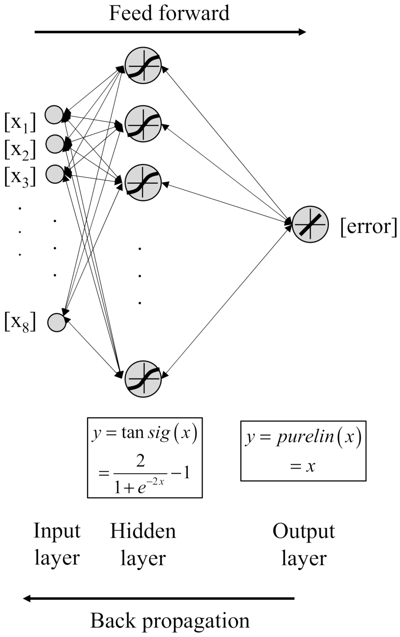
9:   Train an Artificial Neural Network (ANN), net, as follows:
     ● Training function: Bayesian regularization
     ● Input training data: xk, k = 1…M
     ● Output training data: norm(SSexp − SSraw,k ), k = 1…M
10:   Find optimum values xj by Interior Point optimization as follows:
     ● Objective function: the ANN net, fANN (see previous step)
     ● Initial guess: xj−1
     ● Constraints: xi,lb ≤ xi,j ≤ xi,ub
11:   Perform simulation in ABAQUS corresponding to parameters xj
12:   Read stress-strain curve and append it in array SSraw
13:   Update err = norm(SSexp − SSraw,j ) < tol
14:   Update j = j + 1
15: end while

2.3.1. Initial Sets of Values Assigned to the Design Variables

A set of initial values (M sets) is assigned to the design variables. Assuming that the number of the design variables is N, then the initial design variable sets are groups, each of which contains N values and corresponds to one possible design of the URM wall prism. In the beginning of the neural optimization algorithm and prior to the iterative application of the Artificial Neural Network (ANN), M groups of N values, each which lead to M simulations in ABAQUS 2021HF5 (6.21-6) and consequently M output stress strain curves, are considered. The values of the design variables can be selected randomly, or according to a given distribution which can be different among the various design variables. Each one of the M design variable combinations corresponds to a single ABAQUS 2021HF5 (6.21-6) simulation case. The initial sets of design variable values should be chosen so that they span a range that is large enough so that it includes the optimal solution. Generally, the more initial points that are specified, the higher the performance of the neural network. However, care should be taken so that the number of initial points is neither too small nor too large with respect to the capacity of the neural network. In the first case of a low number of training data, the ANN could learn the initial data too “well” and overfit the initial dataset, which prevents the ANN from performing well on new training data that are generated as the neural optimization algorithm proceeds. The opposite happens in the case of underfitting, i.e., when the ANN has capacity too high to learn from the initial training data. In this case, the ANN can learn neither from the initial training data nor from the new training data generated during the neural optimization procedure. As a result, there is an optimum size of the initial training data that needs to be considered, to avoid both of the above negative situations. Currently, there is not any standard methodology for selecting the initial data size; this depends on the nature of the algorithm, the ABAQUS 2021HF5 (6.21-6) model(s) involved, and also the hyperparameters of the ANN and the optimizer function. The size of the initial training data considered in this study (i.e., the value of the variable M mentioned above) is equal to 50.

2.3.2. Calculation of Initial Stress Strain Curves

The M ABAQUS 2021HF5 (6.21-6) models that correspond to the M design variable value combinations generated in the previous step are analyzed using the ABAQUS 2021HF5 (6.21-6) software, the stress strain curve of the prism model is obtained using Abaqus2Matlab v.2.0 after the ABAQUS 2021HF5 (6.21-6) analysis terminates, and is stored in an array so that after all M models are analyzed, the corresponding stress strain curves are accessible. During this step, the ABAQUS 2021HF5 (6.21-6) capabilities are exploited, a practice that eliminates the difficulty of developing the FE simulation method of the model analyzed in MATLAB R2021a.
The stress strain curve is obtained in Abaqus2Matlab v.2.0 by reading the stresses at the upper surface of the prism and summing them appropriately to obtain the stress averaged over the cross sectional area. The overall axial strain is obtained by reading the imposed axial displacement at the upper surface of the prism and then dividing it by the prism length. Furthermore, the computations are efficiently carried out by using a for loop, which scans all the M sets of the initial design variable values by taking advantage of Abaqus2Matlab v.2.0 capabilities to read and modify ABAQUS 2021HF5 (6.21-6) input files automatically.

2.3.3. Discretization of Stress Strain Curves

The stress strain curves that are extracted from the ABAQUS 2021HF5 (6.21-6) simulations are further discretized in a larger number of points via linear interpolation and extrapolation, to render the calculation of the error between the numerical and experimental curves more accurate. These data points are generated from the lower and upper bounds of the material parameters to simulate the stress strain curves of the masonry prism. This operation, apart from estimating the error more accurately, can enable the application of weighting factors that depend on strain values that are specified a priori. For example, if for some reason emphasis is placed on the error between the experimental and numerical stress strain curves in their elastic branch, then this part of the curve should be highly discretized and/or appropriately weighted.

2.3.4. Training of the ANN

The ANN is set up and trained with the initial data. The training function that is specified for the ANN is Bayesian Regularization backpropagation (‘trainbr’). This function uses the Levenberg—Marquardt [37] optimization algorithm to update the weight and bias values of the ANN, and then determines a combination of squared errors and weights to produce a network that generalizes well. MATLAB’s ‘trainbr’ function can train any network as long as its weight, net input, and transfer functions are differentiable.
The procedure of neural network training can be viewed as a function optimization problem, where the weights and biases are considered as design variables and the network error is considered as the objective function to be minimized. The neural network can be considered as an arbitrary function of the input vector x and the weights of the network w as follows:
F(x,w) = y
where y is the corresponding output vector approximated or predicted by the network. The Levenberg—Marquardt algorithm approximates the function F by solving in each iteration the equation:
(JTJ + λI) δ = JTE
where:
  • J is the Jacobian nt by nw matrix, where nt is the number of entries in the training set and nw is the number of the design variables (weights and biases), containing all the first order partial derivatives of F with respect to w (J = ∂F/∂w).
  • λ is the damping factor which is adjusted at each iteration according to the convergence rate of the optimization process. If the reduction in the error is rapid, then λ can be reduced, which gradually makes the algorithm behave in a way similar to that of the Gauss Newton algorithm. In the opposite case of insufficient reduction in the residual, then λ can be increased, which makes the algorithm resemble the gradient descent algorithm.
  • E is the error vector containing the residual for each input vector that is used for training the network.
  • δ is the update of the weights
  • Bayesian regularization minimizes a linear combination of squared errors and weights (cost function), mainly to overcome the problem in interpolating noisy data [38,39]. Two Bayesian hyperparameters α and β are used in the cost function, which determines the direction that the learning process must seek, in order not only to minimize the errors but the weights as well. These parameters are updated after each training cycle. The cost function is given by the following equation:
    C = βEe + αEw
    where Ee is the sum of squared errors and Ew is the sum of squared weights. The Bayesian parameters are updated using MacKay’s [40] formulae as follows:
    γ = nw − [α∙ tr(H−1)]
    β = (nt − γ)/(2Ee)
    α = γ/(2Ew)
The flowchart of the Levenberg Marquardt algorithm expanded with Bayesian regularization that is used in this study is shown in Algorithm 2.
Algorithm 2. Backpropagation with Bayesian regularization.
1: Compute the jacobian J = ∂F/∂w
2: Compute the error gradient g = JTE
3: Compute the Hessian approximation H = JTJ
4: Compute the cost function C = βEe + αEw
5: Solve (JTJ + λI)δ = JTE to find δ
6: Update the network weights: w’ = w + δ
7: Calculate C using w’
8: if C has not decreased, then discard w’, increase λ and go to step 5;
else if C has decreased, then decrease λ
9: Update the Bayesian parameters
The ANN has one hidden layer with size 10. One of the objectives of the proposed NNO algorithm is that it should approach the optimum solution by using a minimum amount of training data, which saves ABAQUS 2021HF5 (6.21-6) simulation time. To achieve this goal, the target data are fully exploited to train the ANN and no target data are used for either its validation or testing. The maximum number of epochs of the ANN training process is set equal to 50. A graphical view of the ANN that is used in this study is shown in Figure 3.

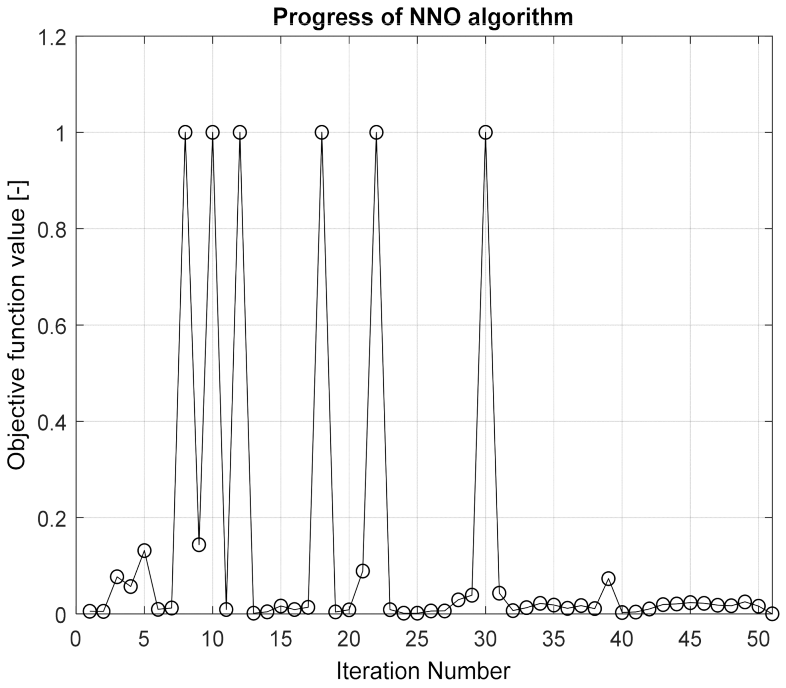
2.3.5. Optimization Procedure

An optimization procedure is carried out to minimize the error between the experimental and the numerical stress strain curve, fANN, subject to the following constraints:
4688 . 43   MPa     E C     4826 . 33   MPa 2757 . 90   MPa     E M     2895 . 80   MPa 0 . 1     ψ     40 0     ε     1 1 . 1     σ b 0 / σ c 0     1 . 2 0 . 51     K c     1 0 . 1     ν M     0 . 4 6 . 89   MPa     σ c 0 , C     41 . 37   MPa 3 . 45   MPa     σ c 0 , M     34 . 47   MPa 10 4     ε tf     10 3
The objective function fANN is a function that accepts any set of design variable values (input data of the ANN) and gives as output the error (output data of the ANN). It is important to note here that as the algorithm proceeds, the training data increases, the trained ANN becomes “better”, and the objective function that is based on this ANN becomes better as well. This means that the objective function changes continuously as the algorithm proceeds, continuously shifting the optimum values of the design variables as well as the objective function.
The gradient based interior point algorithm (IPA) approach is used for the solution of the optimization problem [41]. According to this algorithm, the original inequality constrained minimization problem is stated as follows:
minX{fANN(X)}
subject to:
g ( X ) = LB X X UB     0 0
where X is a vector containing the 10 design variables and LB, UB are also vectors containing the lower and upper bounds of the design variables respectively. Equation (8) is solved as a sequence of the following approximate equality constrained minimization problems for μ > 0:
minX,s{fANN(X,s)} = minX,s{fANN(X)} − μ∑iln(si)
subject to:
g(X) + s = 0
there is one slack variable (si ≥ 0) for each inequality of a design variable, namely the optimization problem at hand has 16 slack variables. As μ decreases to zero, the minimum of [fANN, μ] and the minimum of fANN should coincide.
To solve the approximate problem, the algorithm uses one of the following two main types of steps at each iteration:
  • N Step. A direct (Newton) step in (X,s). This step attempts to solve the Karush Kuhn Tucker (KKT) equations [42,43] for the approximate problem using a linearized Lagrangian as follows:
    H 0 J g T 0 S Λ S J g S I Δ X Δ s Δ λ = f ANN J g T λ S λ     μ e g + s
    where H is the Hessian of the Lagrangian of the approximate equality constrained minimization problem, calculated according to the BFGS formula [44,45,46], Jg is the Jacobian of the inequality constraint function g(X), S is a diagonal matrix with entries si, λ denotes the Lagrange multiplier vector associated with constraints g(X), Λ is a diagonal matrix with entries λi, and e is a vector of ones the same size as g(X). Equation (12) defines the direct step (ΔX, Δs).
  • CG Step. A CG (Conjugate Gradient) step, using a trust region. The conjugate gradient approach to solve the approximate problem, Equation (10) adjusts both X and s, keeping the slacks s positive. The algorithm obtains Lagrange multipliers by approximately solving the KKT equations by:
    XL = ∇XfANN + ∑iλi∇gi(X) = 0
    subject to λ > 0. The following quadratic approximation to Equation (10) is minimized in a trust region of radius R:
    minΔX,Δs{∇fANNTΔX + ½ΔXTXX2LΔX + μeTS−1Δs + ½ΔsTS−1ΛΔs}
    subject to the linearized constraints:
    g(X) + JgΔX + Δs = 0
From Equation (14) the step (ΔX, Δs) is obtained.
By default, the algorithm first attempts to take a direct N step. If it cannot, it attempts a CG step. The algorithm takes a CG step either if the approximate problem is not locally convex near the current iterate, or if the Hessian is not positive definite at the current iteration.
For the first iteration, the initial guess that is supplied to the optimization function corresponds to the best case (i.e., that has the minimum error) among the initial design variable value combinations. For subsequent iterations, the initial guess corresponds to the optimum values that have been obtained in the last iteration of the NNO algorithm.

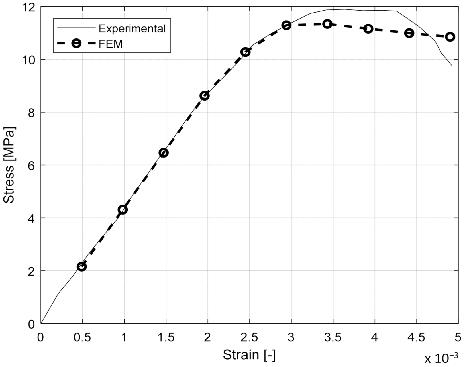
2.3.6. Evaluation of the Stress-Strain Curve of the Optimal Point

An ABAQUS 2021HF5 (6.21-6) analysis is performed in which the material constitutive properties of the prism model are set equal to the optimum solution obtained in the optimization procedure that is described in Section 2.3.5. From the analysis, the stress strain curve is obtained in the same way as outlined in Section 2.3.2. At this step, it is checked if any one of the termination conditions is satisfied. Two termination conditions have been included in the neural optimization algorithm, i.e., if the number of iterations exceeds an upper limit, or if the error becomes lower than a prescribed tolerance:
j > maxIter
err < tol
If any of these two conditions is satisfied, the algorithm terminates and returns as output the best design that is achieved so far (i.e., the design that corresponds to minimum error). If none of the above conditions is satisfied, the last optimum solution is treated as an additional input output training data and is added into the pool of the initial training data. The ANN is retrained based on the enriched training data.

2.4. Material Parameter Identification Results

Figure 4 presents the evolution of the objective function during the inverse optimization procedure. It is obvious that the objective value (i.e., the error) stabilizes after a number of local maxima, as the algorithm proceeds towards its termination point. The oscillating behavior towards convergence depends on the size of the ANN used inside the NNO algorithm (i.e., number and size of hidden layers, etc.). Despite these oscillations, a strongly converging behavior is observed which is indicative of the suitability of the proposed neural optimization algorithm for the solution of inverse optimization problems for model parameter identification. After the optimum calibrated material properties have been obtained, an ABAQUS 2021HF5 (6.21-6) analysis is performed with these properties assigned to the prism model. The numerical stress-strain curve shows a very good agreement with the experimental observation (see Figure 5).

3. Results & Discussion

An essential consideration to assess masonry walls is to examine their resistance against a lateral force caused by wind or earthquake loads. Flexural cracking, shear sliding, and compressive failure are the most common failure modes of the walls under lateral loads. The feasibility of the evaluation process is verified through comparison with corresponding experimental results [1,2,3]. The CDP model is being used to model the mechanical response of mortar layers and bricks in the masonry walls, the material properties of which are based on the optimized CDP material parameters that are obtained from the inverse analysis of the small scale (prism) simulations with the proposed neural optimization algorithm. Moreover, unlike the prism specimens in which the loading is in the vertical direction only, the loading of the URM walls is not only vertical, but also lateral, and for this reason it is assumed that along the brick—mortar interfaces shear failure according to the Mohr-Coulomb shear friction relationship occurs if the shear loading exceeds a certain limit.
The numerical results of the masonry walls regarding the shear stress (τ)—lateral displacement (U) curves showed a good agreement with corresponding experimental observations, as shown in Figure 5 and Figure 6 below.
Next, the model is used to understand failure mechanisms in the masonry walls under lateral loads. The essential aspects that control the flexural cracks in masonry walls are, apart from the material parameters, the wall geometry and the ratio of vertical load to lateral load. Therefore, the effect of different parameters is accounted for by performing a parametric study of load combination and wall aspect ratio l/heff to investigate the crack patterns due to flexural cracking, compressive failure, and sliding shear failure through varying the tensile strength, compressive strength, and coefficient of friction and shear stress on the intact elements between mortar layers and bricks. The ultimate shear strength is determined from the sum of lateral forces at the top nodes of the masonry wall divided by the cross sectional area.

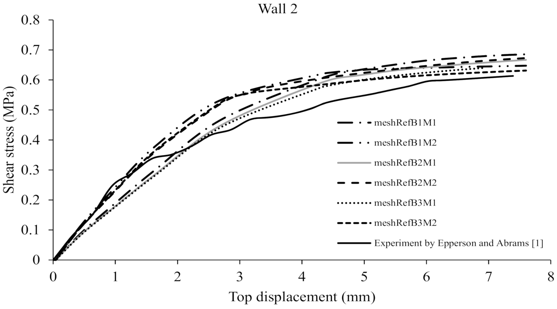
3.1. Mesh Convergence Study

A vital issue in FE simulations that affects accuracy is mesh convergence, namely the mesh refinement that is required, so that the FE solution becomes practically independent of the discretization of the model. Since the geometry of the wall is simple, i.e., without curved geometry, it is obvious that there are not any geometric constraints on the mesh refinement process. The model “Wall 2” [1] is used for the mesh convergence study. This FE model of the URM wall is solved for two levels of refinement for the mortar and three levels of refinement for the bricks. The refinements of the mortar and the bricks are independent, thus they yield six refinement cases, as shown in Table 2. The naming convention of the six models used for the mesh convergence study is meshRefBXMY, where X is the refinement level of the bricks and Y is the refinement level of the mortar. As X and/or Y increase, the refinement increases, i.e., the number of nodes and elements of the FE mesh increase, leading to more accurate solutions. X = 1 corresponds to two finite element discretization along the brick edges. Y = 1 corresponds to one finite element discretization along the thickness of the mortar. For example, in the model meshRefB1M1 all bricks are discretized in two finite elements per edge (i.e., 4 finite elements per brick), and one element along with the mortar thickness. X = 2 and X = 3 correspond to the discretization of three and four elements per edge respectively. Y = 2 corresponds to discretization through the thickness of the mortar in two finite elements. It is noted that the aspect ratio of each finite element of the mortar is equal, or as closest as possible to unity, in order to preserve a good mesh quality. Furthermore, special attention has been paid to ensure that hourglassing and shear locking phenomena do not occur in the FE mesh during the solution process [47]. The number of nodes and elements of the bricks and the mortar of each model is shown in Table 2.
The naming convention of Table 2 is used in the legend of Figure 6, where the shear stress vs. top displacement curves are plotted for the various cases. For reasons of easy comparison, the experimental result has been plotted in Figure 6. It is apparent that the cases with increased mesh refinement are closer to the experimental curve than those with the coarse mesh, which shows that the former cases have increased accuracy. In addition, since the numerical results of the refined mesh are in satisfactory agreement with the experimental results, it is concluded that further refinement of the mesh is not necessary. Therefore, the mesh refinement of the case meshRefB3M2 is used for the parametric analysis the results of which are presented in this study.

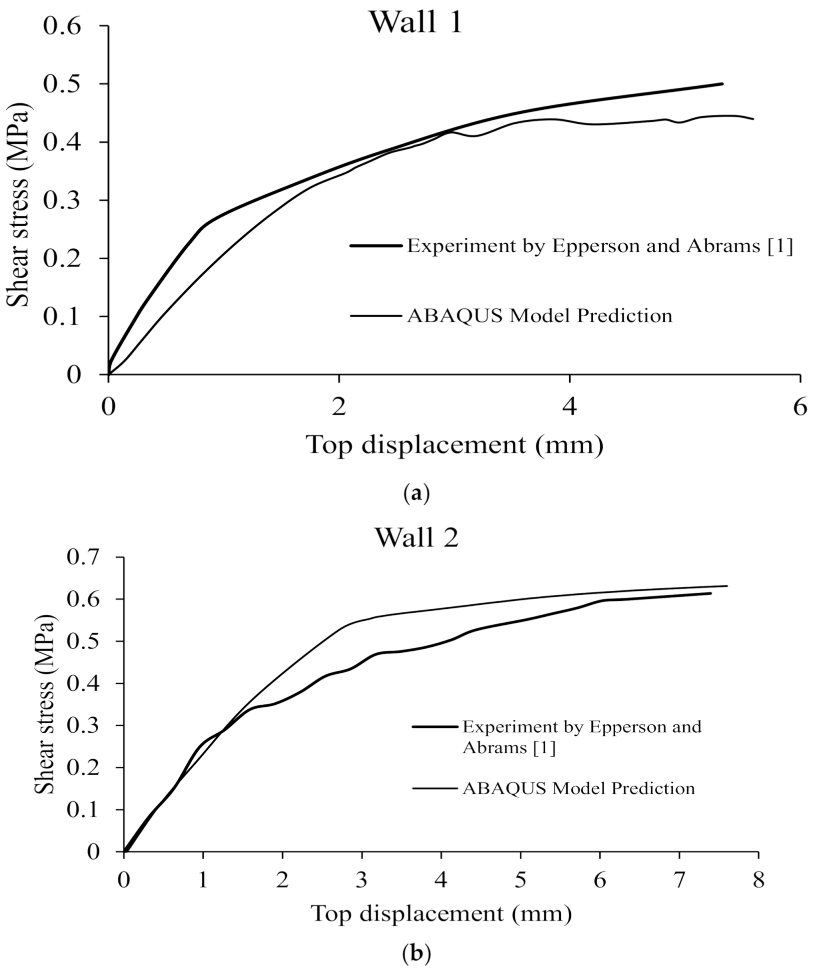
3.2. Model Validation

To check the validity of optimal material parameters obtained from the NNO algorithm for the prism, two URM walls (referred to as “Wall 1” and “Wall 2”) are simulated and compared to experimental tests by Epperson and Abrams [1]. The optimal constitutive parameters of the masonry prism implemented in the numerical simulations of walls are summarized in Table 3. The geometrical model of URM walls is represented by a clay brick panel with the same height of 1828.8 mm height and two different widths 2895.6 mm and 2387.6 mm for “Wall 1” and “Wall 2”, respectively. The cross-section area of “Wall 1” is 1,206,449 mm2 and for “Wall 2” 1,032,256 mm2 which are tested by vertical compressive stress and lateral load displacement. The walls are fixed at their bottom and free at their ends. The ABAQUS 2021HF5 (6.21-6) model of the wall is represented by 2D plane stress elements (CPS8R). The constitutive behavior of both the bricks and the mortar thickness of 19 mm is described by the CDP model. The Poisson ratio of the bricks is equal to 0.2, whereas the Poisson ratio of the mortar is 0.29, obtained according to the results of the inverse optimization analysis presented earlier. The flow potential eccentricity (ε) is equal to 0.61 for both the bricks and the mortar layers, and the ratio of initial equibiaxial compressive yield stress to initial uniaxial compressive yield stress (σb0c0) is set equal to 1.11 for both the bricks and the mortar. The optimal parameters of the masonry prism have been specified in the material definition of the walls, which showed a good agreement with experiment tests (see Figure 7).

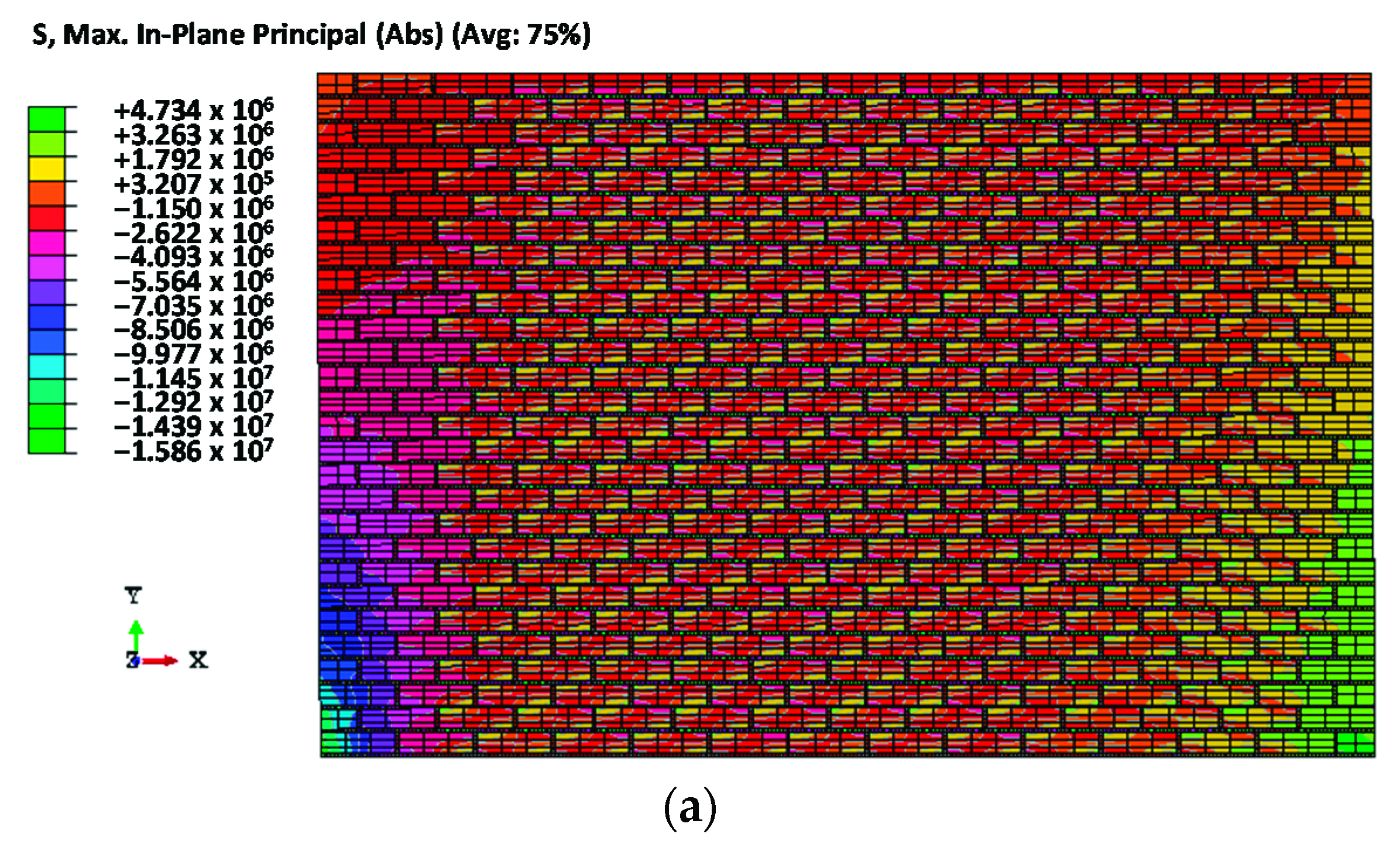
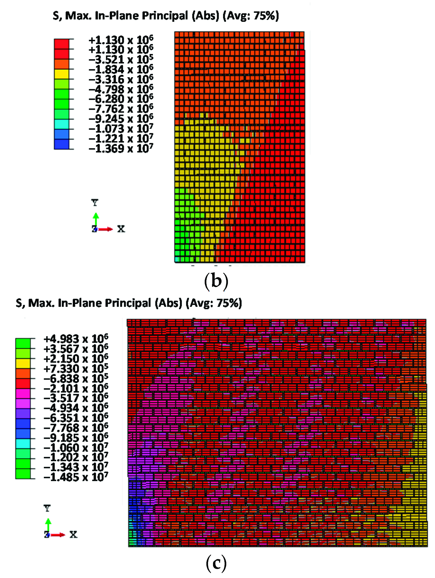
3.3. Failure Modes and Failure Criteria

A parametric study has been conducted to investigate the effect of various factors on the response of URM walls, as outlined in Table 4, and presented in the following sections.

3.3.1. Flexural Cracks

An important parameter in terms of the shear strength of the wall is the flexural tensile strength of the bed joints which can affect the distribution of shear and normal stresses between masonry layers through flexural cracking. Figure 8 shows that the onset of cracking corresponds to the lateral displacement of 2.54 mm which means that the significant deformation begins after 2.54 mm of horizontal displacement. Also, it is obvious that the flexural failure occurs for low vertical compressive stresses σv between 0 to 0.344 MPa combined with high lateral force. Consequently, as the lateral force applied in plane of the wall increases, the inelastic (nonlinear) behavior is more pronounced. As a result, when the flexural tensile cracks extend to the toe of the wall, overturning will occur. Overturning can occur only when the unreinforced wall cracks and the following criterion is used to check failure due to overturning:
τ = ½∙(σv)l/heff

3.3.2. Shear Sliding

The typical shear failure along the bed joint is due to the high lateral forces that cause high shear stress between the bricks and mortar layers. Also, the shear stress between the layers depends on several factors such as the bond between the layers, friction, cohesion, and material heterogeneities. In this study, the friction and cohesion stress between the elements have been investigated. The flexural tensile strength is more important for aspect ratio l/heff = 0.5 with relatively low vertical compressive stress (see Figure 9b). Increasing lateral loads can significantly propagate the crack towards the toe. When the flexural tensile stress exceeds the allowable flexural tensile strength, the cracks propagate near the wall base.
σy ≤ ft
where σy is the tension stress at the base of the wall which is normal to the bed joint and ft is the flexural tensile strength. In general, flexural cracks initiate after the initial stage of the wall response, namely when the horizontal displacement exceeds 2.54 mm. Figure 9a shows failure due to sliding may occur in slender walls with a high aspect ratio l/heff > 1.5 [3]. However, for aspect ratio l/heff = 0.5 shear sliding along the wall length may prevail when it is subjected to high lateral force and low vertical compressive stress. Because the failure can extend over the full width, slender walls are most likely to fail in earlier loading stages compared to stocky walls (see Figure 9b). A major factor that affects this is the bond between brick and mortar layers; for this reason, friction and cohesion stresses have been studied in detail. According to the Mohr-Coulomb shear friction relationship, the shear failure criterion can be stated as follows:
τ ≤ τo + μσy
where τo is the cohesion stress and μ is the coefficient of friction. The latter has been considered in ABAQUS 2021HF5 (6.21-6) software to investigate the effects of the normal and tangential behavior in the contact interfaces between bricks and mortar layers.

3.3.3. Diagonal Compressive Splitting

The diagonal compressive splitting occurs usually when l/heff > 1.5 which is a common failure mechanism, especially when the wall is subjected to high lateral force and vertical compressive stress. Compressive splitting is the last stage before the collapse of the unreinforced walls. In other words, when the wall starts to deflect and a local area of shear sliding starts to form, the diagonal compressive splitting occurs toward the toe causing the wall to overturn. When the URM wall reaches shear sliding failure, redistribution of normal and shear stresses takes place which can be induced from the resultant shear force and can generally delay the collapse event (see Figure 9a). Consequently, toe crashing or diagonal compression splitting may happen due to redistribution of the stresses. Page [48] defined the failure criteria of the biaxial stresses and the principal stresses (σ12) with their orientation θ in terms of 3D surface stresses. These stresses are the normal, tangential, and shear stress to the bed joint, which can be represented by σn, σt, and τ respectively. The failure criteria of biaxial stress is given by:
τ2 ≤ (fmt − σt)(fmn − σn)
where fmt and fmn are the compressive strength at the normal and tangential directions at the bed joints respectively, which can be obtained from masonry prism tests. When the normal stress σn is larger than the compressive strength fmn crushing occurs at the toe [3] (see Figure 9a).

3.3.4. Diagonal Tension Cracking

In this mode, the wall tends to crack at the heel due to high lateral forces and lack of diagonal tensile strength such as seismic loads [49]. This type of failure can occur in the strong brick units and weak mortar which is typically found in walls with aspect ratio l/heff > 1.5. Xu and Abrams [3] stated that strong mortar and weak units cracked with high vertical compressive stresses while weak mortar strong units cracked with low vertical compressive stresses. Essawy and Drysdale [50] presented an equation to determine the principal tensile stress according to Mohr’s circle at a point:
τ σ 0 = 1 σ t σ 0 1 σ n σ 0
where σ0 is the diagonal tension strength in which the diagonal crack occurs when diagonal tensile stress is larger than the diagonal tensile strength.

3.4. Influence of Vertical Compressive Stress

In order to understand the effect of vertical compressive stress, a relationship has been considered between the lateral displacement and shear strength. An aspect ratio l/heff equal to 1.5 is used with compressive strength (f’m) 11 MPa, flexural tensile strength (f’t) 2.06 MPa coefficient of friction (μ) 0.5 and cohesion stress (τo) 0.69 MPa. The values of vertical compressive stress (σv) applied at the top of the walls range from 0.344 MPa to 1.72369 MPa (see Figure 8). The variation of vertical compressive stress can significantly affect the failure mode. When low vertical compressive stress is applied at the top of a slender wall with high lateral loads, the shear sliding may predominate the failure modes. The wall with aspect ratio l/heff = 0.5 is more likely to fail by sliding due to its short length. The effect of vertical compressive stress on the shear strength is slightly increased after the shear sliding modes start to propagate between the brick units and bed joints. Consequently, the shear stress is redistributed in some local areas in the normal and tangential directions that can increase the shear strength till a compression failure is reached. The URM wall with lateral displacement between 0 to 20.32 mm exhibits elastic behavior while nonlinear behavior takes place as soon as the wall starts cracking.

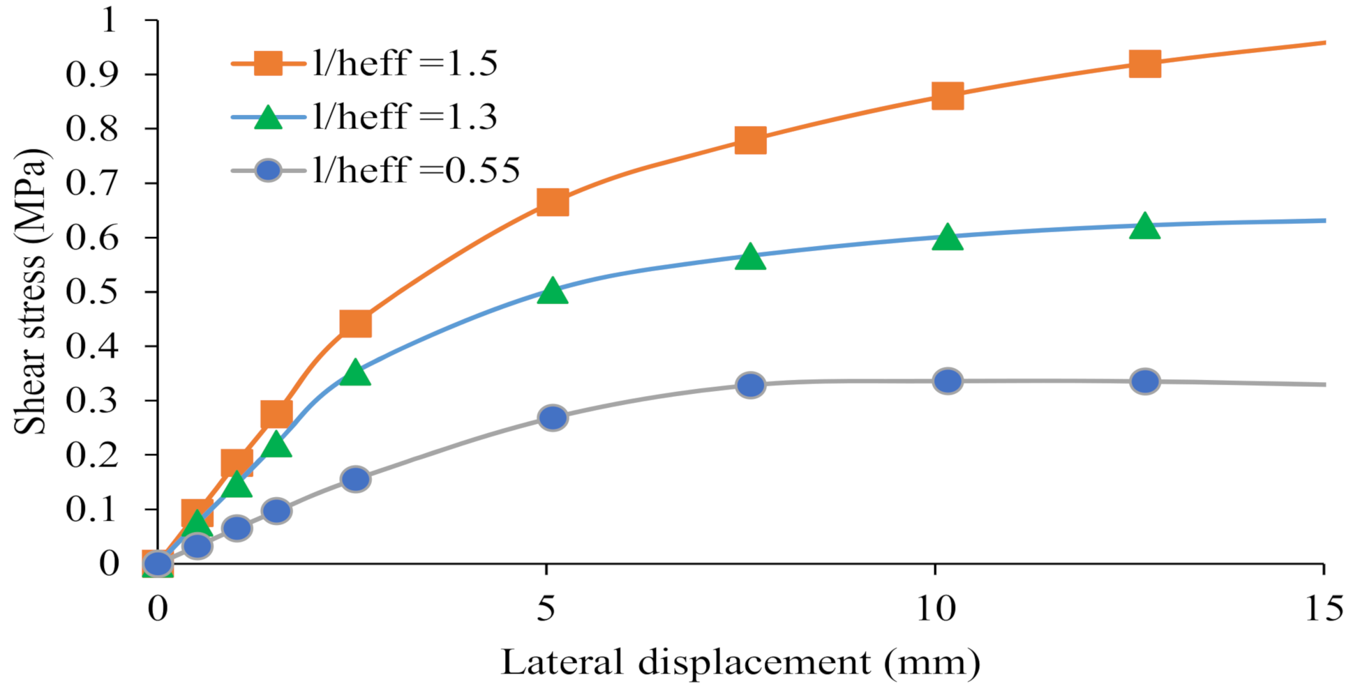
3.5. Influence of Aspect Ratio

In this section, the relationship between the lateral shear load displacement and shear strength is investigated in terms of the length to effective height (aspect) ratio l/heff. The shear strength is estimated from the summation of lateral forces, due to the imposed displacement (ranging from 0 up to 15.24 mm) at the top nodes of the masonry walls divided by their gross sectional area. The vertical compressive stress, flexural tensile strength, and compressive strength are specified equal to 1.03 MPa, 2.06 MPa, and 20.69 MPa respectively. The friction coefficient and cohesion stress are equal to 0.7 and 1.03 MPa respectively. The aspect ratio is the only parameter that is varied to investigate the effect shear strength capacity (e.g., 0.55, 1.3 and 1.6). The shear strength resistance increases significantly when l/heff increases (see Figure 10) [3]. The common failure mechanisms are flexural cracking, shear sliding and compressive splitting which occur in sequence. The higher the aspect ratio, the more failure modes show up during high lateral loads combined with low vertical compression stress [26]. When the aspect ratio is l/heff > 1.5, most failure modes occur during high lateral loading (e.g., rocking, bed joint sliding, diagonal tension splitting and toe crush) (see Figure 9a). The sequence of this failure started with cracks usually near the wall base which then propagate across the wall [49]. Then, the wall started unbinding between the brick units and mortar layers in which this stage may extend across the wall length especially with l/heff < 1.5 (see Figure 9b,c). Shear sliding can play a significant role to redistribute the normal and tangential stresses between the bed joints and brick units. Consequently, the propagation of shear sliding forms a typical stair stepped bed joint that can enhance a ductile mode with significant hysteretic energy dissipation capability. Masonry walls with 0.5 < l/heff < 1.5 may show all failure mechanisms except rocking foundation during high loads (See Figure 9c).

3.6. Influence of Material Sensitivity

In order to investigate the effects of material parameters sensitivity, a relationship between lateral displacement and shear strength has been constructed for URM walls. The shear strength of a cracked wall is calculated by the maximum in-plane lateral force divided by the gross sectional area, i.e., from the sum of lateral force of the top nodes divided by the gross sectional area. The masonry wall is simulated in ABAQUS 2021HF5 (6.21-6) with dimensions of 1.83 m height and 2895.6 mm length and its gross area is 1,206,449 mm2. The wall is subjected to an in-plane lateral load displacement [26], starting from 0 up to 15.24 mm. The CDP model is used with the material parameters that have been used for the verification of the wall response in Section 3.1. In order to understand the post cracking behavior, it is essential to carry out parametric studies, the parameters of which are the compressive strength, the coefficient of friction and the cohesion between the bricks and mortar layers [1,2,3].

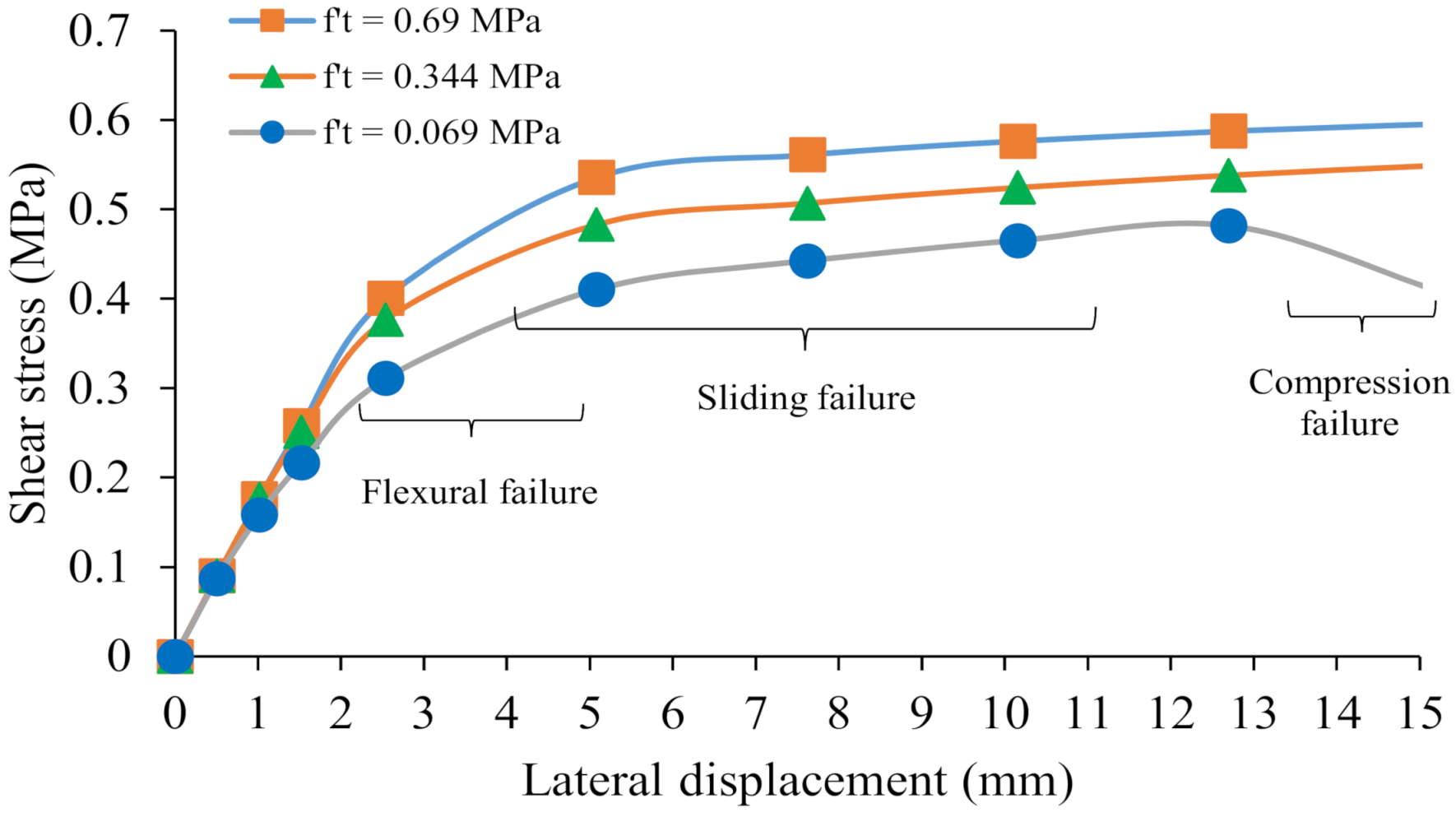
3.6.1. Flexural Tensile Strength

Flexural tensile strength is the most important factor which contributes to the shear resistance and controls the ductility when the masonry walls are subject to in-plane lateral loads. The low vertical compressive stress and high lateral displacement can significantly affect slender walls. In order to investigate the flexural shear strength, the relationship between the lateral displacement and shear strength is considered [3]. The aspect ratio is 1.5 with 11. MPa as compressive strength and coefficient friction and cohesion stress are equal to 0.7 and 0.69 MPa respectively. Flexural tensile strength (f’t) is the only parameter that is varied (e.g., 0.069 MPa, 0.344 MPa, and 0.69 MPa) to evaluate the shear strength. Figure 11 shows that for higher flexural tensile strength, the masonry wall’s resistance to the lateral loads and ductility increase. For lateral displacement equal to 20.32 mm flexural cracks begin to propagate [3]. In addition, when the wall is subjected to lateral load displacement equal to 12.7 mm, it fails with 0.069 MPa of flexural tensile strength. Also, the shear sliding failure predominates in the failure stage as illustrated in Figure 11 compared to other failure stages. Consequently, the shear sliding between the bed joints increases the resistance against collapse as well as ductility.

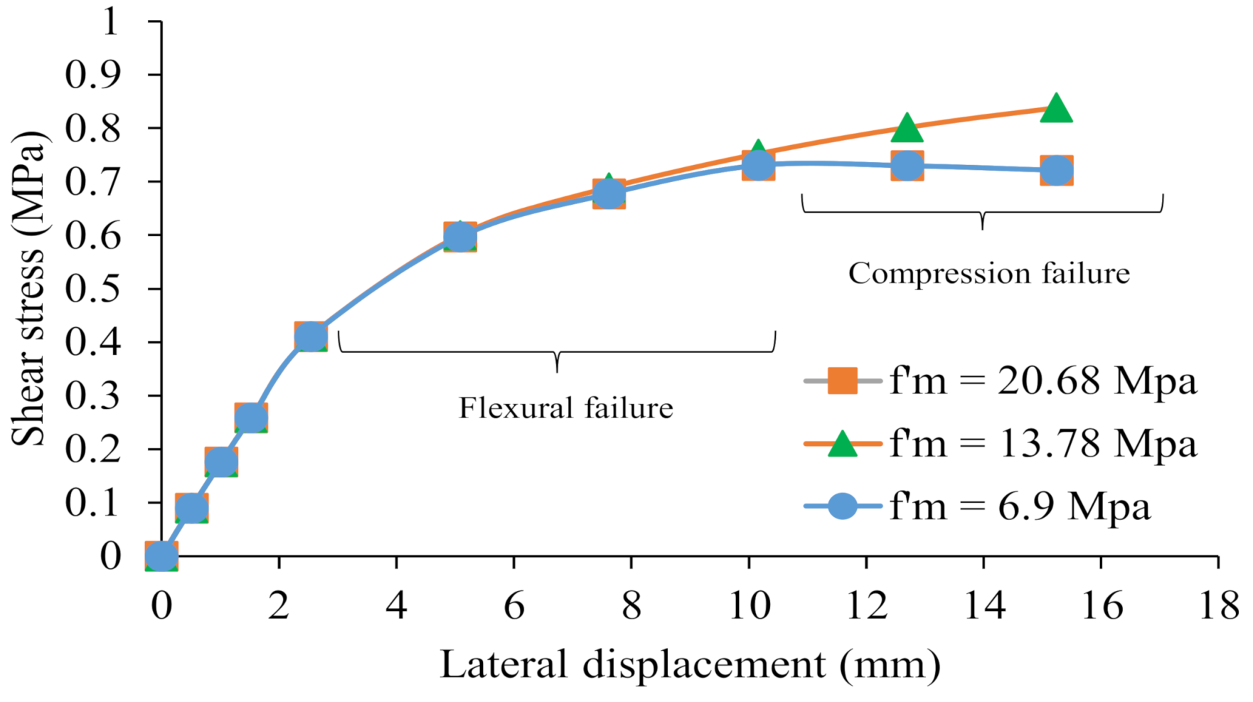
3.6.2. Compressive Strength

Compressive strength is an important parameter that controls failure due to vertical compressive stresses. Three values for compressive strength (f′m) have been considered in the simulation (e.g., 6.9 MPa, 13.8 MPa, and 20.68 MPa). The vertical compressive stress is equal to 1.03 MPa for masonry wall, l/heff = 1.5 and the other parameters are as follows: flexural tensile strength 2.07 MPa, cohesion stress 1.03 MPa and coefficient of friction 0.7. However, when the compressive strength is equal to 6.9 MPa, the strength of the wall is significantly reduced, and it fails at lateral load displacement equal to 10.16 mm (see Figure 12). From Figure 12 it is noted that flexural cracks are created when the lateral displacement ranges from 2.54 mm to 5.08 mm and the shear sliding ranges between 5.08 mm and 10.16 mm and then compressive splitting takes place until collapse. The variation of compressive strength demonstrates clearly that all curves start in the same range of flexural cracking and shear sliding whereas the compressive splitting controls the shear strength. Consequently, if the wall does not fail due to the compressive stress, then the shear strength of the wall does not depend on the compressive strength [3,4].

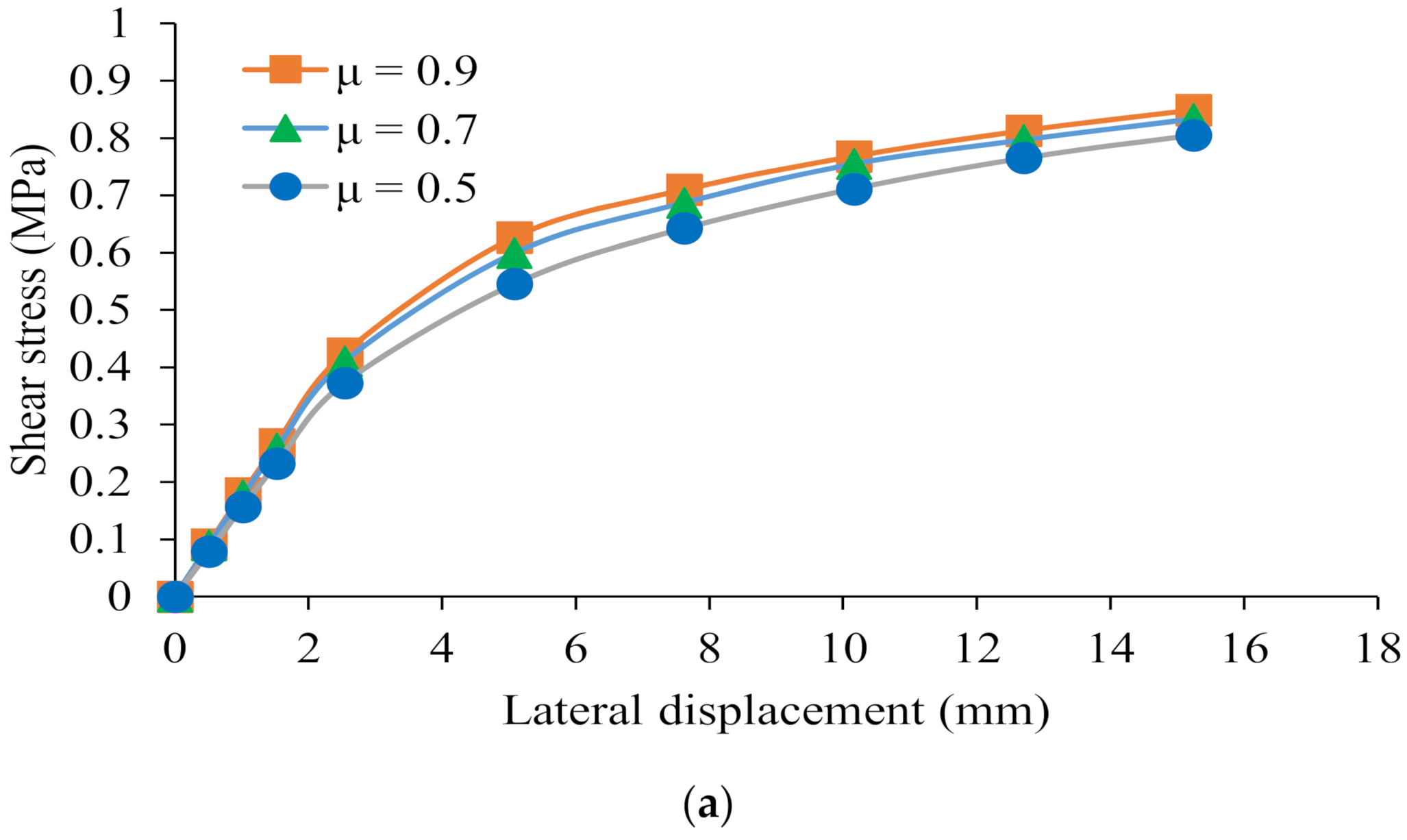
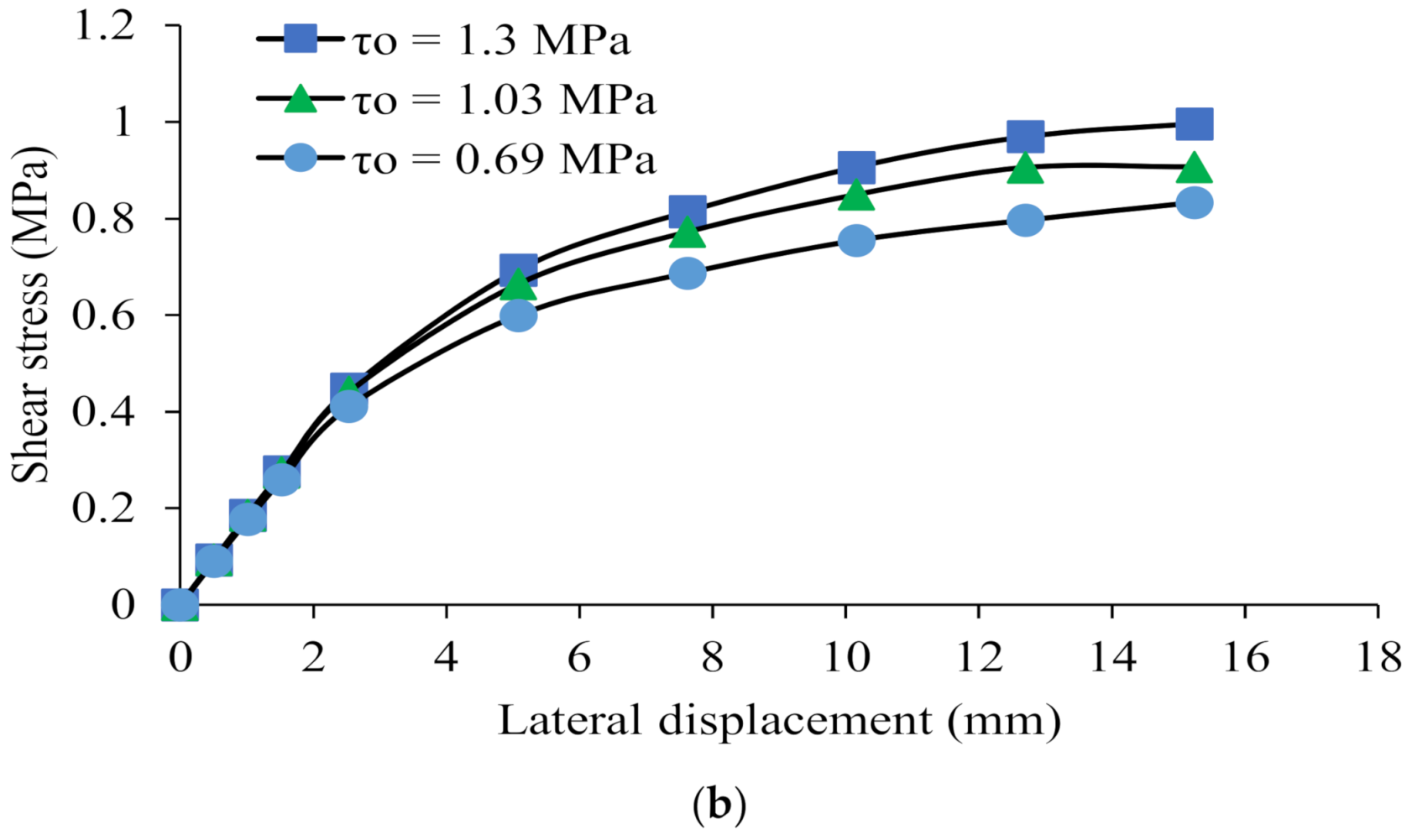
3.6.3. Coefficient of Friction and Cohesion Stress

Coefficient of friction (μ) and cohesion stress (τo) depend on the normal and tangential behavior between the brick units and mortar layers. The Mohr Coulomb criterion in Equation (20) shows that friction and cohesion significantly affect the shear sliding failure. As these two parameters increase, the shear strength to resist shear sliding failure that propagates along the length of masonry wall increases (see Figure 13a). When the applied lateral load is low, the variation of the shear strength is slightly changed with respect to high coefficient of friction and cohesion stress [3]. Consequently, in most cases the region of sliding failure varies based on the local values of normal and tangential stresses between the bed joints [49]. To investigate the variation effect of coefficient of friction and cohesion stress, URM walls are individually simulated corresponding to parameters and aspect ratio similar to those mentioned above, except for coefficient of friction and cohesion stress, which take the values [0.5, 0.7, 0.9] and [0.69 MPa, 1.03 MPa, 1.37 MPa], respectively. The result is a slightly change in shear strength from 0.7 to 0.9 while the coefficient of friction is more sensitive for values from 0.5 to 0.7. Consequently, for higher values of the friction coefficient, less variation of shear strength can be achieved. The variation of cohesion significantly controls the shear strength when the wall is subjected to in-plane lateral loads.
For lower values of cohesion stress the effect on the shear strength becomes more pronounced. Figure 13b illustrates that shear sliding begins earlier for cohesion equal to 0.69 MPa compared to the other cohesion values.

4. Conclusions

A novel Neural Network Optimization (NNO) algorithm has been proposed for the calibration of the material properties of URM walls based on experimental stress—strain curves taken from wall prism compression tests. The calibrated material properties that are output from this algorithm have been used in large scale URM wall FE models the results of which agree very well with analogous experimental data from large scale URM walls. Consequently, it is concluded that the proposed NNO algorithm is able to calibrate the brick and mortar material properties for large scale URM walls, by using experimental results only from wall prism tests, without the necessity for performing costly large scale URM wall experimental tests. This advantage makes the proposed methodology not only cost effective, but also it shows that the NNO concept yields a sufficiently robust and accurate inverse optimization technique for the development of numerical models based on inverse analysis of experimental data.
Apart from this, based on the material properties calibrated with the proposed NNO algorithm, various FE models of large scale URM walls have been developed and the influence of various factors on their shear response is investigated. It has been found that the shear stress is redistributed in some local areas in the normal and tangential directions that can increase the shear strength till a compression failure is reached. Shear sliding can play a significant role to redistribute the normal and tangential stresses between the bed joints and brick units. Consequently, the propagation of shear sliding forms a typical stair stepped bed joint that can enhance a ductile mode with significant hysteretic energy dissipation capability. Generally, the shear sliding between the bed joints increases the resistance against collapse as well as the ductility of the wall.
The application of the proposed calibration strategy to estimate the response of URM walls based on the experimental response of a mesoscale model has shown some critical issues, and treating them in future studies may lead to substantial improvements regarding the implementation of the proposed algorithm. Apart from this, the proposed algorithm can be applied for constitutive calibration in more complicated URM wall structural response, which in turn requires increasingly complex constitutive and numerical models, or can be applied even for predicting the response of other types of loading and/or materials, e.g., interface elements, mortars, bricks, out-of-plane loading of URM walls, etc. Given this broad scope of applications of the proposed NNO algorithm and its mixed AI-gradient nature, it is obvious that future research is needed to improve both its programmatical implementation and its applications in practical engineering problems, as already mentioned above.

Author Contributions

Conceptualization, Q.A.-J. and G.P.; methodology, Q.A.-J. and G.P.; software, G.P.; validation, Q.A.-J.; formal analysis, Q.A.-J.; resources, Q.A.-J.; writing—original draft preparation, Q.A.-J.; writing—review and editing, G.P. All authors have read and agreed to the published version of the manuscript.

Funding

This research received no external funding.

Institutional Review Board Statement

Not applicable.

Informed Consent Statement

Not applicable.

Data Availability Statement

The data presented in this study are available upon request from the corresponding author.

Conflicts of Interest

The authors declare no conflict of interest.

Appendix A. Literature Review Summary

ReferencesKeywordsFinding
[1,2,3,4]Masonry Walls, Shear strength evaluation, Nondestructive evaluation(a) Determine of vertical compressive stress for masonry walls subjected to in-plane lateral loads.
(b) Conducted paramteric study to evalute shear strength.
[5,6,7,8,9,10,11]Concrete damage plasticity CDP, Constitutive model(a) Developed concrete damage plasticity constititve mode and validated with numerical/experiment data.
(b) Calibrate material parameters and validated with experimental observations.
[12,13,14,15,16,17,18,19,20,21,22,23]Parameters Identification, FE, Calibration, OptimizationStudy masonry mesoscale/macroscale model subjected to load combination and compared its results with those of a finite element (FE) model to identify the material parameters.
[24,25,26,27]Masonry walls, strength evaluation, Aspect ratioInvestigate the effects of various factors, i.e., unit type, vertical pre compression level, aspect ratio, size, and boundary conditions, on the displacement capacity of URM walls.
[28,29,30,31]Optimization, Calibration, Material parameters identificationCalibrate masonry model, characterize the material parameters based on experimental observations
[32,33]Optimization, Least squares, Material parametersOptimization algorithm to minimize the errors of the differences between experiment-based measurements and the calculated response of the model.

References

  1. Epperson, G.S.; Abrams, D.P. Nondestructive Evaluation of Masonry Buildings; University of Illinois at Urbana-Champaign: Champaign, IL, USA, 1990; Volume 89. [Google Scholar]
  2. Abrams, D.P.; Shah, N. Cyclic Load Testing of Unreinforced Masonry Walls; Illinois Univ at Urbana Advanced Construction Technology Center: Champaign, IL, USA, 1992. [Google Scholar]
  3. Xu, W.; Abrams, D.P. Evaluation of Lateral Strength and Deflection for Cracked Unreinforced Masonry Walls; Illinois Univ at Urbana Advanced Construction Technology Center: Champaign, IL, USA, 1992. [Google Scholar]
  4. Chaimoon, K.; Attard, M.M. Modeling of unreinforced masonry walls under shear and compression. Eng. Struct. 2007, 29, 2056–2068. [Google Scholar] [CrossRef]
  5. Lotfi, H.; Shing, P. An appraisal of smeared crack models for masonry shear wall analysis. Comput. Struct. 1991, 41, 413–425. [Google Scholar] [CrossRef]
  6. Grassl, P.; Jirásek, M. Damage-plastic model for concrete failure. Int. J. Solids Struct. 2006, 43, 7166–7196. [Google Scholar] [CrossRef] [Green Version]
  7. Lubliner, J. A simple model of generalized plasticity. Int. J. Solids Struct. 1991, 28, 769–778. [Google Scholar] [CrossRef]
  8. Lubliner, J.; Oliver, J.; Oller, S.; Oñate, E. A plastic-damage model for concrete. Int. J. Solids Struct. 1989, 25, 299–326. [Google Scholar] [CrossRef]
  9. Gambarotta, L.; Lagomarsino, S. Damage models for the seismic response of brick masonry shear walls. Part I: The mortar joint model and its applications. Earthq. Eng. Struct. Dyn. 1997, 26, 423–439. [Google Scholar] [CrossRef]
  10. Kmiecik, P.; Kamiński, M. Modelling of reinforced concrete structures and composite structures with concrete strength degradation taken into consideration. Arch. Civ. Mech. Eng. 2011, 11, 623–636. [Google Scholar] [CrossRef]
  11. Lee, J.; Fenves, G.L. Plastic-damage model for cyclic loading of concrete structures. J. Eng. Mech. 1998, 124, 892–900. [Google Scholar] [CrossRef]
  12. Chisari, C.; Macorini, L.; Amadio, C.; Izzuddin, B.A. Identification of mesoscale model parameters for brick-masonry. Int. J. Solids Struct. 2018, 146, 224–240. [Google Scholar] [CrossRef]
  13. Chisari, C. Inverse Techniques for Model Identification of Masonry Structures; Università degli studi di Trieste: Trieste, Italy, 2015. [Google Scholar] [CrossRef] [Green Version]
  14. Chisari, C.; Macorini, L.; Amadio, C.; Izzuddin, B. An inverse analysis procedure for material parameter identification of mortar joints in unreinforced masonry. Comput. Struct. 2015, 155, 97–105. [Google Scholar] [CrossRef] [Green Version]
  15. Chisari, C. Tolerance-based Pareto optimality for structural identification accounting for uncertainty. Eng. Comput. 2019, 35, 381–395. [Google Scholar] [CrossRef] [Green Version]
  16. Caliò, I.; Marletta, M.; Pantò, B. A new discrete element model for the evaluation of the seismic behaviour of unreinforced masonry buildings. Eng. Struct. 2012, 40, 327–338. [Google Scholar] [CrossRef]
  17. Carmeliet, J. Optimal estimation of gradient damage parameters from localization phenomena in quasi-brittle materials. Mech. Cohesive-Frict. Mater. Int. J. Exp. Model. Comput. Mater. Struct. 1999, 4, 1–16. [Google Scholar] [CrossRef]
  18. Muñoz-Rojas, P.; Cardoso, E.; Vaz, M. Parameter identification of damage models using genetic algorithms. Exp. Mech. 2010, 50, 627–634. [Google Scholar] [CrossRef]
  19. Nazari, A.; Sanjayan, J.G. Modelling of compressive strength of geopolymer paste, mortar and concrete by optimized support vector machine. Ceram. Int. 2015, 41, 12164–12177. [Google Scholar] [CrossRef]
  20. Toropov, V.V.; van der Giessen, E. Parameter identification for nonlinear constitutive models: Finite Element simulation—Optimization—Nontrivial experiments. In Optimal Design with Advanced Materials; Elsevier: Amsterdam, The Netherlands, 1993; pp. 113–130. [Google Scholar]
  21. Sarhosis, V.; Sheng, Y. Identification of material parameters for low bond strength masonry. Eng. Struct. 2014, 60, 100–110. [Google Scholar] [CrossRef] [Green Version]
  22. Jankowiak, T.; Lodygowski, T. Identification of parameters of concrete damage plasticity constitutive model. Found. Civ. Environ. Eng. 2005, 6, 53–69. [Google Scholar]
  23. Toropov, V.; Garrity, S. Material parameter identification for masonry constitutive models. In Proceedings of the Eighth Canadian Masonry Symposium, Jasper, AB, Canada, 31 May–3 June 1998; pp. 551–562. [Google Scholar]
  24. Magenes, G.; Calvi, G.M. In-plane seismic response of brick masonry walls. Earthq. Eng. Struct. Dyn. 1997, 26, 1091–1112. [Google Scholar] [CrossRef]
  25. Agnihotri, P.; Singhal, V.; Rai, D.C. Effect of in-plane damage on out-of-plane strength of unreinforced masonry walls. Eng. Struct. 2013, 57, 1–11. [Google Scholar] [CrossRef]
  26. Salmanpour, A.H.; Mojsilović, N.; Schwartz, J. Displacement capacity of contemporary unreinforced masonry walls: An experimental study. Eng. Struct. 2015, 89, 1–16. [Google Scholar] [CrossRef]
  27. Howlader, M.K.; Masia, M.; Griffith, M. Numerical analysis and parametric study of unreinforced masonry walls with arch openings under lateral in-plane loading. Eng. Struct. 2020, 208, 110337. [Google Scholar] [CrossRef]
  28. Labibzadeh, M.; Zakeri, M.; Shoaib, A.A. A new method for CDP input parameter identification of the ABAQUS software guaranteeing uniqueness and precision. Int. J. Struct. Integr. 2017, 8, 264–284. [Google Scholar] [CrossRef]
  29. Birtel, V.; Mark, P. Parameterised finite element modelling of RC beam shear failure. In Proceedings of the 2006 ABAQUS Users’ Conference, Boston, MA, USA, 23–25 May 2006; Volume 14. [Google Scholar]
  30. Levenberg, K. A method for the solution of certain non-linear problems in least squares. Q. Appl. Math. 1944, 2, 164–168. [Google Scholar] [CrossRef] [Green Version]
  31. Albu Jasim, Q.J.M. Probabilistic Calibration of Unreinforced Masonry Wall Properties: From Constitutive Material Models to Structural Performance. Ph.D. Thesis, Texas A & M University, College Station, TX, USA, 2020. [Google Scholar]
  32. Simulia, D. Abaqus Version 2021HF5 (6.21-6) Documentation USA; Dassault Systemes Simulia Corporation: Johnston, RI, USA, 2021. [Google Scholar]
  33. MATLAB. R2021a; MathWorks Inc.: Natick, MA, USA, 2021. [Google Scholar]
  34. Papazafeiropoulos, G.; Muñiz-Calvente, M.; Martínez-Pañeda, E. Abaqus2Matlab: A suitable tool for finite element post-processing. Adv. Eng. Softw. 2017, 105, 9–16. [Google Scholar] [CrossRef] [Green Version]
  35. Marquardt, D.W. An algorithm for least-squares estimation of nonlinear parameters. J. Soc. Ind. Appl. Math. 1963, 11, 431–441. [Google Scholar] [CrossRef]
  36. Foresee, F.D.; Hagan, M.T. Gauss-Newton approximation to Bayesian learning. In Proceedings of the International Conference on Neural Networks (ICNN’97), Houston, TX, USA, 12 June 1997; pp. 1930–1935. [Google Scholar] [CrossRef]
  37. Byrd, R.H.; Gilbert, J.C.; Nocedal, J. A trust region method based on interior point techniques for nonlinear programming. Math. Program. 2000, 89, 149–185. [Google Scholar] [CrossRef] [Green Version]
  38. Byrd, R.H.; Hribar, M.E.; Nocedal, J. An interior point algorithm for large-scale nonlinear programming. SIAM J. Optim. 1999, 9, 877–900. [Google Scholar] [CrossRef]
  39. MacKay, D.J. Bayesian interpolation. Neural Comput. 1992, 4, 415–447. [Google Scholar] [CrossRef]
  40. Waltz, R.A.; Morales, J.L.; Nocedal, J.; Orban, D. An interior algorithm for nonlinear optimization that combines line search and trust region steps. Math. Program. 2006, 107, 391–408. [Google Scholar] [CrossRef]
  41. Karush, W. Minima of Functions of Several Variables with Inequalities as Side Constraints. Master’s thesis, The University of Chicago, Chicago, IL, USA, 1939. [Google Scholar]
  42. Kuhn, H.; Tucker, A. Nonlinear Programming. In Proceedings of the Second Berkeley Symposium on Mathematical Statistics and Probability, Berkeley, CA, USA, 31 July–12 August 1950. [Google Scholar]
  43. Broyden, C.G. The convergence of a class of double-rank minimization algorithms 1. general considerations. IMA J. Appl. Math. 1970, 6, 76–90. [Google Scholar] [CrossRef]
  44. Fletcher, R. A new approach to variable metric algorithms. Comput. J. 1970, 13, 317–322. [Google Scholar] [CrossRef] [Green Version]
  45. Goldfarb, D. A family of variable-metric methods derived by variational means. Math. Comput. 1970, 24, 23–26. [Google Scholar] [CrossRef]
  46. Shanno, D.F. Conditioning of quasi-Newton methods for function minimization. Math. Comput. 1970, 24, 647–656. [Google Scholar] [CrossRef]
  47. Reddy, J.N. An Introduction to Nonlinear Finite Element Analysis: With Applications to Heat Transfer, Fluid Mechanics, and Solid Mechanics; Oxford University Press: New York, NY, USA, 2015. [Google Scholar] [CrossRef]
  48. Page, A. The biaxial compressive strength of brick masonry. Proc. Inst. Civ. Eng. 1981, 71, 893–906. [Google Scholar] [CrossRef]
  49. Agency, F.E.M. Evaluation of Earthquake Damaged Concrete and Masonry Wall Buildings; FEMA: Washington, DC, USA, 2013.
  50. Essawy, A.S.; Drysdale, R.G. Macroscopic failure criterion for masonry assemblages. In Proceedings of the 4th Canadian Masonry Symposium, Fredericton, NB, Canada, 2–4 June 1986; Volume 1, pp. 263–277. [Google Scholar]
Figure 1. Flowchart of the steps implemented in the Section 3 of the present study.
Civileng 02 00051 g001
Figure 2. Numerical model of 3D prism considered for the parameter identification in this study.
Civileng 02 00051 g002
Figure 3. Architecture of the feedforward ANN with backpropagation that is used in the present study.
Civileng 02 00051 g003
Figure 4. Evolution of the objective function during the NNO process.
Civileng 02 00051 g004
Figure 5. Stress strain experimental observation vs. FE model prediction.
Civileng 02 00051 g005
Figure 6. Mesh convergence results for the model “Wall 2”.
Civileng 02 00051 g006
Figure 7. Experimental and numerical shear stress versus top displacement curves: (a) model “Wall 1”, (b) model “Wall 2”.
Civileng 02 00051 g007
Figure 8. Influence of compressive vertical stress on shear strength of URM walls. Xu and Abrams [3] presented an equation to evaluate the cracking of unreinforced walls due to flexural tensile stress τ = ⅙ l/heff(ft + σv) where τ is the nominal shear stress between the brick and mortar layers.
Civileng 02 00051 g008
Figure 9. URM wall simulations in ABAQUS for validation of the various failure mechanisms: (a) stocky, (b) slender and (c) square.
Civileng 02 00051 g009aCivileng 02 00051 g009b
Figure 10. Influence of aspect ratio in shear strength of URM walls.
Civileng 02 00051 g010
Figure 11. Influence of flexural tensile strength on shear strength of URM walls.
Civileng 02 00051 g011
Figure 12. Influence of compressive strength on shear strength of URM walls.
Civileng 02 00051 g012
Figure 13. Influence of contact properties on shear strength of URM walls: (a) friction, (b) cohesion.
Civileng 02 00051 g013aCivileng 02 00051 g013b
Table 1. Description and bounds of the design variables considered for fitting the experimental stress strain curve of the prism.
Design VariableDescriptionLower BoundUpper Bound
ECModulus of elasticity of the brick material4688.43 MPa4826.33 MPa
EMModulus of elasticity of the mortar material2757.90 MPa2895.80 MPa
ψDilation angle in the p–q plane of the brick material0.140
εFlow potential eccentricity01
σb0c0Ratio of initial equibiaxial compressive yield stress to initial uniaxial compressive yield stress 1.11.2
KcRatio of the second stress invariant on the tensile meridian to that on the compressive meridian at initial yield0.511
νMPoisson ratio of the mortar material0.10.4
σc0,CInitial yield stress value of brick material in compression for crushing strain equal to 0.06.89 MPa41.37 MPa
σc0,MInitial yield stress value of mortar material in compression, for crushing strain equal to 0.03.45 MPa34.47 MPa
εtfCracking strain in tension, for failure stress value equal to 1/10 of the failure stress value for cracking strain equal to 0.010−410−3
Table 2. Modeling details of the 6 simulation cases used for the mesh refinement study.
ModelPartElement TypeElementsNodes
meshRefB1M1MortarCPS4R10,10819,570
BricksCPS4R15683528
meshRefB1M2MortarCPS4R34,94150,822
BricksCPS4R15683528
meshRefB2M1MortarCPS4R10,10819,570
BricksCPS4R35286272
meshRefB2M2MortarCPS4R34,94150,822
BricksCPS4R35286272
meshRefB3M1MortarCPS4R10,10819,570
BricksCPS4R62729800
meshRefB3M2MortarCPS4R34,94150,822
BricksCPS4R62729800
Table 3. Optimal material properties of the small scale wall prism.
Design VariableOptimum Value
EC4744.97 MPa
EM2819.13 MPa
ψ8.88
ε0.61
σb0c01.112
Kc0.84
νM0.294
σc0,C15.547 MPa
σc0,M9.067 MPa
ε t f 1.01 × 10⁻⁴
Table 4. Classification of parameters and models in the parametric study of URM walls carried out in this study (see footnote after the table for the conclusion statements).
DescriptionConstant InputVarying InputOutputsConclusion
Shear Stress (τ)
MPa
Lateral Dis (U) mm
Influence of Vertical Compressive Stressl/heff = 1.5
f’m = 11 MPa
μ = 0.5
τo = 0.69 MPa.
f’t = 2.06 MPa
σv = 0.344 MPa
σv = 0.69 MPa
σv = 1.03 MPa
σv = 1.37 MPa
σv = 1.72 MPa
(0.72) a
(0.78) a
(0.83) a
(0.88) a
(0.91) a
(15.24) b
(15.24) b
(15.24) b
(15.24) b
(15.24) b
Note 1
Influence of Aspect Ratiof’m = 20.69 MPa
μ = 0.5
τo = 0.69 MPa.
σv = 1.03 MPa
f’t = 2.06 MPa
l/heff = 0.55
l/heff = 1.3
l/heff = 1.5
(0.32) a
(0.63) a
(0.96) a
(15.24) b
(15.24) b
(15.24) b
Note 2
Influence of Material Sensitivity: Flexural Tensile Strengthl/heff = 1.5
μ = 0.5
τo = 0.69 MPa
σv = 1.03 MPa
f’m = 11 MPa
f’t = 0.069 MPa
f’t = 0.344 MPa
f’t = 0.69 MPa
(0.40) a
(0.54) a
(0.59) a
(15.24) b
(15.24) b
(15.24) b
Note 3
Influence of Material Sensitivity: Compressive Strengthl/heff = 1.5
μ = 0.5
τo = 0.69 MPa
σv = 1.03 MPa
f’t = 2.06 MPa
f’m = 6.9 MPa
f’m = 13.78 MPa
f’m = 20.68 MPa
(0.72) a
(0.83) a
(0.72) a
(15.24) b
(15.24) b
(15.24) b
Note 4
Influence of Material Sensitivity: Coefficient of Frictionl/heff = 1.5
f’m = 11 MPa
τo = 0.69 MPa.
σv = 1.03 MPa
f’t = 2.06 MPa
μ = 0.5
μ = 0.7
μ = 0.9
(0.80) a
(0.83) a
(0.85) a
(15.24) b
(15.24) b
(15.24) b
Note 5
Influence of Material Sensitivity: Cohesion Stressl/heff = 1.5
f’m = 11 MPa
μ = 0.5
σv = 1.03 MPa
f’t = 2.06 MPa
τo = 0.69 MPa.
τo = 1.03 MPa.
τo = 1.3 MPa
(0.83) a
(0.90) a
(0.99) a
(15.24) b
(15.24) b
(15.24) b
a Represent the shear stress values when wall b lateral displacement reaches to 15.24 mm. Note 1: By assuming increasing vertical compressive stress the failure mode from flexural to compressive splitting exhibited in Figure 8. With high vertical compressive stress, fail in flexure may occur quickly towards the toe due to flexural cracking progresses in bed joint. Note 2: Wall with l/heff > 1.3, the failure is primarily a result of compressive splitting from flexure and compressive splitting. Slender wall fails in bed joint due to the flexural cracks or local sliding. Note 3: The flexural tensile strength significantly influences on the lateral stress that instigates cracking. As a result, the more the flexural tensile strength, the more the shear capacity for flexural cracking failure. Note 4: The shear strength is dominated by the compressive strength when the wall is investigated for the compression failure mode. If the wall fails in compression, this means the shear strength depends on the compression strength. Note 5: The variations for cohesion and coefficient of friction values may cause slide failure at different vertical stress level. In consequence, the compressive strength failure may occur in some local area due to the lack of bond between the mortar and brick units.
Publisher’s Note: MDPI stays neutral with regard to jurisdictional claims in published maps and institutional affiliations.

