
Assessing the Capability of Computational Fluid Dynamics Models in Replicating Wind Tunnel Test Results for the Rose Fitzgerald Kennedy Bridge


Abstract
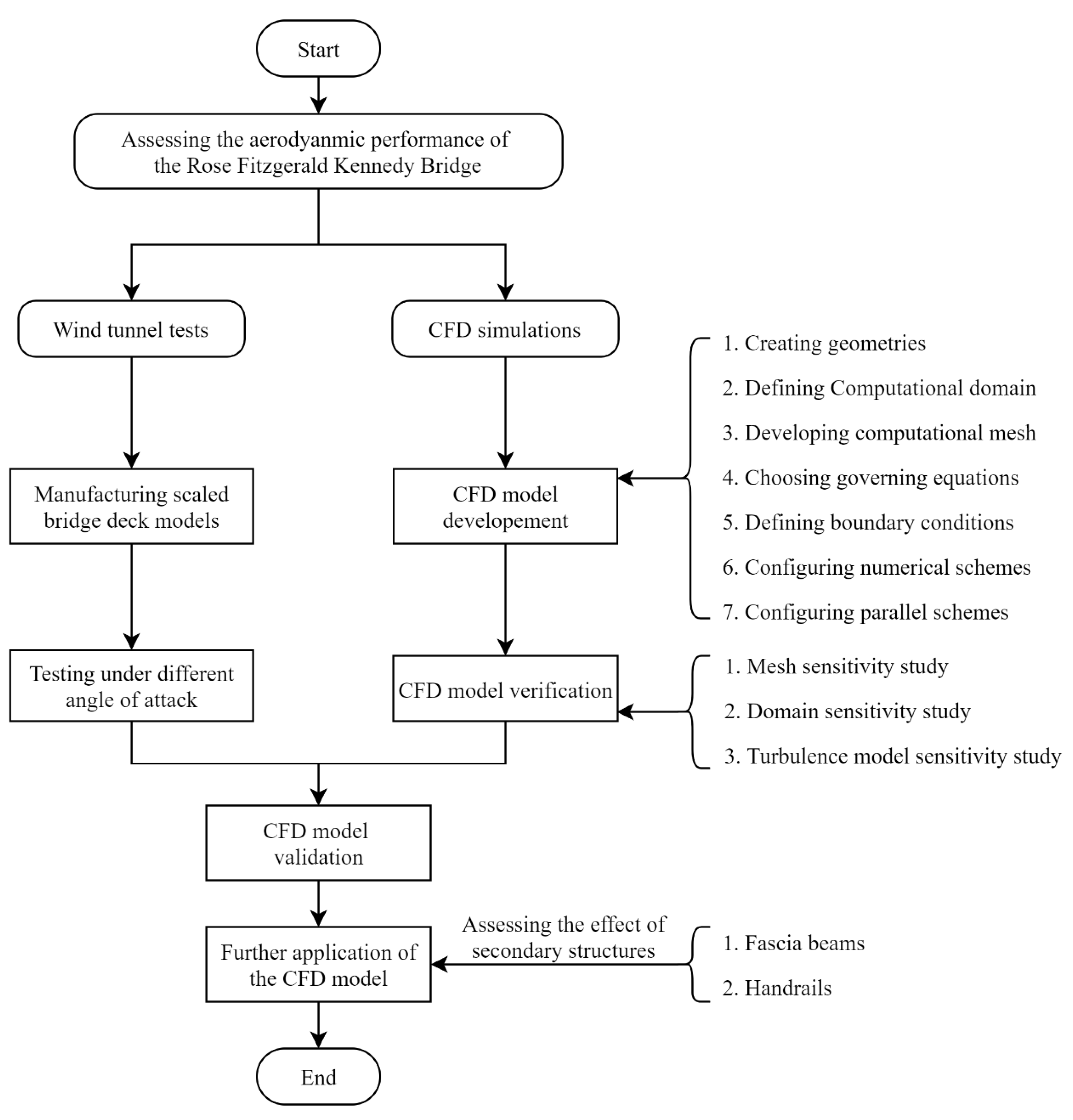
:1. Introduction
2. The Rose Kennedy Fitzgerald Bridge
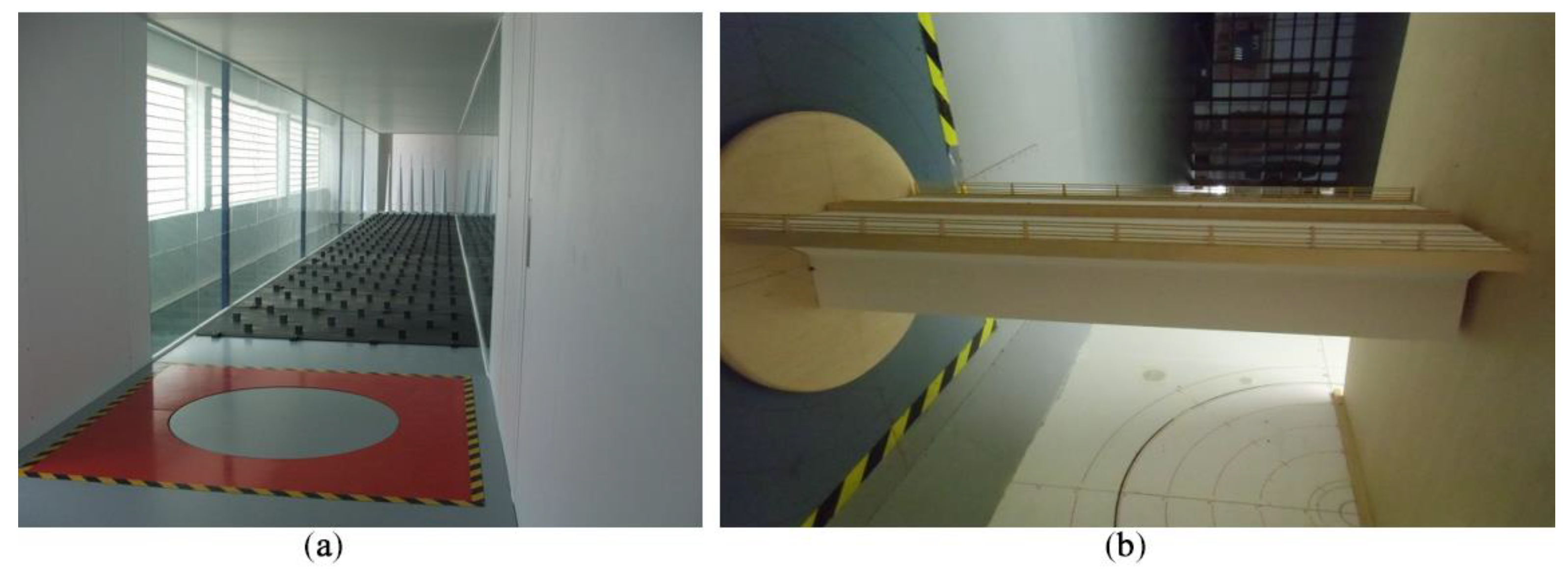
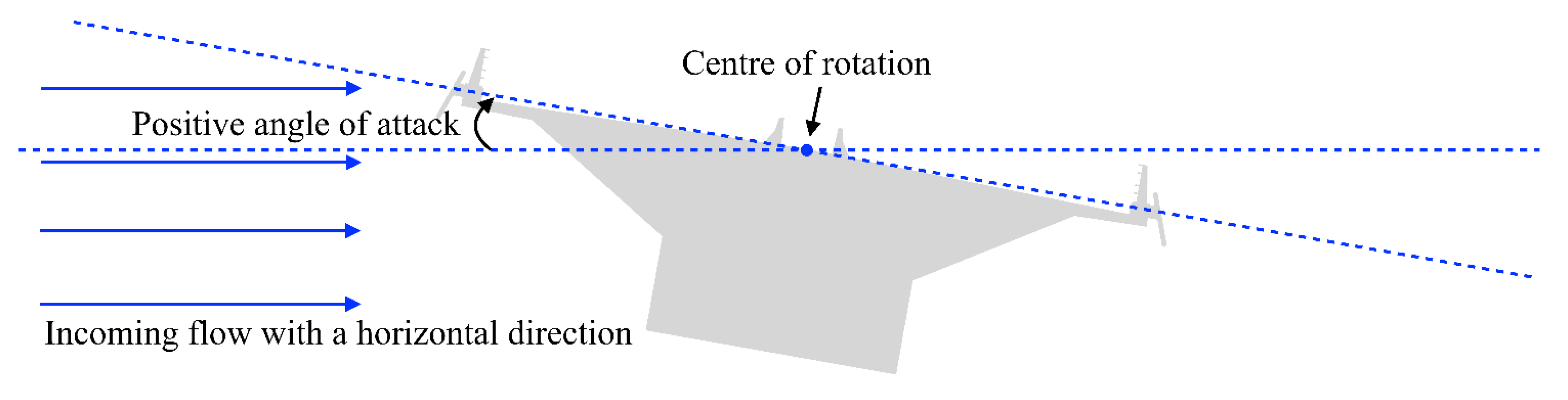
3. Description of the Wind Tunnel Tests
4. CFD Model
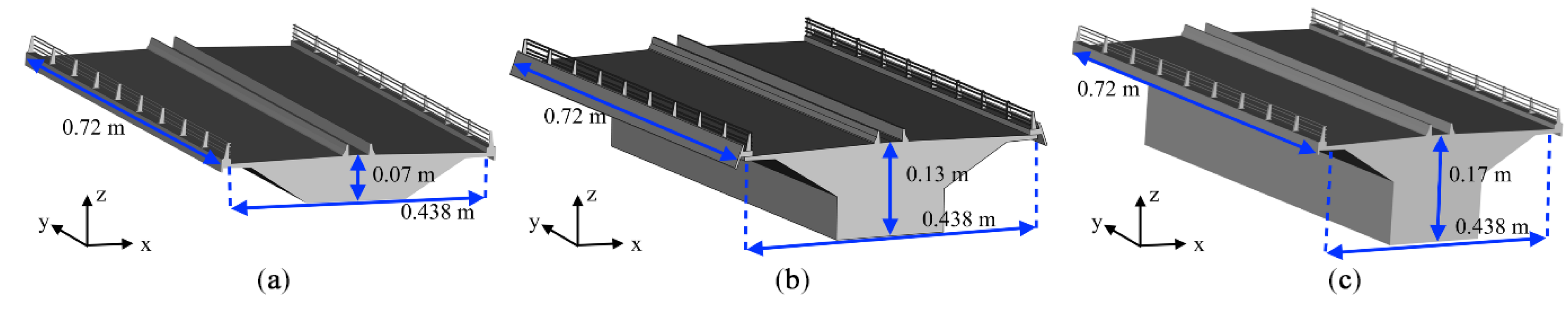
4.1. Geometry
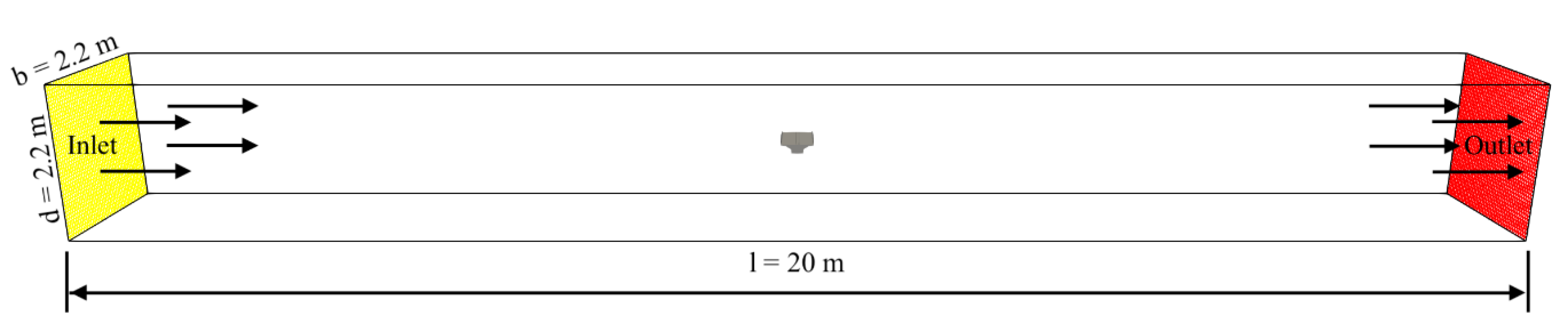
4.2. Computational Domain
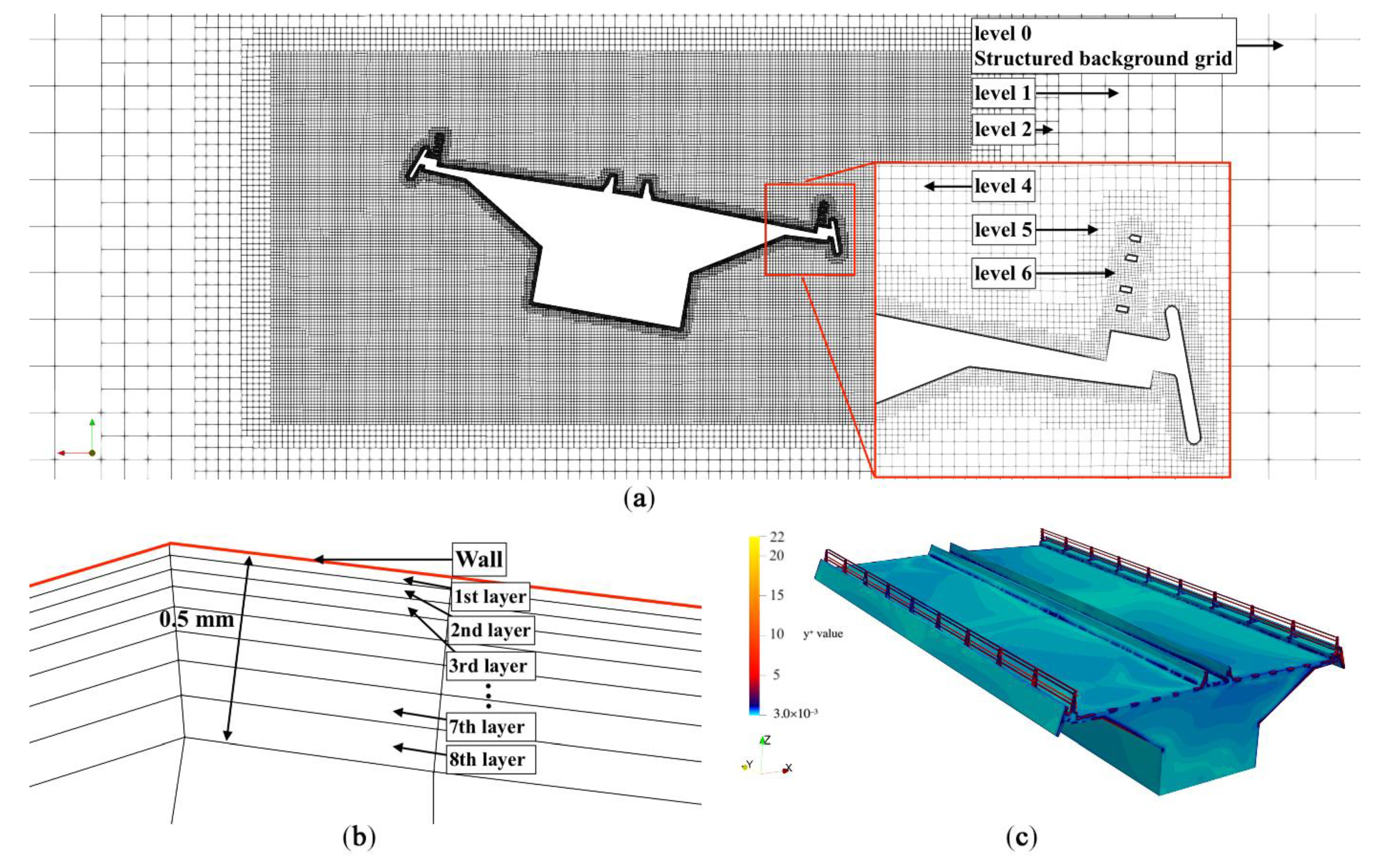
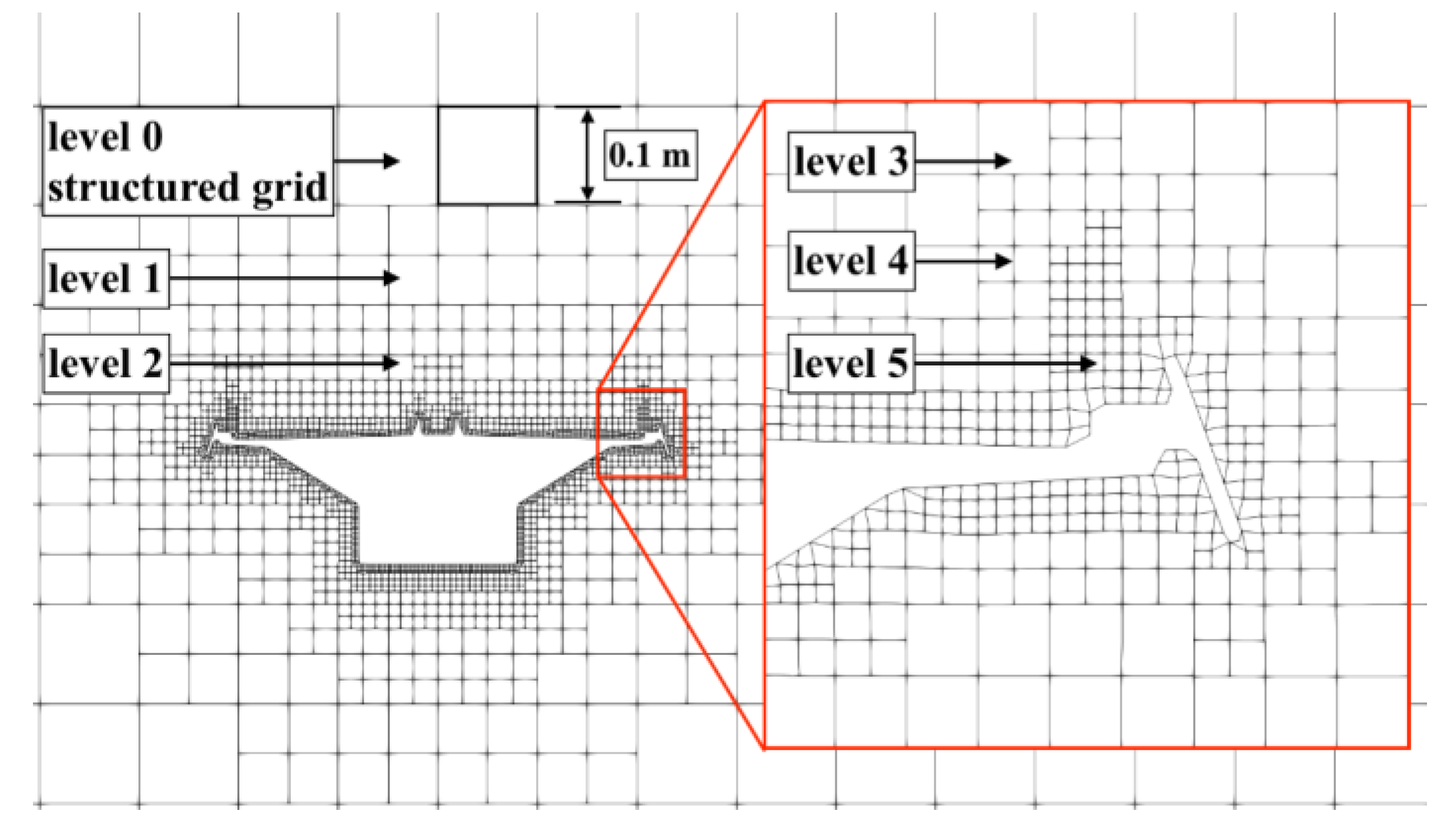
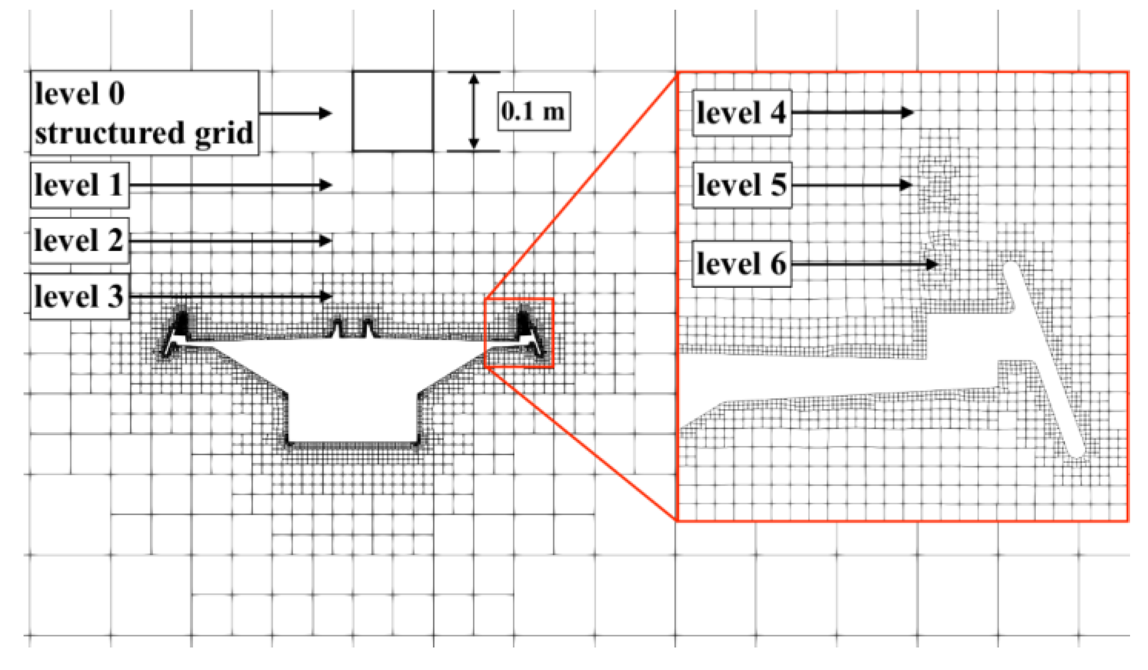
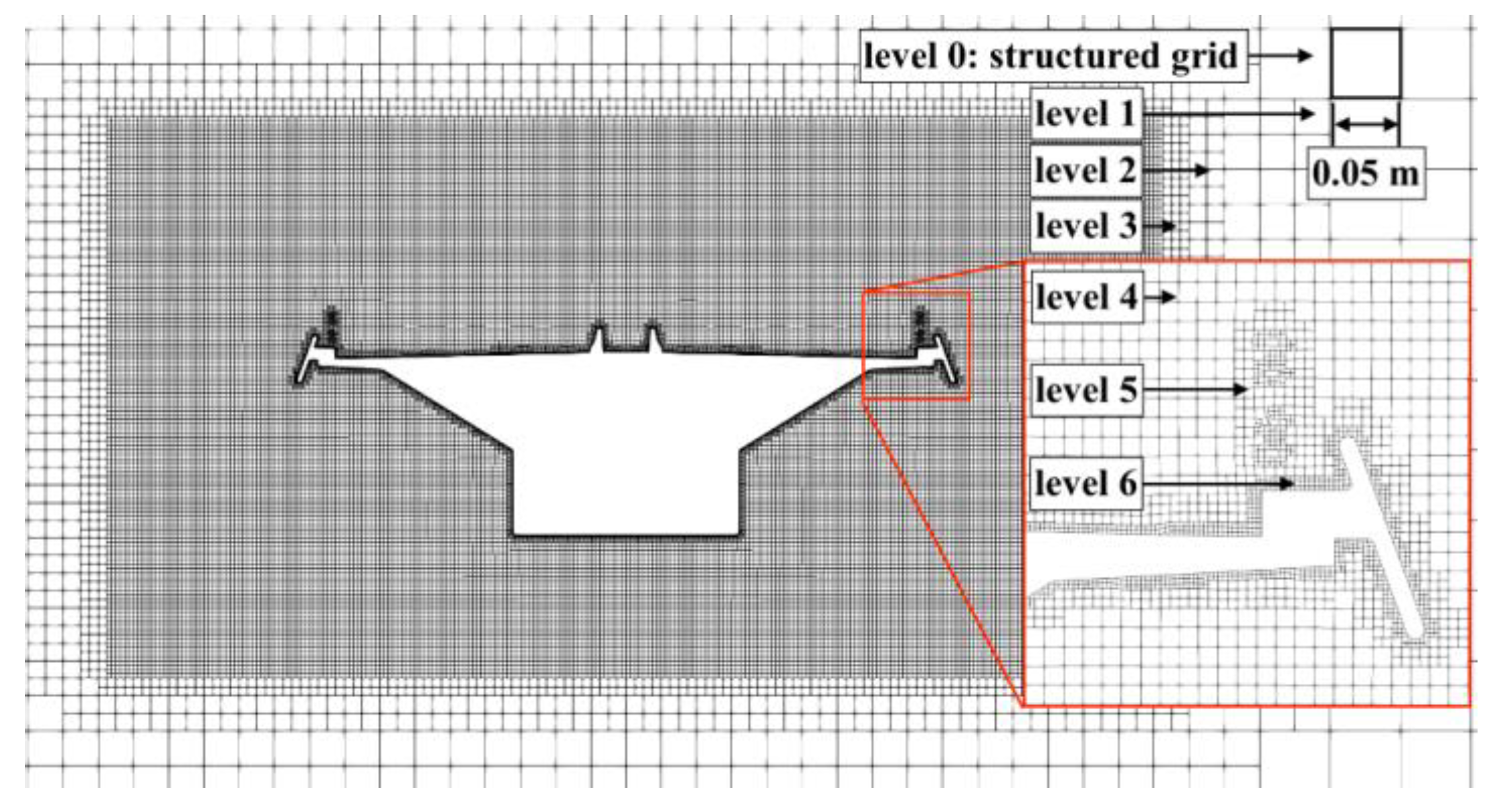
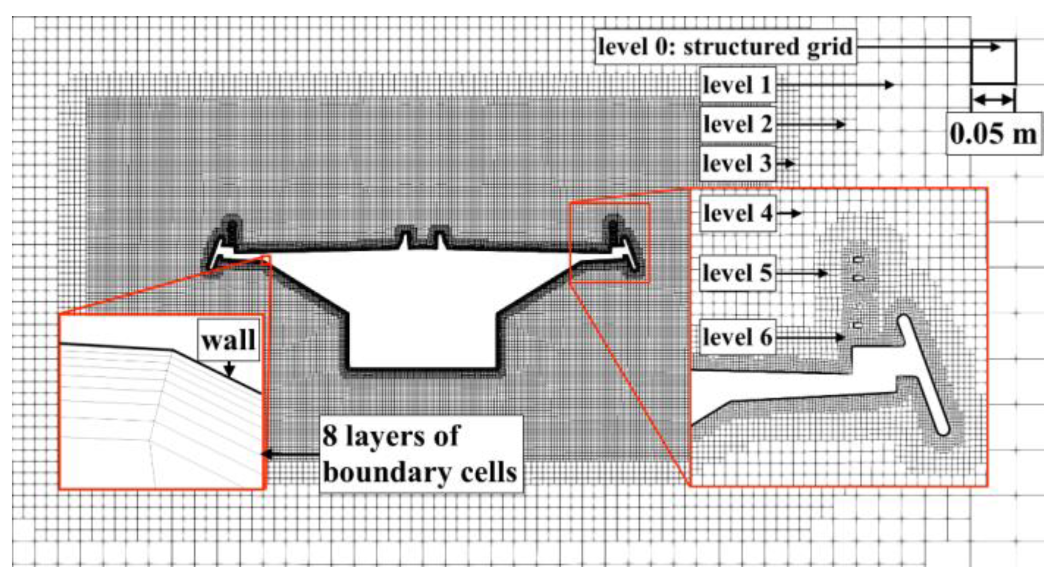
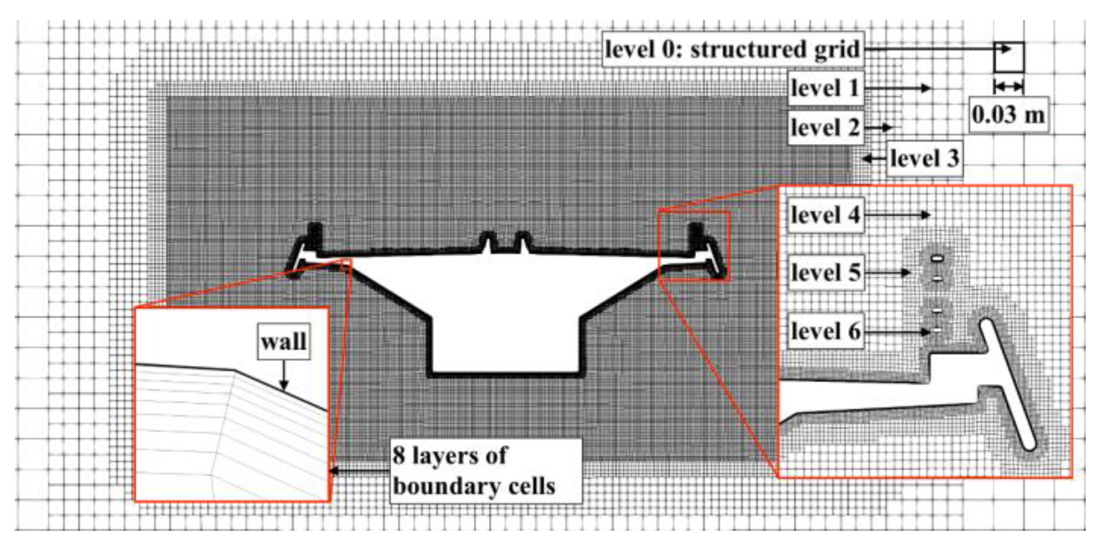
4.3. Computational Mesh
4.4. Governing Equations
4.5. Boundary Conditions
4.6. Numerical Configuration
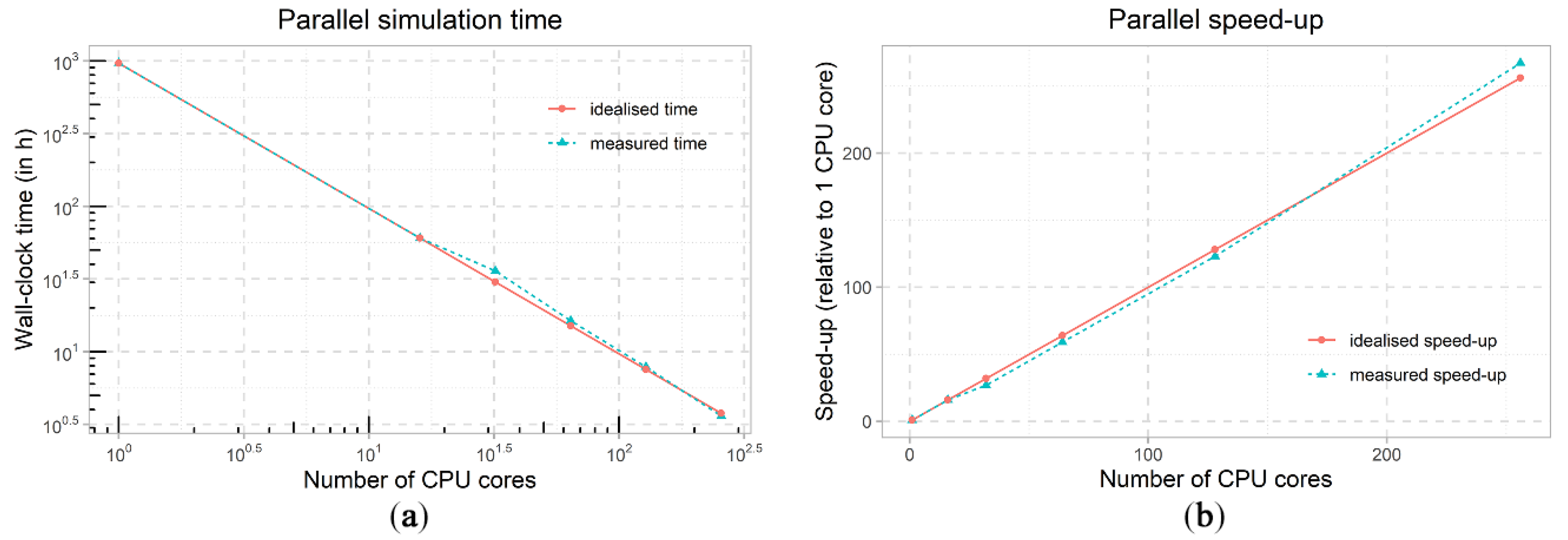
4.7. Parallel Configuration
5. Verification of the CFD Models
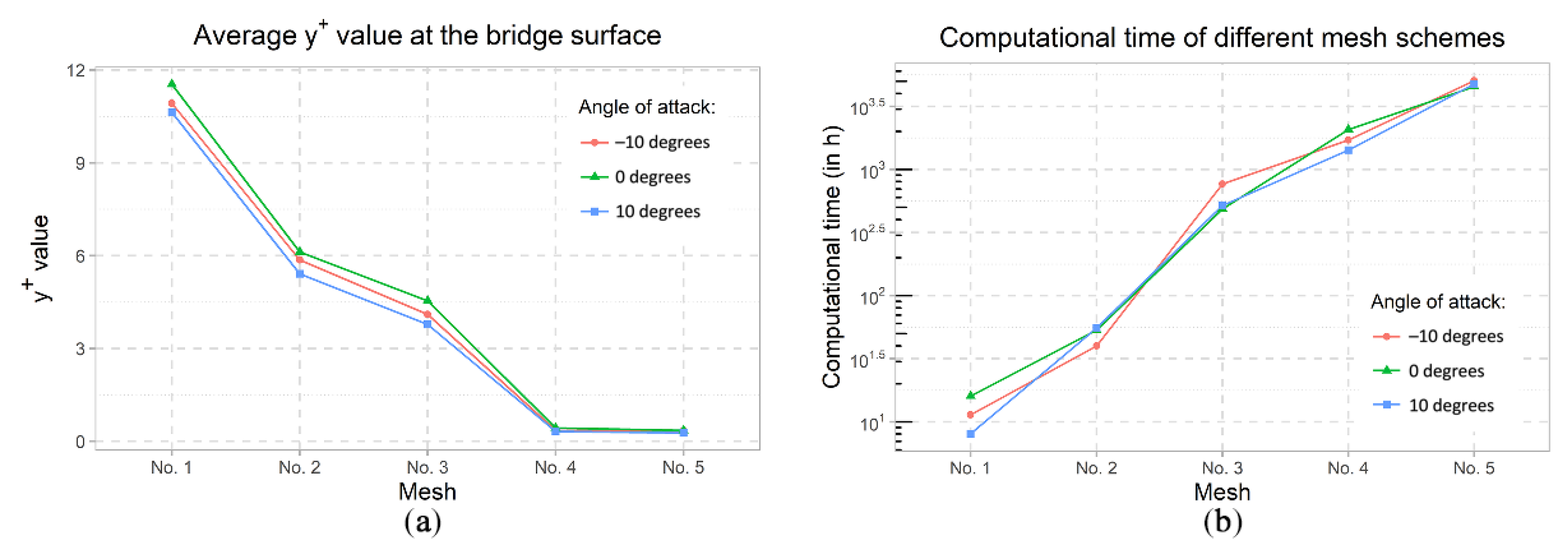
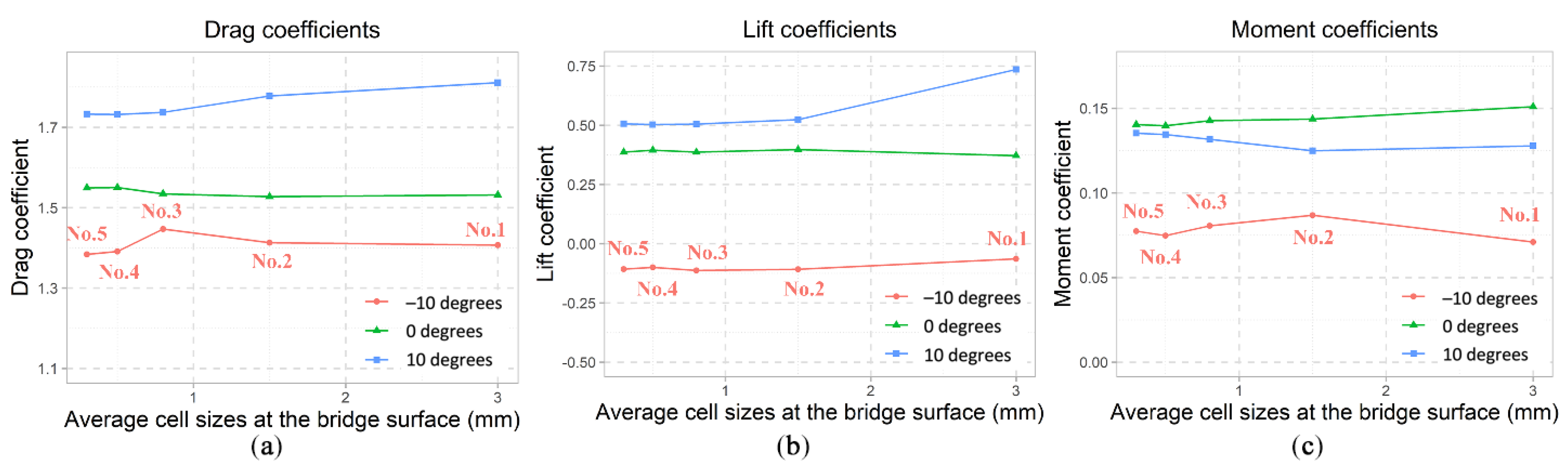
5.1. Mesh Sensitivity Analysis
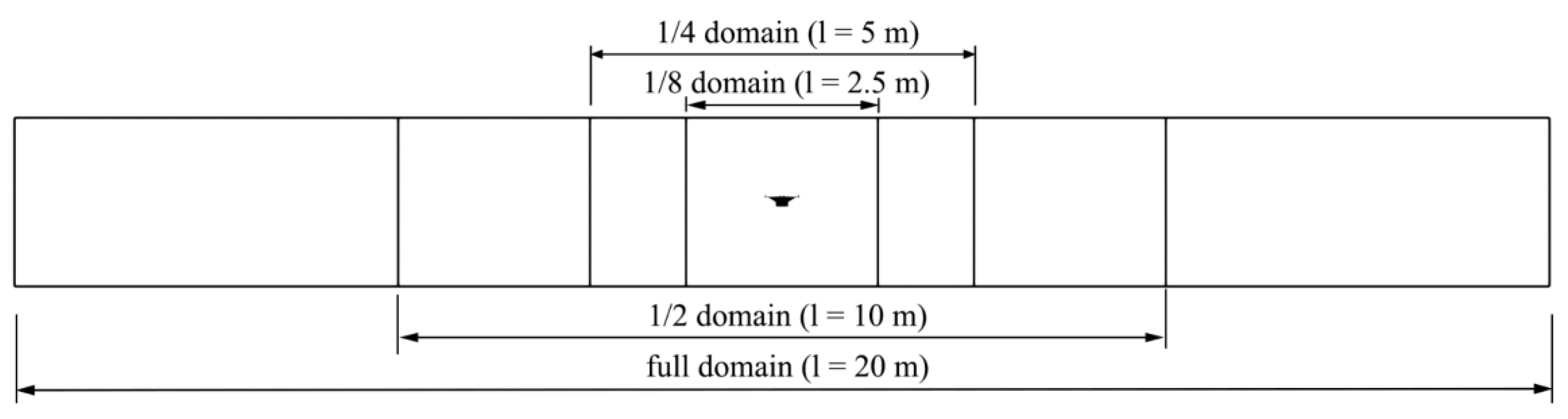
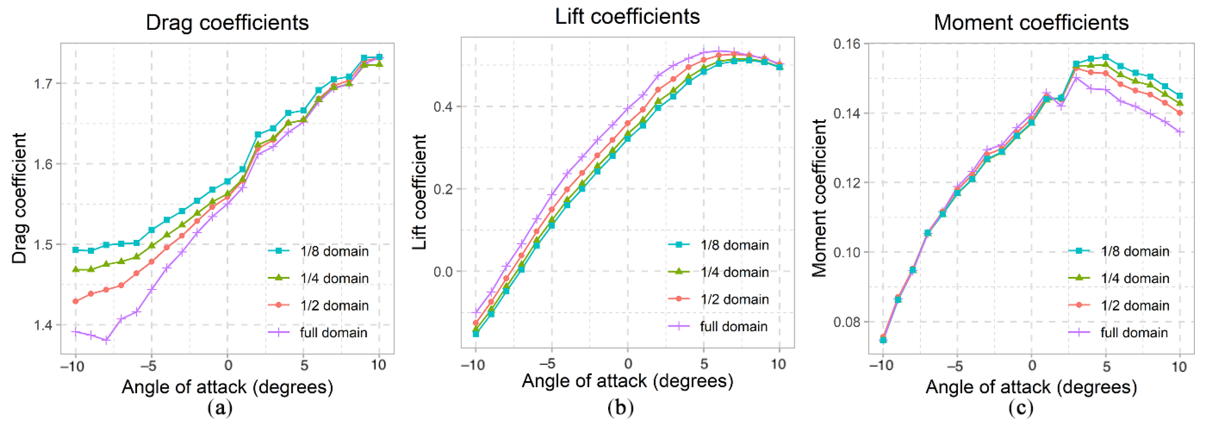
5.2. Domain Sensitivity Study
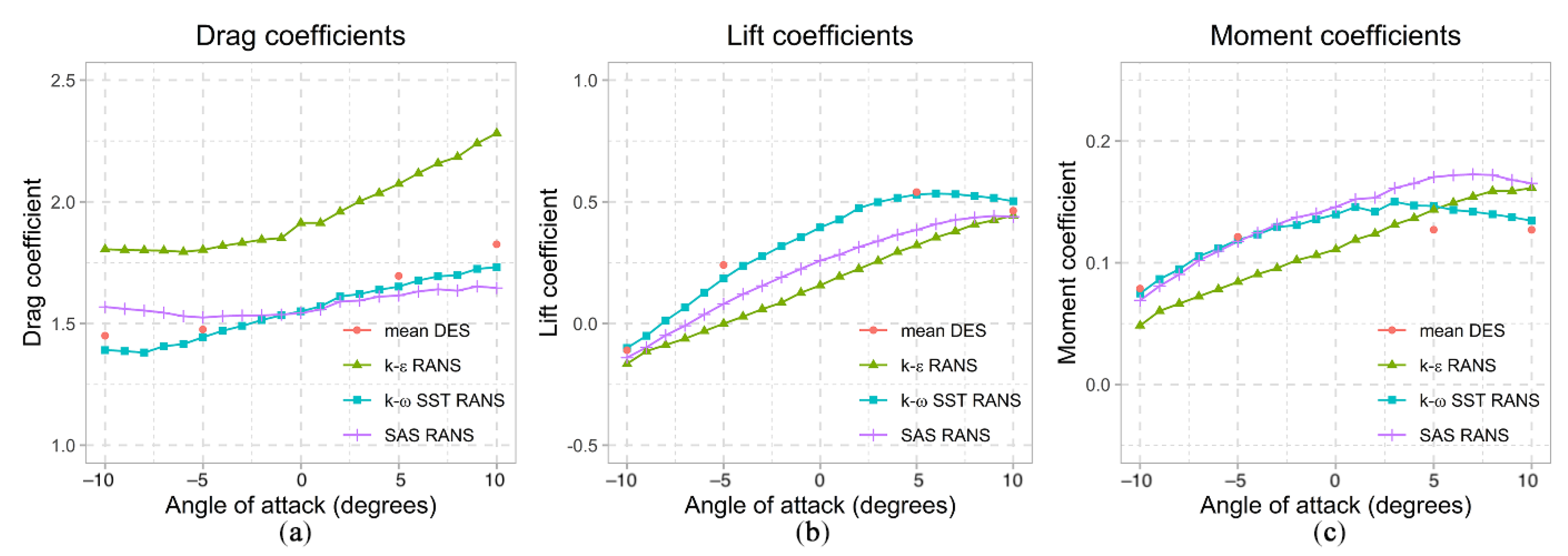
5.3. Sensitivity to Selection of Turbulence Model
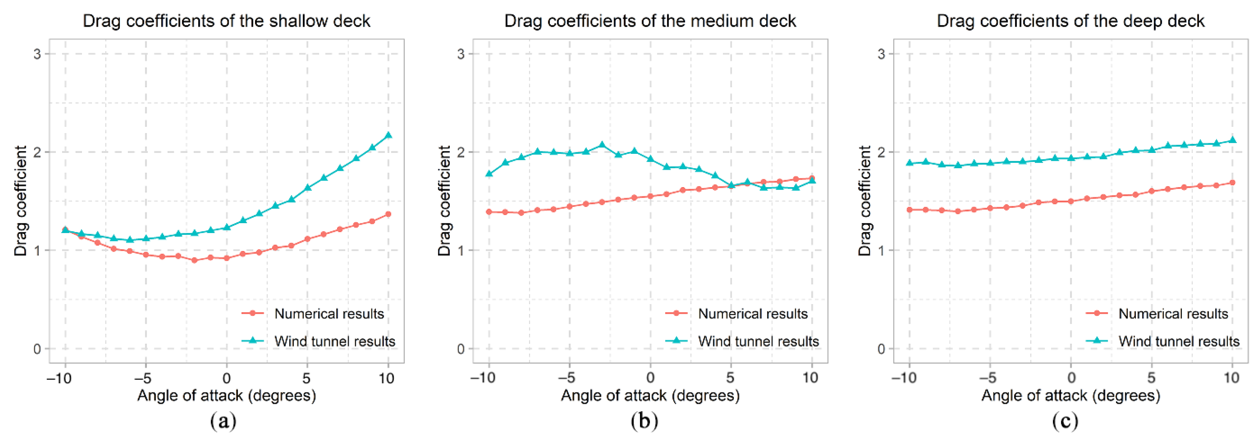
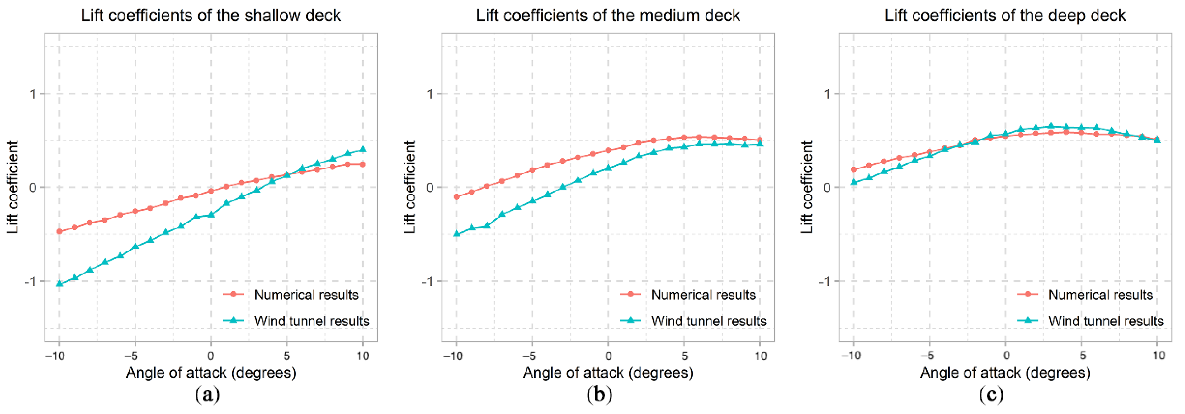
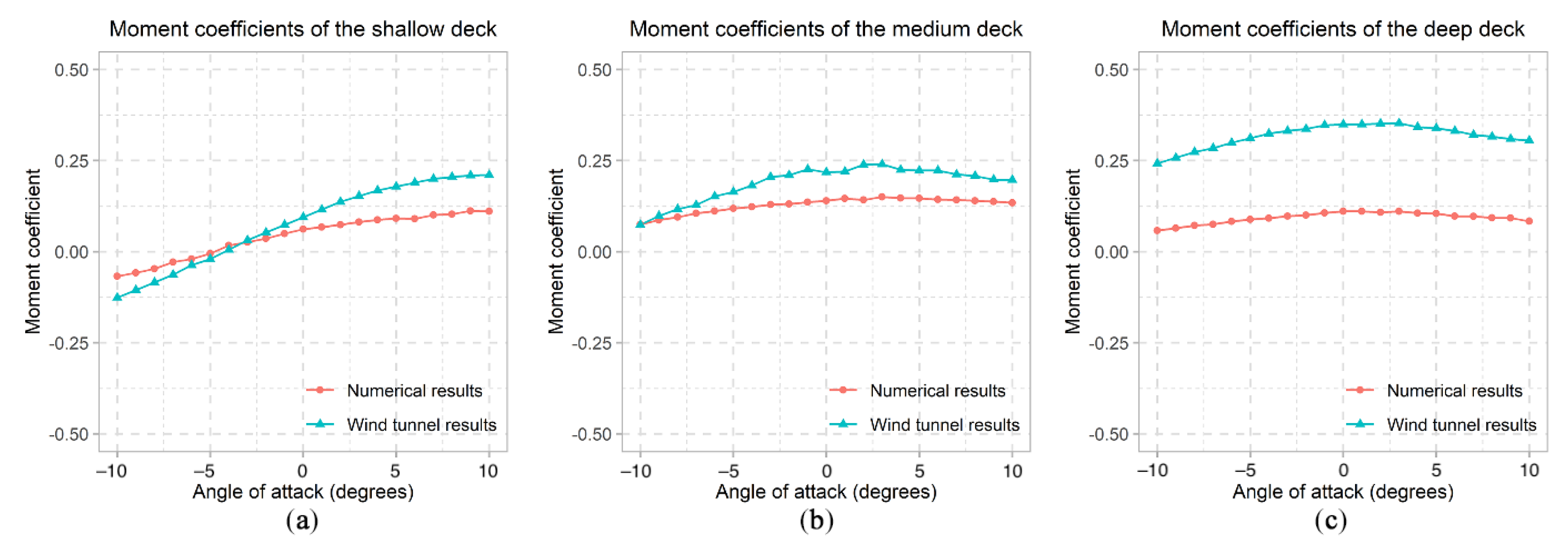
6. Validation of the CFD Models
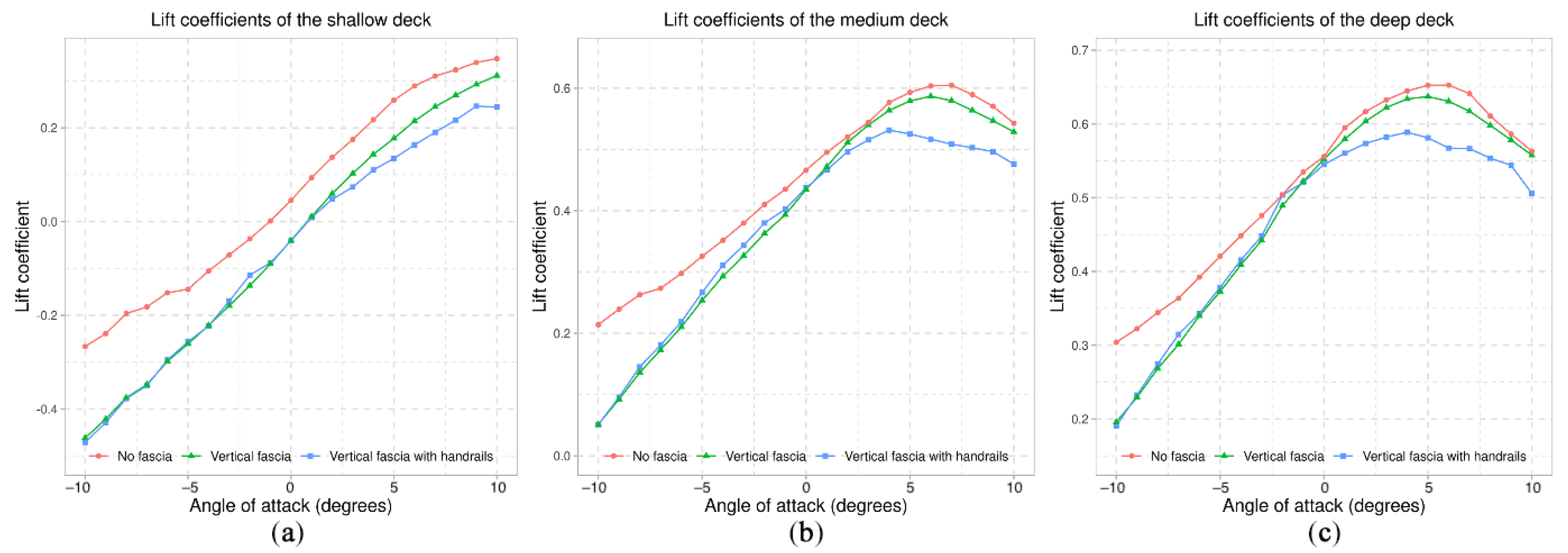
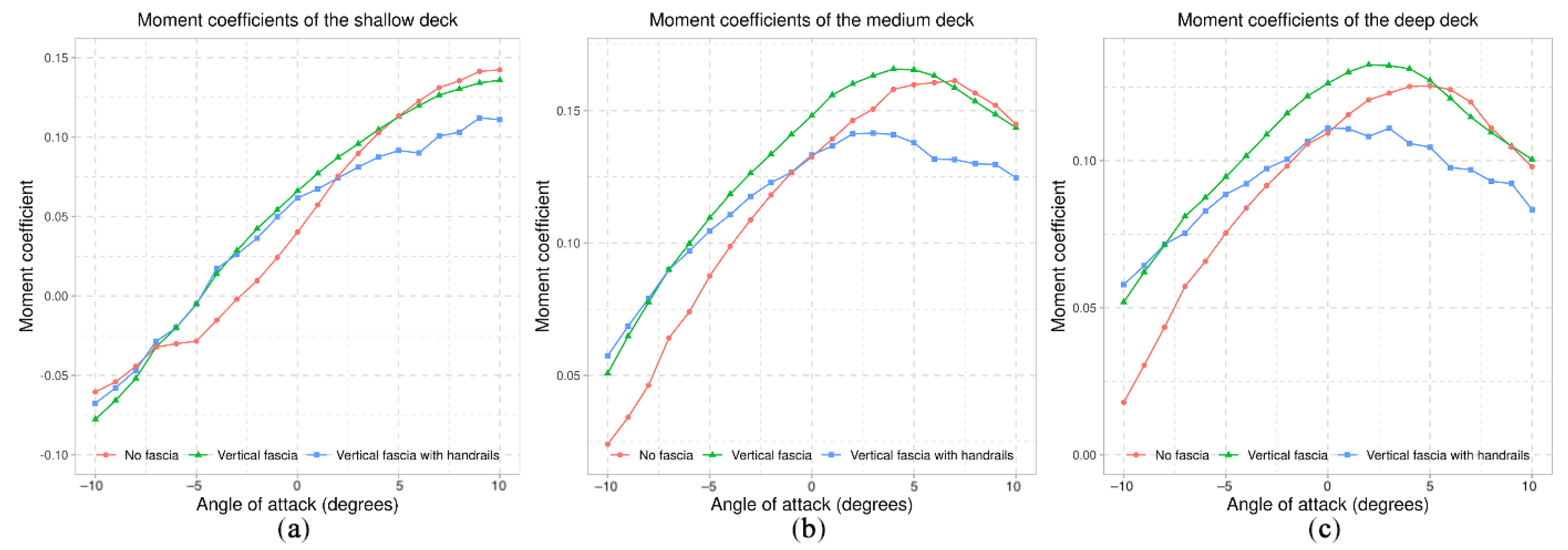
7. Assessing the Impact of Including Secondary Structures
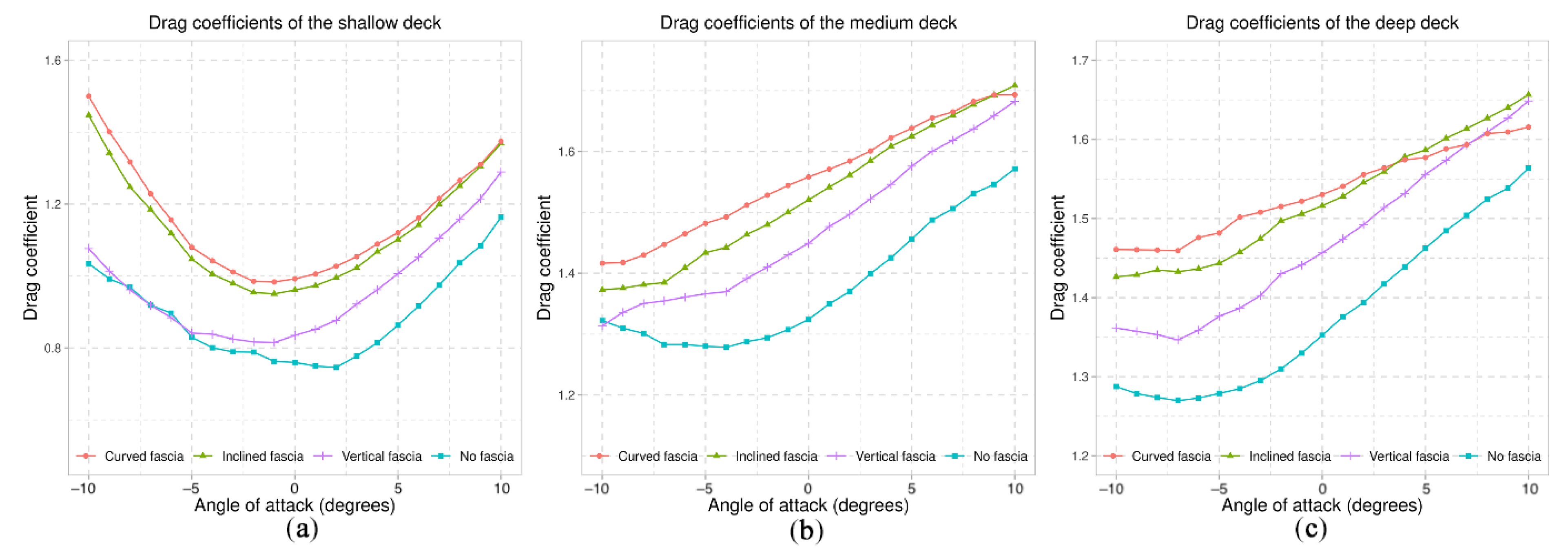
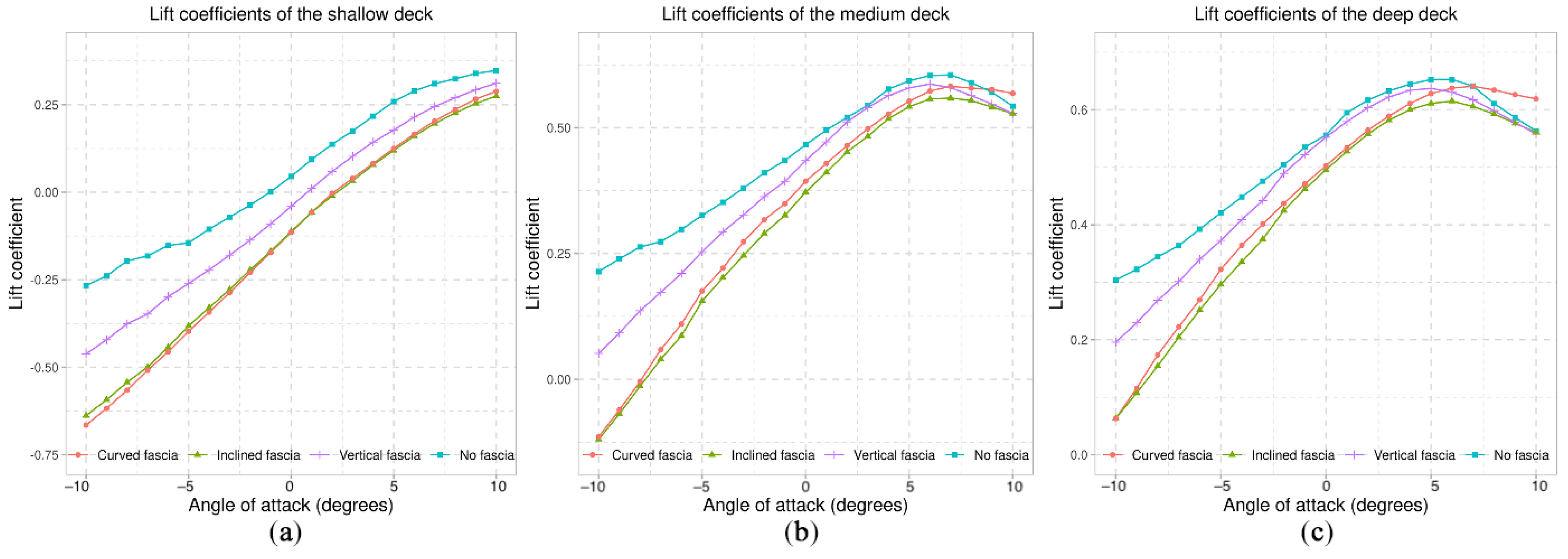
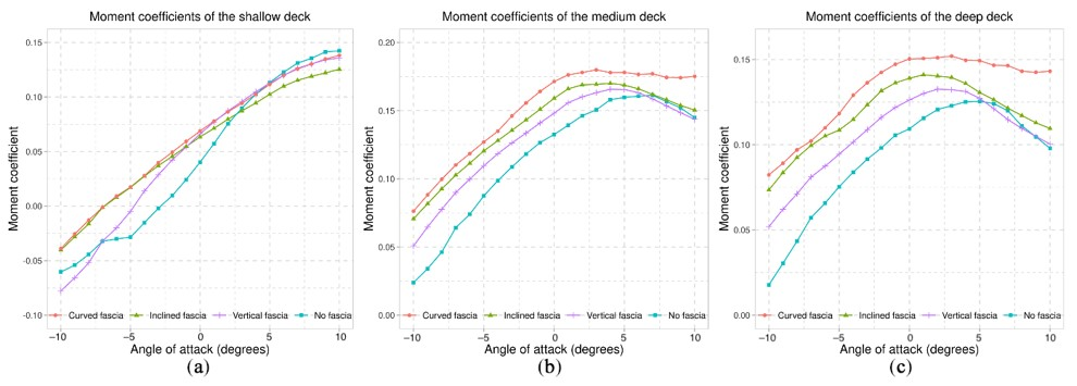
7.1. Fascia Beams
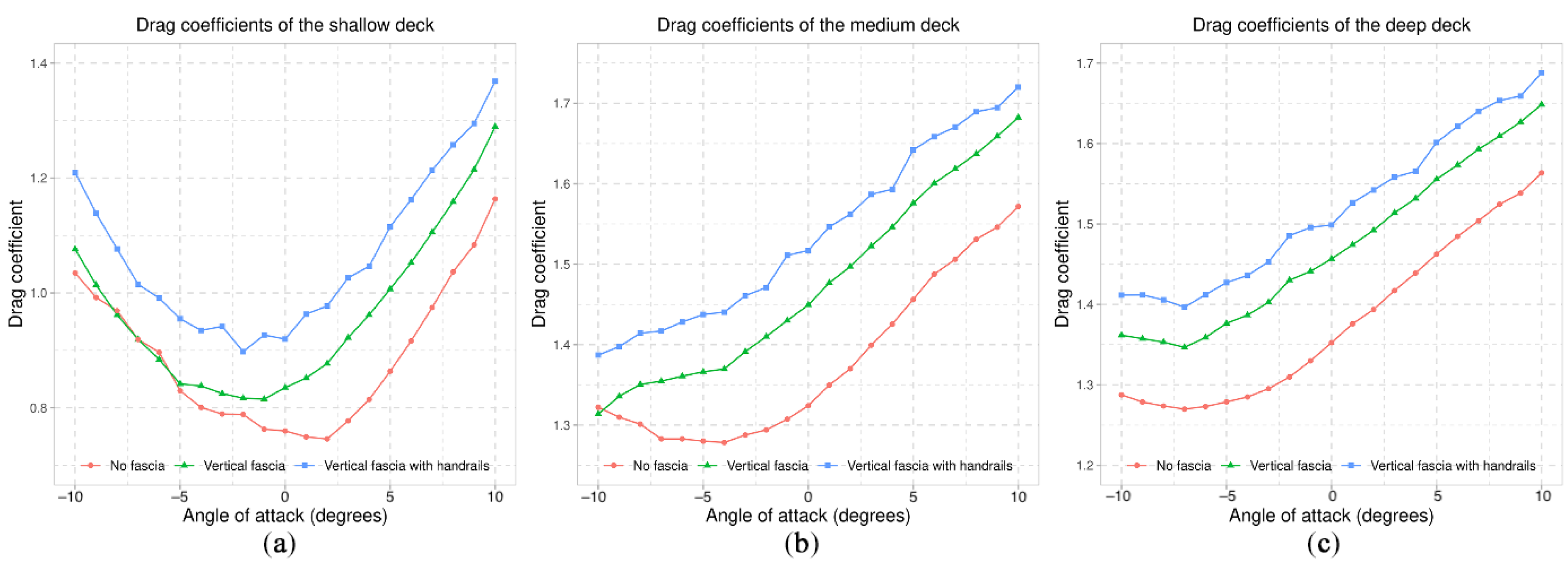
7.2. Handrails
8. Conclusions
Author Contributions
Funding
Data Availability Statement
Acknowledgments
Conflicts of Interest
References
- Kumarasena, S.; Jones, N.; Irwin, P.; Taylor, P. Wind-Induced Vibration of Stay Cables; Publication No. FHWA-RD-05-083; Technical Report; Federal Highway Administration: Springfield, VA, USA, 2007. [Google Scholar]
- Fujino, Y.; Yoshida, Y. Wind-induced vibration and control of Trans-Tokyo Bay crossing bridge. J. Struct. Eng. 2002, 128, 1012–1025. [Google Scholar] [CrossRef]
- Zhang, C. Humen Bridge remains closed after shaking. China Daily, 6 May 2020. [Google Scholar]
- Larsen, A.; Yeung, N.; Carter, M. Stonecutters Bridge, Hong Kong: Wind tunnel tests and studies. Proc. Inst. Civil Eng. Bridge Eng. 2012, 165, 91–104. [Google Scholar] [CrossRef]
- Ma, C.-m.; Duan, Q.-s.; Liao, H.-l. Experimental investigation on aerodynamic behavior of a long span cable-stayed bridge under construction. KSCE J. Civ. Eng. 2018, 22, 2492–2501. [Google Scholar] [CrossRef]
- Larsen, A.; Savage, M.; Lafrenière, A.; Hui, M.C.; Larsen, S.V. Investigation of vortex response of a twin box bridge section at high and low Reynolds numbers. J. Wind Eng. Ind. Aerodyn. 2008, 96, 934–944. [Google Scholar] [CrossRef]
- Marra, A.M.; Mannini, C.; Bartoli, G. Wind tunnel modeling for the vortex-induced vibrations of a yawed bridge tower. J. Bridge Eng. 2017, 22, 04017006. [Google Scholar] [CrossRef]
- Xin, D.; Zhang, H.; Ou, J. Experimental study on mitigating vortex-induced vibration of a bridge by using passive vortex generators. J. Wind Eng. Ind. Aerodyn. 2018, 175, 100–110. [Google Scholar] [CrossRef]
- Hu, C.; Zhao, L.; Ge, Y. Mechanism of suppression of vortex-induced vibrations of a streamlined closed-box girder using additional small-scale components. J. Wind Eng. Ind. Aerodyn. 2019, 189, 314–331. [Google Scholar] [CrossRef]
- Guntorojati, I. Flutter analysis of cable stayed bridge. Procedia Eng. 2017, 171, 1173–1177. [Google Scholar]
- Yang, Y.; Zhou, R.; Ge, Y.; Zhang, L. Flutter Characteristics of Thin Plate Sections for Aerodynamic Bridges. J. Bridge Eng. 2018, 23, 04017121. [Google Scholar] [CrossRef]
- Niu, H.; Zhu, J.; Chen, Z.; Zhang, W. Dynamic performance of a slender truss bridge subjected to extreme wind and traffic loads considering 18 flutter derivatives. J. Aerosp. Eng. 2019, 32, 04019082. [Google Scholar] [CrossRef]
- Mei, H.; Wang, Q.; Liao, H.; Fu, H. Improvement of Flutter Performance of a Streamlined Box Girder by Using an Upper Central Stabilizer. J. Bridge Eng. 2020, 25, 04020053. [Google Scholar] [CrossRef]
- Hikami, Y.; Shiraishi, N. Rain-wind induced vibrations of cables stayed bridges. J. Wind Eng. Ind. Aerodyn. 1988, 29, 409–418. [Google Scholar] [CrossRef]
- Jing, H.; Xia, Y.; Li, H.; Xu, Y.; Li, Y. Excitation mechanism of rain–wind induced cable vibration in a wind tunnel. J. Fluids Struct. 2017, 68, 32–47. [Google Scholar] [CrossRef]
- Cheng, P.; Li, W.-J.; Chen, W.-L.; Gao, D.-L.; Xu, Y.; Li, H. Computer vision-based recognition of rainwater rivulet morphology evolution during rain–wind-induced vibration of a 3D aeroelastic stay cable. J. Wind Eng. Ind. Aerodyn. 2018, 172, 367–378. [Google Scholar] [CrossRef]
- Gao, D.; Chen, W.; Eloy, C.; Li, H. Multi-mode responses, rivulet dynamics, flow structures and mechanism of rain-wind induced vibrations of a flexible cable. J. Fluids Struct. 2018, 82, 154–172. [Google Scholar] [CrossRef]
- Reddy, K.; Sharma, D.; Poddar, K. Effect of end plates on the surface pressure distribution of a given cambered airfoil: Experimental study. In New Trends in Fluid Mechanics Research; Springer: Berlin/Heidelberg, Germany, 2007; p. 286. [Google Scholar]
- Simiu, E.; Scanlan, R.H. Wind Effects on Structures: Fundamentals and Applications to Design; John Wiley: New York, NY, USA, 1996. [Google Scholar]
- Murakami, S.; Mochida, A. 3-D numerical simulation of airflow around a cubic model by means of the k-ϵ model. J. Wind Eng. Ind. Aerodyn. 1988, 31, 283–303. [Google Scholar] [CrossRef]
- Kuroda, S. Numerical simulation of flow around a box girder of a long span suspension bridge. J. Wind Eng. Ind. Aerodyn. 1997, 67, 239–252. [Google Scholar] [CrossRef]
- Selvam, R.P.; Tarini, M.J.; Larsen, A. Computer modelling of flow around bridges using LES and FEM. J. Wind Eng. Ind. Aerodyn. 1998, 77, 643–651. [Google Scholar] [CrossRef]
- Anina, Š.; Ruediger, H.; Stanko, B. Numerical simulations and experimental validations of force coefficients and flutter derivatives of a bridge deck. J. Wind Eng. Ind. Aerodyn. 2015, 144, 172–182. [Google Scholar] [CrossRef]
- Xu, F.; Zhang, Z. Free vibration numerical simulation technique for extracting flutter derivatives of bridge decks. J. Wind Eng. Ind. Aerodyn. 2017, 170, 226–237. [Google Scholar] [CrossRef]
- Helgedagsrud, T.A.; Bazilevs, Y.; Mathisen, K.M.; Øiseth, O.A. Computational and experimental investigation of free vibration and flutter of bridge decks. Comput. Mech. 2019, 63, 121–136. [Google Scholar] [CrossRef]
- Sarwar, M.W.; Ishihara, T. Numerical study on suppression of vortex-induced vibrations of box girder bridge section by aerodynamic countermeasures. J. Wind Eng. Ind. Aerodyn. 2010, 98, 701–711. [Google Scholar] [CrossRef]
- Zhang, H.; Xin, D.; Ou, J. Wake control using spanwise-varying vortex generators on bridge decks: A computational study. J. Wind Eng. Ind. Aerodyn. 2019, 184, 185–197. [Google Scholar] [CrossRef]
- Zhang, T.; Sun, Y.; Li, M.; Yang, X. Experimental and numerical studies on the vortex-induced vibration of two-box edge girder for cable-stayed bridges. J. Wind Eng. Ind. Aerodyn. 2020, 206, 104336. [Google Scholar] [CrossRef]
- Chen, X.; Qiu, F.; Tang, H.; Li, Y.; Xu, X. Effects of Secondary Elements on Vortex-Induced Vibration of a Streamlined Box Girder. KSCE J. Civ. Eng. 2021, 25, 173–184. [Google Scholar] [CrossRef]
- Li, H.; Chen, W.-L.; Xu, F.; Li, F.-C.; Ou, J.-P. A numerical and experimental hybrid approach for the investigation of aerodynamic forces on stay cables suffering from rain-wind induced vibration. J. Fluids Struct. 2010, 26, 1195–1215. [Google Scholar] [CrossRef]
- Xie, P.; Zhou, C.Y. Numerical investigation on effects of rivulet and cable oscillation of a stayed cable in rain-wind-induced vibration. J. Mech. Sci. Technol. 2013, 27, 685–701. [Google Scholar] [CrossRef]
- Bi, J.; Guan, J.; Wang, J.; Lu, P.; Qiao, H.; Wu, J. 3d numerical analysis on wind and rain induced oscillations of water film on cable surface. J. Wind Eng. Ind. Aerodyn. 2018, 176, 273–289. [Google Scholar] [CrossRef]
- Jing, H.; He, X.; Wang, Z. Numerical modeling of the wind load of a two-dimensional cable model in rain–wind-induced vibration. J. Fluids Struct. 2018, 82, 121–133. [Google Scholar] [CrossRef]
- Zhang, Y.; Cardiff, P.; Keenahan, J. Wind-Induced Phenomena in Long-Span Cable-Supported Bridges: A Comparative Review of Wind Tunnel Tests and Computational Fluid Dynamics Modelling. Appl. Sci. 2021, 11, 1642. [Google Scholar] [CrossRef]
- Liu, L.; Zhang, L.; Wu, B.; Chen, B. Effect of Accessory Attachment on Static Coefficients in a Steel Box Girder for Long-Span Suspension Bridges. J. Eng. Sci. Technol. Rev. 2017, 10, 68–83. [Google Scholar] [CrossRef]
- Li, Y.-L.; Chen, X.-Y.; Yu, C.-J.; Togbenou, K.; Wang, B.; Zhu, L.-D. Effects of wind fairing angle on aerodynamic characteristics and dynamic responses of a streamlined trapezoidal box girder. J. Wind Eng. Ind. Aerodyn. 2018, 177, 69–78. [Google Scholar] [CrossRef]
- Kusano, I.; Jakobsen, J.B.; Snæbjörnsson, J.T. CFD simulations of a suspension bridge deck for different deck shapes with railings and vortex mitigating devices. IOP Conf. Ser. Mater. Sci. Eng. 2019, 700, 012003. [Google Scholar] [CrossRef]
- Jeong, W.; Liu, S.; Bogunovic Jakobsen, J.; Ong, M.C. Unsteady RANS simulations of flow around a twin-box bridge girder cross section. Energies 2019, 12, 2670. [Google Scholar] [CrossRef] [Green Version]
- He, X.; Zhou, L.; Chen, Z.; Jing, H.; Zou, Y.; Wu, T. Effect of wind barriers on the flow field and aerodynamic forces of a train–bridge system. Proc. Inst. Mech. Eng. Part F J. Rail Rapid Transit 2019, 233, 283–297. [Google Scholar] [CrossRef]
- Bowe, M.; Murphy, J.; Shinkwin, J. The Rose Fitzgerald Kennedy Bridge; PROF-ENG: Velká Hraštice, Czech Republic, 2020. [Google Scholar]
- ASCE. Wind Tunnel Testing for Buildings and Other Structures ASCE/SEI 49-12; American Society of Civil Engineers: Washington, DC, USA, 2012. [Google Scholar]
- Gutiérrez, M.O.; Longhi, S.F.; Ortega, O.G. Wind Loads and Wind Condition on a Section of the New Ross Bypass Bridge (Ireland); Universidad Politécnica de Madrid: Madrid, Spain, 2017. [Google Scholar]
- Eurocode, C. 1: Actions on Structures–Part 1.4: General Actions–Wind Actions; The European Standard EN: Brussels, Belgium, 2005. [Google Scholar]
- Menter, F.R.; Kuntz, M.; Langtry, R. Ten years of industrial experience with the SST turbulence model. Turbul. Heat Mass Transf. 2003, 4, 625–632. [Google Scholar]
- Nguyen, V.-M.; Phan, T.-H.; Phan, H.-N.; Nguyen, D.-A.; Ha, M.-N.; Nguyen, D.-T. Three-Dimensional Study on Aerodynamic Drag Coefficients of Cable-Stayed Bridge Pylons by Finite Element Method. In Structural Health Monitoring and Engineering Structures; Springer: Singapore, 2021; pp. 489–498. [Google Scholar]
- Patankar, S.V.; Spalding, D.B. A calculation procedure for heat, mass and momentum transfer in three-dimensional parabolic flows. In Numerical Prediction of Flow, Heat Transfer, Turbulence and Combustion; Elsevier: Amsterdam, The Netherlands, 1983; pp. 54–73. [Google Scholar]
- Jasak, H. Error Analysis and Estimation for the Finite Volume Method with Applications to Fluid Flows. Ph.D. Thesis, University of London, London, UK, 1996. [Google Scholar]
- Barrett, R.; Berry, M.; Chan, T.F.; Demmel, J.; Donato, J.; Dongarra, J.; Eijkhout, V.; Pozo, R.; Romine, C.; Van der Vorst, H. Templates for the Solution of Linear Systems: Building Blocks for Iterative Methods; SIAM: Philadelphia, PA, USA, 1994. [Google Scholar]
- Van der Vorst, H.A. Bi-CGSTAB: A fast and smoothly converging variant of Bi-CG for the solution of nonsymmetric linear systems. SIAM J. Sci. Stat. Comput. 1992, 13, 631–644. [Google Scholar] [CrossRef]
- Issa, R.I. Solution of the implicitly discretised fluid flow equations by operator-splitting. J. Comput. Phys. 1986, 62, 40–65. [Google Scholar] [CrossRef]
- Chevalier, C.; Pellegrini, F. PT-Scotch: A tool for efficient parallel graph ordering. Parallel Comput. 2008, 34, 318–331. [Google Scholar] [CrossRef] [Green Version]
- Venkatesh, T.; Sarasamma, V.; Rajalakshmy, S.; Sahu, K.C.; Govindarajan, R. Super-linear speed-up of a parallel multigrid Navier–Stokes solver on Flosolver. Curr. Sci. 2005, 88, 589–593. [Google Scholar]
- Cardiff, P.; Karač, A.; Ivanković, A. A large strain finite volume method for orthotropic bodies with general material orientations. Comput. Methods Appl. Mech. Eng. 2014, 268, 318–335. [Google Scholar] [CrossRef]
- Launder, B.E.; Spalding, D.B. The numerical computation of turbulent flows. In Numerical Prediction of Flow, Heat Transfer, Turbulence and Combustion; Elsevier: Amsterdam, The Netherlands, 1983; pp. 96–116. [Google Scholar]
- Spalart, P.; Allmaras, S. A One-Equation Turbulence Model for Aerodynamic Flows. In Proceedings of the 30th Aerospace Sciences Meeting and Exhibit, Reno, NV, USA, 6–9 January 1992; p. 439. [Google Scholar]
- Tominaga, Y.; Mochida, A.; Murakami, S.; Sawaki, S. Comparison of various revised k–ε models and LES applied to flow around a high-rise building model with 1:1:2 shape placed within the surface boundary layer. J. Wind Eng. Ind. Aerodyn. 2008, 96, 389–411. [Google Scholar] [CrossRef]
- Sun, D.; Owen, J.; Wright, N. Application of the k–ω turbulence model for a wind-induced vibration study of 2D bluff bodies. J. Wind Eng. Ind. Aerodyn. 2009, 97, 77–87. [Google Scholar] [CrossRef]
- Han, Y.; Chen, H.; Cai, C.; Xu, G.; Shen, L.; Hu, P. Numerical analysis on the difference of drag force coefficients of bridge deck sections between the global force and pressure distribution methods. J. Wind Eng. Ind. Aerodyn. 2016, 159, 65–79. [Google Scholar] [CrossRef]
- Holmes, J.D. Wind Loading of Structures; CRC Press: Boca Raton, FL, USA, 2007. [Google Scholar]
- Takeda, K.; Kato, M. Wind tunnel blockage effects on drag coefficient and wind-induced vibration. J. Wind Eng. Ind. Aerodyn. 1992, 42, 897–908. [Google Scholar] [CrossRef]
- Kubo, Y.; Miyazaki, M.; Kato, K. Effects of end plates and blockage of structural members on drag forces. J. Wind Eng. Ind. Aerodyn. 1989, 32, 329–342. [Google Scholar] [CrossRef]
- Jiang, B.; Zhou, Z.; Yan, K.; Hu, C. Effect of Web Inclination of Streamlined Flat Box Deck on Aerostatic Performance of a Bridge. J. Bridge Eng. 2021, 26, 04020126. [Google Scholar] [CrossRef]


| Boundary Region | Parameter | Type | Value | Unit | Surface-Normal Gradient |
|---|---|---|---|---|---|
| Inlet | U | Dirichlet | 5.9 | m/s | - |
| p | Neumann | - | m2/s2 | 0 | |
| k | Dirichlet | 1.17 | m2/s2 | - | |
| ω | Dirichlet | 2.9 | s−1 | - | |
| outlet | U | Neumann | - | m/s | 0 |
| p | Dirichlet | 0 | m2/s2 | - | |
| k | Neumann | - | m2/s2 | 0 | |
| ω | Neumann | - | s−1 | 0 | |
| wall | U | no-slip | 0 | m/s | - |
| p | Neumann | - | m2/s2 | 0 | |
| k | Adaptive wall function | - | m2/s2 | - | |
| ω | Adaptive wall function | - | s−1 | - |
| Parameter | Linear Solver | Solving Tolerance |
|---|---|---|
| p | Preconditioned conjugate gradient [48] | 1 × 10⁻¹¹ |
| U, k, ω, ε, | Preconditioned bi-conjugate gradient [49] | 1 × 10⁻¹¹ |
| Number of CPU Cores | Wall-Clock Time (In h) | Speed-Up | Cells Per CPU Core |
|---|---|---|---|
| 1 | 965.28 (estimated) | - | 33,189,094 |
| 16 | 60.33 | 16 | 1,937,500 |
| 32 | 35.88 | 26.903 | 968,750 |
| 64 | 16.31 | 59.172 | 484,375 |
| 128 | 7.84 | 123.023 | 242,188 |
| 256 | 3.61 | 267.175 | 121,094 |
| Configurations | Cell Count of Mesh No.1 | Cell Count of Mesh No.2 | Cell Count of Mesh No.3 | Cell Count of Mesh No.4 | Cell Count of Mesh No.5 |
|---|---|---|---|---|---|
| −10° | 452,138 | 1,962,324 | 14,607,636 | 33,242,170 | 85,922,392 |
| 0° | 454,144 | 1,973,227 | 14,575,020 | 33,189,094 | 86,008,513 |
| 10° | 448,144 | 1,972,355 | 14,608,860 | 33,227,289 | 86,441,092 |
| Boundary Region | k, (In the k-ε Model) | ε, (In the k-ε Model) | (In the SAS Model) |
|---|---|---|---|
| inlet | Dirichlet (1.17 m2/s2) | Dirichlet (0.56 m2/s3) | Dirichlet (0.74 m2/s) |
| outlet | Neumann with zero surface-normal gradient | Neumann with zero surface-normal gradient | Neumann with zero surface-normal gradient |
| wall | adaptive wall function | adaptive wall function | adaptive wall function |
Publisher’s Note: MDPI stays neutral with regard to jurisdictional claims in published maps and institutional affiliations. |
© 2021 by the authors. Licensee MDPI, Basel, Switzerland. This article is an open access article distributed under the terms and conditions of the Creative Commons Attribution (CC BY) license (https://creativecommons.org/licenses/by/4.0/).
Share and Cite
Zhang, Y.; Cardiff, P.; Cahill, F.; Keenahan, J. Assessing the Capability of Computational Fluid Dynamics Models in Replicating Wind Tunnel Test Results for the Rose Fitzgerald Kennedy Bridge. CivilEng 2021, 2, 1065-1090. https://0-doi-org.brum.beds.ac.uk/10.3390/civileng2040057
Zhang Y, Cardiff P, Cahill F, Keenahan J. Assessing the Capability of Computational Fluid Dynamics Models in Replicating Wind Tunnel Test Results for the Rose Fitzgerald Kennedy Bridge. CivilEng. 2021; 2(4):1065-1090. https://0-doi-org.brum.beds.ac.uk/10.3390/civileng2040057
Chicago/Turabian StyleZhang, Yuxiang, Philip Cardiff, Fergal Cahill, and Jennifer Keenahan. 2021. "Assessing the Capability of Computational Fluid Dynamics Models in Replicating Wind Tunnel Test Results for the Rose Fitzgerald Kennedy Bridge" CivilEng 2, no. 4: 1065-1090. https://0-doi-org.brum.beds.ac.uk/10.3390/civileng2040057