
Use of Fibre-Optic Sensors for Pipe Condition and Hydraulics Measurements: A Review


1
Department of Mechanical Engineering, University of Sheffield, Sheffield S1 3JD, UK
2
Department of Civil and Structural Engineering, University of Sheffield, Sheffield S1 3JD, UK
*
Author to whom correspondence should be addressed.
CivilEng 2022, 3(1), 85-113; https://0-doi-org.brum.beds.ac.uk/10.3390/civileng3010006
Submission received: 11 November 2021
/
Revised: 21 January 2022
/
Accepted: 24 January 2022
/
Published: 27 January 2022
(This article belongs to the Special Issue Early Career Stars in Civil Engineering)
Abstract
:The combined length of the sewerage and clean water pipe infrastructure in the UK is estimated to be about 800,000 km. It is prone to failure due to its age and the inadequacies of the current pipe inspection methods. Fibre-optic cable sensing is an attractive way to continuously monitor this infrastructure to detect critical changes. This paper reviews the existing fibre-optic sensor (FOS) technologies to suggest that these technologies have better sensing potential than traditional inspection and performance monitoring methods. This review also discusses the requirements for retrofitting an existing pipeline with an FOS. It also demonstrates that there is a need for further research into methods applicable to non-pressurised pipelines, as there is very little existing literature that focuses on partially filled pipes and pipes with gravity fed flows.
1. Introduction
Over recent years, the benefits of accurate monitoring of buried pipe infrastructure have become more and more apparent to asset owners. It is estimated that the total length of the buried utilities network in the UK is about 1.5 million km [1], which includes around 400,000 km of sewerage network and the clean water pipe network of a similar length [2]. These assets are ageing and are prone to deterioration and unexpected failure. Little is known about their condition, as the existing methods of pipe monitoring mostly rely on infrequent single-location inspections, and they are expensive and slow. The lack of knowledge about pipe condition results in unanticipated failures [3]; for example, deteriorating clean water pipes result in leakages, by which the amount of lost water is estimated to be 3000 million litres of water per day (or 20% of the total water supply) in England alone, which has a significant impact on the total water demand [4]. Failing pipes also lead to street works and the disruptions associated with them. It has been estimated that around 4.25 million holes are dug in the streets in the UK every year, and the cost of the utility trenching is over £1.5 billion per year [1]. These statistics make it clear that possessing knowledge about the state of buried pipe infrastructure has money- and labour-saving benefits because it can lead to a much more proactive economic maintenance and rehabilitation programme that would result in a large reduction in unexpected failures.
The United Stated Environmental Protection Agency (US EPA) defines pipe condition assessment as, “The collection of data and information through direct inspection, observation and investigation and in-direct monitoring and reporting, and the analysis of the data and information to make a determination of the structural, operational and performance status of capital infrastructure assets” [5]. Current methods of pipe inspection are varied and have been extensively reviewed elsewhere [6,7,8]. These methods can be divided into direct and indirect, where direct sensing methods involved visual inspection, non-destructive testing and pipe sampling, whereas indirect methods rely on testing water and measuring such quantities as flow rate and soil resistivity to determine the degree of pipe deterioration [6]. A summary of some common methods is as follows.
1.1. Direct Methods
1.1.1. Visual Inspection
This category includes closed-circuit television (CCTV) inspection and laser scanning methods administered from inside the pipe. A CCTV inspection unit consists of a camera and a lighting device installed on a carrier that can be moved through stormwater or sewage pipes at speeds of between 15 and 30 cm/s. The recorded data are examined manually and post-survey, which slows the process down. A laser scanning device acquires information on the inner profile of a pipe for subsequent analysis to determine such quantities as diameter, perimeter and cross-sectional area. The accuracy of this method depends on the pipe roughness and colour, but some devices exhibit both high scanning speed and high resolution [9]. It is unusual to run CCTV and laser scans in water-filled pipes.
1.1.2. Acoustic and Ultrasonic Methods
There is a wide variety of techniques and devices that employ these methods [8], so only some will be reviewed here. The impact echo method is a common test for determining the thickness and geometry of a pipe. It relies on hitting a test surface with an impact hammer and recording its response with an accelerometer positioned in the vicinity of the impact. It can be used for most pipe materials and sizes but requires access to the pipe wall, either externally or internally. Several commercially-available devices have been widely used for leak detection. These include LeakFinderRT [10] that detects leaks by using two accelerometers or hydrophones attached to two contact points on a pipe and determining a time lag between two leak-generated signals. This methods has an advantage of working well for small leaks and high background noise. SmartBall technology [11] makes use of a passive sensor that travels with water flow and detects the presence, location and size of leaks. Sahara device [12] utilises a hydrophone to locate leaks in water mains. SewerBatt instrument [13] is positioned at an entrance to a pipe through a manhole to detect wall damage, lateral connections and blockages by analysing the acoustic wave reflected from these artefacts. Ultrasonic methods include guided wave ultrasound, where the signal propagates along the pipe and signature of the reflected signal determines the location and size of a defect, ultrasound that utilises a point transducer to estimate the thickness of a pipe wall to detect corrosion and the phased array technology [14] that employs sound beams with different shape and direction, enabling the interpretation of complex defects such as metal loss and wall cracks.
1.1.3. Electromagnetic Methods
The majority of electromagnetic methods employ eddy currents. The remote field eddy current (RFEC) system uses an exciting coil driven by low-frequency alternating current and one or more detector coils that are placed inside a pipe. An electromagnetic field between these coils propagates freely through the pipe, and any changes in its magnitude or phase can be attributed to discontinuities in the pipe. Broadband electromagnetic (BEM) technique is similar to RFEC but uses a broadband signal rather than single-frequency. Pulsed eddy current (PEC) testing enables the estimation of a steel pipe wall thickness by measuring the strength of the magnetic field at a distance from the pipe surface and relating it to the pipe thickness. Non-eddy current methods include the ground penetrating radar (GPR) which relies on transmitting electromagnetic signal into the ground and relating the reflected signal to underground events, such as voids caused by leaks or abnormal depth of pipe caused by changes in signal propagation velocity as it travels through water-saturated soil. The magnetic flux leakage (MFL) method creates magnetic fields in the wall of a ferrous pipe using large magnets, where the anomalies will result in changing the magnetic flux distribution. It can only be used on a pipe exterior and in clean, unlined pipes.
1.1.4. Radiographic Methods
These methods use gamma (for ferrous and concrete pipes) and X-ray (for plastic pipes) signals to map voids or material irregularities in a pipe by sending the signal through the material onto a photographic plate or a digital camera. The X-ray method has a limitation that pipes of a diameter of 381 mm or over have to be emptied before the inspection.
1.1.5. Thermography Methods
Thermographic testing uses an external source of heat to heat up a pipe to be inspected and an infrared (IR) camera to monitor the cooling of the pipe. By examining its cooling characteristics, it is possible to determine whether the pipe has any damage. The above methods are relatively expensive and used mainly to inspect critical pipe infrastructure in petrochemical and nuclear industries.
1.2. Indirect Methods
A comprehensive summary of indirect pipe inspection methods is given in a report by Marlow et al. [15]. Some of these methods are reviewed below.
1.2.1. Soil Characterisation
This method explores soil parameters that can be related to deterioration of buried pipes. There parameters include soil resistivity (lower resistivity is linked to higher corrosion), pH (values below 4 or above 8 are linked to corrosion of ferrous pipes), and sulfate content (its variation can impact cement leaching leading to pipe wall thinning [15]).
1.2.2. Linear Polarisation Resistance (LPR) of Soil
Corrosion in pipes often happens due to being subjected to saturated soil that acts as an electrolyte. One of the methods of deducing the rate of corrosion of a pipe is to measure an electric current that is induced as a result of an applied weak potential difference between two electrodes. This current will be directly proportional to the current that causes corrosion, and subsequently, to the rate of corrosion of the pipe.
1.2.3. Pipe to Soil Potential Survey
This method can be applied to determine gaps in protective coating of a ferrous pipe or its rate of corrosion. For the former application, the direct current voltage gradient (DCVG) method can be used, where a direct current is applied to the pipe and two electrodes are moved along its surface, looking for anomalies in measured voltage. For the latter, one electrode is used to determine the pipe-to-soil potential around the pipe.
1.3. The Case for a New Method
However, these methods in general are slow, require direct contact with the pipe surface and involve human intervention.
The outlined issues with existing pipe surveillance methods signify that there is the need for novel monitoring techniques that can be applied to a variety of pipelines and can detect defects with high accuracy and over a prolonged period of time. One of the potential methods that meets these criteria is a sensor based on fibre-optic cable technology. Optical fibres have been extensively used for communications and remote or distributed sensing since the 1970s, when losses in them were reduced to 20 dB/km [16]. The advantages of sensors based on optical fibres are numerous. Above all, fibre-optic sensors do not require electrical power and combine low optical transmission losses and little signal deterioration, which enables them to transmit massive volumes of information fast and over long distances. The geometry of the sensor makes it compact, flexible and light-weight. Fibre-optic sensors are impervious to electric and magnetic disturbances, and can withstand harsh environments, such as high temperatures and corrosion. At the same time, they are highly sensitive to physical disturbances such as strain, temperature and pressure, among others. Finally, using a fibre-optic sensor eliminates the need for additional fibres, as the same fibre can be used for sensing and transmitting information. This is especially beneficial when using distributed sensing as one fibre can act as multiple sensors while only requiring one cable to connect it to a data acquisition system.
Fibre-optic sensors have been extensively used in a variety of civil engineering applications related to structural health monitoring (SHM) [17,18,19], including some hydraulic applications, mainly in the oil and gas industry [20]. They are able to detect small leaks with 1–2 m accuracy within 10 s of a leak occurring [21]. Fibre-optic sensors are also highly durable, withstanding 30 years in service with minimum maintenance. However, as it will be shown later in this review, the majority of all previous applications are implemented in pressurised pipes. This reveals a gap in research on using fibre-optic sensors in partially-filled pipes, such as sewer or drainage pipes, despite the significant length of the non-pressurised pipeline network. This paper aims to review the existing literature on using fibre-optic sensing techniques in hydraulic and hydrodynamic scenarios, and create a summary of different sensing techniques and their applications. This will then be used to inform research on the use of fibre-optic sensors for partially-filled pipes. It is also important to note that the notion of temperature sensing with fibre-optic sensors is an established research topic and will not be reviewed in this paper, where the main focus will be acoustic and strain sensing, i.e., response of fibre-optic sensor to external pressure or strain stimuli.
This paper is structured as follows. Section 2 covers principles of fibre-optic sensing, including the physics of fibre optics and an overview of different types of fibre-optic sensors. Section 3 reviews the existing research in using fibre-optic sensors for hydraulic applications. Section 4 offers a summary of the presented information, and compares and contrasts different sensing methods. Section 5 presents the conclusions of this review.
2. Principles of Fibre-Optic Sensing
Optical fibres came into widespread use in the second half of the 20th century. It became possible due to the invention of the laser [22], the understanding that optical fibres make suitable waveguides for light propagation [23] and reduction of transmission loss in optical fibres to 20 dB/km [24]. These advances in technology enabled the development of fibre-optic sensors starting with a fotonic sensor in 1967 [25] that accurately measured the distance between a bundle of optical fibres and a given surface. Other areas of application followed, including acoustic and strain sensing with optical fibres [26], fibre-optic hydrophones [27] and strain gauges [28]. In order to proceed with an in-depth review of the applications of fibre-optic sensors, it would be of benefit to review the physical principles of fibre-optic sensing.
2.1. Fundamentals of Fibre Optics
The light propagation in an optical fibre relies on well understood optical phenomena. The principle of refraction states that light is deflected from its original path when passing obliquely between two media with different densities (or refractive indices). This can be expressed mathematically with the following expression, also known as Snell’s law:
where is the refractive index of a medium in which light is travelling initially, is the refractive index of a medium into which the light is refracted, is the angle between an incident ray and the normal line, and is the angle between a refracted ray and the normal line. At smaller incident angles, when light travels from a more dense to a less dense medium, both reflection and refraction occur at the same time. However, as the value of the incident angle increases and reaches a certain value , the light ray does not refract into a lower-index medium but instead it propagates along the interface between the two media. With the increasing values of the incident angle , light is fully reflected within the higher-index medium. This phenomenon is called total internal reflection (TIR) and it is used to enable long-range light propagation in an optical fibre, as shown in Figure 1. A light ray is incident on the interface between air and glass as it enters the core of the optical fibre, resulting in its refraction on entry. As it propagates through the core, it fully reflects off its wall, with no light refracting into a cladding, which has a lower refractive index ( in this example). The difference between the refractive indices of core and cladding is called the numerical aperture (NA), and it determines the light-acceptance capability of an optical fibre. A larger NA enables the optical fibre to accept incident light rays at higher incidence angles.
The two basic types of optical fibres are single mode and multimode, which is determined by the geometry of a fibre. In a single mode fibre, the diameter of the core is much smaller than that in a multimode fibre, resulting in less dispersion associated with multi-path propagation of light. Optical fibres can be step-index (both single mode and multimode) or graded-index (only multimode). In a step-index optical fibre, the refractive index that is constant throughout the core undergoes a step change at the interface to a different value of the refractive index in the cladding. In a graded-index optical fibre, the refractive index of the core gradually decreases with increasing distance from the fibre axis. Graded-index optical fibres are mostly used to enable the transmission of high quantities of information, and are not of great use in fibre-optic sensors [29].
The amount of light propagating in an optical fibre is dependent on the losses, or attenuation in the fibre. The attenuation is typically measured in terms of losses in dB per unit length, or dB/km. There are numerous causes for attenuation and these include impurities or imperfections within the fibre core that can cause scattering or absorption, micro- or macrobending, and fibre end loss due to end face defects. However, some of these losses act as mechanisms underlying fibre-optic sensing and will be covered in more detail in the next section.
2.2. Fibre-Optic Sensors
For an optical fibre to be used as a fibre-optic sensor (FOS), it has to change its optical properties in response to external perturbations. Modern FOSs can detect a wide variety of perturbations such as temperature, strain, pressure, acoustic vibrations, flow and others. An FOS operates by external perturbations affecting one or more of the characteristics of an optical system, e.g., light intensity, wavelength or phase. The change in a perturbation of interest is correlated to the change in the optical characteristics.
2.2.1. Types of Fibre-Optic Sensors
There are several ways to characterise FOSs but here the categorisation from Krohn et al. [29] will be adopted. According to it, FOSs can be subdivided into five categories: (i) phase-modulated; (ii) intensity-modulated; (iii) wavelength-modulated; (iv) scattering-based; and (v) polarisation-based. These categories and their subcategories are shown in Figure 2, with grey shading applied to those that have been used in studies reviewed in this paper. It can be observed that four out of five FOS categories have been used in the reviewed research (all but polarisation-based FOSs). However, as it will be shown later in this paper, the most common choice of FOSs in hydraulic applications are scattering-based (Rayleigh and Brillouin scattering-based sensors) and wavelength-modulated (fibre Bragg grating, or FBG, sensors). This preference might be due to the fact that these sensing methods can act as distributed sensor systems. This means that instead of measuring a perturbation at a single point, these FOSs are able to detect and quantify perturbations along their whole length. It is worth mentioning that there are several types of distributed sensing, such as distributed temperature sensing (DTS), distributed strain sensing (DSS), and distributed vibration (or acoustic) sensing (DVS, or DAS). DTS is insensitive to strain perturbations [30], hence it will not be reviewed in this paper. DSS is sensitive to strain in the optical fibre and is the sensing method employed in the Brillouin scattering. DVS and DAS are sensitive to acoustic vibrations, and are employed in Rayleigh scattering. The difference between the DVS and DAS is that the former requires the movement of the optical fibre, whereas the latter responds to acoustic pressure waves [29]. Despite the fact that the terms DVS and DAS are often used interchangeably, it should be noted that the strain in an optical fibre in response to a mechanical perturbation is not always caused by a pressure wave but also by shear and surface waves, so the term DVS provides are more general description of this class of distributed fibre-optic sensors [31]. Fibre Bragg grating sensors are commonly called quasi-distributed, or multi-point, as their sensing capabilities depend on the placement of Bragg gratings along the optical fibre. For completeness of the review of fibre-optic sensor types, all five categories are briefly described in the following paragraphs.
Phase-Modulated Sensors
Phase-modulated sensors have high sensitivity and accuracy, which makes them popular. However, this also results in a high cost. Phase-modulated sensors employ the interferometry principles where a relative phase change of two light signals is measured. Generally, a laser light source is used for this type of sensing. A phase-modulated sensor usually has two separate optical paths (or segments) that can be made of single mode optical fibres, one of which is sensitive to perturbations and the other acts as a reference. When the light is introduced into the optical segments, the light undergoes a phase change in the segment that has been subjected to perturbations. This phase change is usually associated with the change in the fibre length or refraction index in the fibre material that can be measured by an interferometer. The most common interferometers are Mach–Zehnder, Michelson, Fabry-Pérot and Sagnac.
Intensity-Modulated Sensors
In intensity-modulated sensors, a perturbation changes the intensity of the received light, which is correlated to the quantity being measured. Intensity-modulated sensors can be divided into transmissive, reflective, intrinsic, and bending-based. Transmissive sensors involve two fibres with a gap between them. When one fibre is displaced axially or radially due to a perturbation, the intensity of transmitted light decreases. Reflective sensors employ either a bundle of fibres or a pair of single fibres that are positioned close to a reflective surface. Through a transmit leg, the light travels to the surface, gets reflected and travels back to the detector via a receive leg. The intensity of the received light depends on a distance from the surface. Sensors based on bending make use of light lost in a fibre. They can be microbending-based, where the light is lost due to small bends in the fibre that have been caused by a perturbation, or macrobending-based, where bends in a fibre reduce light intensity. Finally, intrinsic sensors have an ability to change light intensity without any external movement. This can be achieved by altering the chemistry of glass to make it sensitive to certain phenomena, usually by doping the glass. Such sensors can be sensitive to temperature and magnetic field perturbations.
Wavelength-Modulated Sensors
Wavelength-modulated sensors correlate the change in the wavelength of light with a physical quantity resulting in a perturbation. The most common type of a wavelength-modulated sensor is a fibre Bragg grating (FBG) sensor. The formation of gratings in an optical fibre was first demonstrated by Hill et al. [32] and the fundamentals of fibre Bragg grating technology were reviewed by Hill and Meltz [33]. An FBG is produced by subjecting the core of an optical fibre to an intense optical interference pattern that results in a periodic variation of the refractive index along the fibre. This leads to the grating being resonant to a specific optical wavelength. If a wavelength does not match the Bragg grating period, the light signal gets transmitted through the grating unaffected. However, the light signal emitted at a resonant wavelength (or a Bragg wavelength) becomes reflected. If an external perturbation (e.g., strain or temperature change) is applied to the FBG, the reflected light will be subjected to a shift in the wavelength that is correlated with the magnitude of the perturbation. Fibre Bragg grating profiles can be both uniform and non-uniform in terms of the grating period and the refractive index change, which results in unique sensing properties. One of the main advantages of fibre Bragg grating sensors is their ability to act as either point or multi-location (quasi-distributed) sensors, depending on the application.
Scattering-Based Sensors
Scattering in optical fibres is one of the sensing mechanisms that is rather popular in SHM as some types of scattering are sensitive to strain changes. Scattering can occur for a variety of reasons, such as inhomogeneities or impurities in the core of an optical fibre or photons interacting with molecular vibrations. Three main types of scattering are reviewed below.
Rayleigh scattering: Rayleigh scattering occurs when incident light encounters random imperfections in the fibre core such as density variations, voids or impurities, which causes microscopic changes in the refractive index. The size of these imperfections must be much smaller (10% or less) than the wavelength of incident light. Rayleigh scattering is a type of elastic scattering as backscattered photons do not undergo energy transfer and preserve their original wavelength. Rayleigh scattering-based sensors are sensitive to both strain and temperature perturbations.
One of the most popular measurement methods based on Rayleigh scattering is optical time-domain reflectometry (OTDR). It relies on detecting backscattered light to investigate attenuation. It was proposed by Barnoski and Jensen [34] and has since been employed for Rayleigh scattering methods extensively. There are three main types of OTDR, namely, correlation-OTDR (COTDR), polarisation-OTDR (POTDR) and phase-OTDR (-OTDR) but so far only the latter has been capable of quantifying external perturbations [35]. Another measurement method based on Rayleigh scattering is optical frequency-domain reflectometry (OFDR) first introduced by Eickhoff and Ulrich [36], where the distance that optical signal travelled in an optical fibre is determined by its frequency distribution.
Brillouin scattering: Spontaneous Brillouin scattering is caused by thermally induced molecular vibrations. These produce a travelling acoustic wave in the core of an optical fibre that results in refractive index variations in the fibre core that incident photons interact with. The refractive index variations are periodic, which causes them to act as a Bragg grating and results in light of a certain wavelength being reflected. Due to the propagation of the acoustic wave, there is also a Doppler shift between the incident and scattered light waves. Two components of a scattered light beam are produced, a Stokes component with a wavelength longer than that of an incident light beam and anti-Stokes component with a shorter wavelength. Stimulated Brillouin scattering follows a similar principle but the molecular vibrations are induced by a very intense incident optical signal.
A measurement method that makes use of spontaneous Brillouin scattering is called Brillouin optical time-domain reflectometry (BOTDR) [37]. Brillouin optical time-domain analysis (BOTDA) is a more complex version of BOTDR, involving stimulated Brillouin scattering [38]. The third Brillouin scattering-based method is called Brillouin optical correlation-domain analysis (BOCDA), which is the most complex of the three [39]. All Brillouin scattering-based sensing methods can detect both strain and temperature perturbations.
Raman scattering: Raman scattering occurs when the incident light interacts with vibrations of thermally excited molecules in glass [40]. It results in scattered photons with wavelengths that are longer and shorter than that of the incident light, which are called Stokes and anti-Stokes components, respectively. This type of scattering is inelastic as incident photons undergo energy exchange. The anti-Stokes components are highly sensitive to temperature change, which makes Raman scattering-based sensors well-suited for temperature sensing; however, they are fully insensitive to strain perturbations. As this paper focuses on strain sensing, Raman scattering will not be reviewed in further detail.
Polarisation-Based Sensors
Polarisation-based sensors make use of the birefringence phenomenon in an optical fibre. Birefringence is an optical property of a material where the refractive index depends on the direction of light propagation (or polarisation). The polarisation of an electromagnetic wave indicates the plane in which its electric and magnetic fields are vibrating. In an optical fibre, this results in vertical and horizontal modes of light travelling at different phase velocities through the fibre core. The effect of birefringence can be achieved by applying stress or strain to the optical fibre, which will induce a phase difference in the output mode. This phase difference can be detected and correlated to the perturbation that caused it. Polarisation-based sensors can be extrinsic or intrinsic. The former rely on an external birefringent component to perform the polarisation modulation, whereas the latter make use of Faraday rotation [41] or certain Bragg gratings written in polarisation-maintaining optical fibres.
2.2.2. Geometry of Fibre-Optic Sensors
As it will be discussed in the following section, there is a multitude of approaches when it comes to installing a fibre-optic sensor onto a pipeline. However, three configurations demonstrated in Figure 3 seem to be common. The first configuration is axial, when an FOS is installed on the surface of a pipe along the main axis of the pipe. The outer pipe surface is more commonly used for this configuration, but the inner surface was used in some studies as well. As it will be shown later, this configuration is the most common for pipeline condition monitoring applications. Figure 3a shows a fibre-optic sensor installed along the crown of the pipe but alternative positioning is also possible, e.g., on the sides or bottom of the pipe. Axial sensor geometry is of benefit when monitoring the condition of a long pipeline. Another popular fibre-optic sensor configuration is hoop, or loop, shown in Figure 3b. In this configuration, the optical fibre curves around the outer surface of the pipe to form closed loops. This method is often used to monitor the internal pressure of pressurised pipes and is a common tool in leak detection. The third configuration is helical and is shown in Figure 3c. This approach is similar to the one described previously but instead of closed loops, the optical fibre curves around the pipe in a spiral manner.
It has to be noted that in addition to the above described three configurations, other sensor geometries have been used in the studies reviewed in the next section. However, as these geometries are unique, their details are described together with the studies that they were used in.
2.3. Parameters of Fibre-Optic Sensors
When studying characteristics and performance of fibre-optic sensors, it is useful to understand some definitions of parameters of fibre-optic sensors. A brief review of the main parameters relevant to fibre-optic sensing, namely, spatial resolution and gauge length, is provided below.
2.3.1. Spatial Resolution
For a distributed sensor, its spatial resolution is the accuracy with which a signal, modulated by physical parameters of a fibre, can be located along the optical fibre [42]. The spatial resolution for time-domain systems can be calculated as follows:
where is the pulse width of the pulsed signal, c is the speed of light, is the effective refractive index of the optical fibre, related to the group index and the factor of 2 arises from accounting for the travel time of both forward- and backward-propagating signal.
For frequency-domain systems, the spatial resolution is calculated differently:
where is the spatial frequency range of the system that is defined by the tunable laser source.
Another commonly used definition of spatial resolution has been proposed by Hartog et al. [43]. Here, the authors suggest measuring the 10–90% rise time of a received signal, which can then be converted to the spatial resolution. This measurement should be performed at a location in an optical fibre where the signal-to-noise ratio (SNR) is the worst to be relevant for the entire sensing length.
For commercial systems, the quoted spatial resolution often refers to a spatial separation of two adjacent time domain points, which is determined by the sampling rate of a digitiser that converts an analog optical signal to a digital signal [42].
2.3.2. Gauge Length
Gauge length is another important parameter of fibre-optic systems that determines the quality of a received signal. When a measurement is performed using a distributed fibre-optic sensor, it differs from those performed by conventional sensors. While conventional sensors measure a perturbation at a single point, fibre-optic sensors do so along a certain section of an optical fibre that can be described as a moving average filter [44]. This length is called gauge length, and is demonstrated in Figure 4. The measured signal is summed along the gauge length before and after the perturbation and phase difference between the two sums is correlated to the value of perturbation.
It is important to choose an optimal gauge length for high-quality measurements. If the gauge length is too small, a SNR will be low as well. However, if the gauge length is increased, there is going to be a trade-off between a higher SNR and lower spatial resolution [45].
3. Hydraulic Applications
The following section presents an overview of published research papers on fibre-optic sensing for hydraulic applications. The reviewed papers have been identified using the Scopus database, Google Scholar and references in relevant papers. The search was conducted using such key words as ‘fibre-optic sensor’, ‘pipe’, ‘water’ and ‘hydraulics’. In total, 153 papers were identified at this stage. Through a screening process, a large number of papers was excluded from further review for the following reasons: (i) focus on distributed temperature sensing rather than strain sensing; (ii) unrelated application, such as multiphase flow; and (iii) lack of details on the methodology or results, especially in conference papers. Through this screening process, 35 papers have been selected for further review and discussed in this section.
The applications of the fibre-optic sensors described in these papers have been categorised by their main focus for this review. The first category targets monitoring the condition of pipes. It should be emphasised that not all research in this category is focused explicitly on pipes with flow but rather on pipes in general. The second category introduces research on leak detection in pipes. Finally, the third category summarises applications of FOSs to measuring flow parameters, such as flow rate, velocity, water level and others, in both pressurised and non-pressurised environments.
3.1. Condition Monitoring
A considerable number of published research papers investigating condition monitoring in pipes report on the application of distributed Brillouin sensing (DBS). Yasue et al. [46] used an optical fibre to measure distributed strain in a concrete pipe employing the BOTDR method. A reinforced concrete pipe with the internal diameter of 3000 mm, length of 2300 mm, wall thickness of 250 mm and two reinforcement rings was used in their experiments. Two fibre-optic cable configurations either were bonded continuously along the pipe circumference with an adhesive, or at intervals to prevent the optical fibre from breaking once cracks appeared in the pipe (see loop configuration in Figure 3) were studied. It was later discovered that the continuously bonded fibre did not break. An external loading was applied to the crown of the pipe in increments of about 20 kN starting from crack generation to the pipe fracturing. The circumferential strain values obtained with the optical fibre were compared to those obtained by a displacement meter and strain gauge that were glued to the inside of the pipe. The three sets of results were generally in good agreement with the exception of strain gauge values at high stresses due to their positioning. The authors concluded that, firstly, an optical fibre makes an effective strain sensor even when the measured section is smaller that the spatial resolution of BOTDR. Secondly, it remains an effective method of measuring strain even after a crack has occurred, which cannot be accomplished with a strain gauge.
Sasaki et al. [47] used both BOTDR and BOTDA to measure the strain distribution in a well subjected to tensile loading. The proposed experimental method was firstly validated via finite element analysis, and once its validity had been established, an experimental setup simulating a well was developed at the Richmond Field Station experimental facility of the University of California, Berkeley. It consisted of two annular pipes of the length of 3.1 m. The outer diameter of the inner pipe was 0.24 m, the inner diameter of the outer pipe was 0.31 m and the space between the two pipes was filled with cement. The fibre-optic sensors with varying coating characteristics were installed in the cement at different circumferential coordinates to measure axial strain distribution (see Figure 5). The well was subjected to tensile cyclic loading between 111 and 778 kN which acted from the top of the well. The results of the proposed fibre-optic sensor were validated against the strain gauge measurements, and the Real-Time Compaction Imager (RTCI) [48,49] that relied on FBG measurements. The spatial resolutions for BOTDR and BOTDA were 1 m and 0.5 m, respectively, but only the results of the former method were reported due to fibre-optic cable breakage. The spatial resolution of RTCI was 20 mm. The findings of this work showed that the BOTDR-based fibre-optic sensor was capable of accurately measuring axial deformation of the well within the limitation of its spatial resolution. These results were in good agreement with those obtained by strain gauges and RTCI. The authors also concluded that a reduced number of coating layers and tight buffering around optical fibres contributed to higher measurement accuracy. This work was developed further to study characteristics of fibre-optic cables that affect the accuracy of BOTDR/BOTDA and OFDR measurements [50]. A similar setup to the one described in [47] was used with a three-point loading in three different directions. The results of these measurements were validated against those obtained by strain gauges and linear variable displacement transducers (LVDTs). It was discovered that the highest measurement accuracy can be achieved by a tightly-buffered fibre-optic sensor, by enclosing it in a metal tube (fibre in metal tube, or FIMT) and applying a polymer coating to it. This geometry resulted in the ability to accurately measure both elastic and plastic bending deformations, and exhibited robustness to the harsh installation process.
However, a number of papers suggest that the use of the BOTDA method in condition monitoring is preferred over the BOTDR method. Ravet et al. [51] applied the BOTDA method to detect cracks appearing in long-distance buried pipes due to such events as landslides, leakage and intrusion. The authors did not elaborate on the details of all the pipes that were tested in this study. However, it can be implied from this paper that a mix of non-pressurised and pressurised (oil, gas) pipes was used. The authors reviewed the performance of the Omnisens DITEST (DIstributed TEmperature and STrain) sensor that was proposed by Thévenaz et al. [52]. The temperature sensing capabilities of the sensor were used for a considerable part of this study. However, the authors also used strain sensing to detect cracks, pipeline deformation and ground movement. The authors claim that the sensor has the ability to perform measurements with 20 strain resolution, and the spatial resolution of 1 m over the first 10 km and 1.5 m thereafter. The authors also state that the fibre-optic sensor attached axially (see Figure 3) to a 3 m long pipe and subjected to lateral external loading can successfully detect compression and tension, resulting in displacements between 5 and 50 mm. However, a more detailed information on pipe size and material, or strain resolution was not provided.
The authors subsequently extended their method to study submillimetre crack detection [53]. They used the DITEST interrogator with a SMARTape technology proposed originally by Inaudi and Glisic [54]. SMARTape is a fibre-optic cable embedded in a thermoplastic tape that acts as a DBS. Such design enhanced the bonding between the sensor and the surface, which ensured optimum strain transfer. The method was tested by creating controlled cracks between two metal bars, on the surface of which the SMARTape was glued, and examining whether the sensor can determine the location of the crack. The sensor could detect a delaminated region with a 1 m spatial resolution which included the crack. The instrument sampling resolution then allowed sampling at 0.1 m intervals to locate the crack more precisely. The authors claim that DBS has an advantage over Rayleigh-based reflectometers as it can detect an event that is smaller than the spatial resolution of the sensor.
BOTDA can also be used for long-range sensing as was demonstrated by Inaudi and Glisic [55]. The authors used the previously mentioned DITEST monitoring system and SMARTape for several pipeline monitoring applications described below. The SMARTape had a spatial resolution of 1.5 m and a gauge length of 0.25 m, and a strain resolution of 20 . The purpose of the study was to validate the DITEST system in a variety of real-life scenarios. Those mostly included critical locations where earthquakes, landslides and human activity could introduce dangerous strains to existing infrastructure and where long-range sensing could help to prevent asset failure. The majority of scenarios made use of temperature sensing for leak detection, but some use strain sensing as well. One of the applications was monitoring a 500 m long stretch of a 35-year-old gas pipeline that was located in an unstable area. The pipeline was under a risk of being damaged by a landslide and put out of service. Details on pipe size and material were not provided. The SMARTape sensor was able to provide information on average axial strains and bending along the pipeline. While conventional strain sensors only provided information at every 50–100 m of the pipeline, the SMARTape sensor was capable of monitoring strain continuously across the whole length of the pipeline with the aforementioned spatial resolution. The authors also used the DITEST system for monitoring the condition of composite coiled tubing. Fibre-optic sensors were embedded in a power and data transmission (PDT) composite coiled tubing to assess its structural integrity. It was shown that the DITEST system obtained strain data with high resolution (around ) and short measuring time (less than 5 min).
The authors later expanded their research to study the application of the fibre-optic sensor for structural health monitoring of underground concrete pipes that are subjected to an earthquake [56]. The authors adopted the BOTDA method and explored the following three sensors in their experiments: (i) “Tape” sensor, consisting of a single optical fibre embedded in a thermoplastic composite tape; (ii) “Profile” sensor, containing four optical fibres in a polyethylene profile, two of which are firmly embedded and the other two are loose; and (iii) “Cord” sensor, also having two firmly embedded and two loose fibres, where the embedded fibres are compressed between an inner and outer plastic tubes. The three sensors were installed on the pipe network at the Cornell Large-Scale Lifelines testing facility at Cornell University which can simulate ground movement. The sensors were either glued to the pipe or buried in soil in the vicinity of the pipe. The “Tape” sensor was installed directly on the pipeline, in both axial and hoop configurations (see Figure 3), the “Cord” sensor was both installed on the pipeline and buried next to it, and the “Profile” sensor was only buried in soil. The pipeline consisted of five segments, each 2.44 m long, assembled using bell-and-spigot joints and sealed with grout. The inner and outer diameters of the pipe were 30.5 cm and 40.6 cm, respectively. Relative ground displacement was subsequently simulated in one part of the pipeline. The “Tape” sensor provided the highest strain transfer accuracy, but it was the most expensive out of the three and the least mechanically robust. The “Cord” sensor provided a low strain transfer accuracy, but it was relatively cheap and highly robust, making it attractive for pipeline condition monitoring applications. The “Profile” sensor was not tested on the pipeline but it was capable of detecting and localising ground movement. The results obtained with the “Tape” sensor were validated against the results obtained by strain gauges, and the correlation between the two was good. The authors did not quantify the agreement which is demonstrated qualitatively in Figure 15 in the original paper by Glisic and Yao [56]. This shows that the Tape sensors can provide very accurate damage detection and localisation. However, optical fibres delaminated from the composite plate during testing, which reduced the amount of data usable for the subsequent analysis. The “Cord” and “Profile” sensors were more robust and survived testing intact. However, the data they provided were of lower accuracy as fibres were able to move within the sensor, which reduced the ability to transfer strain. The authors concluded that even though the “Cord” and “Profile” sensors could detect and localise the damage, they were most accurate at high levels of displacement and reliable data interpretation was possible only after additional data analysis. The authors also emphasised the need for collecting large amounts of historical fibre-optic data on a non-damaged pipeline to be able to apply machine learning principles to detect damage, as an alternative manual processing can be time-consuming.
In another study, BOTDA was used to measure longitudinal strains in steel pipes [57]. Three loading conditions were applied to the pipe specimen: (a) internal water pressure, (b) external axial tensile force, and (c) external bending moments. Brillouin peak fitting was used together with the broadening factor of the Brillouin spectrum to identify the location of buckling and measure the associated strain. In addition, this setup included two types of optic fibres, carbon-coated and standard telecommunication, to assess their strain detection capabilities. Two pipes of the diameter of 508 mm and wall thickness of 6.35 mm were tested under different loading conditions. Two sensing fibres were installed on each pipe in the axial configuration (see Figure 3a) at the locations of the maximum compressive and tensile strains. Strain gauges were used to validate the data obtained by fibre-optic sensors. It was found that the results obtained by FOSs and strain gauges are in good agreement, and the results obtained with carbon-coated fibres exhibit a better match than those obtained with a standard telecom fibre. The authors did not quantify the agreement or provide sensitivity values, but they stated that the measured strain was between 200 and 500 . It was also found that the carbon-coated fibres can measure significantly larger strains as it can withstand larger stresses and strains before the fibre was broken. The fibre-optic sensor was able to sense the location of a buckle before it became visible.
It was also shown that the BOTDA technique can be used to detect strain in pipes with an initial non-circular cross-section [58]. A single-mode optical fibre was bonded to the outer surface of a simply supported polyvinyl chloride (PVC) pipe in a helical configuration. The pipe was filled with water but not pressurised. The spatial resolution of the fibre-optic sensor was 0.1 m, and its measurement uncertainty was . The pressure of the water inside the pipe was gradually increased and it was observed that the mean strain increased with the increasing internal pressure. The fibre-optic sensor was also able to pick up the locations of the maximum strain on the circumference of the pipe—these moved from the sides of the pipe when the pipe was filled with water to the top and bottom of the pipe when the pipe was pressurised. In addition, authors used reinforcing steel shims as local stiffness irregularities, attaching them to the surface of the pipe. Three configurations were tested, and it was subsequently concluded that the fibre-optic sensor was able to recognise the change in the local stiffness.
Fibre-optic sensors based on the Rayleigh scattering have also been widely used for condition monitoring. Simpson et al. [59] used an optical backscatter reflectometer (OBR) based on the Rayleigh OFDR method to measure distributed strain on common pipe materials such as steel, concrete and high density polyethylene (HDPE). The authors tested three pipe specimens, the characteristics of which were as follows: (i) specimen 1 was a deteriorated corrugated steel pipe with the inner diameter of 1800 mm, the length of 3000 m and the wall thickness of 4 mm; (ii) specimen 2 was a deteriorated reinforced concrete pipe with the inner diameter of 1220 mm, the length of 2440 mm and the wall thickness of 125 mm; and (iii) specimen 3 was an undamaged HDPE pipe with the inner diameter of 1524 mm, the length of 3400 mm and the wall thickness of 162 mm. Two types of fibre were tested: nylon and polyimide. Nylon fibres are cost-effective but can have poor strain transfer capabilities. Polyimide fibres are about 30 times more expensive than nylon fibres and are more at risk of being damaged but they provide outstanding strain transfer between the fibre and the material it is adhered to. The optical fibres were attached to pipe specimens in a hoop configuration (see Figure 3). Nylon fibres were used for all three specimens, whereas polyimide fibres only for specimens 1 and 3 due to cracks on specimen 2 that could damage polyimide fibre. Strain gauges were used as well to validate the results obtained with optical fibres. The pipe specimens were buried in soil, with each specimen backfilled with soil during the process The top of the soil was subjected to loads of 100 and 224 kN. The load was applied via a steel spreader beam resting on steel pads that mimic a standard wheel pair. The strain data measured with polyimide fibres were in excellent agreement with the results obtained with strain gauges for both specimens 1 and 3 (less than 8% and less than 2% average difference, respectively). The data obtained with nylon fibres were less accurate than those obtained with polyimide fibres (10% average difference for specimen 1, unquantified for specimens 2 and 3 but good visual agreement in Figures 10 and 11 of the original paper by Simpson et al. [59]). However, the difference in accuracy between nylon and polyimide fibres was not significant. Furthermore, nylon fibres have an added benefit of being able to measure strain in damaged environments as they are more robust.
OFDR can also be used to monitor corrosion in a pipe. Jiang et al. [60] glued optical fibres to the outer surface of a steel pipe in a hoop manner. The 1.35 m long steel pipe had the external diameter of 273 mm but varying wall thickness (between 3 and 6 mm), which simulated uniform corrosion. The pipe was subjected to up to 1 MPa of internal water pressure. Four pipe sections of different internal diameters were tested, and it was observed that higher hoop strain corresponded to reduced wall thickness. Subsequently, local corrosion was simulated by reducing wall thickness of segments of different size from the inside of the pipe. It was discovered that sudden drop in strain values indicated a boundary of a corroded region, with the strain concentration occurring in the local corroded area, hence it was possible to locate the corroded segment with a high accuracy. The drop in strain values was between 50 and 400 , depending on the size of the corroded patch and the value of internal pressure. The error was quantified and was shown to be consistently less than 5%. The findings of these two tests were combined for a further local corrosion study which revealed that it is possible to deduce the load by examining the strain concentration phenomenon at the edges of the corroded region. Furthermore, the strain in corroded regions was consistently higher that in corrosion-free regions.
It was also shown that OFDR can be employed to monitor the growth of crack due to material fatigue [61]. The authors introduced an artificial corroded patch of an elliptical form to a 660 mm diameter, 18 mm thick cast iron pipe. The length and width of the corroded patch were 400 and 160 mm, respectively, and the remaining wall thickness at the patch was 3.5 mm. A single-mode optical fibre was glued to the pipe surface, going across the patch and the adjacent surface several times in a serpentine manner, with fibres oriented in the hoop direction. The pipe was cyclically subjected to internal water pressure loading and progression of the crack was monitored. The authors concluded that the use of the distributed optical fibre sensor is promising in crack detection and monitoring. The proposed fibre-optic sensor demonstrated a significant change in strain values correlated with crack growth. However, the success of this technique depends on the fibre orientation, crack length and the distance between the sensor and the crack.
There have been several studies that used fibre Bragg grating (FBG) methodology to monitor pipeline condition. One of the options of installing FBG sensors onto existing infrastructure is embedding them in a sleeve [62]. A sketch of the sensor design is shown in Figure 6. Here, FBG fibres were embedded in a glass fibre/epoxy composite carrier to monitor strain in subsea pipelines. The composite carrier could be moulded into any shape to follow the shape of a structure to be monitored and is strapped onto it, which makes an on-site installation relatively simple. The authors provided an overview of several potential applications for the sensor and compared its performance with conventional sensors. The agreement between the two methods was not quantified but the authors state that the FOS showed promising results, displaying very good repeatability and linearity of the results.
In another study, a composite epoxy sleeve with an integrated FBG optical fibre was used for pressure monitoring in offshore oil and gas pipelines [63]. The composite epoxy sleeve was made of polyethylene (PE) layer, carbon fibre (CF) strip and epoxy grout as a top layer, the FBG fibre embedded between the CF and epoxy grout layers. The authors tested the sleeve sample in an external loading test under different loads up to 5 kN. The sensor achieved a sensitivity of 0.9 nm/mm and demonstrated a good fit between Bragg wavelength shift and measured displacement, with R of 0.9597. The impact of temperature was also tested and was found negligible under 55 °C, which was deemed acceptable for subsea applications. However, the authors also noticed that the sensitivity of the sensor increased with each subsequent test, which signifies that the sensor detects the weakening of the composite sample.
FBG sensors can also be employed in a hoop configuration to measure circumferential strain for pipe integrity monitoring [64]. The FBG fibre was enclosed in a protective tube that was in turn closely mounted on a pipe to be monitored, as shown in Figure 7. The sensor was tested on a 250 mm diameter, 10 m long PVC pipe with the wall thickness of 6.2 mm. The pipe was internally pressurised with air between 20 and 150 kPa with an increasing load and the results of the hoop FBG sensor were compared to bare FBG optical fibres mounted on the circumference of the pipe. Both sensors reflected a change in circumferential strain but the sensitivity of the bare FBG fibre was on average 3–10 times smaller than that of the hoop FBG sensor. The hoop FBG sensor also had good stability and reliability, and the ability to monitor dynamic strain.
In addition to monitoring pipeline condition, it was demonstrated that an FBG sensor can be used for pressure wave separation in a pressurised pipe [65]. The authors enclosed an optical fibre with five FBGs in a 5.37 m long protective cable, which had openings covered by flexible sleeves at each FBG sensor. The sensor cable was subsequently attached axially to a 37 m long pipe that consisted of five sections, two of which had thinner walls to simulate corrosion. The internal diameter of uncorroded sections was 22.14 mm and the wall thickness was 1.63 mm. For the two corroded sections, the inner diameter of the pipe was 22.96 and 23.58 mm, respectively, and the wall thickness was 1.22 and 0.91 mm, respectively. The pipe was made of copper and was pressurised with water. The pressure wave was generated by abruptly closing a previously open valve, which resulted in two pressure waves propagating in both directions from the valve, increasing the pressure head of the system from 30 to 37 m. The authors did not quantify the agreement between the results obtained with FBG sensors, conventional sensors and numerically; however, the comparison figures in the original paper showed the FBG sensor successfully detected a pressure head increase of about 6 m and fluctuations of ±1 m in the pipe, along with the separation of the directional pressure waves.
3.2. Leak Detection
Fibre-optic sensors have also been employed for leak detection. Stajanca et al. [66] used a Rayleigh OTDR-based method to detect small leaks in a 38 m long DN100 (nominal diameter of 100 mm) gas pipe with an optical fibre directly glued to the pipe. The authors did not report the material of which the pipe was made but the visual inspection of setup pictures in the original paper suggests that it was likely to be steel. The optical fibre was applied to four regions on the pipe, three of which were adjacent to each other and the fourth was remote and served as a reference region. 40 m of fibre was applied in a helical pattern to the external surface of the pipe, with 25 mm spacing between consecutive fibre loops. A series of measurements were taken with different combinations of the pipe internal pressure (4 to 25 bar) and leak sizes (circular holes with diameters between 1 and 8 mm). The authors discovered that the frequency range of interest that represented actual vibration signals was between 500 and 5000 Hz. The results obtained with the FOS were compared to the data obtained by conventional accelerometers. The agreement was not quantified by the authors but according to Figure 6 in the original paper [66], the two sets of results exhibited a close match. The FOS was shown to be capable of detecting vibration accelerations down to single g. This sensing system was also capable of detecting very small leaks that usually would not be picked up by conventional leak detection methods. The authors remarked on the possible difficulty in separating leak-induced signals from background noise that includes vibrations from the medium flow through the pipeline or other external noise sources, related to the pipeline operation or the environment in the vicinity of the pipeline. In their experiments, the leak-induced signals resulted in frequencies above 1 kHz, whereas the background noise caused vibrations below 500 Hz, which allowed for a successful separation. However, practically this may not always be the case.
Another Rayleigh scattering-based method was proposed by Wong et al. [67]. The authors suggested an ’attachment-free’ method of leak monitoring for old and buried pipes, where an application of an optical fibre to their surface is not feasible. The submersible optical fibre-based pressure sensor consisted of a strand of a single mode fibre encased in a water-proofed PVC tube that was 100 mm long, 25 mm diameter and 1 mm thick. The geometry of the sensor is shown in Figure 8. The sensor was placed inside the pipe via a hydrant and relied on the OFDR method. The authors tested the sensor for such applications as determining the operating condition of the pipe, detecting a leak under hydrostatic pressure or pressure transients and performing a pipe burst detection. The sensing frequency range was not stated in the original paper. The results of the optical fibre sensor were compared to those of a conventional pressure transducer and were found to be in a good agreement, with the error less than 4%. The sensor showed the strain resolution of 1 . However, the authors remarked on a short monitoring range of the proposed sensor (about 20 m) and suggested that an FBG technique would be better-suited.
Another sensor that did not require attachment to the pipe and was based on the FBG technique was developed by Gong et al. [68]. The sensor consisted of a 5.37 m long optical fibre with five FBG sensors located on it with the distances between 0.5 and 0.725 m separating them. Each FBG sensor was enclosed in a metal substrate and covered in an elastomeric sleeve, with a downward arc preload on each sensor. The sensor design is shown in Figure 9. The sensor was tested in a 37.43 m long pressurised copper pipe that had an internal diameter of 2.14 mm and a wall thickness of 1.63 mm. The sensor was used for hydraulic transient measurement, leak detection and localisation, and was shown to perform as successfully as a conventional pressure transducer (error not quantified in the original paper). It was stated that the frequency range of interest was below 500 Hz, with the maximum frequency of transient pressure waves less than 100 Hz. This work demonstrated that the FOS was capable of measuring dynamic pressure in a water pipe network. However, the authors remarked that the background noise level might be rather high when performing field measurement so that the optical signal would require more post-processing to identify features related to true leaks.
Hoop-geometry FBG-based sensors were shown to be capable of monitoring leakage events in pressurised gas pipes [69]. The authors used 8 FBG hoop strain sensors on an 11 m long, 273 mm diameter pressurised steel pipe. For safety reasons, air was used instead of natural gas at a maximum pressure of 1 MPa. Three valves on the pipe acted as potential leak simulators. It was concluded that the sensors were sufficiently sensitive to respond to varying pressure and leakage events. Furthermore, an automatic leakage detection algorithm was developed based on the least-squares support-vector machine (LS-SVM) to reduce the likelihood of false alarms and showed very high accuracy (97.3%) after being tested.
Another FBG hoop sensor design has been proposed by Jia et al. [70], together with an alternative machine learning technique, known as back-propagation (BP) neural network. The description of the sensor was given in the paper by Ren et al. [64] (reviewed in the previous section), where the sensor was used to monitor circumferential strain on a pipe subjected to increasing internal pressure. In this paper, the authors used the sensor and conventional pressure gauges to perform leak localisation. The FBG hoop sensor performed similarly to the pressure gauge, with an added advantage of the ability to install it flexibly and non-destructively. The authors also performed a simulation where they studied the impact of background noise on the results and discovered that up to 10% noise levels, the regression coefficient between the actual and predicted leak locations is over 0.99.
Other measurement methods to detect and localise leaks have also been pursued in recent research. Ong et al. [71] developed a single-mode-fibre-based vibration sensor that relied on macrobending loss, where some of the guided light refracts out of the fibre, when the fibre is bent from the straight arrangement (see Section 2.2.1). The sensor was made by bending an optical fibre to form a full 360° loop and securing it flat onto a test surface with an adhesive tape. A diagram demonstrating the sensor setup is shown in Figure 10. The sensor was tested in both laboratory and field conditions, on a water pipeline with an iron block placed on top of it to ensure a better coupling with the pipeline, but no further details of the setup were provided. The authors tested different bend radii to find out the best sensitivity, and the bend radius of 5 mm was found to be optimal. The sensor was capable of detecting the leak but requires further work in order to be able to localise leaks. The authors did not quantify the sensitivity of the sensor but stated that it can detect vibrations between 20 and 2500 Hz.
Interferometry-based techniques have also been shown capable of detecting leakage [72]. Here, the authors developed a fibre-optic sensor based on a loop integrated Mach–Zehnder interferometer (LMZI) for pipeline monitoring and leak detection. The sensor had two tapers on either side of the fibre loop that split the travelling signal into fundamental and cladding modes, where the latter is very sensitive to bending and vibration. The sensor was tested on a 40 m long, 80 mm internal diameter galvanised steel water pipe. A 3 mm leak was introduced 10 m from the inlet. The sensor was installed at 1, 2, 3 and 4 m from the leak and was able to detect leakage at 2 and 3 bar with the sensitivity of a conventional accelerometer. The sensing range of this sensor was below 500 Hz. However, while the sensor could detect leaks, it could not localise them.
3.3. Measurement of Flow Parameters
In addition to condition monitoring and performing leak detection, some research has been done to measure hydraulic parameters such as pressure, velocity, flow rate and water level in pipes. FBG-based sensing methods have proven themselves to be a popular choice for this application. Takashima et al. [73] devised a flowmeter based on FBG strain sensors that consisted of FBGs and metal cantilevers. The authors used the smoothed correlation function to estimate the time delay between two consecutive vortices created by a bluff body of the size of 3 mm placed in the flow in a PVC pipe with an inner diameter of 20 mm. Subsequently, the flow velocity was determined from the time delay and the distance between the two adjacent FBG sensors. The sensor was also able to determine the flow velocity from Karman vortex shedding frequency. The diagram of the setup is shown in Figure 11. The results were compared to those of a conventional strain sensor and exhibited a good match. The FBG sensor was tested and shown to operate linearly in the flow velocity range between 0 and 1 m/s, with the minimum detectable velocity of 0.05 m/s. The authors did not provide the sensor dimensions or description of the installation procedure, but it can be assumed from the given diagrams that its installation requires creating a hole in the pipe wall, making it less suitable for retrofitting existing or buried pipes.
FBG-based sensing has also been used to determine the flow velocity in a high-pressure, high-temperature environment [74]. The measurements were performed in a pipe under a pressure of 62.5 bar and at a temperature of 35.6 °C. The single-phase air flow loop facility was used located at Colorado Engineering Experiment Station, Inc., but no further details of the setup were given. The author did not explicitly state in their paper what sensing method they employed for local strain-based measurements. Private correspondence with the author suggests that low-reflectivity FBGs were used. The author used eddy tracking and speed of sound measurement to obtain the flow velocity. The optical fibre was wrapped around a flow loop pipe in helical manner and reacted to strain in the pipe due to sound waves and turbulent eddies generated by the flow. The experiments were performed in a pipe with pressurised air and water flows. It was discovered that for the gas flow, the agreement of eddy- and sound-based velocities with a reference measurement was very good (within ±1% and ±5%, respectively). However, for the water flow, eddy-based velocities were much more accurate than sound-based velocities (within ±1% and ±400%, respectively). The sound-based measurements were deemed unstable and unreliable due to the fact that in the case of water flow, the flow velocity made up a small fraction of the speed of sound and was within the uncertainty of the speed of sound measurement.
In some studies, FBG-based methods have been employed to measure water pressure [75]. Here, the sensor was enclosed in a rigid metal tube and covered in a pressure-sensitive outer sleeve. The optical fibre was constrained to form a pre-load arc, as shown in Figure 12. The authors used these sensors to monitor vertical and horizontal pressures in a wave tank by placing one sensor array (consisting of 35 sensors) vertically and the other (consisting of 90 sensors) along the bottom of the tank. The resolution of the sensors was about 2000 Pa but the authors remarked that that depends on the data acquisition equipment and it is possible to achieve the resolution as low as 10 Pa. The FBG sensor array results were validated against conventional piezoelectric pressure transducers and authors reported a close agreement (error values were not quoted but Figure 8 in [75] demonstrated a good match).
An FBG-based, multiple flow parameter sensor has been proposed by Zhao et al. [76]. The sensor could measure pressure, flow rate and temperature and consisted of a hollow cylindrical cantilever with a round target at its free end and fixed to a thin-walled cylinder at the other end. In a pipeline, the sensor was installed perpendicular to the direction of the water flow, which ranged between 0 and 5 l/s. No other details of the setup were provided. One FBG was fixed at the free end of the cylindrical cantilever for temperature measurement. The flow rate was measured by a pair of FBGs fixed to the inner wall of the cylindrical cantilever in a streamwise direction. Another pair of FBGs was fixed to the outer wall of the thin-walled cylinder, which expanded under hydraulic pressure. Figure 13 provides a sketch of the FOS used by Zhao et al. [76]. The sensor was tested via simulations and laboratory experiments to achieve the accuracy for measuring temperature, flow rate and pressure of 0.12%, 1.5% and 0.5%, respectively.
Another FBG multi-parameter sensor capable of measuring pressure, strain, acceleration and temperature was introduced by Huang et al. [77]. Their setup consisted of 12 FBG sensors which could measure the temperature, pressure and acceleration and nine sensors which could measure the strain. The strain sensors were fixed on the outer wall of a 1000 mm long pipe at a 100 mm step, whereas the temperature, pressure and acceleration sensors were positioned in a hydraulic oil tank, on the valves of the tank and on the hydraulic valves, respectively, each with a corresponding conventional sensor for result validation. The results from FBG and conventional sensors were in good agreement (temperature, pressure and acceleration differences of 0.7 °C, 0.15 MPa and 0.05 g, respectively, in the time domain). Furthermore, the proposed FBG sensor platform allowed for a simultaneous measurement of multiple parameters in a dynamic environment and at several locations.
Rayleigh-based sensing methods have also been chosen in some studies to determine flow parameters. Rosolem et al. [78] used the bending loss method and Rayleigh OTDR principles to monitor water level. The sensor consisted of three free loops of single-mode optical fibre, with the loop radius of 8 mm. The fibre-optic sensor was enclosed in an aluminium protection tube and elastomeric membrane covered the fibre-optic end acting as an interface between the water and the fibre. An air tube was inserted into the sensor to maintain it at the atmospheric pressure. A diagram depicting this sensor is shown in Figure 14. The membrane reacted to water pressure and deformed the fibre-optic ring, causing a macrobend and a subsequent signal attenuation in it. The authors conducted both laboratory and field measurements to test the sensor. In the lab, the sensor was tested in a 6 m long pipe, whereas in field it was tested in an intake structure of an embankment dam. They remarked on imprecision issues that the sensor might be susceptible to due to hysteresis and whispering gallery mode peaks. However, they also mentioned the advantages of low production cost and availability of the sensor to detect the change in the water level (increasing or decreasing). The authors reported that the resolution of the sensor, or the smallest change in the water level that it could detect, was approximately 0.15 m, and the accuracy, or how much the sensor measurement differed from the true value, was 0.4 m in the worst case scenario.
Another water pressure sensor, this time hydrostatic, was developed by Schenato et al. [79]. This single-point sensor based on Rayleigh OFDR technique was able to measure both strain and temperature in water. It consisted of an aluminium tube with two chambers separated by an aluminium disk. A pre-strained optical fibre ran through the tube axially and was cemented to both sides of the tube and to the aluminium disk. One of the chambers had round windows and was filled with rubber, whereas the other was left empty. Under pressure, the fibre in the rubber-filled chamber would lengthen, which could be converted to strain, and subsequently, pressure. A sketch of the sensor designed is provided in Figure 15. The empty chamber provided temperature measurements. The sensor was tested in an L-shaped tube filled with water, for which the authors did not provide any size or material details. The sensor exhibited the accuracy in pressure measurement of 0.3 kPa, which was deemed fit for the purpose of riverbank monitoring and could be further enhanced by using a different polymer in a sensor chamber that had been originally filled with rubber or optimising the aluminium disk size. The authors have since developed a distributed fibre-optic strain sensor with resolution of up to 8.5 cm of water depth [80] and accuracy of 0.5 kPa (or 5 cm of water depth), and a single point FBG-based sensor [81] with 0.1 kPa accuracy and the ability to resolve fast pressure variations up to 100 Hz.
Rayleigh OTDR has also been employed to measure the radial strain of a pipe and use it to estimate the flow velocity [82]. The authors suggested three methods of data processing: (i) cross-correlation; (ii) K-means clustering and Hough transform line detection; and (iii) radial integration algorithm. The data were obtained by deploying FOSs in the axial configuration on real-world, vertical, oil, water and gas wells. The authors discovered that overall, the most reliable method for the estimation of flow velocity was cross-correlation. However, the results were strongly dependent on a type of fluid and measurement depth. For example, in gas and water pipes radial integration worked well at deeper locations and K-means clustering at shallower locations. In addition, radial integration did not perform well if noise levels were high.
One study has shown that white light interferometry-based methods are capable of measuring flow rate [83]. Here, the self-compensation fibre-optic sensor employed the principles of cantilever beam mechanics. Two optical fibres with air gaps in the middle were situated on either side of the cantilever beam. The cantilever beam was positioned perpendicularly to the direction of flow, and by detecting the change in air gaps caused by the bending of the cantilever beam, the flow rate could be obtained. The sensor geometry also allowed compensating for temperature and pressure changes. The sensor was tested in a laboratory in a 1.5-inch diameter water flow loop, and in field in 1.5-inch and variable 3- to 6-inch diameter flow loops; and its ability to measure the flow rate was demonstrated with high repeatability and stability. However, one downside of this sensor is that it required an opening in the wall of a pipe in order to be inserted.
Hu and Huang [84] designed a fibre-optic flowmeter based on bending loss. An optical fibre was bent to form a loop and secured at three points onto a water channel. In order to increase sensitivity, a metal block was attached to the loop to hang from it in the flow. The sensor was tested in a 35 mm wide, 15 mm deep free water channel. It was discovered that the bend radius of 8 mm had the best performance for both lower and higher flow rates, and that the presence of a metal block significantly increased bending loss and thus sensitivity. The results were shown to be stable and repeatable but have not been compared to those from any conventional sensors.
4. Discussion
In order to facilitate a discussion about the research reviewed in the previous section, it may be helpful to summarise the main points. Table 1 presents a selective summary of information covered in papers that have been reviewed in Section 3. This includes information on study parameters such as the type of sensing used, sensor geometry and ease of installation, type of environment where the sensor was tested (pressurised or non-pressurised pipes) and how the data were validated. It should be noted that the notion of the ease of sensor installation is subjective, hence the reasoning used to categorise sensing systems proposed in the reviewed papers is provided. It was assumed that retrofitting a sensing system onto the existing infrastructure is an important parameter when it comes to the usability of the sensing system. It was implied that if a proposed sensing system requires installation onto the outer surface of the pipe, which would necessitate digging and potential disruption associated with it, this would be categorised as a system that is difficult to retrofit. Sensing systems that are installed through the pipe wall and require a separate hole being drilled to accommodate them are also considered to be difficult to retrofit. Sensors that can be installed on the inside of the pipe were considered as moderate to retrofit. Finally, sensors that can be inserted in the pipe through an existing hole and do not require special fitting once they are inside the pipe were considered as easy to retrofit. It should be noted that for some sensors described in the reviewed research the installation procedure was not explicitly detailed, e.g., [80], so it was not possible to assess its ease of retrofitting. It has been marked as N/A (Not Available) in Table 1. For each parameter, statistics are provided in brackets, where the quantity in brackets is the absolute number of studies we found corresponding to this parameter. The numbers of corresponding studies in the Validation column add up to more than the total number of studies for the last two rows as some studies used more than one validation method in their research.
One parameter that is not included in Table 1 is the strain resolution reported in the reviewed papers, as this information was not provided in every paper. In those that quoted the strain resolution, it was of the order of tens on , with the smallest resolution reported in the paper by Wong et al. [67], who achieved the strain resolution of 1 .
The comparison of fibre-optic sensing methods have been extensively studied and presented elsewhere (e.g., [35,85]), so a quick overview is provided below based on the findings of this review. FBG sensors have been used the most commonly in the research reviewed in this paper. In addition to advantages that any fibre-optic sensors possess, FBGs have a reasonable cost per channel, good linearity, wavelength multiplexing capacity and self-referencing capabilities that offer an absolute measurement method [86]. Therefore, it is not surprising that many researchers preferred FBG-based methods over other sensing mechanisms. However, it should be noted here that there is an upper limit on the number of FBGs per channel that depends on the method of interrogation [87], which could be a disadvantage for long-distance pipeline monitoring. The reported maximum number of FBGs has been between 20 and 100 gratings per channel depending on technology [87,88], but recently it was estimated that this number can be increased to 192 gratings [89]. Here, the authors state that the upper limit of number of the fibre Bragg gratings is dependent on the interrogation unit, and while employing the minimum spectral spacing between consecutive gratings, the entire available bandwidth can be employed, increasing the number of measurement points. Other authors have also refrained from defining the maximum number of gratings as a fixed number, and instead defined it as a function of the source profile width and operational walenegth bandwidth for each grating [90].
It is interesting to note that time-domain-based distributed sensing methods, such as Rayleigh and Brillouin OTDR have not been a popular choice among researchers for any of the applications, despite being the simplest of interrogation methods. At the same time, Rayleigh OFDR and BOTDA have been employed much more extensively. This partiality may be caused by several reasons. Rayleigh OTDR-based sensors can suffer from non-linear response and signal fading, while BOTDR requires a significant amount of measurements to be performed in order to achieve a good-quality signal. Furthermore, for the both OTDR techniques there is a trade-off between the spatial resolution and sensing range, which might result in these two sensing methods being an uncommon choice especially for long-range applications [85]. Rayleigh OFDR-based sensors do not experience these shortcomings, their main drawbacks being the limited strain ranges they can measure and their limited measurement distances (below 1 km) [35]. However, if the application is bounded by strains between 0.1 and 1 , the Rayleigh OFDR technique would perform well. In addition, it is likely that the BOTDA measurement method has been preferred for SHM applications due to the fact that it enables the achievement of better resolution, range and accuracy compared to the BOTDR method [42].
A variety of sensor geometries have been explored by authors of the reviewed papers. Axial sensor positioning allows for larger asset coverage, hence this may be the reason why it is a preferred geometry type, especially for condition monitoring. The ability to assess a longer pipeline section with one sensor is advantageous as it provides cost-saving benefits. Hoop sensors perform well in detecting cracks and leaks in a pipe as they offer strain information across the whole circumference. However, hoop sensors do not provide axially-distributed sensing so they may be impractical for locating damage in long pipelines. Helical sensors were a less common type of sensor to use for any of the applications, with a slightly higher proportion of them used for condition monitoring, which is likely due to their ability to offer a combined axial and radial strain measurements. Other sensor geometry types that do not fit into the three categories described above have been prevalent for flow parameter measurements. These sensors often are single-point and positioned perpendicularly to the direction of a flow, resulting in a range of setups that commonly look like an elongated probe.
The criteria for assessing the ease of retrofitting have been discussed earlier. According to these criteria, the majority of the proposed sensing platforms (26 out of 35) are difficult to retrofit. These sensing platforms predominantly require installation on the outer surface of a pipe. This might be easily achievable for pipeline infrastructure that is above ground, but presents a challenge for buried infrastructure. Retrofitting on the outer surface of a pipe is especially complicated when the sensing system is axially-distributed as this would require excavating the whole length of the pipe. This observation signifies that the practicalities of using a laboratory prototype sensing system in real-life scenarios are often overlooked when devising the system. This is further emphasised by the information compiled in the last column of Table 1, which shows that only 5 of the proposed sensing systems have been tested in field conditions. Sensing systems that are easy to retrofit usually involve a probe-type sensor that is inserted into a pipe through a tapping hole or other existing opening and is supported by liquid inside the pipe. However, as can be seen from Table 1 this type of sensor is not applicable to condition monitoring, as it is difficult to infer the condition of a pipe from a point sensor. This emphasises the need for sensors that are both capable of monitoring the condition of a certain length of a pipeline and easy to install in the existing infrastructure.
Another issue that has been uncovered in the process of this review is the lack of research in non-pressurised in-pipe environments. Out of 35 papers that have been reviewed, only 11 dealt with pipe or open channels that were non-pressurised. A substantial amount of research on the use of fibre-optic sensors in pipelines has been done in the oil and gas field, the environments that are inherently pressurised. Furthermore, the research in leak detection has been mostly done in clean water pipes that are pressurised as well. This indicates that partially-filled environments that are non-pressurised by their nature, such as sewers, drainage pipes or free-surface channels have been overlooked when it comes to using fibre-optic sensing systems in them.
5. Conclusions
This paper is a review of existing fibre-optic sensing systems with pipe applications, and is focused on the areas of condition monitoring, leak detection and flow parameter measurement. Three main conclusions can be drawn from this review. Firstly, although there is some variety in sensing methods behind the proposed FOSs, there are clear preferences for certain sensing methods, especially FBG. This is likely due to the multi-point measurement capabilities of FBG sensors, along with their affordability and ability to measure absolute values. This may signify that there is scope for research using other sensing methods in hydraulics.
Secondly, this review emphasised that the practicalities of retrofitting the proposed sensing systems onto existing infrastructure that is often buried are commonly overlooked. It is essential that researchers take into consideration how the sensing systems will be installed on actual pipelines to enable their usage in real-life scenarios. Another important question to consider is bonding of the optical fibre to the pipe, and one more is the quality of strain transfer. A few of the papers reviewed here specified the adhesives that were used for attaching the fibre to the pipe, but none commented on the effectiveness of these adhesives in terms of durability of the fibre-pipe bond or how well they transferred strain to the fibre. Bonding practicalities are also a major issue when the FOS is retrofitted to an existing pipe, as the bonding procedure not only has to result in a durable attachment but also has to be practical in terms of installing the fibre in potentially hard-to-access pipe sections.
Finally, the lack of research in using fibre-optic sensing systems in non-pressurised pipes that carry free surface flows has become apparent, which again means that there is scope for development of FOSs that could be used in partially filled pipes. It is obvious that there are a number of approaches that have been used to measure pipe wall strain (in radial and axial directions) in order to infer or predict the mechanical failure of pressurised pipes. Flow measurement applications are much more limited in number. There are a few vibration-based approaches that are used in high pressure environments. Another approach that is used in both pressurised and non-pressurised environments involves the insertion of an element that elastically deforms in response to changing fluid conditions, resulting in the deformation of the optical fibre, from which the hydraulic conditions can be inferred. The difference in pressures in pressurised and non-pressurised environments can be up to three orders of magnitude, which can result in approaches for pressurised pipes being ineffective for non-pressurised pipes. However, the number of approaches that are suitable for non-pressurised environments is limited, and those existing methods can suffer from low accuracy, retrofitting difficulties or high costs when opting for pervasive sensing. The large number of pipes with unpressurised flow and the small number of existing studies are both good reasons to carry out more studies into fibre-optic-based approaches that are suitable for non-pressurised environments.
Author Contributions
Literature review, J.P.; writing—original draft preparation, J.P.; writing—review and editing, A.K., S.T., K.H.; funding acquisition, A.K. All authors have read and agreed to the published version of the manuscript.
Funding
This research was funded by Engineering and Physical Sciences Research Council (EPSRC) grants EP/S017283/1 and EP/S016813/1.
Conflicts of Interest
The authors declare no conflict of interest.
Abbreviations
The following abbreviations are used in this manuscript:
| BOCDA | Brillouin optical correlation-domain analysis |
| BOTDA | Brillouin optical time-domain analysis |
| BOTDR | Brillouin optical time-domain reflectometry |
| BP | back propagation |
| CF | carbon fibre |
| COTDR | correlation optical time-domain reflectometry |
| DAQ | data acquisition system |
| DAS | distributed acoustic sensing |
| DBS | distributed Brillouin sensing |
| DITEST | distributed temperature and strain sensor |
| DSS | distributed strain sensing |
| DTS | distributed temperature sensing |
| DVS | distributed vibration sensing |
| EPA | Environmental Protection Agency |
| FBG | fibre Bragg grating |
| FIMT | fibre in metal tube |
| FOS | fibre-optic sensor |
| HDPE | high-density polyethylene |
| LMZI | loop integrated Mach–Zehnder interferometer |
| LS-SVM | least-squares support-vector machine |
| LVDT | linear variable displacement transducer |
| NA | numerical aperture |
| OBR | optical backscatter reflectometer |
| OFDR | optical frequency-domain reflectometry |
| OTDR | optical time-domain reflectometry |
| PDT | power and data transmission |
| PE | polyethylene |
| PIG | pipeline inspection gauge |
| POTDR | polarisation optical time-domain reflectometry |
| PVC | polyvinyl chloride |
| RTCI | Real-Time Compaction Imager |
| SHM | structural health monitoring |
| SNR | signal-to-noise ratio |
| TIR | total internal reflection |
| US | United States |
| -OTDR | phase optical time-domain reflectometry |
References
- McMahon, W.; Evans, M.; Burtwell, M.; Parker, J. Minimising Street Works Disruption: The Real Costs of Street Works to the Utility Industry and Society; Technical Report UKWIR Report 05/WM/12/8; UKWIR: London, UK, 2006. [Google Scholar]
- Department for International Trade. Water and Treated Water. 2015. Available online: https://www.gov.uk/government/publications/water-and-treated-water/water-and-treated-water (accessed on 28 September 2021).
- Metje, N.; Atkins, P.; Brennan, M.; Chapman, D.; Lim, H.; Machell, J.; Muggleton, J.; Pennock, S.; Ratcliffe, J.; Redfern, M.; et al. Mapping the Underworld-State-of-the-Art Review. Tunn. Undergr. Space Technol. 2007, 22, 568–586. [Google Scholar] [CrossRef]
- Environment Agency. The State of the Environment: Water Resources; Technical Report; Environment Agency: Bristol, UK, 2018.
- US Environmental Protection Agency. Innovation and Research for Water Infrastructure for the 21st Century: Research Plan; Technical Report Report No. EPA-ORD-NRMRL-CI-08-03-02; Environment Agency: Washington, DC, USA, 2007.
- Liu, Z.; Kleiner, Y. State of the Art Review of Inspection Technologies for Condition Assessment of Water Pipes. Measurement 2013, 46, 1–15. [Google Scholar] [CrossRef] [Green Version]
- Rizzo, P. Water and Wastewater Pipe Nondestructive Evaluation and Health Monitoring: A Review. Adv. Civ. Eng. 2010, 2010, 818597. [Google Scholar] [CrossRef] [Green Version]
- Yu, Y.; Safari, A.; Niu, X.; Drinkwater, B.; Horoshenkov, K.V. Acoustic and ultrasonic techniques for defect detection and condition monitoring in water and sewerage pipes: A review. Appl. Acoust. 2021, 183, 108282. [Google Scholar] [CrossRef]
- Creaform3D. Portable & Robot Mounted 3D Scanners and CMM Solutions. 2021. Available online: https://www.creaform3d.com/en (accessed on 20 September 2021).
- Hunaidi, O.; Wang, A.; Bracken, M.; Gambino, T.; Fricke, C. Acoustic Methods for Locating Leaks in Municipal Water Pipe Networks; Technical Report; National Research Council Canada: Ottawa, ON, Canada, 2004.
- SmartBall. SmartBall—Leak and Gas Pocket Detection—Pure Technologies. 2021. Available online: https://puretechltd.com/technology/smartball-leak-detection (accessed on 21 September 2021).
- Sahara. Sahara—Leak and Gas Pocket Detection—Pure Technologies. 2021. Available online: https://puretechltd.com/technology/sahara-leak-gas-pocket-detection (accessed on 21 September 2021).
- SewerBatt. Acoustic Sensing Technology (UK) Ltd.—SewerBatt™. 2021. Available online: http://acousticsensing.co.uk (accessed on 20 September 2021).
- Bosch, J.; Hugger, A.; Franz, J.; Falter, S.; Oberdörfer, Y. Phase Array Technology for Automated Pipeline Inspection. In Proceedings of the 16th World Conference on NDT (WCNDT 2004), Montreal, QC, Canada, 30 August–3 September 2004. [Google Scholar]
- Marlow, D.; Heart, S.; Burn, S.; Urquhart, A.; Gould, S.; Anderson, M.; Cook, S.; Ambrose, M.; Madin, B.; Fitzgerald, A. Condition Assessment Strategies and Protocols for Water and Wastewater Utility Assets; Technical Report; Water Environment Research Foundation: Alexandria, VA, USA, 2007. [Google Scholar]
- Agrawal, G.P. Fiber-Optic Communication Systems; John Wiley & Sons: Hoboken, NJ, USA, 2010. [Google Scholar]
- Li, H.N.; Li, D.S.; Song, G.B. Recent Applications of Fiber Optic Sensors to Health Monitoring in Civil Engineering. Eng. Struct. 2004, 26, 1647–1657. [Google Scholar] [CrossRef]
- Ferdinand, P. The Evolution of Optical Fiber Sensors Technologies During the 35 Last Years and Their Applications in Structure Health Monitoring. In Proceedings of the 7th European Workshop on Structural Health Monitoring (EWSHM), Nantes, France, 8–11 July 2014; pp. 914–929. [Google Scholar]
- Lu, P.; Lalam, N.; Badar, M.; Liu, B.; Chorpening, B.T.; Buric, M.P.; Ohodnicki, P.R. Distributed Optical Fiber Sensing: Review and Perspective. Appl. Phys. Rev. 2019, 6, 041302. [Google Scholar] [CrossRef]
- Baldwin, C.S. Brief History of Fiber Optic Sensing in the Oil Field Industry. In SPIE Sensing Technology + Applications; Du, H.H., Pickrell, G., Udd, E., Baldwin, C.S., Benterou, J.J., Wang, A., Eds.; International Society for Optics and Photonics: Bellingham, WA, USA, 2014; p. 909803. [Google Scholar] [CrossRef]
- Tanimola, F.; Hill, D. Distributed Fibre Optic Sensors for Pipeline Protection. J. Nat. Gas Sci. Eng. 2009, 1, 134–143. [Google Scholar] [CrossRef]
- Maiman, T.H. Stimulated Optical Radiation in Ruby. Nature 1960, 187, 493–494. [Google Scholar] [CrossRef]
- Kao, K.C. Dielectric-Fibre Surface Waveguides for Optical Frequencies. Proc. IEE 1966, 113, 1151–1158. [Google Scholar] [CrossRef] [Green Version]
- Kapron, F.P.; Keck, D.B.; Maurer, R.D. Radiation Losses in Glass Optical Waveguides. Appl. Phys. Lett. 1970, 17, 423–425. [Google Scholar] [CrossRef]
- Menadier, C.; Kissinger, C.; Adkins, H. The Fotonic Sensor. Instrum. Control. Syst. 1967, 40, 114. [Google Scholar]
- Culshaw, B.; Davies, D.E.N.; Kingsley, S.A. Acoustic Sensitivity of Optical Fiber Waveguides. Electron. Lett. 1977, 13, 760–761. [Google Scholar] [CrossRef]
- Bucaro, J.A.; Dardy, H.D.; Carome, E.F. Fiber-optic Hydrophone. J. Acoust. Soc. Am. 1977, 52, 1302–1304. [Google Scholar] [CrossRef]
- Butter, C.D.; Hocker, G.B. Fiber Optics Strain Gauge. Appl. Opt. 1978, 17, 2867–2869. [Google Scholar] [CrossRef]
- Krohn, D.A.; MacDougall, T.W.; Mendez, A. Fiber Optic Sensors: Fundamentals and Applications, 4th ed.; Society of Photo-Optical Instrumentation Engineers (SPIE): Bellingham, WA, USA, 2015. [Google Scholar]
- Hartog, A.H. Raman sensors and their applications. In Proceedings of the 22nd International Conference on Optical Fiber Sensors (OFS2012), Beijing, China, 14 October 2012. [Google Scholar] [CrossRef]
- Hartog, A.H. An Introduction to Distributed Optical Fibre Sensors; CRC Press Taylor & Francis Group: Abingdon, UK, 2017. [Google Scholar]
- Hill, K.O.; Fujii, Y.; Johnson, D.C.; Kawasaki, B.S. Photosensitivity in Optical Fiber Waveguides: Application to Reflection Filter Fabrication. Appl. Phys. Lett. 1978, 32, 647–649. [Google Scholar] [CrossRef]
- Hill, K.; Meltz, G. Fiber Bragg Grating Technology Fundamentals and Overview. J. Light. Technol. 1997, 15, 1263–1276. [Google Scholar] [CrossRef] [Green Version]
- Barnoski, M.K.; Jensen, S.M. Fiber Waveguides: A Novel Technique for Investigating Attenuation Characteristics. Appl. Opt. 1976, 15, 2112–2115. [Google Scholar] [CrossRef]
- Masoudi, A.; Newson, T.P. Contributed Review: Distributed Optical Fibre Dynamic Strain Sensing. Rev. Sci. Instrum. 2016, 87, 011501. [Google Scholar] [CrossRef] [Green Version]
- Eickhoff, W.; Ulrich, R. Optical Frequency Domain Reflectometry in Single-mode Fiber. Appl. Phys. Lett. 1981, 39, 693–695. [Google Scholar] [CrossRef]
- Maughan, S.M.; Kee, H.H.; Newson, T.P. Simultaneous Distributed Fibre Temperature and Strain Sensor Using Microwave Coherent Detection of Spontaneous Brillouin Backscatter. Meas. Sci. Technol. 2001, 12, 834–842. [Google Scholar] [CrossRef]
- Chaube, P.; Colpitts, B.G.; Jagannathan, D.; Brown, A.W. Distributed Fiber-Optic Sensor for Dynamic Strain Measurement. IEEE Sens. J. 2008, 8, 1067–1072. [Google Scholar] [CrossRef]
- Hotate, K.; Tanaka, M. Distributed Fiber Brillouin Strain Sensing with 1-cm Spatial Resolution by Correlation-Based Continuous-Wave Technique. IEEE Photonics Technol. Lett. 2002, 14, 179–181. [Google Scholar] [CrossRef]
- Dakin, J.P.; Pratt, D.J.; Bibby, G.W.; Ross, J.N. Distributed Optical Fibre Raman Temperature Sensor Using a Semiconductor Light Source and Detector. Electron. Lett. 1985, 21, 569–570. [Google Scholar] [CrossRef]
- Day, G.W.; Rose, A.H. Faraday effect sensors: The state of the art. In Fiber Optic and Laser Sensors VI; International Society for Optics and Photonics: Bellingham, WA, USA, 1989; Volume 985, pp. 138–150. [Google Scholar]
- Bao, X.; Chen, L. Recent Progress in Distributed Fiber Optic Sensors. Sensors 2012, 12, 8601–8639. [Google Scholar] [CrossRef] [PubMed] [Green Version]
- Hartog, A.H.; Leach, A.P.; Gold, M.P. Distributed Temperature Sensing in Solid-Core Fiber. Electron. Lett. 1985, 21, 1061–1062. [Google Scholar] [CrossRef] [Green Version]
- Dean, T.; Cuny, T.; Hartog, A. Determination of the Optimum Gauge Length for Borehole Seismic Surveys Acquired Using Distributed Vibration Sensing. In Proceedings of the 77th EAGE Conference and Exhibition 2015, Madrid, Spain, 1–4 June 2015. [Google Scholar] [CrossRef]
- Dean, T.; Cuny, T.; Hartog, A.H. The Effect of Gauge Length on Axially Incident P-Waves Measured Using Fibre Optic Distributed Vibration Sensing. Geophys. Prospect. 2017, 65, 184–193. [Google Scholar] [CrossRef]
- Yasue, N.; Naruse, H.; Masuda, J.I.; Kino, H.; Nakamura, T.; Yamaura, T. Concrete Pipe Strain Measurement Using Optical Fiber Sensor. IEICE Trans. Electron. 2000, 8, 468–474. [Google Scholar]
- Sasaki, T.; Park, J.; Soga, K.; Momoki, T.; Kawaguchi, K.; Muramatsu, H.; Imasato, Y.; Balagopal, A.; Fontenot, J.; Hall, T. Distributed fibre optic strain sensing of an axially deformed well model in the laboratory. J. Nat. Gas Sci. Eng. 2019, 72, 103028. [Google Scholar] [CrossRef] [Green Version]
- Pearce, J.; Legrand, P.; Dominique, T.; Childers, B.; Rambow, F.D.; Dennis, D. Real-Time Compaction Monitoring with Fiber-Optic Distributed Strain Sensing (DSS). In Proceedings of the SPWLA 50th Annual Logging Symposium, The Woodlands, TX, USA, 21–24 June 2009. [Google Scholar]
- Earles, D.M.; Stoesz, C.W.; Amaral, A.S.; Pearce, J.G.; DeJongh, H.A.; Rambow, F.H.K. Real-Time Monitoring of Sand Control Completions. In Proceedings of the SPE Annual Technical Conference and Exhibition, Florence, Italy, 20–22 September 2010. [Google Scholar]
- Sasaki, T.; Zhang, S.; Soga, K.; Luo, L.; Freifeld, B.; Kitayama, Y.; Kawaguchi, K.; Sugiyama, H. Distributed fiber optic strain sensing of bending deformation of a well mockup in the laboratory. J. Nat. Gas Sci. Eng. 2021, 96, 104309. [Google Scholar] [CrossRef]
- Ravet, F.; Briffod, F.; Nikles, M. Extended Distance Fiber Optic Monitoring for Pipeline Leak and Ground Movement Detection. In Proceedings of the IPC2008, 7th International Pipeline Conference, Calgary, AB, Canada, 29 September–3 October 2008; p. 64521. [Google Scholar]
- Thévenaz, L.; Niklès, M.; Fellay, A.; Facchini, M.; Robert, P.A. Truly Distributed Strain and Temperature Sensing Using Embedded Optical Fibers. In Proceedings of the 5th Annual International Symposium on Smart Structures and Materials, San Diego, CA, USA, 1–5 March 1998; pp. 301–314. [Google Scholar] [CrossRef] [Green Version]
- Ravet, F.; Briffod, F.; Glisic, B.; Nikles, M.; Inaudi, D. Submillimeter Crack Detection with Brillouin-Based Fiber-Optic Sensors. IEEE Sens. J. 2009, 9, 1391–1396. [Google Scholar] [CrossRef]
- Inaudi, D.; Glisic, B. Development of Distributed Strain and Temperature Sensing Cables. In Proceedings of the 17th International Conference on Optical Fibre Sensors, Bruges, Belgium, 23–27 May 2005; Volume 5855. [Google Scholar] [CrossRef]
- Inaudi, D.; Glisic, B. Long-Range Pipeline Monitoring by Distributed Fiber Optic Sensing. J. Press. Vessel. Technol. 2010, 132, 011701. [Google Scholar] [CrossRef] [Green Version]
- Glisic, B.; Yao, Y. Fiber Optic Method for Health Assessment of Pipelines Subjected to Earthquake-Induced Ground Movement. Struct. Health Monit. Int. J. 2012, 11, 696–711. [Google Scholar] [CrossRef]
- Zhang, C.; Bao, X.; Ozkan, I.F.; Mohareb, M.; Ravet, F.; Du, M.; DiGiovanni, D. Prediction of the Pipe Buckling by Using Broadening Factor with Distributed Brillouin Fiber Sensors. Opt. Fiber Technol. 2008, 14, 109–113. [Google Scholar] [CrossRef]
- Lim, K.; Wong, L.; Chiu, W.K.; Kodikara, J. Distributed Fiber Optic Sensors for Monitoring Pressure and Stiffness Changes in Out-of-Round Pipes: Distributed Fiber Optic Sensors for Out-of-Round Pipes. Struct. Control. Health Monit. 2016, 23, 303–314. [Google Scholar] [CrossRef]
- Simpson, B.; Hoult, N.A.; Moore, I.D. Distributed Sensing of Circumferential Strain Using Fiber Optics during Full-Scale Buried Pipe Experiments. J. Pipeline Syst. Eng. Pract. 2015, 6, 04015002. [Google Scholar] [CrossRef]
- Jiang, T.; Ren, L.; Jia, Z.G.; Li, D.S.; Li, H.N. Pipeline Internal Corrosion Monitoring Based on Distributed Strain Measurement Technique. Struct. Control. Health Monit. 2017, 24, e2016. [Google Scholar] [CrossRef]
- Wong, L.; Rathnayaka, S.; Chiu, W.; Kodikara, J. Fatigue Damage Monitoring of a Cast Iron Pipeline Using Distributed Optical Fibre Sensors. Procedia Eng. 2017, 188, 293–300. [Google Scholar] [CrossRef]
- Roberts, D. Subsea Pipeline Monitoring Using Fibre Optic Strain Sensors. In Volume 4: Materials Technology; Ocean Engineering; ASMEDC: San Diego, CA, USA, 2007; pp. 133–140. [Google Scholar] [CrossRef]
- Razali, N.; Abu Bakar, M.; Tamchek, N.; Yaacob, M.; Latif, A.; Zakaria, K.; Mahdi, M. Fiber Bragg Grating for Pressure Monitoring of Full Composite Lightweight Epoxy Sleeve Strengthening System for Submarine Pipeline. J. Nat. Gas Sci. Eng. 2015, 26, 135–141. [Google Scholar] [CrossRef]
- Ren, L.; Jia, Z.G.; Li, H.N.; Song, G. Design and Experimental Study on FBG Hoop-Strain Sensor in Pipeline Monitoring. Opt. Fiber Technol. 2014, 20, 15–23. [Google Scholar] [CrossRef]
- Shi, H.; Gong, J.; Cook, P.R.; Arkwright, J.W.; Png, G.M.; Lambert, M.F.; Zecchin, A.C.; Simpson, A.R. Wave Separation and Pipeline Condition Assessment Using In-Pipe Fibre Optic Pressure Sensors. J. Hydroinform. 2019, 21, 371–379. [Google Scholar] [CrossRef] [Green Version]
- Stajanca, P.; Chruscicki, S.; Homann, T.; Seifert, S.; Schmidt, D.; Habib, A. Detection of Leak-Induced Pipeline Vibrations Using Fiber—Optic Distributed Acoustic Sensing. Sensors 2018, 18, 2841. [Google Scholar] [CrossRef] [PubMed] [Green Version]
- Wong, L.; Deo, R.; Rathnayaka, S.; Shannon, B.; Zhang, C.; Chiu, W.; Kodikara, J.; Widyastuti, H. Leak Detection in Water Pipes Using Submersible Optical Optic-Based Pressure Sensor. Sensors 2018, 18, 4192. [Google Scholar] [CrossRef] [PubMed] [Green Version]
- Gong, J.; Png, G.M.; Arkwright, J.W.; Papageorgiou, A.W.; Cook, P.R.; Lambert, M.F.; Simpson, A.R.; Zecchin, A.C. In-Pipe Fibre Optic Pressure Sensor Array for Hydraulic Transient Measurement with Application to Leak Detection. Measurement 2018, 126, 309–317. [Google Scholar] [CrossRef]
- Hou, Q.; Jiao, W.; Ren, L.; Cao, H.; Song, G. Experimental Study of Leakage Detection of Natural Gas Pipeline Using FBG Based Strain Sensor and Least Square Support Vector Machine. J. Loss Prev. Process. Ind. 2014, 32, 144–151. [Google Scholar] [CrossRef]
- Jia, Z.; Ren, L.; Li, H.; Sun, W. Pipeline Leak Localization Based on FBG Hoop Strain Sensors Combined with BP Neural Network. Appl. Sci. 2018, 8, 146. [Google Scholar] [CrossRef] [Green Version]
- Ong, K.S.; Png, W.H.; Lin, H.S.; Pua, C.H.; Rahman, F.A. Acoustic Vibration Sensor Based on Macro-Bend Coated Fiber for Pipeline Leakage Detection. In Proceedings of the 17th International Conference on Control, Automation and Systems (ICCAS), Jeju, Korea, 18–21 October 2017; pp. 167–171. [Google Scholar] [CrossRef]
- Png, W.H.; Lin, H.S.; Pua, C.H.; Rahman, F.A. Pipeline Monitoring and Leak Detection Using Loop Integrated Mach Zehnder Interferometer Optical Fiber Sensor. Opt. Fiber Technol. 2018, 46, 221–225. [Google Scholar] [CrossRef]
- Takashima, S.; Asanuma, H.; Niitsuma, H. A Water Flowmeter Using Dual Fiber Bragg Grating Sensors and Cross-Correlation Technique. Sens. Actuators A Phys. 2004, 116, 66–74. [Google Scholar] [CrossRef]
- Ünalmis, Ö.H. Sound Speed in Downhole Flow Measurement. J. Acoust. Soc. Am. 2016, 140, 430–441. [Google Scholar] [CrossRef]
- Arkwright, J.W.; Underhill, I.D.; Maunder, S.A.; Jafari, A.; Cartwright, N.; Lemckert, C. Fiber Optic Pressure Sensing Arrays for Monitoring Horizontal and Vertical Pressures Generated by Traveling Water Waves. IEEE Sens. J. 2014, 14, 2739–2742. [Google Scholar] [CrossRef]
- Zhao, Q.; Zheng, H.K.; Lv, R.Q.; Gu, Y.F.; Zhao, Y.; Yang, Y. Novel Integrated Optical Fiber Sensor for Temperature, Pressure and Flow Measurement. Sens. Actuators A Phys. 2018, 280, 68–75. [Google Scholar] [CrossRef]
- Huang, J.; Pham, D.T.; Ji, C.; Wang, Z.; Zhou, Z. Multi-Parameter Dynamical Measuring System Using Fibre Bragg Grating Sensors for Industrial Hydraulic Piping. Measurement 2019, 134, 226–235. [Google Scholar] [CrossRef]
- Rosolem, J.B.; Dini, D.C.; Penze, R.S.; Floridia, C.; Leonardi, A.A.; Loichate, M.D.; Durelli, A.S. Fiber Optic Bending Sensor for Water Level Monitoring: Development and Field Test: A Review. IEEE Sens. J. 2013, 13, 4113–4120. [Google Scholar] [CrossRef]
- Schenato, L.; Aneesh, R.; Palmieri, L.; Galtarossa, A.; Pasuto, A. Fiber Optic Sensor for Hydrostatic Pressure and Temperature Measurement in Riverbanks Monitoring. Opt. Laser Technol. 2016, 82, 57–62. [Google Scholar] [CrossRef]
- Schenato, L.; Pasuto, A.; Galtarossa, A.; Palmieri, L. An Optical Fiber Distributed Pressure Sensing Cable With Pa-Sensitivity and Enhanced Spatial Resolution. IEEE Sens. J. 2020, 20, 5900–5908. [Google Scholar] [CrossRef]
- Schenato, L.; Rong, Q.; Shao, Z.; Quiao, X.; Pasuto, A.; Galtarossa, A.; Palmieri, L. Highly Sensitive FBG Pressure Sensor Based on a 3D-Printed Transducer. J. Light. Technol. 2019, 37, 4784–4790. [Google Scholar] [CrossRef]
- Vahabi, N.; Willman, E.; Baghsiahi, H.; Selviah, D.R. Fluid Flow Velocity Measurement in Active Wells Using Fiber Optic Distributed Acoustic Sensors. IEEE Sens. J. 2020, 20, 11499–11507. [Google Scholar] [CrossRef]
- Peng, W.; Pickrell, G.R.; Huang, Z.; Xu, J.; Kim, D.W.; Qi, B.; Wang, A. Self-Compensating Fiber Optic Flow Sensor System and Its Field Applications. Appl. Opt. 2004, 43, 1752–1760. [Google Scholar] [CrossRef] [Green Version]
- Hu, R.P.; Huang, X.G. A Simple Fiber-Optic Flowmeter Based on Bending Loss. IEEE Sens. J. 2009, 9, 1952–1955. [Google Scholar] [CrossRef]
- Barrias, A.; Casas, J.; Villalba, S. A Review of Distributed Optical Fiber Sensors for Civil Engineering Applications. Sensors 2016, 16, 748. [Google Scholar] [CrossRef] [Green Version]
- Majumder, M.; Gangopadhyay, T.K.; Chakraborty, A.K.; Dasgupta, K.; Bhattacharya, D. Fibre Bragg Gratings in Structural Health Monitoring—Present Status and Applications. Sens. Actuators A Phys. 2008, 147, 150–164. [Google Scholar] [CrossRef]
- Morey, W.W.; Dunphy, J.R.; Meltz, G. Multiplexing fiber Bragg grating sensors. In Proceedings of the SPIE, Distributed and Multiplexed Fiber Optic Sensors, Boston, MA, USA, 8 September 1992. [Google Scholar] [CrossRef]
- Kreuzer, M. Strain Measurement with Fibre Bragg Grating Sensors; Technical Report; HBM: Waalwijk, The Netherlands, 2006. [Google Scholar]
- Margulis, W.; Lindberg, R.; Laurell, F.; Hedin, G. Intracavity interrogation of an array of fiber Bragg gratings. Opt. Express 2021, 29, 111–118. [Google Scholar] [CrossRef] [PubMed]
- Kersey, A.D.; Davis, M.A.; Patrick, H.J.; LeBlanc, M.; Koo, K.P.; Askins, C.G.; Putnam, M.A.; Friebele, E.J. Fiber Grating Sensors. J. Light. Technol. 1997, 15, 1442–1463. [Google Scholar] [CrossRef] [Green Version]
Figure 1.
The geometry of an optical fibre.

Figure 2.
Five categories of fibre-optic sensors (classification adapted from [29]). Shaded in grey: FOSs mentioned in this review.
Figure 2.
Five categories of fibre-optic sensors (classification adapted from [29]). Shaded in grey: FOSs mentioned in this review.

Figure 3.
Three main sensor geometry types: (a) axial, (b) loop or hoop and (c) helical. Orange curves denote fibre-optic sensors.
Figure 3.
Three main sensor geometry types: (a) axial, (b) loop or hoop and (c) helical. Orange curves denote fibre-optic sensors.

Figure 4.
Diagram of spatial resolution and gauge length. DAQ stands for data acquisition system.

Figure 5.
Schematic diagram of an axially-distributed fibre-optic sensor described in [47].
Figure 5.
Schematic diagram of an axially-distributed fibre-optic sensor described in [47].

Figure 6.
Schematic diagram of an FBG sleeve sensor described in [62].
Figure 6.
Schematic diagram of an FBG sleeve sensor described in [62].

Figure 7.
Schematic diagram of an FBG hoop-strain sensor described in [64].
Figure 7.
Schematic diagram of an FBG hoop-strain sensor described in [64].

Figure 8.
Schematic of the attachment-free fibre-optic pressure sensor described in [67].
Figure 8.
Schematic of the attachment-free fibre-optic pressure sensor described in [67].

Figure 9.
Schematic of the fibre-optic pressure sensor described in [68].
Figure 9.
Schematic of the fibre-optic pressure sensor described in [68].

Figure 10.
Diagram demonstrating the geometry of an FOS described in [71].
Figure 10.
Diagram demonstrating the geometry of an FOS described in [71].

Figure 11.
Diagram demonstrating the geometry of an FOS setup described in [73].
Figure 11.
Diagram demonstrating the geometry of an FOS setup described in [73].

Figure 12.
Diagram demonstrating the geometry of an FOS described in [75]. Orange curve denotes an optical fibre.
Figure 12.
Diagram demonstrating the geometry of an FOS described in [75]. Orange curve denotes an optical fibre.

Figure 13.
Diagram demonstrating the geometry of an FOS described in [76]. Solid orange line denotes an optical fibre on the outside; dashed orange line denotes an optical fibre on the inside.
Figure 13.
Diagram demonstrating the geometry of an FOS described in [76]. Solid orange line denotes an optical fibre on the outside; dashed orange line denotes an optical fibre on the inside.

Figure 14.
Diagram demonstrating the geometry of an FOS described in [78].
Figure 14.
Diagram demonstrating the geometry of an FOS described in [78].

Figure 15.
Diagram demonstrating the geometry of an FOS described in [79].
Figure 15.
Diagram demonstrating the geometry of an FOS described in [79].


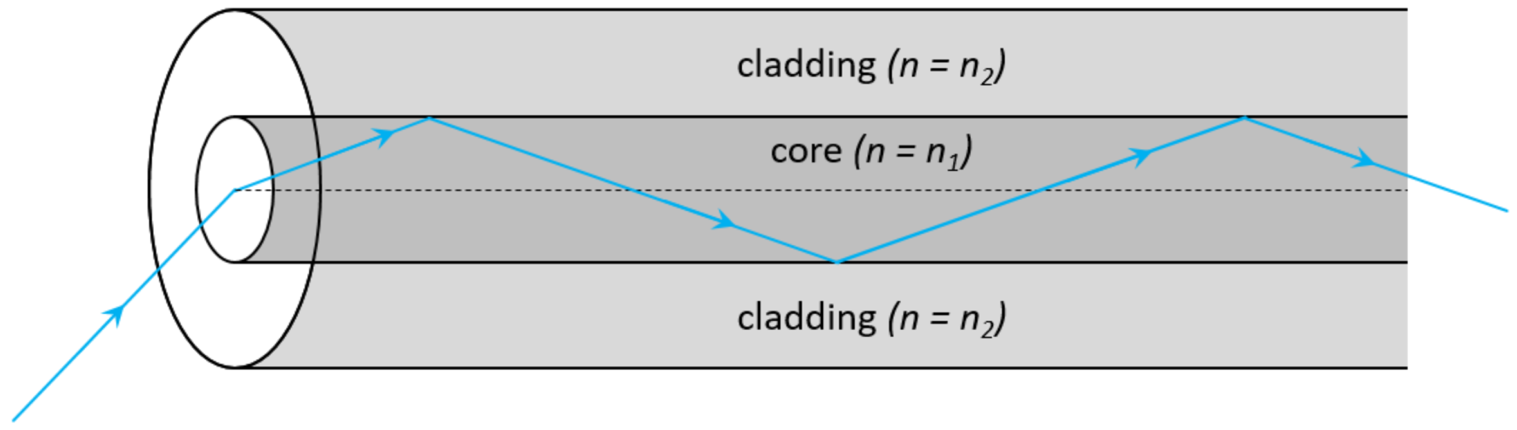
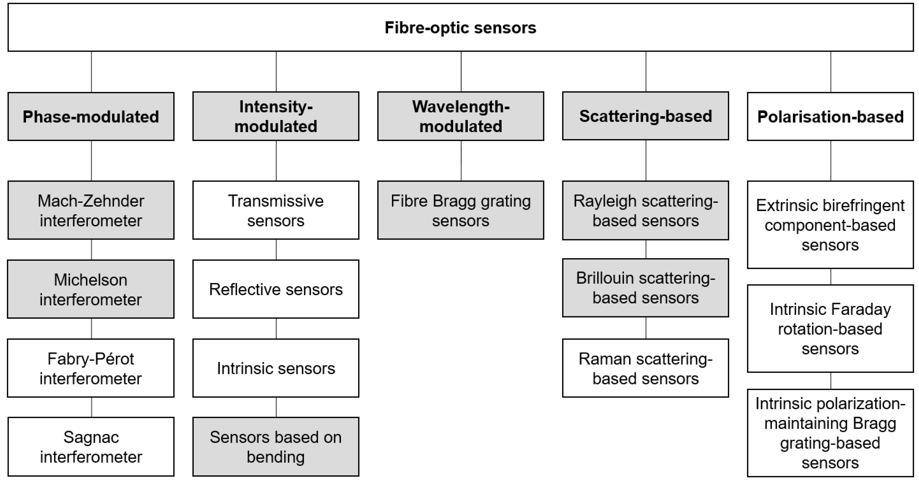
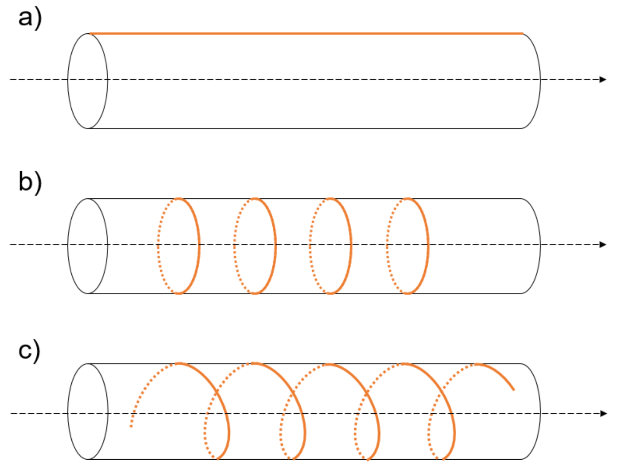
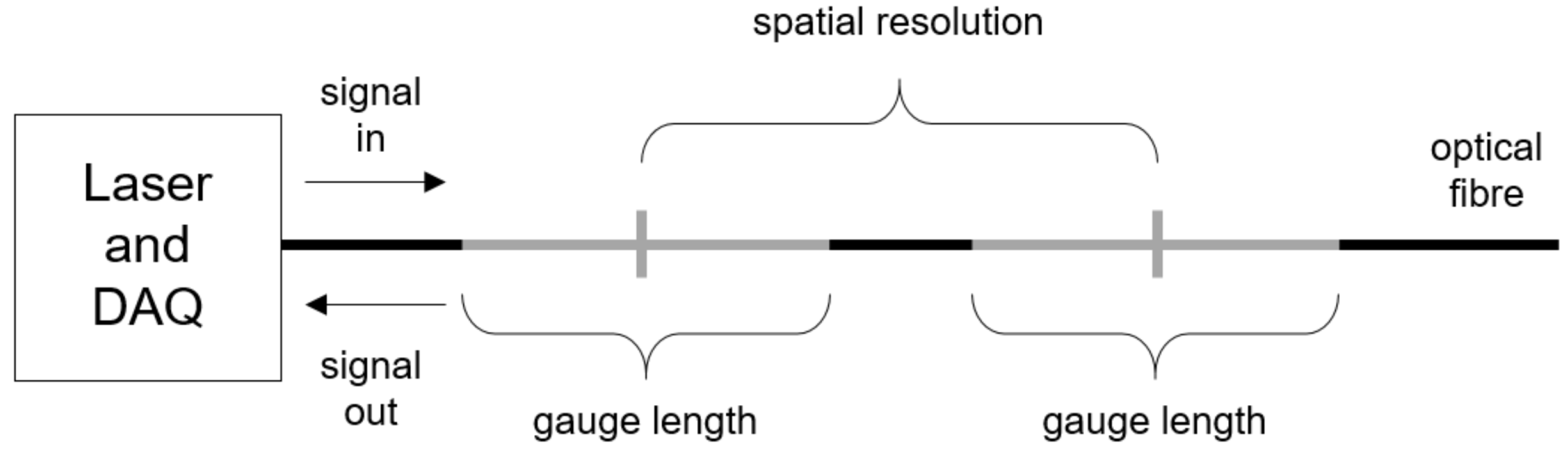
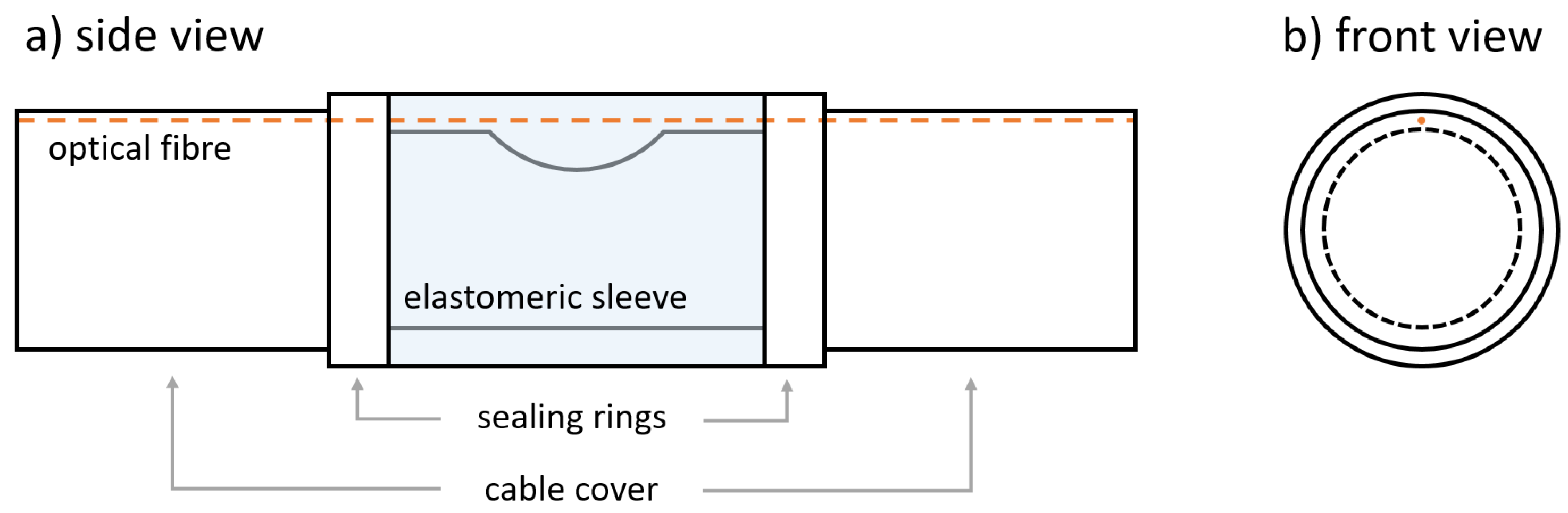
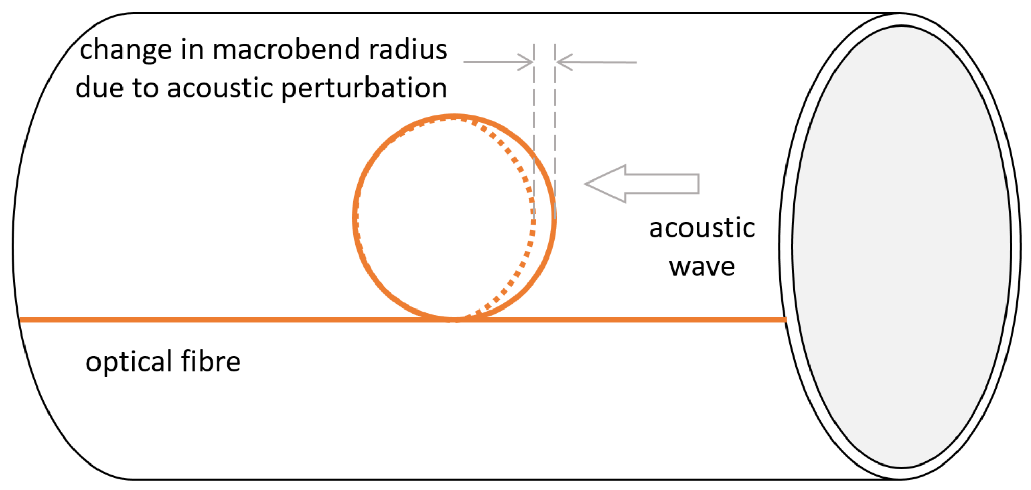
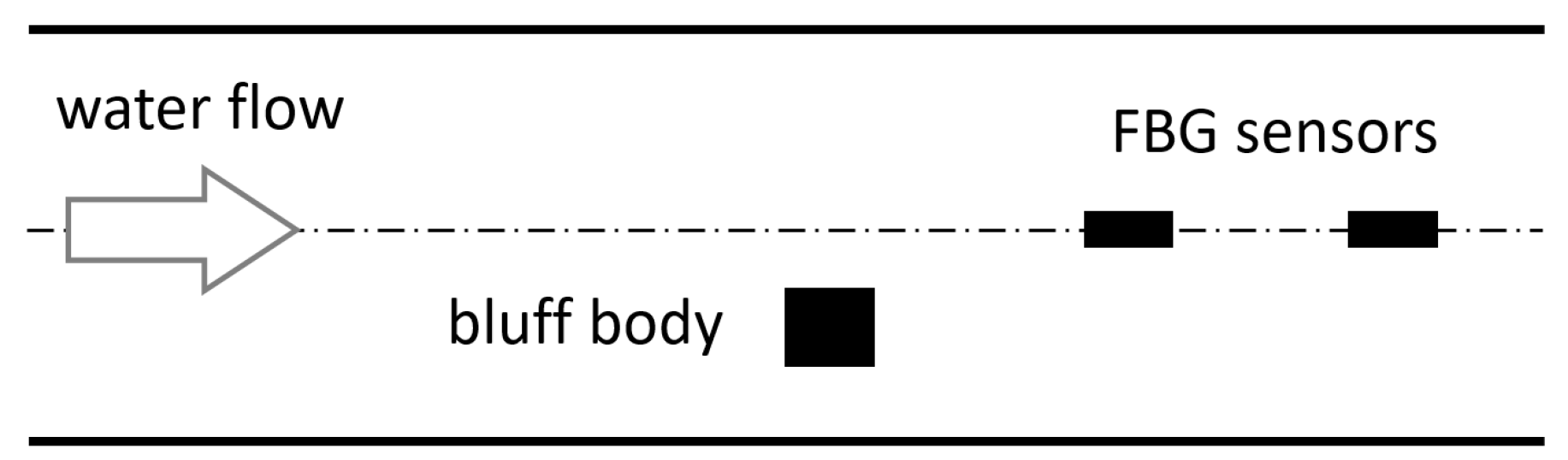
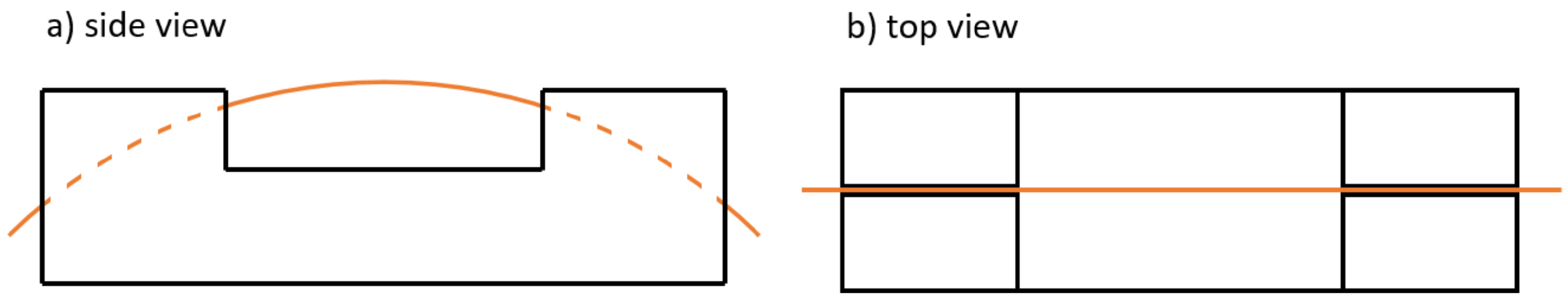
Table 1.
A selective summary of information presented in papers reviewed in Section 3. The figures in the brackets correspond to the numbers of related papers.
Table 1.
A selective summary of information presented in papers reviewed in Section 3. The figures in the brackets correspond to the numbers of related papers.
| Application | Method | Geometry | Retrofitting | Type of Environment | Validation |
|---|---|---|---|---|---|
| Condition monitoring (16) | Rayleigh OFDR (3) | Axial (9) | Easy (1) | Pressurised (10) | Lab (13) |
| BOTDR (3) | Hoop (4) | Moderate (1) | Non-pressurised (6) | Field (3) | |
| BOTDA (6) | Helical (2) | Difficult (14) | |||
| FBG (4) | Other (1) | ||||
| Leak detection (7) | Rayleigh OTDR (1) | Axial (1) | Easy (2) | Pressurised (7) | Lab (6) |
| Rayleigh OFDR (1) | Hoop (4) | Moderate (0) | Non-pressurised (0) | Field (1) | |
| FBG (3) | Helical (1) | Difficult (5) | |||
| Bend loss (1) | Other (1) | ||||
| Interferometry (1) | |||||
| Measurement of flow | Rayleigh OTDR (2) | Axial (3) | Easy (3) | Pressurised (7) | Lab (11) |
| parameters (12) | Rayleigh OFDR (2) | Helical (1) | Moderate (1) | Non-pressurised (5) | Field (2) |
| FBG (6) | Other (8) | Difficult (7) | Simulation (1) | ||
| Bend loss (1) | N/A (1) | ||||
| Interferometry (1) | |||||
| Total (35) | Rayleigh OTDR (3) | Axial (13) | Easy (6) | Pressurised (24) | Lab (30) |
| Rayleigh OFDR (6) | Hoop (8) | Moderate (2) | Non-pressurised (11) | Field (5) | |
| BOTDR (3) | Helical (4) | Difficult (26) | Simulation (2) | ||
| BOTDA (6) | Other (10) | N/A (1) | |||
| FBG (13) | |||||
| Bend loss (2) | |||||
| Interferometry (2) |
Publisher’s Note: MDPI stays neutral with regard to jurisdictional claims in published maps and institutional affiliations. |
© 2022 by the authors. Licensee MDPI, Basel, Switzerland. This article is an open access article distributed under the terms and conditions of the Creative Commons Attribution (CC BY) license (https://creativecommons.org/licenses/by/4.0/).
Share and Cite
MDPI and ACS Style
Prisutova, J.; Krynkin, A.; Tait, S.; Horoshenkov, K. Use of Fibre-Optic Sensors for Pipe Condition and Hydraulics Measurements: A Review. CivilEng 2022, 3, 85-113. https://0-doi-org.brum.beds.ac.uk/10.3390/civileng3010006
AMA Style
Prisutova J, Krynkin A, Tait S, Horoshenkov K. Use of Fibre-Optic Sensors for Pipe Condition and Hydraulics Measurements: A Review. CivilEng. 2022; 3(1):85-113. https://0-doi-org.brum.beds.ac.uk/10.3390/civileng3010006
Chicago/Turabian StylePrisutova, Jevgenija, Anton Krynkin, Simon Tait, and Kirill Horoshenkov. 2022. "Use of Fibre-Optic Sensors for Pipe Condition and Hydraulics Measurements: A Review" CivilEng 3, no. 1: 85-113. https://0-doi-org.brum.beds.ac.uk/10.3390/civileng3010006