An Analysis, Numerical Modeling and Experimental Verification of Low-Temperature Thermofoil Heaters

Abstract

In this paper, an analysis of the geometry, numerical modeling, and experimental verification of thermofoil heaters for low-temperature applications is presented. The research suggests a calculation procedure of the thermofoil traces’ geometry, comprising the necessary electrical and thermal parameters in order for the characteristics of the heater to be fully defined according to the stipulated conditions required. The derived heaters’ geometry analysis procedure is depicted with two case studies, giving the sequence of the necessary calculations and their applications as part of a design task. Its continuation, the design approach, is developed with numerical modeling, based on Finite Element Methods (FEM) used for multiphysics simulations, including the thermal and electrical heaters parameters. The realized 3D models are used to depict the uniformity of the thermal field in the system heatsink-thermofoil heater. The results from analysis, modeling, and simulations are tested experimentally. The suggested geometry analysis and modeling approach are experimentally verified. The final results demonstrate satisfactory precision with a simulation–experiment mismatch in a range of 5–7%. As a vital product of experimental research, the maximum power density for the studied thermofoil heaters is derived for a range of temperatures and material characteristics.

1. Introduction

Thermofoil heaters are used for low-temperature heating in a wide are of applications—industrial, domestic, automotive, telecommunications, military, aerospace, etc. Due to their specific flat geometry, these types of heaters ensure uniformly distributed temperature on a surface. The construction can be flexible or solid-state; customized according to the heated object (heatsink) shape, which leads to close assembling between the heater and the heatsink surfaces; low thermal resistance; and low thermal gradient. Low losses can be achieved by isolation from the ambience and hence high efficiency of the heating process, high thermal density and long-life expectancy; the possibility of integration with thermal sensors is a feasible requirement.

A vast amount of literature demonstrates the potential of flexible and solid-state low-temperature thermofoil heaters for industrial applications. Research focused on the vehicle battery systems [1] reveals inefficient battery cell operation at low ambient temperature under −20 °C, hence external low-temperature heating is necessary under such conditions. Although a specific heating system is not analyzed and designed as a case study at given battery parameters, this study suggests several possible constructions based on thermofoil heaters applied for cylindric and paunch li-ion cells. Another solution is based on Positive Temperature Coefficient (PTC) heaters [2], which is also an applicable technology for automotive applications, but the thermofoil heaters would ensure better distribution of the thermal field on the battery cells’ surface.

Other studies, based on flexible thin-film heaters, are focused on various applications such as automotive [3], sensors and displays [4], aircrafts [5], etc., show the necessity of thin-film heaters, which have the potential to be shaped according to the heatsink, producing a uniform thermal field. While some of the recent technologies are based on graphene and nanowires [6,7], which are still expensive for many applications, the thermofoil heaters have the potential to offer more appropriate budget-friendly engineering solutions, including copper-based traces in the micrometer range. The research in [8] is focused on the manufacturability of thin-film heaters in a micrometer range, where an approach for their resistance adjustments is presented. The presented heaters have a similar structure and geometry to the thermofoil heaters. The research also demonstrated that the current manufacturing technology can produce thermofoil heaters with a precision of tens of micrometers for heating of transparent surfaces, such as displays, with a precision sufficient enough for adjustment of the necessary resistance.

Another advance application of the thermofoil heaters is the possibility of their integration with different types of sensors, as numerous research publications present [9,10,11,12,13]. These studies prove the abilities of these types of heaters for integrating to a limited surface, where a low-temperature field must be uniformly distributed. The production and integration methods of heaters with transparent fundaments is analyzed in [9], and polyimide heater integration with a sensor is presented in [10]. A comprehensive research with sufficient data of heaters produced as part of a PCBs is presented in [11,12], but an analysis of the heater geometry and its placement on the heater surface is not developed, and this knowledge is not available in the public domain. A similar construction is used for flexible thin mm-sized resistance-typed sensor film in [13], but its design procedure is not presented. A throw research focused on solid-state and flexible thermofoil heaters would require the impact of the heater geometry over the thermal field to be analyzed according to the fundamental theory [14,15,16].

In the last several decades, thermal processes have been widely modeled and analyzed with Finite Element Methods (FEM), which is a proven approach for modeling of engineering processes and devices. These methods are widely used in numerous studies focused on thin-film and thermofoil heaters [17,18,19,20,21,22,23,24]. Conductive heat transfer between the heater layers is depicted in [17], and the applicable solvers for thermal analysis, electrical and Joule heating process, and the necessary mathematical model for thin-film heating are presented, respectively, in [18,19,20]. The heater position in horizontal and vertical direction is analyzed in [21,22], where models of the convection in different conditions are presented. Models of micro-electromechanical system (MEMS) with integrated thin-film heaters are an object of research in [23,24]. These papers present a limited amount of analysis of the heater geometry and its match to the heater surface according to the required power. Similarly, very limited details are available in the literature in relation to the procedure for determining the geometry of the models for modeling and simulation purpose. In this sense, an application of the fundamental theory [25,26,27] for thermal modeling and simulation, explicitly focused on the thermofoil heaters geometry parameters, is necessary to be further evolved. The development of such a practical design approach would improve the potential of thermofoil heaters in applications such as sensors, electronics, batteries, residential premises [28,29] and fluid heaters [30].

Significant amount of literature in this area highlights the potential applications for this type of heater. However, it is difficult to draw general conclusions from the literature for modelling and evaluating the design of heaters for future applications because of the knowledge gap in this area. The lack of proven methods for thermofoil heater geometry analysis can prevent further development and simulation work using FEM. This problem often leads to an application of the trial-and-error method on a bespoke basis simulation until the required geometry model is found.

Therefore, the aim of this research is to develop design procedures for achieving a uniform thermal field based on heater geometry analysis by numerical simulation. For this purpose, the necessary calculation procedures giving fully determined thermofoil heaters’ geometry will be developed. In this sense, the novelty of this research consists of its implementation in the analysis and the design procedure of the thermofoil flexible and solid-state low-temperature heaters. Its application produces an improved design and acceptable error between the results of simulation and experimental verification.

This paper is structured as follows: the suggested analysis of the heater’s geometry is presented in part two, supported with two case studies; part three gives its implementation in the numerical modeling and simulation; the experimental setup in part four provides experimental verification of the suggested analysis, providing a comparison between the results obtained from modeling and experiment; part five presents the summarized conclusions and recommendations for the design work.

2. Analysis of the Geometrical and Electrical Parameters of Thermofoil Heater

A generic characteristics geometry of the thermofoil considered for this analysis is shown in Figure 1. The fundamental equation relating to the geometry and electric parameters of the heaters can be used for modelling and simulation using FEM. The main geometry parameters are as follows: B is the heater stirp width; η is the isolation distance between the traces; ${\mathrm{L}}_{\mathrm{av}}$ is the average heater length; and H and W are, respectively, the overall height and width of the entire heater surface.

The resistance of a thin-film heater, comprised by N number of traces connected in parallel, can be derived by the electrical resistance equation as follows:

$${\mathrm{R}}_{\mathrm{th}}={\mathsf{\rho }}_{\mathrm{m}}\times \frac{{\mathrm{L}}_{\mathrm{av}}}{{\mathrm{A}}_{\mathrm{st}}}$$

(1)

where R_th is the thermofoil resistance (Ω), ρ_m is the specific resistance of the used material (Ωm), L_av is the average length (m) and A_st is the cross section of the heater (m²). It is assumed that all traces have equal cross-sections, which are a product of the width (B) and foil thickness (D) and can be calculated from A_st = D × B (m²).

The average length of the thermofoil heater L_av (m), comprised of N_st number of traces, is calculated from

$${\mathrm{L}}_{\mathrm{av}}={\mathrm{N}}_{\mathrm{st}}\times \left(\mathrm{H}+\mathsf{\eta }\right)\left(\mathrm{m}\right)$$

(2)

The heater’s power, along with the electric parameters R_th and ρ_m, depends on the geometric parameters B and D, and the overall heater’s borders W (Width), H (Height) shown in Figure 1. The calculated power of the heater P_th at given voltage V can be derived from $\mathrm{P}=\raisebox{1ex}{${\mathrm{V}}^2$}\!\left/ \!\raisebox{-1ex}{${\mathrm{R}}_{\mathrm{th}}$}\right.\left(\mathrm{W}\right)$ and Equation (1) as

$${\mathrm{P}}_{\mathrm{th}}=\frac{{\mathrm{V}}^2\times {\mathrm{A}}_{\mathrm{st}}}{{\mathsf{\rho }}_{\mathrm{m}}\times {\mathrm{L}}_{\mathrm{av}}}$$

(3)

The trace width B $\left(\mathrm{m}\right)$ depends on the overall sizes $\mathrm{W}$ and $\mathrm{H}$, and the specific resistance at given voltage $\mathrm{V}$ and heater power $\mathrm{P}$:

$$\mathrm{B}=\mathrm{k}\times \sqrt{{\left(\frac{\mathsf{\eta }}{2}\right)}^2+\frac{\mathrm{P}\times {\mathsf{\rho }}_{\mathrm{m}}\times \left(\mathrm{W}+\mathsf{\eta }\right)\times \mathrm{H}}{{\mathrm{V}}^2\times \mathrm{D}}}-\frac{\mathsf{\eta }}{2}$$

(4)

where $\mathrm{k}$ is a resizing factor.

In this research, the trace width is modified with a resizing factor $\mathrm{k},$ which ensures a better match between the geometrical and thermal parameters of the heater. The recommended values, a product of this research, are $\mathrm{k}=1.05$ for low resistance materials like copper and aluminum, and $\mathrm{k}=1.1$ for high-resistance alloys. The coefficient is experimentally derived at an average thermal rise over the ambient temperature of 60 °C and an average thermal conductivity of the isolation materials.

The number of the traces is calculated from

$${\mathrm{N}}_{\mathrm{st}}=\frac{\mathrm{W}}{\left(\mathrm{B}+\mathsf{\eta }\right)}$$

(5)

The trace with B $\left(\mathrm{m}\right)$ can be recalculated at round numbers for ${\mathrm{N}}_{\mathrm{st}\left(\mathrm{rnd}\right)}$ using

$${\mathrm{B}}_0=\frac{\mathrm{W}-\left({\mathrm{N}}_{\mathrm{st}\left(\mathrm{rnd}\right)}\times \mathsf{\eta }\right)}{{\mathrm{N}}_{\mathrm{st}\left(\mathrm{rnd}\right)}}$$

(6)

After the recalculation of the stirp width ${\mathrm{B}}_0$ with the rounded number ${\mathrm{N}}_{\mathrm{st}\left(\mathrm{rnd}\right)}$, the cross-section ${\mathrm{A}}_{\mathrm{st}}\left({\mathrm{m}}^2\right)$ will be

$${\mathrm{A}}_{\mathrm{st}}=\mathrm{D}\times {\mathrm{B}}_{\mathrm{o}}$$

(7)

and the heater power ${\mathrm{P}}_{\mathrm{th}}$, Equation (3), must be recalculated as well. Fill factor for parallel traces geometry ${\mathrm{FF}}_{\mathrm{ps}}$ is calculated from

$${\mathrm{FF}}_{\mathrm{ps}}=\frac{{\mathrm{B}}_{\mathrm{o}}\times \left(\mathrm{H}+\mathsf{\eta }\right)}{\mathrm{H}\times \left({\mathrm{B}}_{\mathrm{o}}+\mathsf{\eta }\right)}$$

(8)

At a targeted fill factor and given overall area of the heater (${\mathrm{A}}_{\mathrm{h}}=\mathrm{B}\times \mathrm{H}\left({\mathrm{m}}^2\right)$), the isolation distance η$\left(\mathrm{m}\right)$ between the traces can be calculated according to

$$\mathsf{\eta }=\frac{{\mathrm{A}}_{\mathrm{h}}\times \left(1-{\mathrm{FF}}_{\mathrm{ps}}\right)}{\left({\mathrm{FF}}_{\mathrm{ps}}\times \mathrm{H}\right)-\mathrm{B}}$$

(9)

After the rounding of the number of traces, ${\mathrm{N}}_{\mathrm{st}\left(\mathrm{rnd}\right)}$, a mismatch between the targeted power, given in the input parameters, and the calculated power from Equation (3) can be expected in order determine the relative error. It can be estimated as a relative error calculated from

$${\mathrm{p}}_{\mathrm{err}}=\left|\frac{{\mathrm{P}}_{\mathrm{th}}-\mathrm{P}}{\mathrm{P}}\right|\times 100\%$$

(10)

Due to the accepted resizing factors in Equation (4), the calculated error according to the last equation would always be positive in an expected range 5–10%. The purpose of this assumption is to minimize the mismatch between the model and experimental power. The minimization procedure is carried out using Equations (11) and (12).

The power density of the heater ${\mathrm{Q}}_{\mathrm{h}}\left(\frac{\mathrm{W}}{{\mathrm{m}}^2}\right)$ is described as the ratio between the heater nominal ${\mathrm{P}}_{\mathrm{n}}$ power and the heater surface ${\mathrm{S}}_{\mathrm{h}}$

$${\mathrm{Q}}_{\mathrm{h}}=\frac{{\mathrm{P}}_{\mathrm{th}}}{{\mathrm{S}}_{\mathrm{h}}}$$

(11)

where, the active surface ${\mathrm{S}}_{\mathrm{h}}$ $\left({\mathrm{m}}^2\right)$ is calculated from

$${\mathrm{S}}_{\mathrm{h}}=\left[{\mathrm{N}}_{\mathrm{st}}\times \left(\mathrm{H}\times \mathrm{B}\right)\right]+\left[\left({\mathrm{N}}_{\mathrm{st}}-1\right)\times \left(\mathrm{B}\times \mathsf{\eta }\right)\right]$$

(12)

The last two parameters can also be presented in squired centimeters (${\mathrm{cm}}^2$), which gives a better estimation considering the usual sizes of the thermofoil heaters. The recommended power density Q_h of the heater is experimentally verified in part 4.

As a final check, the calculated heater width ${\mathrm{W}}_{\mathrm{th}}$, considering the accepted ${\mathrm{N}}_{\mathrm{st}\left(\mathrm{rnd}\right)}$ and the trace width ${\mathrm{B}}_{\mathrm{o}}$ from

$${\mathrm{W}}_{\mathrm{th}}={\mathrm{N}}_{\mathrm{st}\left(\mathrm{rnd}\right)}\times \left({\mathrm{B}}_{\mathrm{o}}+\mathsf{\eta }\right)$$

(13)

must be smaller than the size $\mathrm{W}$ in the input parameters, i.e., ${\mathrm{W}}_{\mathrm{th}}<\mathrm{W}$, considering the given geometry tolerances. This ensures that the heater fits the required heater size. The uniform alignment of the stirps over the heater surface, after the rounding of the traces’ number, can be achieved with the resizing of the isolation gap $\mathsf{\eta }$. The final isolation gap between the traces will be ${\mathsf{\eta }}_{\mathrm{th}}$

$${\mathsf{\eta }}_{\mathrm{th}}=\mathsf{\eta }+\frac{\left(\mathrm{W}-{\mathrm{W}}_{\mathrm{th}}\right)}{\left({\mathrm{N}}_{\mathrm{st}\left(\mathrm{rnd}\right)}-1\right)}$$

(14)

The presented Equations (1)–(14) fully determine the thermofoil heater geometry, according to the most fundamental shape given in Figure 1. Their application and sequence of calculation are presented in the following case study.

Case study 1: preliminary design of the geometry of a thermofoil heater. The proposed preliminary design is conducted with the following input parameters: power of the designed thermofoil heater $\mathrm{P}=100\mathrm{W}$; width $\mathrm{W}=200\mathrm{mm}$; height $\mathrm{H}=200\mathrm{mm}$; voltage $\mathrm{V}=24\mathrm{V}$; isolation distance $\mathsf{\eta }=1\mathrm{mm}$; thermofoil thinness $\mathrm{D}=0.1\mathrm{mm}$. The calculations will be done with four different materials—cooper, aluminum, cooper-nickel, and chrome-nickel based alloys with a different specific resistance. The heater temperature is 60 °C at 20 °C ambient temperature. The results obtained from numerical analysis are shown in

Table 1. Results from case study 1.

Calculated Parameter	Equation	Thermofoil Heater Material
		Cooper	Aluminum	Cooper-Nickel Based Alloy	Chrome-Nickel Based Alloy
P = 100 W; W = 200 mm; H = 200 mm; V = 24 V; η = 1 mm; D = 0.1 mm
Specific resistance (Ω/m)	-	1.72 × 10−8	2.65 × 10−8	36.3 × 10 −8	2.35 × 10 −6
Trace width (B, mm)	4	0.74	1	4.79	16.28
Number of traces (Nst)	5	114.97	100.18	34.57	11.57
Rounded number of traces (Nst(rnd))	-	115	100	35	12
Recalculated trace width (Bo, mm)	6	0.74	1	4.71	15.67
Average length of the trace (Lav, m)	2	23.12	20.10	0.83	2.41
Thermofoil resistance (Rth, Ω)	1	5.38	5.33	5.43	5.16
Thermofoil cross-section (mm2)	7	0.07	0.1	0.47	1.57
Electric current through the heater (I, A)	I = V/R	4.46	4.51	4.43	4.65
Power of the heater (Pth, W)	3	107.08	108.14	106.33	111.68
Relative power error (|perr|, %)	10	7.08	8.14	6.33	11.68
Fill factor (FFps)	8	0.43	0.5	0.83	0. 9
Active surface of the heater (Sh, cm2)	12	170.84	200.99	332.60	377.72
Power density of the heater (Qh, W/cm2)	11	0.63	0.54	0.32	0.3
Heater width verification (Wth, mm)	13	85	100	165	188.00

.

The analysis of the results from the case study can be summarized as follows:

• The number of traces can vary in a wide range, in this case between 12 and 155, depending mainly on the specific resistance of the material. Hence, it is necessary for the suggested preliminary design to be conducted in order for the heater geometry to be determined at the given input parameters as a first approximation, i.e., before heater FEM modeling and simulation.
• The match between the power of the designed heater and the calculated power is satisfactory in a wide range of materials specific resistance. This result provides analytical verification of the consistency of Equation (4), as Equation (3) is calculated by the cross-section ${\mathrm{A}}_{\mathrm{st}}$, and, respectively, the thermofoil width $\mathrm{B}$ and its specified value ${\mathrm{B}}_0$. With this, a satisfactory match between the heater modeling and thermal simulation can be expected.
• For the chrome-nickel based alloy material, the specific resistance defers from the first three materials in a power of two. The calculated relative error is marginally over the assumed 10% error of the calculated power. In order for the precision to be improved, it can be recommended that the thickness of the foil can be increased 2 to 5 times, which lowers the foil width B, increases the foil length ${\mathrm{L}}_{\mathrm{av}}$ and the number of traces ${\mathrm{N}}_{\mathrm{st}}$ and eventually lowers the error ${\mathrm{p}}_{\mathrm{err}}$.
• The designed thermofoil heaters are oversized for the given power. An acceptable precision is achievable in the range of the fill factor ${\mathrm{FF}}_{\mathrm{ps}}=0.7-0.85$. The fill factor can be altered by varying the isolation distance η according to Equation (8). Additionally, it is a good design practice for $\mathsf{\eta }$ to be accepted as little as possible at the beginning of the design procedure, as it will be resized after the final number of traces is calculated.

3. Analysis of the Power Density

In this research, the steady-state heaters are produced by Printed Circuit Board (PCB) for experimental work. The maximum power density is experimentally tested for low-voltage flexible thermofoil and steady-state heaters, based on several types of thermal and electrical insulators between the thermofoil and the heatsink surface. The experimental data is used to derive empirical equations, producing an estimation of the maximum permitted power density. The experiments are conducted with heaters in a low-temperature range up to 120 °C, power in the range of $5\mathrm{W}$ to $1000\mathrm{W}$, and surface between $5{\mathrm{cm}}^2$ and $5000{\mathrm{cm}}^2$.

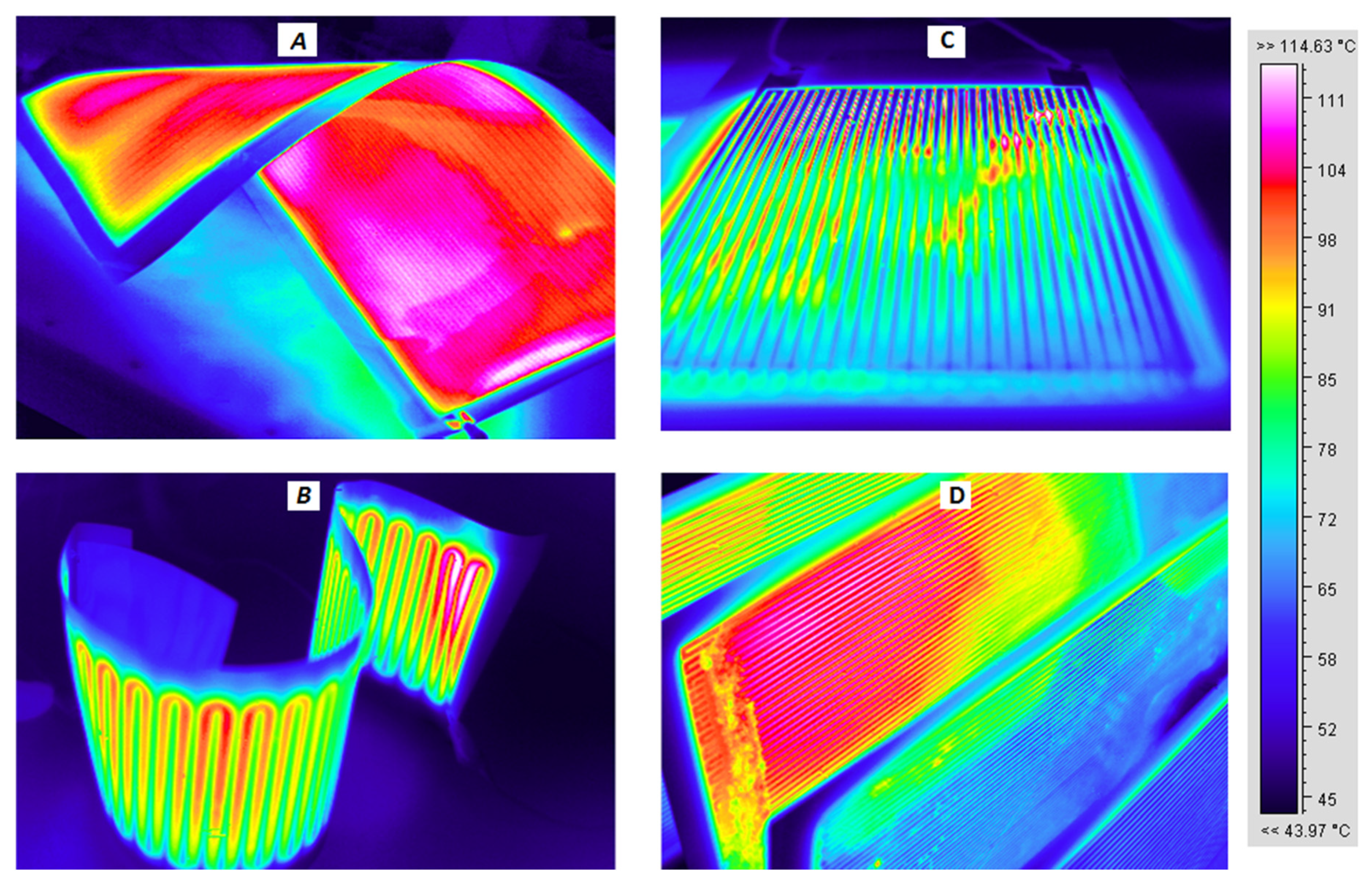
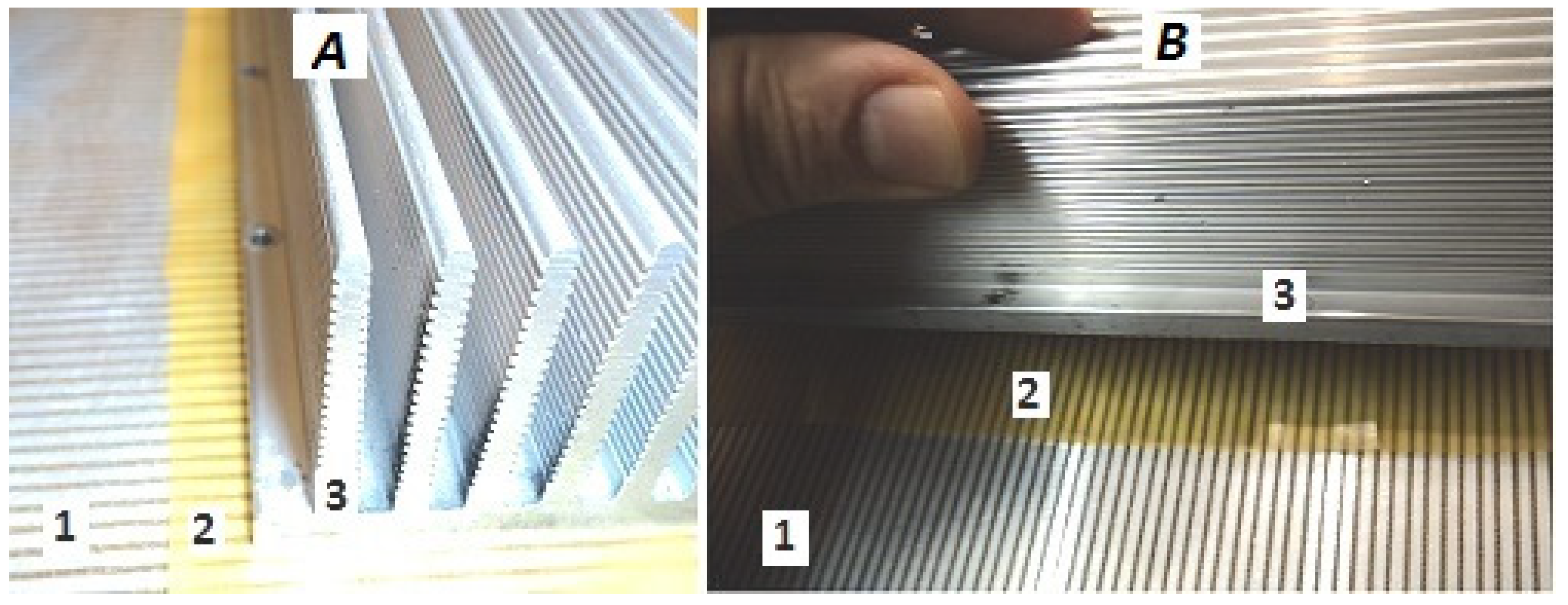
Figure 2 shows infrared images of several models of flexible and PCB heaters, object of experimental verification, and Figure 3 shows the mounting method of PCB heater. The experiments are done with both heaters assembled to a heatsink with external cooling, electrically insulated by a thermal conductive material. The temperature is measured at the surface of the heater and the surface of the heatsink; the transient thermal process is compared to results from modeling in part 5.

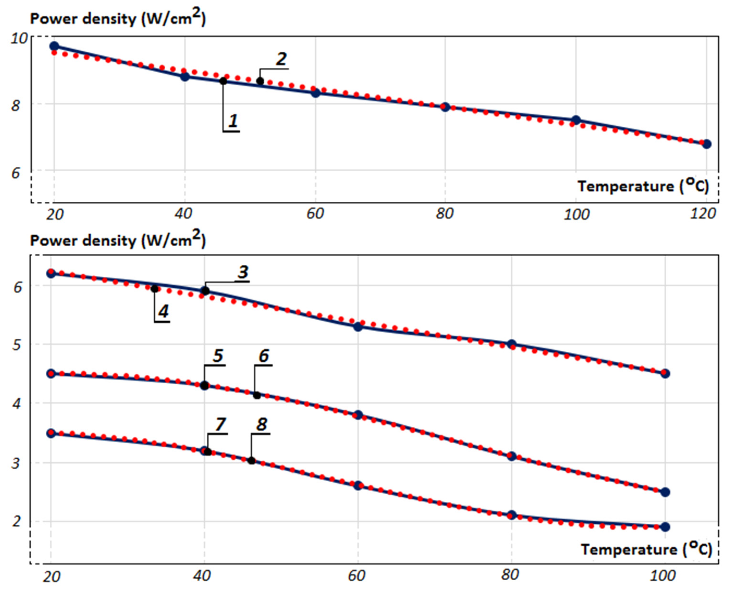
The experimentally obtained results, showing the maximum power density ${\mathrm{Q}}_{\mathrm{h}}$ as a functional dependency of the heated object temperature, in the low-temperature range 20–100 °C, are presented in Figure 4 as follows: graphic 1 shows a flexible thermofoil heater, comprised of aluminum traces and mica and its linearization in graphic 2; graphics 3 and 4, respectively, PCB heater with mica and its linearization; graphics 5 and 6 PCB heater with silicone rubber; and graphics 7 and 8 PCB heater with thermal proved fabric.

For all experimentally obtained graphics 1, 3, 5 and 7 are derived equations according to the dashed linearization graphics 1 and 4 and the trend lines 6 and 7, in order for the selection precision to be improved. E.g., for the flexible cooper-mica heater (graphic 2), the power density ${\mathrm{Q}}_{\mathrm{h}}$ at a temperature $\mathrm{T}$ in the range between 20 °C and 120 °C can be calculated from

$${\mathrm{Q}}_{\mathrm{h}}=-0.0269\mathrm{T}+10.047$$

(15)

and, respectively, for the PCB heater (graphic 4) in the temperature range between 20 °C and 100 °C from the equation

$${\mathrm{Q}}_{\mathrm{h}}=-0.0215\mathrm{T}+6.67$$

(16)

The experimental graphics 5 and 7 have a more complex shape, and their linearization would give unsatisfactory precision. In this case, polynomial equations would offer better results. Because of that, two third-degree polynomial equations are derived, shown with dashed graphics 6 and 8, which, respectively, follow the shape of the experimental graphics 5 and 7. With this, the polynomial equations giving the power density ${\mathrm{Q}}_{\mathrm{h}}$ for diagram 5 are

$${\mathrm{Q}}_{\mathrm{h}}=4\times {\mathrm{E}}^{-6{\mathrm{T}}^3}-0.0009\times {\mathrm{T}}^2+0.0348\times \mathrm{T}+4.14$$

(17)

and for diagram 7 are

$${\mathrm{Q}}_{\mathrm{h}}=6\times {\mathrm{E}}^{-6{\mathrm{T}}^3}-0.0011\times {\mathrm{T}}^2+0.0311\times \mathrm{T}+3.26$$

(18)

According to the experimentally obtained dependencies, the heaters designed in case study 1 are oversized, as the power density is strongly under the potential power density for the suggested surface. Case study 2 aims to show an improvement of the presented preliminary geometry design for materials copper and aluminum, finding a solution with the maximum power density.

Case study 2: preliminary geometry design, based on the maximum power density of the PCB heater. The case study 2 is a continuation of the case study 1, conducted for the copper and aluminum, based on the experimentally verified power density, graphic 7, Figure 4. In this case study, the presented power density is included. For the case of thermal proved fabric, at $2\left(\mathrm{W}/{\mathrm{cm}}^2\right)$ with an accepted safety margin, and the above given H and W sizes, the heater power can be increased to 800 W. The obtained results are depicted in

Table 2. Results from case study 2.

Calculated Parameter	Equation	Thermofoil Heater Material
		Cooper	Aluminum
2 (W/cm2), P = 800 W
Specific resistance (Ω/m)	-	1.72 × 10−8	2.65 × 10−8
Trace width (B, mm)	4	2.77	3.55
Number of traces (Nst)	5	53.04	43.97
Rounded number of traces (Nst(rnd))	-	53	44
Recalculated trace width (Bo, mm)	6	2.77	3.55
Average length of the trace (Lav, m)	2	10.65	8.84
Thermofoil resistance (Rth, Ω)	1	0.66	871.36
Thermofoil cross-section (mm2)	7	0.28	0.35
Electric current through the heater (I, A)	I = V/R	36.33	36.31
Power of the heater (Pth, W)	3	871.89	871.36
Relative power error (|perr|, %)	10	8.99	8.92
Fill factor (FFps)	8	0.74	0.78
Active surface of the heater (Sh, cm2)	12	295.44	313.52
Power density of the heater (Qh, W/cm2)	11	2.95	2.78
Heater width verification (Wth, mm)	13	147	156

.

The presented calculations show better power density at the given power and heater sizes. The active surface area, according to the calculated trace width, fits the heater size, which on the design level shows a better possibility the heater to be modeled, prototyped and experimentally tested.

4. Numerical Modeling of Thermofoil Heaters

The geometry of the thermofoil heater analysis determines all of the necessary sizes with satisfactory precision in order for the geometry model to be produced and initialized in the simulation procedure. As the heat transfer is a complex process [25,26,27], its time-depended modeling, calculating the transient heat-up process, requires significant computer resurges for 3D models. In this part, a simplified FEM model is proposed [31,32,33], considered with the specific thermofoil characteristics and heat transfer in the system thermofoil heater-heatsink, realized by specialized software COMSOL multiphysics [34,35]. The aim of such simplification is to make 3D simulation procedures feasible for acceptable time and computer resources, without decreasing their precision. Due to this requirement, its validity is experimentally verified in the next point.

(A) Thermal model

The thermal model is developed with the following assumption: the direction of the thermal flux is from the theater toward the heat sink, i.e., the heater is isolated from the ambient environment. The only media between the thermofoil and the heat sink—the insulation material—is assembled with a precise match between both surfaces; the convection and irradiation from the thermofoil heater surfaces to the ambient are neglected, as they are completely isolated in this direction.

The heat transfer between the thermofoil heater and the heatsink is defined by the equation

$${\mathsf{\rho }\mathrm{C}}_{\mathrm{p}}\frac{\partial \mathrm{T}}{\partial \mathrm{t}}+{\mathsf{\rho }\mathrm{C}}_{\mathrm{p}}\mathrm{u}.\nabla \mathrm{T}+\nabla .\mathrm{q}=\mathrm{Q}$$

(19)

$$\mathrm{q}=-\mathrm{k}.\nabla \mathrm{T}$$

(20)

where $\mathsf{\rho }$ is the material density ($\mathrm{kg}/{\mathrm{m}}^3$); ${\mathrm{C}}_{\mathrm{p}}$ is the heat capacity $\left(\mathrm{J}/\left(\mathrm{kg}.\mathrm{K}\right)\right)$; $\mathrm{T}$ is the temperature $\left(\mathrm{K}\right)$; $\mathrm{u}$ is the velocity field vector $\left(\mathrm{m}/\mathrm{s}\right)$; Q is the heat source $\left(\mathrm{W}/{\mathrm{m}}^3\right)$; q is the heat flux vector $\left(\mathrm{W}/{\mathrm{m}}^2\right)$; and $\mathrm{k}$ is the conductivity $\left(\mathrm{W}/\left(\mathrm{m}.\mathrm{K}\right)\right)$.

The boundary condition for thermal insulation is described as

$$-n.\mathrm{q}=0$$

(21)

where n is the vector potential.

The convective heat flux ${\mathrm{q}}_0\left(\mathrm{W}/{\mathrm{m}}^2\right)$ from the heat sink surface to the ambient is given by

$$-n.\mathrm{q}={\mathrm{q}}_0=\mathrm{h}\left({\mathrm{T}}_{\mathrm{amb}}-\mathrm{T}\right)$$

(22)

where h (W/m²C) is the convective heat transfer (depending the type of the convection), the surface and its orientation; T_amb is the ambient temperature.

The radiation from the heatsink surface q_i toward the ambient environment is described by

$$-n.\mathrm{q}={\mathrm{q}}_{\mathrm{i}}=\mathsf{\epsilon }\mathsf{\sigma }\left({\mathrm{T}}_{\mathrm{amb}}^4-{\mathrm{T}}^4\right)$$

(23)

where ε is the material emissivity and σ is the Stefan–Boltzmann constant.

(B) Thermal model

The Joule heating model describes the heating of the electrical conductor from the electric current passing through it due to the Joule losses. The equation describing the dependency between the conductivity of the material (in this case, the thermal foil and its temperature) is

$$\mathsf{\sigma }=\frac{1}{{\mathsf{\rho }}_0\left(1+\mathsf{\alpha }\left(\mathrm{T}-{\mathrm{T}}_0\right)\right)}$$

(24)

where ρ₀ is the resistivity, α is the resistivity temperature coefficient and T and T₀ are the current temperature and the reference temperature.

The external current density J appears in Ohm’s law and is described by the following equations:

$$\nabla .\mathrm{J}={\mathrm{Q}}_{\mathrm{j}}$$

(25)

$$\mathrm{J}=\mathsf{\sigma }.\mathrm{E}+\frac{\partial \mathrm{D}}{\partial \mathrm{t}}+{\mathrm{J}}_{\mathrm{e}}$$

(26)

$$\mathrm{E}=-\nabla \mathrm{V}$$

(27)

Eventually, the current conservation is

$$\mathrm{J}=\left(\mathsf{\sigma }+{\mathsf{\epsilon }}_{\mathrm{o}}{\mathsf{\epsilon }}_{\mathrm{r}}\frac{\partial }{\partial \mathrm{t}}\right).\mathrm{E}+{\mathrm{J}}_{\mathrm{e}}$$

(28)

where J_e is external current density $\left(\frac{\mathrm{A}}{{\mathrm{m}}^2}\right)$; ε₀, ε_r are the permittivity of the free space and relative permittivity, respectively; and ${\mathrm{Q}}_{\mathrm{J}}\left(\frac{\mathrm{A}}{{\mathrm{m}}^2}\right)$ is current source, described by equation

$${\mathrm{Q}}_{\mathrm{j}}=\mathrm{n}.\left({\mathrm{J}}_1-{\mathrm{J}}_2\right)$$

(29)

The electric isolation boundary condition means that no electric current flows through the boundary, i.e., the current leakage between the thermofoil and the heatsink is neglected

$$\mathrm{n}.\mathrm{J}=0$$

(30)

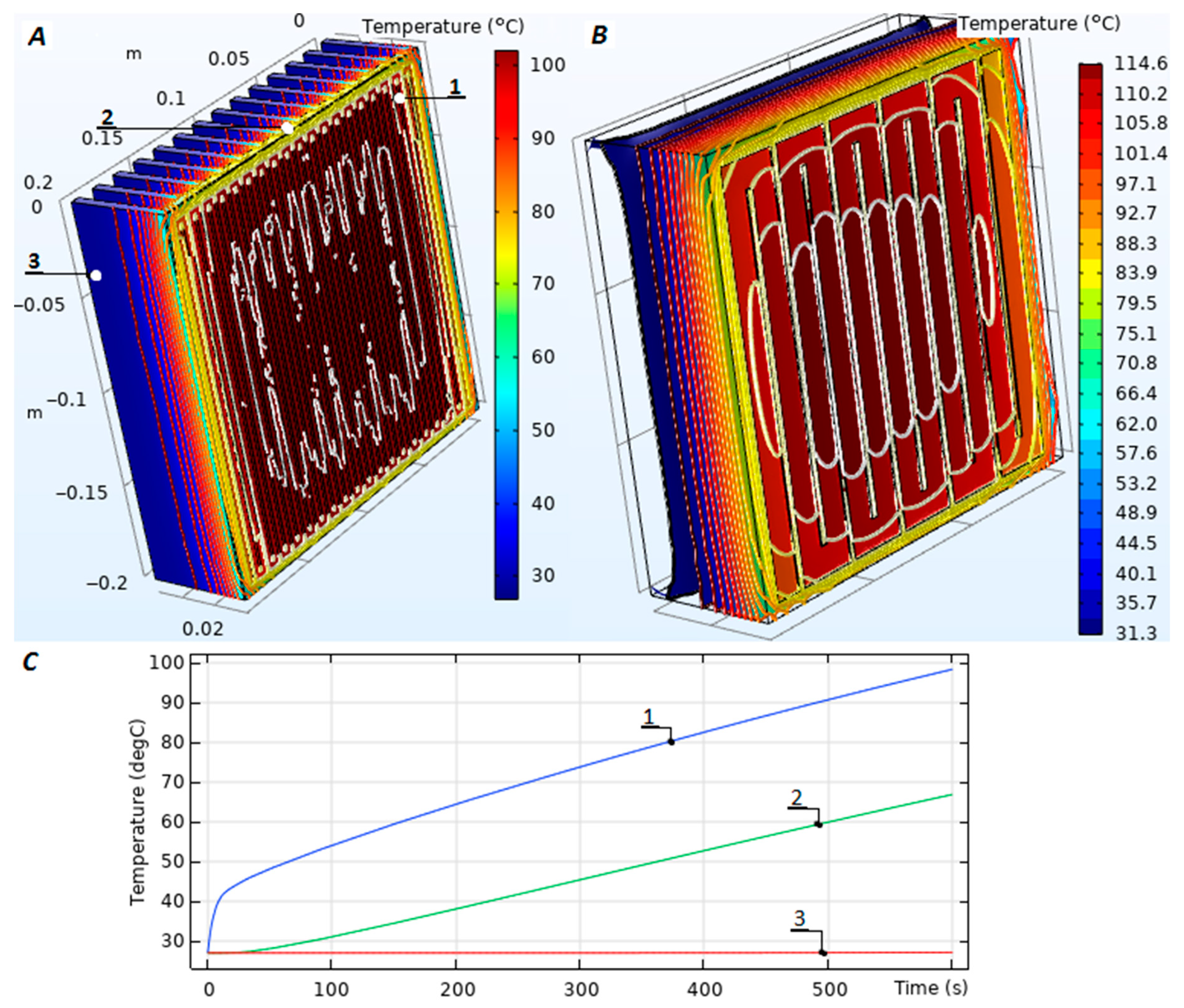
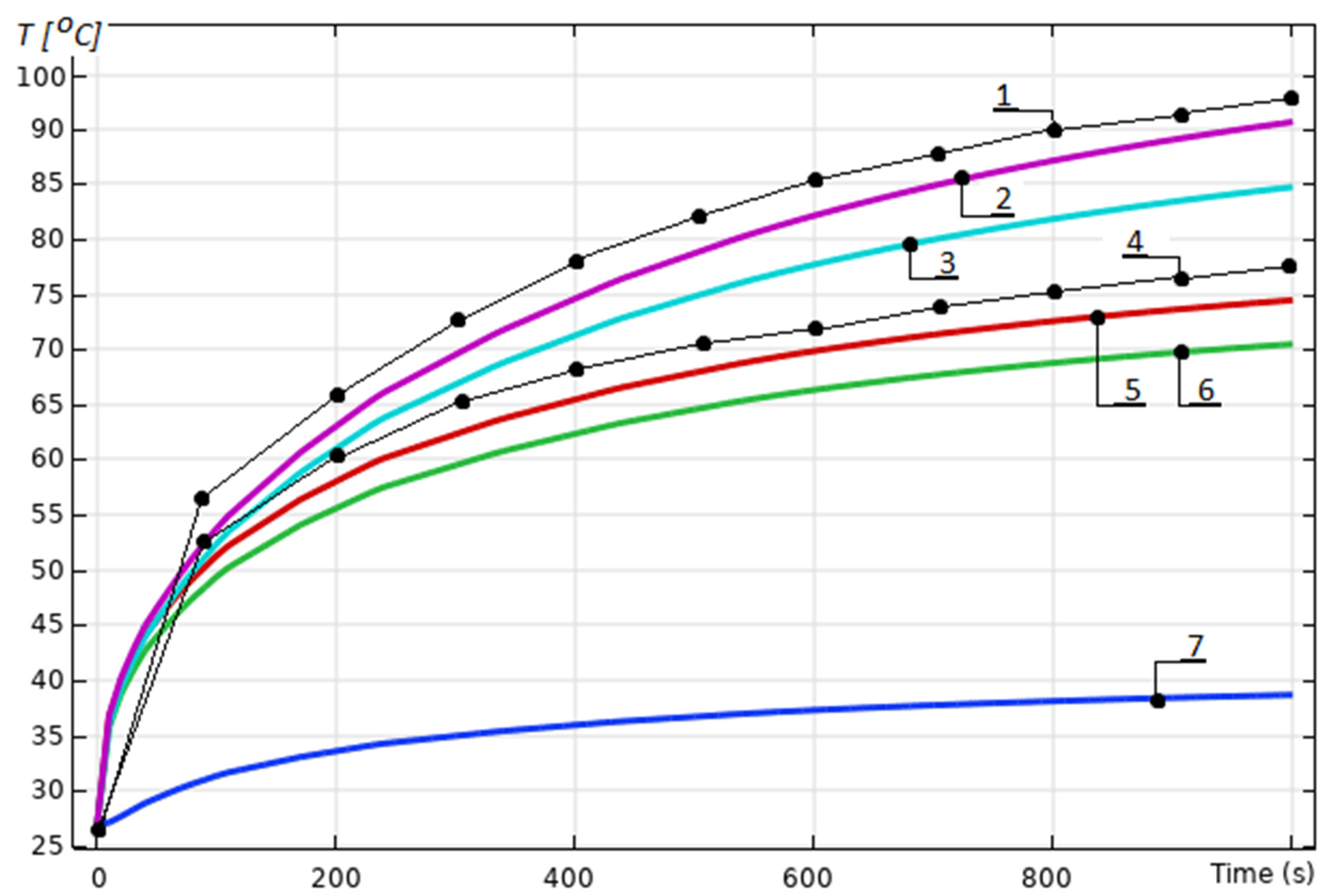
Figure 5 shows 3D models of thermofoil heaters with conducted multiphysics simulation, comprised of thermal model, Equations (19)–(23), and electric model, Equations (24)–(30). The geometry model parameters B, H, W, $\mathsf{\eta }$, D, ${\mathrm{N}}_{\mathrm{st}}$, ${\mathrm{L}}_{\mathrm{av}}$ and ${\mathrm{S}}_{\mathrm{h}}$ are calculated according to Equations (1)–(14), and the ${\mathrm{Q}}_{\mathrm{h}}$ is calculated according to Equation (18). As a final result, the transient process for the model given in Figure 5A is shown in Figure 5C. Graphic 1, Figure 5, shows the temperature of the heater; graphic 2 the temperature of the heatsink on the surface between two ribs; and graphic 3 shows the temperature at the end of the rib maintaining constant in order for the maximum power density to be estimated (Figure 3 and Figure 4). The transient heating process depends on the heatsink thermal capacity and heater power. It is described analytically with the equation:

$$\mathrm{P}=\frac{{\mathrm{mC}}_{\mathrm{p}}∆\mathrm{T}}{\mathrm{t}}$$

(31)

where P is the power in watts, ∆T is the thermal difference between the initial temperature T_ini and the final temperature T_f of the heatsink, i.e., $∆\mathrm{T}={\mathrm{T}}_{\mathrm{ini}}-{\mathrm{T}}_{\mathrm{f}}$ (°C); $\mathrm{m}$ (grams) is the mass of the heatsink, obtained from the material density and volume; $\mathrm{t}$(sec) is the time; and $\mathrm{C}$ is the heat capacity as it is shown in Equation (18). Respectively, the necessary time in seconds that the temperature ${\mathrm{T}}_{\mathrm{f}}$ needs to reach is

$$\mathrm{t}=\frac{{\mathrm{mC}}_{\mathrm{p}}∆\mathrm{T}}{\mathrm{P}}$$

(32)

Another analysis based on modeling and simulation, giving the distribution on the thermal field presented in Figure 6. The impact of the geometry over the shape of the thermal field can be numerically verified, as it is depicted with the presented examples: in Figure 6A, with trace width $\mathrm{B}=20\mathrm{mm}$ (Equation (6)) and insulation gap $\mathsf{\eta }=50\mathrm{mm}$ (Equation (14)), the thermal difference on the heatsink surface is 61.5 °C; in Figure 6B, respectively, $\mathrm{B}=60\mathrm{mm}$ and $\mathsf{\eta }=10\mathrm{mm}$ and the thermal difference is 12.2 °C; in Figure 6C $\mathrm{B}=68\mathrm{mm}$ and $\mathsf{\eta }=2\mathrm{mm}$ and the thermal difference is 0.2 °C.

5. Experimental Verification of the Thermal Field and Simulation-Experimental Data Comparison

The experimental verification is supported by a series of experiments to compare and to confirm the results obtained from geometry design, Equations (1)–(14). The power density is considered according to the experimental graphics depicted in Figure 4 and the derived Equations (15)–(17). A difference under 10% can be accepted as successful, justifying the suggested design approach and FEM modeling simplification for the studied thermofoil heaters.

Figure 7 presents the experimental verification of the transient heating up-process, described by Equations (31) and (32). Graphic 1 shows the temperature measured over the copper traces of the thermofoil heater. The difference with the FEM simulation showed with graphic 2 is in the acceptable range of 5–7%. The same graphic is obtained from the 3D model shown in Figure 7 with a geometry model designed according to the Equations (1)–(14). In this verification, the recommended coefficients $\mathrm{k}$ in Equation (4) are also included in the parameters’ calculations. Without such a correction, a simulation conducted with a recalculated geometry model gives graphic 3 with an error of over 10%. The result confirms the variability of the included width trace increase and power increase on the design level of 5–10.

The transient process on the surface of the heatsink (Figure 5, point 2) shows the same dependence as the experimental measurements depicted in graphic 4; the simulations given in graphic 5, according to Equation (4); and the simulations in graphic 6, without the necessary geometry correction. Graphic 7 shows the temperature in the middle of the heat sink’s rib obtained from the FEM simulation.

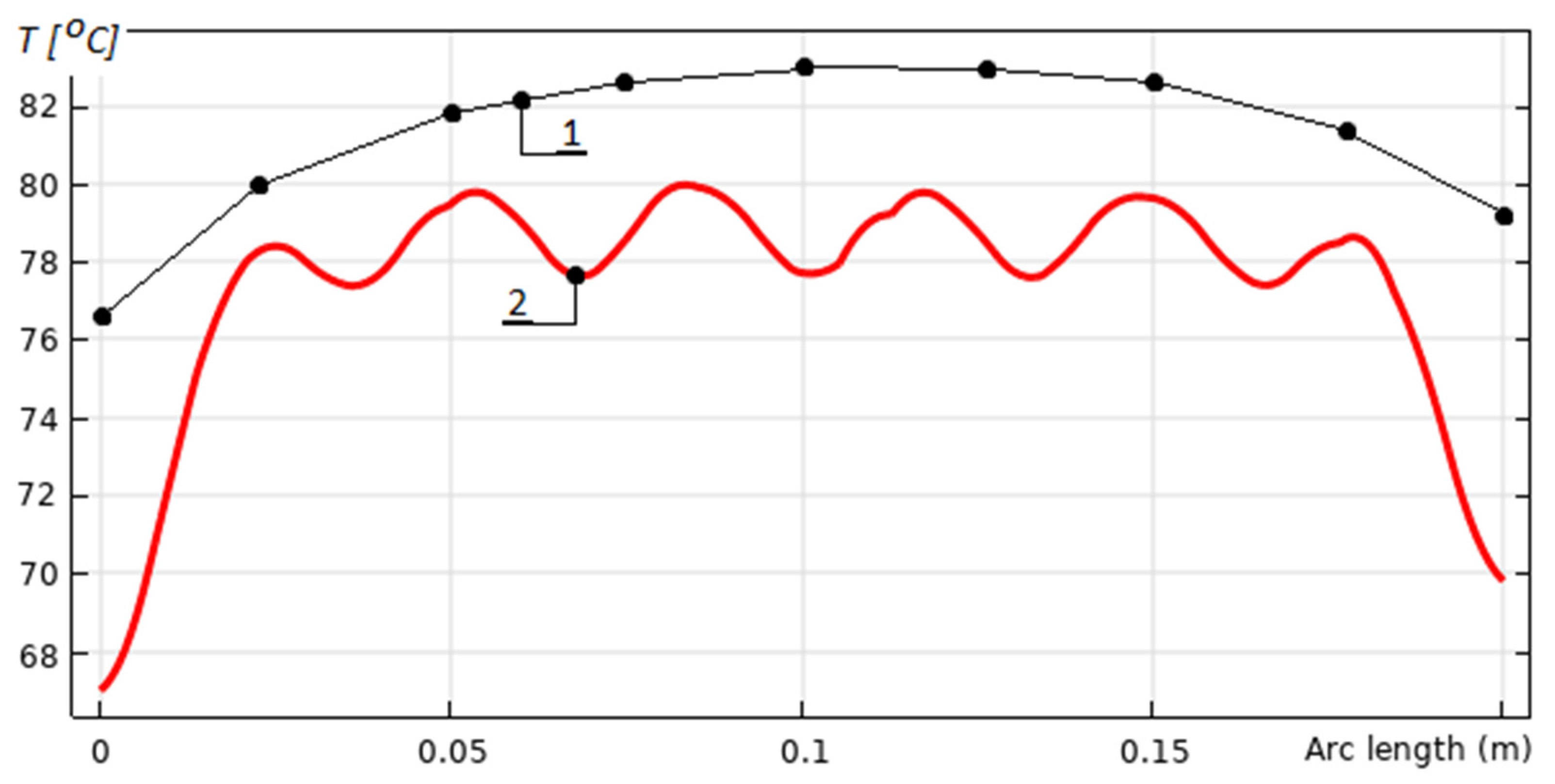
Figure 8 presents experimental verification of the temperature distribution on the heatsink surface. Graphic 1 shows the experimental measurements at the final point (900 s) of graphic 1, Figure 7, with a temperature drop of 12–15 °C, due to the thermal insulation and the distance from the thermofoil traces. The comparison shows an acceptable average error of 3–7% in the central part of the heater where the convection heat exchange from the ambient is minimized. In some cases, the mismatch reaches more than 10–15% only at the heatsink edges, which generally does not disturb the overall design precision.

6. Conclusions

In this paper, an analysis of the geometry, numerical modelling, and experimental verification of low-temperature thermofoil heaters have been presented.

The thermofoil geometry, presented in Figure 1, has been completely determined with the derived Equations (1)–(14), supported with two case studies. The suggested methodology has been designed in order for the thermofoil parameters—the number of traces, width, average length, resistance, fill factor, and active area—to be calculated. A geometry correction coefficient in Equation (4) has been suggested in order for the precision of the design and modelling procedure to be improved. The result is experimentally verified and depicted in Figure 7 graphics 1–6.

The maximum power density, as a starting point of the thermofoil heaters design, has been determined experimentally (Figure 2 and Figure 3) for a wide power range of thermofoil heaters, and the results have been summarized graphically and analytically in Figure 4 and Equations (15)–(18). Although the presented results strongly depend on the heater geometry, assembling the heatsink and insulator thermal parameters, they are applicable as a first approximation for a wide range of design tasks.

The results from the suggested FEM modelling, Equations (19)–(30), based on idealized thermal and electrical models have been experimentally verified. The modelling-experimental verification mismatch is acceptable in a range of 5–7%. With this, the final comparison (Figure 7 and Figure 8) confirms experimentally the consistency of the suggested design approach.

The presented results can successfully be applied for the design of low-temperature, flexible and solid-state thermofoil heaters for varies purposes. Future research suggests improvements in terms of modelling, different shapes of surfaces that require flexible heaters, specific applications, etc.

References

- Hu, X.; Zheng, Y.; Howey, D.; Perez, H.; Foley, A.; Pecht, M. Battery Warm-up Methodologies at Subzero Temperatures for Automotive Applications: Recent Advances and Perspectives. Prog. Energy Combust. Sci. 2020, 77, 100806. [Google Scholar] [CrossRef]
- Shin, Y.; Sim, S.; Kim, S. Performance Characteristics of a Modularized and Integrated PTC Heating System for an Electric Vehicle. Energies 2016, 9, 18. [Google Scholar] [CrossRef] [Green Version]
- Sun, J.; Yu, X.; Li, Z.; Zhao, J.; Zhu, P.; Dong, X.; Yu, Z.; Zhao, Z.; Shi, D.; Wang, J.; et al. Ultrasonic Modification of Ag Nanowires and Their Applications in Flexible Transparent Film Heaters and SERS Detectors. Materials 2019, 12, 893. [Google Scholar] [CrossRef] [Green Version]
- Zhang, Y.; Liu, H.; Tan, L.; Zhang, Y.; Jeppson, K.; Wei, B.; Liu, J. Properties of Undoped Few-Layer Graphene-Based Transparent Heaters. Matererials 2019, 13, 104. [Google Scholar] [CrossRef] [Green Version]
- Vertuccioa, L.; Santisa, F.; Pantania, R.; Lafdib, K.; Guadagnoa, L. Effective De-icing Skin Using Graphene-Based Flexible Heater. Compos. Part B 2019, 162, 600–610. [Google Scholar] [CrossRef]
- Kim, Y.J.; Kim, G.; Kim, H.-K. Study of Brush-Painted Ag Nanowire Network on Flexible Invar Metal Substrate for Curved Thin Film Heater. Metals 2019, 9, 1073. [Google Scholar] [CrossRef] [Green Version]
- Zhang, C.; Liang, S.; Zhu, H.; Wang, W. Tunable DFB lasers integrated with Ti thin film heaters fabricated with a simple procedure. Opt. Laser Technol. 2013, 54, 148–150. [Google Scholar] [CrossRef] [Green Version]
- Scorzonia, A.; Tavernellia, M.; Placidia, P.; Valigia, P.; Zampollib, S.; Caputoc, D.; Petruccic, G.; Nascettic, A. Improvement of the Thermal Resistance of Thin Film Heaters on Glass Substrate for Lab-On-Chip Applications. Procedia Eng. 2014, 87, 959–962. [Google Scholar] [CrossRef] [Green Version]
- Caputoa, D.; Parisi, E.; Nascetti, A.; Mirasoli, M.; Nardecchia, M.; Lovecchio, N.; Petrucci, G.; Costantini, F.; Roda, A.; Cesare, G. Integration of Amorphous Silicon Balanced Photodiodes and Thin Film Heaters for Biosensing Application, 30th Eurosensors Conference, EUROSENSORS 2016. Procedia Eng. 2016, 168, 1434–1437. [Google Scholar]
- Suganuma, Y.; Sasaki, M.; Nakayama, T.; Muroyama, M.; Nonomura, Y. Cu Thin Film Polyimide Heater for Nerve-Net Tactile Sensor. Proceedings 2017, 1, 303. [Google Scholar] [CrossRef] [Green Version]
- Hintermüller, M.; Offenzeller, C.; Knoll, M.; Tröls, A.; Jakoby, B. Parallel Droplet Deposition via a Superhydrophobic Plate with Integrated Heater and Temperature Sensors. Micromachines 2020, 11, 354. [Google Scholar] [CrossRef] [PubMed] [Green Version]
- Pawlak, R.; Lebioda, M. Electrical and Thermal Properties of Heater-Sensor Microsystems Patterned in TCO Films for Wide-Range Temperature Applications from 15 K to 350 K. Sensors 2018, 18, 1831. [Google Scholar] [CrossRef] [PubMed] [Green Version]
- Xu, Z.; Fan, Y.; Wang, T.; Huang, Y.; Dehkordy, F.; Dai, Z.; Xia, L.; Dong, Q.; Bagtzoglou, A.; McCutcheon, J.; et al. Towards High Resolution Monitoring of Water Flow Velocity Using Flat Flexible Thin mm-Sized Resistance-Typed Sensor Film (MRSF). Water Res. X 2019, 4, 100028. [Google Scholar] [CrossRef] [PubMed]
- Bergman, T.; Lavine, A. Fundamentals of Heat and Mass Transfer; John Wiley & Sons, Inc.: Hoboken, NJ, USA, 2002; ISBN 978-1-119-32042-5. [Google Scholar]
- Cengel, Y.; Ghajar, A. Heat and Mass Transfer: Fundamentals & Application; McGraw-Hill Education: New York, NY, USA, 2015; ISBN 978-0-07-339818-1. [Google Scholar]
- Shah, R.; Sekulic, D. Fundamentals of Heat Exchanger Design; John Wiley & Sons: Hoboken, NJ, USA, 2003; ISBN 0-471-32171-0. [Google Scholar]
- Papathanasiou, T.; Khazaeinejad, P.; Bahai, H. Finite Element Analysis of Heat Transfer in Thin Multilayered Plates. In Proceedings of the 15th UK Heat Transfer Conference, UKHTC 2017, Brunel University London, London, UK, 4–5 September 2017. [Google Scholar]
- Thangaraju, S.; Munisamy, K. Electrical and Joule Heating Relationship Investigation using Finite Element Method. In Proceedings of the 7th International Conference on Cooling & Heating Technologies (ICCHT 2014), Selangor, Malaysia, 4–6 November 2014. [Google Scholar]
- Tom, V.; Braembussche, R. A Novel Method for the Computation of Conjugate Heat Transfer with Coupled Solvers. In Proceedings of the Heat Transfer in Gas Turbine Systems, Antalya, Turkey, 9–14 August 2009. [Google Scholar]
- Li, H.; Li, Y.; Huang, B.; Xu, T. Numerical Investigation on the Optimum Thermal Design of the Shape and Geometric Parameters of Microchannel Heat Exchangers with Cavities. Micromachines 2020, 11, 721. [Google Scholar] [CrossRef] [PubMed]
- Bogdanovich, V.; Giorbelidzea, M. Mathematical modelling of thin-film polymer heating during obtaining of nanostructured ion-plasma coatings. Procedia Eng. 2017, 201, 630–638. [Google Scholar] [CrossRef]
- Dahani, Y.; Hasnaoui, M.; Amahmid, A.; Hasnaoui, S. Lattice-Boltzmann modeling of forced convection in a lid-driven square cavity filled with a nanofluid and containing a horizontal thin heater. Energy Procedia 2017, 139, 134–139. [Google Scholar] [CrossRef]
- Hemmer, C.; Polidori, G.; Popa, C. Temperature optimization of an electric heater by emissivity variation of heating elements, Case Studies in Thermal Engineering 4. Case Stud. Therm. Eng. 2014, 4, 187–192. [Google Scholar] [CrossRef] [Green Version]
- Melea, L.; Rossi, T.; Riccio, M.; Iervolino, E.; Santagata, F.; Irace, A.; Breglio, G.; Creemer, J.; Sarro, P.M. Electro-thermal analysis of MEMS microhotplates for the optimization of temperature uniformity. Procedia Eng. 2011, 25, 387–390. [Google Scholar] [CrossRef] [Green Version]
- Hasan, M.; Acharjee, D.; Kumar, D.; Kumar, A.; Maity, S. Simulation of low power heater for gas sensing application. Procedia Comput. Sci. 2016, 92, 213–221. [Google Scholar] [CrossRef] [Green Version]
- Lupi, S.; Forzan, M.; Aliferov, A. Induction and Direct Resistance Heating, Theory and Numerical Modeling; Springer: Cham, Switzerland, 2015; ISBN 978-3-319-03478-2. [Google Scholar]
- Sidebotham, G. Heat Transfer Modeling; Springer: Cham, Switzerland, 2015; ISBN 978-3-319-14513-6. [Google Scholar]
- Reddy, J.N. The Finite Element Method in Heat Transfer and Fluid Dynamics; Taylor and Francis Group: Abingdon, UK, 2010; ISBN 978-1-4200-8599-0. [Google Scholar]
- Jian, Y.; Liu, X.; Li, Y. Simulation-based Method for Optimization of Supply Water Temperature of Room Heating System. Procedia Eng. 2017, 205, 3397–3404. [Google Scholar] [CrossRef]
- Berger, M.; Worlitschek, J. A novel approach for estimating residential space heating demand. Energy 2018, 159, 294–301. [Google Scholar] [CrossRef]
- Xiaochen, Y.; Svendsen, S. Achieving low return temperature for domestic hot water preparation by ultra-low-temperature district heating. Energy Procedia 2017, 116, 426–437. [Google Scholar]
- Mayboudi, L. Comsol Heat Transfer Models; Mercury Learning and Information LLC: Herndon, VA, USA, 2020; ISBN 978-1-68392-211-7. [Google Scholar]
- Mayboudi, L. Geometry Creation and Import with Comsol Multiphysics; Mercury Learning and Information LLC: Herndon, VA, USA, 2020; ISBN 978-1-68392-213-1. [Google Scholar]
- Pryor, R.W. Multiphysics Modeling Using Comsol, a First Principles Approach; Jones and Bartlett Publishers, LLC: Bolingbrook, IL, USA, 2011; ISBN 978-0763779993. [Google Scholar]
- COMSOL Multiphysics. Available online: https://www.comsol.com/ (accessed on 1 September 2020).
Figure 1.
Geometry characteristics of a thermofoil heater.
Figure 2.
Experimental models of thermofoil flexible (A,B) and solid-state Printed Circuit Board (PCB) (C,D) heaters.
Figure 3.
Mounting of a PCB heater to heatsinks (A,B) 1—thermofoil traces; 2—thermal conductive electrical insulation between the thermofoil traces and the heat sink; 3—heat sink.
Figure 4.
Experimental results showing power density for two different heaters and isolation materials. Graphics 1, 2—flexible thermofoil heater with thermal isolation mica. Graphics 3–8—PCB heater with thermal isolations as follows: graphics 3, 4—mica; graphics 5, 6—silicone rubber; graphics 7, 8—thermal fabric. All solid lines (1, 3, 5 and 7) are obtained from experiment, all pointed lines (2, 4, 6 and 8) are obtained from trend analysis.
Figure 5.
3D models of two thermofoil heaters and heatsinks with different parameters. (A) Thermofoil heater assembled to aluminum ribbed heatsink. (B) Thermofoil heater assembled to a monolithic aluminum heatsink. (C) Transient process of heating: (1) temperature on the thermofoil traces, (2) temperature on the heatsink surface between the ribs and (3) temperature at the end of the rib.
Figure 6.
Numerical analysis of the allocation of the thermal depending on the geometry model parameters’ traces width and insolation gap. (A) B = 20 mm; (B) B = 60 mm; (C) B = 68 mm.
Figure 7.
Experimental verification. Graphics 1 and 4 experimental measurements, respectively, over the thermofoil heater and the heatsink; Graphics 2 and 5 FEM simulations according to the presented geometry analysis; Graphics 3 and 6 Fem simulations without geometry model compensation; Graphic 7 temperature at the heatsink rib.
Figure 8.
Experimental verification of the temperature distribution on the heatsink surface. Graphic 1—experimental measurements, graphic 2—FEM simulation.