Finite Element Framework for Efficient Design of Three Dimensional Multicomponent Composite Helicopter Rotor Blade System

Abstract

In the present study, a three-dimensional finite element framework has been developed to model a full-scale multilaminate composite helicopter rotor blade. Tip deformation and stress behavior have been analyzed for external aerodynamic loading conditions and compared with the Abaqus FEA model. Furthermore, different parametric studies of geometric design parameters of composite laminates are studied in order to minimize tip deformation and maximize the overall efficiency of the helicopter blade. It is found that these parameters significantly influence the tip deformation characteristic and can be judiciously chosen for the efficient design of the rotor blade system.

1. Introduction

Composite materials have been used in helicopter rotor system for more than three decades for their overall stiffness, excellent strength-to-weight ratio, thermal properties, fatigue life, and wear resistance [1,2,3]. In the modern aircraft industry, advanced helicopter rotor blade systems are generally made of multicomponent composite materials such as carbon/epoxy and glass/epoxy in different fiber orientations to meet specific design requirements [1,3,4,5,6,7,8]. The helicopter rotor operates in a dynamic and highly unsteady aerodynamic environment which leads to severe aerodynamic load on the rotor system [4,5,9,10]. In that regard, the use of laminated carbon/epoxy and glass/epoxy composite has become widespread not only because of their high strength-to-weight ratio but also because of the possibility of tailoring them to meet specific design requirements by selecting the fiber materials and their orientations to achieve maximum efficiency under severe axial, shear, bending, and torsional load during the maneuver of the helicopter [1,2]. Due to their geometry, flexible rotor blade can often be treated as a three-dimensional elastic beam made of multicomponent unidirectional composite laminates [6,11,12,13]. This idealization of actual structure leads to simpler geometry. However, such an assumption is sufficient to capture the overall deformation behavior by correctly accounting for composite laminate geometry and material distribution [5,6,11,14]. Although, several studies were geared towards the modeling of a helicopter rotor assuming isotropic structural properties [6,15,16], however, the study on the modeling of realistic full-scale multicomponent composite helicopter rotor blade system is still absent. Moreover, the study on different aspect ratios and geometric configurations of such composite laminates are critical to minimize tip deformation and maximize the overall efficiency of the helicopter blade which leads to the efficient design of the rotor blade system.

In order to address the aforementioned challenges, a three-dimensional finite element (FE) framework has been developed to model a full-scale multicomponent composite helicopter rotor blade system. The deformation and stress behavior of the rotor blade has been studied for the external aerodynamic loading conditions. The obtained results are in good agreement with the Abaqus FEA model both quantitatively and qualitatively. Furthermore, different parametric studies of the width/depth ratio of carbon/epoxy and glass/epoxy laminates on the deformation behavior of the composite blade have been studied which reveals that these parameters significantly influence the tip deformation and stress field behavior of the rotor blade. These parameters can be carefully chosen for the efficient design of the rotor blade system. Current study leads to the efficient design of the rotor blade system by reducing tip deformation and hence, maximizing the overall performance of the helicopter rotor blade system. Moreover, in the future, the present FE framework can be extended to the mesoscale damage model for delamination and variational asymptotic beam sectional analysis. The paper has been arranged as follows. Constitutive modeling of a composite laminate is presented in Section 2. In Section 3, FE formulation has been detailed. The rotor beam geometry and material parameters are described in Section 4. Finally, the numerical results have been discussed in Section 5.

2. Constitutive Model for Composite Laminate

The helicopter rotor can be idealized as a three-dimensional beam made of different unidirectional composites of different orientations to optimize and improve the overall stiffness, strength, and specific weight of the blade [5,6,11,14]. A unidirectional fiber-reinforced lamina can be treated as an orthotropic material and corresponding stress $\{\overrightarrow{\sigma }\}$ and strain $\{\overrightarrow{ϵ}\}$ relationship can be expressed through Hooke’s law under isothermal condition in material co-ordinate as [1,3]: $\{\overrightarrow{\sigma }\}=\left[Q\right]\{\overrightarrow{ϵ}\}$. Here, $\left[Q\right]$ is the orthotropic lamina stiffness matrix and corresponding material stiffness quantities $Q_{ij}$ can be expressed in terms of material properties $E_i$, $G_{ij}$, and $v_{ij}$ [1,3,17]. Here, $E_i$ is the Young’s modulus in the direction $i(i=1,2,3)$; $G_{ij}$ is the shear modulus in the plane $ij(i\ne j)$; $v_{ij}$ is the Poisson’s ratio defined as the ratio of transverse strain in the direction j to the axial strain in the direction i, when stressed in the direction i for $ij(i\ne j)$. Young’s modulus and Poisson’s ratios are related through $v_{ij}/E_i=v_{ji}/E_j(i,j=1,2,3;i\ne j)$.

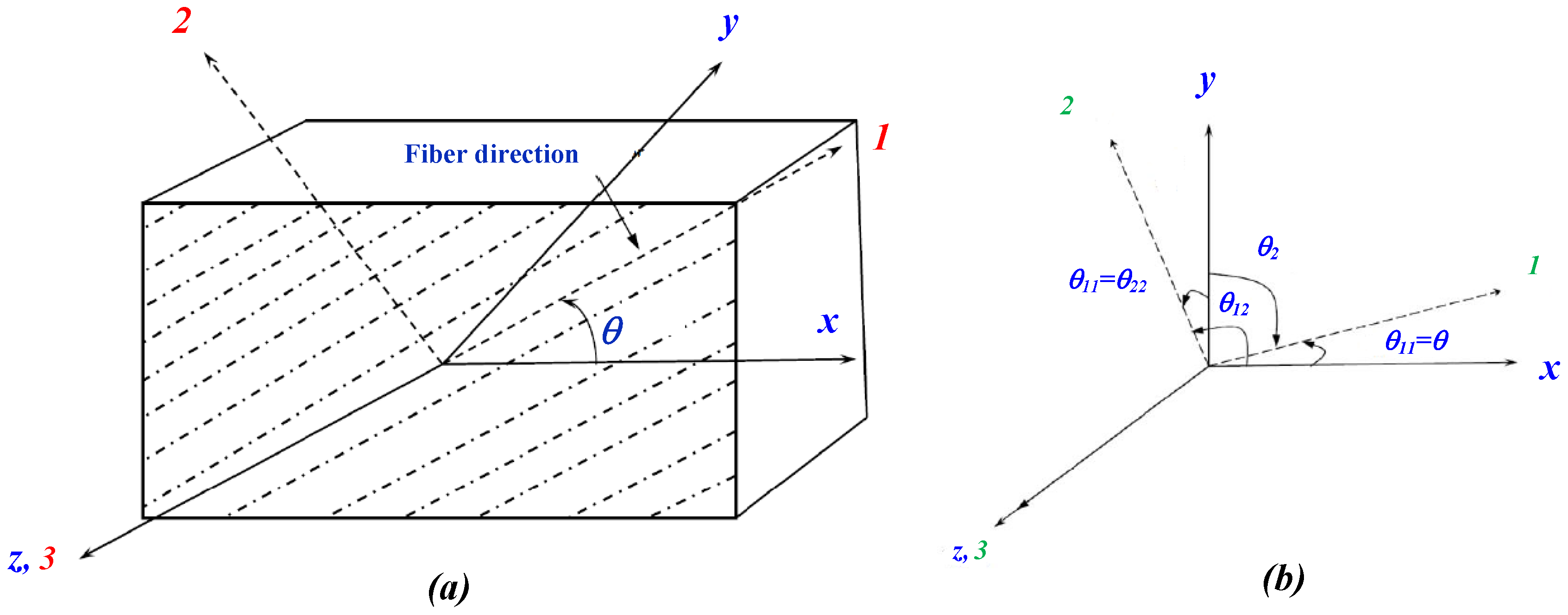
The aforementioned stress–strain relation has been defined in principal material co-ordinate systems ($1,2$, and 3) which are aligned to the fiber direction. However, the global co-ordinates ($x,y$, and z) do not necessarily coincide with the material coordinate system as shown in Figure 1. Thus, it is necessary to represent all the quantities in the global co-ordinates ($x,y$, and z) and the corresponding transformation relationship of stress and strain tensors need to be established. Following Figure 1, if the fiber direction or material co-ordinate axis 1 have the orientation angle $\theta$ with respect to the global co-ordinate axis x in the $x-y$ plane, the second order tensor ${\sigma }_{ij}$ which is defined in material co-ordinate axis can be transformed to stress tensor in global co-ordinate axis, ${\sigma }_{ij}^{\prime }$ as follows [1,3]: ${\sigma }_{ij}^{\prime }=a_{ki}{a}_{lj}{\sigma }_{kl}$. Here, $a_{ik}{a}_{jk}={\delta }_{ij}=1;\forall i=j$ and $a_{ik}{a}_{jk}={\delta }_{ij}=0;\forall i\ne j$. Where, $a_{ij}$ is the directional cosine of the angles measured from the material co-ordinate axis (unprimed axis) $x_i$ to the global co-ordinate axis (primed axis) $x_i^{\prime }$ as shown in Figure 1b. For strain transformation, the engineering shear strain tensor has been utilized which produces the desired symmetric transformed stiffness and compliance tensors.

Transformation about z and y axis: Utilizing the aforementioned stress and strain transformation equations, the relationship between stress in principle material direction, $\left\{\overline{\sigma }\right\}$ and stress in global co-ordinates, ${\left\{\sigma \right\}}_x$ can be obtained as [1,3]: $\left\{\overline{\sigma }\right\}={\left[T_1\right]}_{xy}{\left\{\sigma \right\}}_x$, where ${\left[T_1\right]}_{xy}$ is the stress transformation matrix about rotation in z axis (in $x-y$ plane). Likewise, the strain transformation equation using engineering shear strain is $\left\{\overline{ϵ}\right\}={\left[T_2\right]}_{xy}{\left\{ϵ\right\}}_x$. Similarly, the transformation about y-axis relationship between stresses in principle material direction can be expressed as follows: $\left\{\overline{\sigma }\right\}={\left[T_1\right]}_{xz}{\left\{\sigma \right\}}_x$ and $\left\{\overline{ϵ}\right\}={\left[T_2\right]}_{xz}{\left\{ϵ\right\}}_x$ where, ${\left[T_1\right]}_{xz}$ and ${\left[T_2\right]}_{xz}$ are the stress and strain transformation tensors about rotation in y-axis (in $x-z$ plane), respectively. The expression for the transformed stiffness matrix $\left[\overline{Q}\right]$ in global co-ordinates can be obtained from ${\left\{\sigma \right\}}_x={\left[T_1\right]}^{-1}\left[Q\right]\left[T_2\right]{\left\{ϵ\right\}}_x$ with ${\left[T_i\left(\theta \right)\right]}^{-1}=\left[T_i(-\theta )\right]$$(i=1,2)$ where $\left[\overline{Q}\right]={\left[T_1\right]}^{-1}\left[Q\right]\left[T_2\right]$.

3. Finite Element Formulation

In the present study, finite element (FE) equations have been formulated by employing the energy minimization principle [18]. Considering a control volume v with a body force $\overrightarrow{b}$, traction force vector $\overrightarrow{t}$ with no Neumann boundary condition and homogeneous constraint with displacement vector $\overrightarrow{u}$, one can find $\overrightarrow{u}\in S^0$ such that $\tilde{H}(\overrightarrow{u},\overrightarrow{w})=\tilde{G}(\overrightarrow{w})+\tilde{F}(\overrightarrow{w})\vee \overrightarrow{w}\in S^0$. Here $S^0$ is the space of admissible functions satisfying the Dirichlet boundary conditions; $\overrightarrow{w}$ is the test function; $\tilde{F}(\overrightarrow{w})$ is the virtual work of the applied load; $\tilde{G}(\overrightarrow{w})$ is the virtual work done by the body force, and $\tilde{H}(\overrightarrow{u},\overrightarrow{w})$ is the virtual work of the internal stresses. Thus, the system-energy functional in stable equilibrium can be expressed as [18,19]: $\Pi (\overrightarrow{u})=\tilde{S}(\overrightarrow{u})-\tilde{G}(\overrightarrow{u})-\tilde{F}(\overrightarrow{u})$ where $\tilde{G}(\overrightarrow{u})={\int }_v\overrightarrow{b}.\overrightarrow{u}dv,\tilde{F}(\overrightarrow{u})={\int }_s\overrightarrow{t}.\overrightarrow{u}ds$; $\tilde{S}(\overrightarrow{u})=\frac{1}{2}\tilde{H}(\overrightarrow{u},\overrightarrow{u})=\frac{1}{2}{\int }_v\tilde{\sigma }:\widetilde{ϵ}(\overrightarrow{u})dv$. The solution can be obtained by minimizing the energy functional from the condition ${\delta }^1\Pi (\overrightarrow{u})=\overrightarrow{0}$ which results in

$${\displaystyle {\int }_v\tilde{\sigma }(\overrightarrow{u}):\widetilde{ϵ}(\overrightarrow{w})dv={\int }_v\overrightarrow{b}·\overrightarrow{w}dv+{\int }_s\overrightarrow{t}·\overrightarrow{w}ds.}$$

(1)

In our problem formulation, Equation (1) has been implemented in the FE framework by discretizing the domain into finite number of nodes and elements by using the isoparametric four noded tetrahedron elements. If $n_e$ is the total number of elements, Equation (1) can be discretized as

$${\displaystyle \sum _{e=1}^{n_e}\left[{\int }_{v^e}{\tilde{B}}^T.\tilde{D}.\tilde{B}dv\right]\overrightarrow{u^i}=\sum _{e=1}^{n_e}\left[{\int }_{v^e}{\tilde{N}}^T.\overrightarrow{b}dv+{\int }_{s^e}{\tilde{N}}^T.\overrightarrow{t}ds\right].}$$

(2)

where $\tilde{K}={\displaystyle \sum _{e=1}^{n_e}}\left[{\int }_{v^e}{\tilde{B}}^T.\tilde{D}.\tilde{B}dv\right]$ is the global stiffness matrix, $\overrightarrow{F}={\displaystyle \sum _{e=1}^{n_e}}\left[{\int }_{v^e}{\tilde{N}}^T.\overrightarrow{b}dv+{\int }_{s^e}{\tilde{N}}^T.\overrightarrow{t}ds\right]$ is the external nodal force vector, $\tilde{U}$ is the global nodal displacement vector, $\tilde{N}$ is the shape function matrix, $\tilde{B}$ is the strain-nodal displacement matrix, and $\tilde{D}$ is the elastic tensor. Considering $\overrightarrow{b}=0$, elemental stiffness matrix and external nodal force vector can be expressed from Equations (1) and (2) as follows

$${\displaystyle {\tilde{k}}_e={\int }_{v^e}{\tilde{B}}^T.\tilde{D}.\tilde{B}dv;{\overrightarrow{f}}_e={\int }_{s^e}{\tilde{N}}^T.\overrightarrow{t}ds}$$

(3)

The integrals in Equation (3) can be evaluated by using the Gaussian quadrature integration scheme [18] which requires transformation of three-dimensional subdomain or elements $\tau$ in the physical or global coordinate system $(x,y,z)$ into the subdomains or elements $\widehat{\tau }$ in the local coordinate system $(\xi ,\eta ,\zeta )$. Such transformation can be performed by utilizing the appropriate mapping functions [18,19] as follows

$${\displaystyle {\int }_{v^e}F(x,y,z)dxdydz={\int }_{v^m}F(\xi ,\eta ,\zeta )\left|\mathbf{J}\right|d\xi d\eta d\zeta \simeq \sum _{i=1}^{n_i}w\left(i\right)F({\xi }_i,{\eta }_i,{\zeta }_i)\left|\mathbf{J}\right|}$$

(4)

Here, $v^e$ and $v^m$ are the volume of the physical and master element, respectively; $n_i$ is the total number of integration points; $({\xi }_i,{\eta }_i,{\zeta }_i)$ is the coordinate of integration points and $w\left(i\right)$ is the corresponding weight of integration point. The domain $\Omega$ can be discretized into total elements $\sum {\tau }_i$ which provides the approximate solution over ${\tau }_i$ and corresponding mapping from physical to master co-ordinates yield the element contribution to the global equation for the FE problem. Thus, element stiffness matrix and the force vector in Equation (3) can be obtained by Gauss quadrature method as follows

$${\displaystyle {\tilde{k}}_e={\int }_{v^e}{\tilde{B}}^T.\tilde{D}.\tilde{B}d{v}^e={\int }_{v^m}{\tilde{B}}^T.\tilde{D}.\tilde{B}\left|\mathbf{J}\right|d{v}^m=\sum _{i=1}^{{\tau }_i}w\left(i\right){\tilde{B}}^T.\tilde{D}.\tilde{B}\left|\mathbf{J}\right|}$$

(5)

$${\displaystyle {\overrightarrow{f}}_e={\int }_{s^e}{\tilde{N}}^T.\overrightarrow{t}d{s}^e={\int }_{s^m}{\tilde{N}}^T.\overrightarrow{t}d{s}^m=\sum _{i=1}^{{\tau }_i}w\left(i\right){\tilde{N}}^T.\overrightarrow{t}\left|\mathbf{J}\right|}$$

(6)

After obtaining ${\tilde{k}}_e$ and ${\overrightarrow{f}}_e$, global equations have been solved to the get nodal displacement field for the problem.

Numerical procedure: Due to large degree of unknowns, conjugate gradient based iterative method [20,21] has been utilized to solve the linear system of the form $\mathbf{K}\mathbf{x}=\mathbf{b}$. With $\mathbf{K}$ being symmetric positive definite, the solution is the minimum of the quadratic form which can be defined by paraboloid surface $f\left(x\right)=\frac{1}{2}{\mathbf{x}}^T\mathbf{K}-{\mathbf{b}}^T\mathbf{x}+\mathbf{c}$ with gradient $f^{\prime }\left(x\right)=\frac{1}{2}{\mathbf{K}}^T\mathbf{x}+\frac{1}{2}\mathbf{K}-\mathbf{b}$. In the FE numerical algorithm, an initial point ${\mathbf{x}}_{\left(0\right)}$ on the paraboloid surface has been considered which slides down to a new point which minimizes $f\left(x\right)$. For a new position ${\mathbf{x}}_{\left(i\right)}$, the error can be defined as ${\mathbf{e}}_{\left(i\right)}={\mathbf{x}}_{\left(i\right)}-\mathbf{x}$. With an arbitrary initial point ${\mathbf{x}}_{\left(0\right)}$, the new step can be defined by ${\mathbf{x}}_{(i+1)}={\mathbf{x}}_{\left(i\right)}+{\rho }_{\left(i\right)}{\mathbf{d}}_{\left(i\right)}$, where ${\rho }_{\left(i\right)}$ is the step size in the search direction ${\mathbf{d}}_{\left(i\right)}$. The new ${\mathbf{d}}_{\left(j\right)}$ directions are chosen from the residual vector such a way that it is in orthogonal relationship with the previous residual vectors ${\mathbf{d}}_{\left(i\right)}$ (i.e., ${\mathbf{d}}_{\left(i\right)}^T\mathbf{K}{\mathbf{d}}_{\left(j\right)}=0$) by employing conjugate Gram— Schmidt algorithm [20,21]. The developed FE solver can also be utilized in solving phase transformation equations [22,23,24,25,26,27,28,29,30,31] and other solid mechanics problems [32].

4. Beam Geometry and Material Parameters

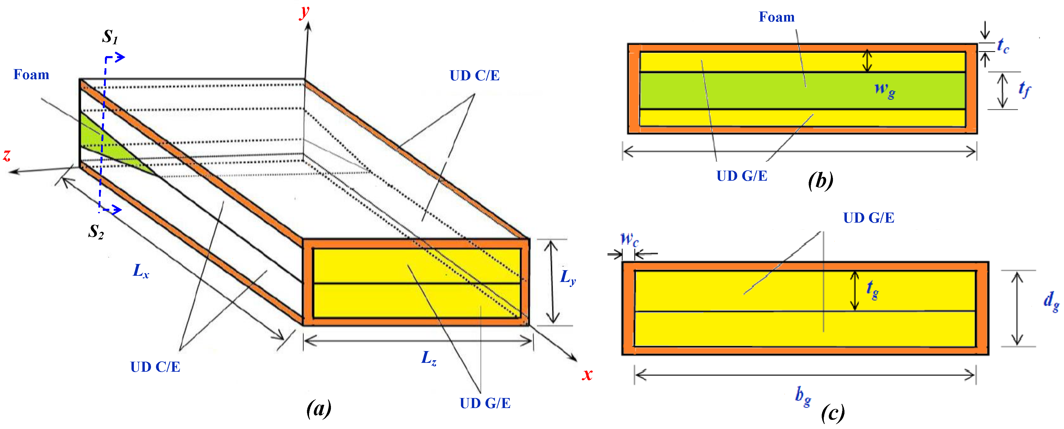
The 3-D beam geometry of the helicopter rotor blade consists of different composite laminates and their arrangements have been shown in Figure 2. The beam of size $L_x\times L_y\times L_z$ is made of three distinct types of composite: unidirectional glass/epoxy (UD G/E), unidirectional ±45° carbon/epoxy (UD C/E), and isotropic foam. The elastic bulk properties of orthotropic UD G/E composite, orthotropic UD C/E composite, and isotropic foam material are collected from [33,34,35,36] and presented in

Table 1. Elastic bulk properties of unidirectional glass/epoxy (UD G/E), unidirectional carbon/epoxy (UD C/E), and isotropic foam for helicopter composite blade [33,34,35,36].

Material	Exx	Eyy	Ezz	Gxy	Gyz	Gzx	νxy	νyz	νzx
	(GPa)	(GPa)	(GPa)	(GPa)	(GPa)	(GPa)
UD G/E [33]	$40.67$	$11.05$	$11.05$	$3.74$	$$3.74$$	$1.052$	$0.378$	$0.277$	$0.277$
UD C/E [34]	$21.10$	$10.05$	$10.05$	$1.87$	$19.60$	$2.95$	$0.343$	$0.581$	$0.182$
Foam [35,36]	$0.07$	$0.07$	$0.07$	-	-	-	$0.251$	$0.251$	$0.251$

. In the FE model, the helicopter blade has been idealized as a cantilever beam which is fixed in the root section, and correspondingly all displacements components are constrained as shown in Figure 2a. In the free end (tip), normal compressive pressure $t_{xx}$, uniform shear traction along y direction $t_{yy}$, and uniform shear traction along z direction $t_{zz}$ have been applied.

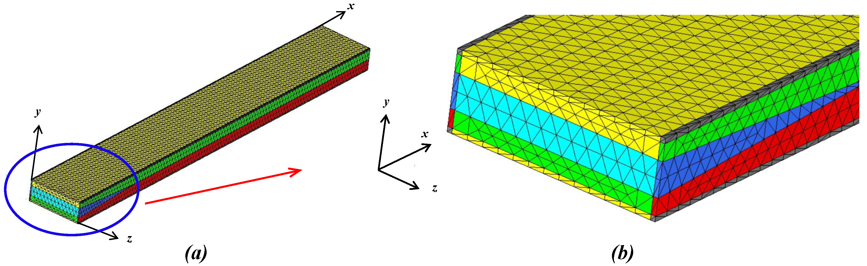
At the free end of the beam (i.e., $x=L_x$), the width of the beam can be expressed as $L_z=2w_c+b_g$, where $w_c$ is the thickness of UD ±45 °C/E laminate along z axis and $b_g$ is the breath of UD G/E as shown in Figure 2c. Whereas, the depth of the beam can be expressed as $L_y=2(t_c+t_g)$. Here, $t_c$ is the thickness of UD ±45 °C/E laminate along y axis and $d_g=2t_g$ is the depth of UD G/E. Such box type UD ±45 °C/E laminate provides the maximum resistance against the external torsional moment as well as axial compressive/tensile load. In the inner core, UD G/E of breath $b_g$ and depth $d_g=2t_g$ provides sufficient stability against bending and axial load. In the root section (i.e., $x=0$), triangular prism-shaped isotropic foam of height $l_f$ along $L_x$ and corresponding foam thickness of $t_f$ at $x=l_f/2$ has been provided for the proper fabrication of the blade. At $x=l_f/2$, width $L_z=2w_c+b_g$ and depth $L_y=2t_c+2w_g+t_f$ can be expressed from the cross section at $S_1-S_2$ as shown in Figure 2b. For our numerical simulation, $t_c+t_g=23$ mm, $w_c+b_g=132$ mm, $l_f=475$ mm, and $L_x=1050$ mm are fixed [6,16] with $t_c^{min}=3$ mm, $w_c^{min}=3$ mm, $t_g^{max}=20$ mm, $b_g^{max}=129$ mm, $t_f^{min}=14$ mm, and $t_f^{max}=21$ mm. Simulation has been performed in the ranges $0.2\le t_c/t_g\le 0.68$ and $0.03\le w_c/b_g\le 0.2$ according to realistic helicopter blade geometric configuration [6,16] for different values of $t_f/L_y$ to determine their influence on tip deformation and stress field behavior in the rotor blade. These parameters can be chosen properly to design an efficient rotor blade system. To achieve a mesh-independent solution, the problem domain $\Omega$ has been approximated by uniformly distributed linear tetrahedral finite elements ${\tau }_i$ of average size 0.27 mm. Furthermore, the mesh independent solution is confirmed by varying the size of the mesh from 0.21 mm to 0.3 mm. HyperMesh [37] has been used to generate mesh for the geometry of the rotor blade which translates the same mesh distribution from one surface to another in the interface between two composite laminates. Additionally, a “mesh masking” technique has been used in order to make the nodal connectivity compatible and coherent at the interface as shown in Figure 3b. In the numerical model, on average, the total number of elements and nodes are considered as 8537 and 24982, respectively, and each simulation takes around 256 core-hours (8 CPU hours) to complete. A user-defined template containing nodal co-ordinates and corresponding connectivity matrix from Hypermesh has been supplemented into in-house Fortran 90 FE code. Utilizing a conjugate gradient solver, the global nodal displacement vector has been obtained. Consequently, complete displacement and stress–strain field have been extracted through in-house Matlab script [38]. In Abaqus FEA model, approximately 8050 total number of C3D8R (linear brick element with reduced integration) elements [39] and 2390 nodes have been considered. The iterative linear equation solver has been implemented utilizing domain decomposition method [39]. For the better convergence of the numerical method, the residual is assigned below a relative tolerance of ${10}^{-6}$. Each simulation takes around 12 CPU hours to complete.

5. Results and Discussions

5.1. Tip Deformations and Stress Fields

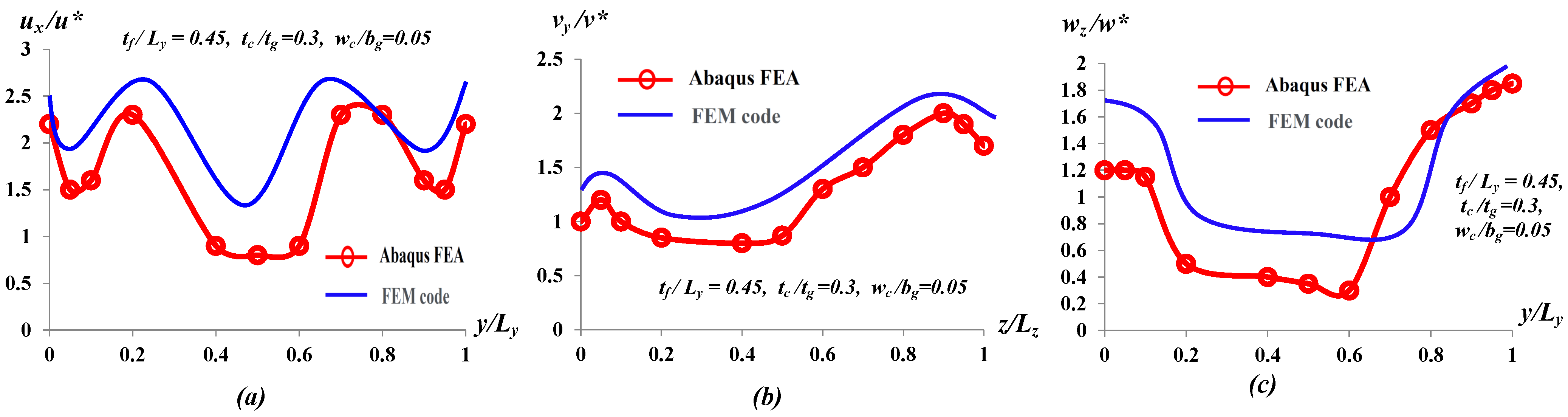
Free end (tip) deformation components and stress fields are the critical design factors in helicopter rotor blade. For the simulation, normal compressive pressure $t_{xx}=100$ MPa, uniform shear traction along y direction $t_{yy}=100$ MPa, and uniform shear traction along z direction $t_{zz}=100$ MPa have been considered at the tip of the rotor. From the FE model, displacement components and stress–strain field at any given cross-section or point of the rotor blade can be obtained. In order to validate the FE framework, numerical results from FE model have been compared with the results from Abaqus FEA [39] for both displacement and stress-field at the tip of the rotor. The distribution of different parts of displacement fields $u_x/u^{*}$ along y at $z=L_z/2$ for applied traction $t_x$, $v_y/v^{*}$ along x at $y=L_y/2$ for applied traction $t_y$, and $w_z/w^{*}$ along y at $z=L_z/2$ for applied traction $t_z$ at the tip of the blade (i.e., $x=L_x$) have been considered and compared between Abaqus FEA and the FE model for specific set of parameters $t_f/L_y=0.45$, $t_c/t_g=0.3$, and $w_c/b_g=0.05$ as shown in Figure 4. Here $u_x$, $v_y$, and $w_z$ are the elemental deformation components and $u^{*}$, $v^{*}$, and $w^{*}$ are the average deformation components [18,19] at the tip cross-sectional area of the rotor along x, y, and z axis, respectively. The distribution of $u_x/u^{*}$ from FE model has the maximum value at the interface of UD C/E and UD G/E laminates (i.e., $y/L_y\simeq 0.24$ and $y/L_y\simeq 0.76$) as shown in Figure 4a. The deformation $u_x/u^{*}$ is relatively high in the UD C/E laminate, whereas the distribution of $u_x/u^{*}$ is relatively low in UD G/E region. This is due to UD G/E laminate has higher stiffness along x -axis compared to UD C/E. Similarly, $w_z/w^{*}$ is significantly high in UD C/E laminate compare to UD C/E and there is a sudden jump in $w_z/w^{*}$ distribution at the interface as shown in Figure 4b. On the other hand, $v_y/v^{*}$ has maximum value at $z/L_z\simeq 0.9$ and it increases monotonically in UD G/E region (i.e., $0.2\le z/L_z\le 0.8$) as shown in Figure 4c. Comparison between Abaqus FEA and FE model indicates good resemblance of displacement fields at the tip of the blade with maximum $\pm 15\%$ deviation. Although, numerical result from FE model reveals that FE model overestimates the Abaqus FEA at the tip of the rotor; however, qualitative distribution of deformation fields are quite similar.

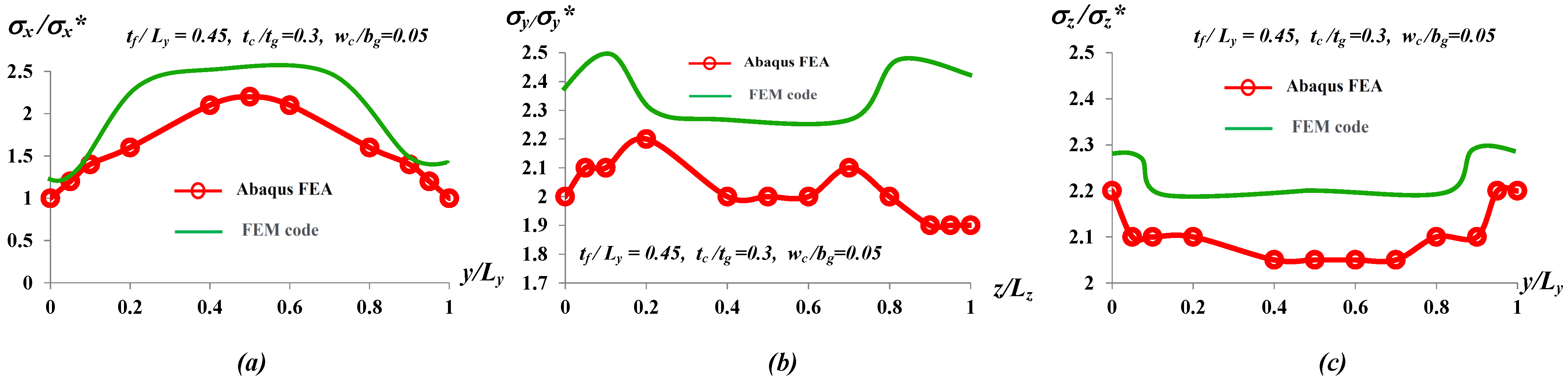
Next, the distribution for different components of stress ${\sigma }_x/{\sigma }^{*}$ along y at $z=L_z/2$ for applied traction $t_x$, ${\sigma }_y/{\sigma }^{*}$ along x at $y=L_y/2$ for applied traction $t_y$, and ${\sigma }_z/{\sigma }^{*}$ along y at $z=L_z/2$ for applied traction $t_z$ at the tip of the blade (i.e., $x=L_x$) for $t_f/L_y=0.45$, $t_c/t_g=0.3$, and $w_c/b_g=0.05$ have been shown in Figure 5. Here, ${\sigma }^{*}$ is the average stress [18,19] at the tip cross-sectional area of the rotor. The numerical result indicates that ${\sigma }_x/{\sigma }^{*}$ is relatively high in UD G/E (i.e., $y/L_y\simeq 0.24$ and $y/L_y\simeq 0.76$) along the depth of the rotor. At the interface between UD C/E and UD G/E, ${\sigma }_x/{\sigma }^{*}$ reduces significantly as shown in Figure 5a. This is because the top and bottom parts of the beam cross-section have UD C/E laminate which is stiffer than UD G/E laminate in loading direction (i.e., along x direction). On the contrary, ${\sigma }_y/{\sigma }^{*}$ in UD C/E is significantly high in UD C/E laminate with the maximum value at the interface (i.e., $y/L_y\simeq 0.2$ and $y/L_y\simeq 0.8$) as shown in Figure 5b. Distribution of ${\sigma }_y/{\sigma }^{*}$ in the UD G/E region is constant. Whereas ${\sigma }_y/{\sigma }^{*}$ decreases along with the depth towards the edge of the cross-section in UD C/E laminate. For ${\sigma }_z/{\sigma }^{*}$ distribution, ${\sigma }_z/{\sigma }^{*}$ has the maximum magnitude in UD C/E region near the edge and the minimum at the midplane in UD C/E region with a jump of ${\sigma }_z/{\sigma }^{*}$ at the interface between these two regions as shown in Figure 5b. The FE numerical results have been compared with Abaqus FEA which indicates good resemblance of ${\sigma }_x/{\sigma }^{*}$ and ${\sigma }_y/{\sigma }^{*}$ distribution with the maximum $\pm 13\%$ deviation from Abaqus FEA result. This deviation can be attributed to the different in discretization parameters and solver configuration between in these two models. However, for ${\sigma }_y/{\sigma }^{*}$, there is significant (almost $\pm 28\%$) deviation at the interface (i.e., $z/L_z\simeq 0.2$ and $z/L_z\simeq 0.8$) between UD C/E and UD G/E laminate. The possible reason for such deviation could be different implication of interface modeling between Abaqus FEA and FE model. Although, FE model results overestimate stress distribution in UD G/E laminate compared to Abaqus FEA; however, the qualitative stress distribution is quite similar for both cases. It is clear from the numerical results and comparisons that the FE model can predict deformation and stress field at the tip of the rotor with reasonable accuracy which validates the correctness of the FE framework.

5.2. Efficient Design of Rotor Blade Geometry

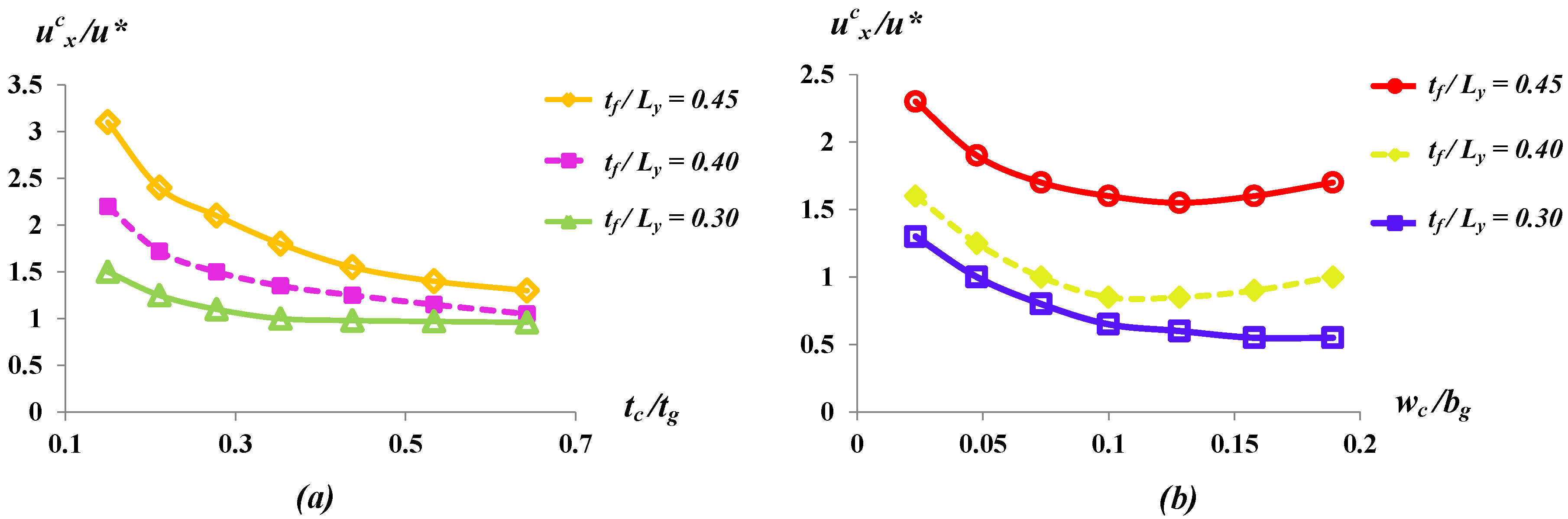
In this section, the effect of $t_c/t_g$ and $w_c/b_g$ which characterizes the overall geometry of the rotor blade on the deformation behavior of the rotor tip has been studied to understand the efficient geometric configurations and arrangements of composite laminates of the rotor blade system. For the study, three different $t_f/L_y=0.45$, $t_f/L_y=0.40$, and $t_f/L_y=0.30$ have been considered which characterize the foam thickness at the fixed end of the composite. For the study, two main dimensionless deformation parameters $u_x^c/u^{*}$ and $v_y^c/v_y^{*}$ have been defined which characterize the overall tip deformation behavior of rotor blade. Here, $u_x^c$ and $v_y^c$ are the deformation components at the centriod of the tip cross section; $u^{*}$ and $v^{*}$ are the average deformation components [18,19] at the tip cross-sectional area of the rotor along x and y axis, respectively.

Dependence of $u_x^c/u^{*}$ on $t_c/t_g$ and $w_c/b_g$: Firstly, the variation of $u_x^c/u^{*}$ as a function of $t_c/t_g$ has been plotted in the range $0.2\le t_c/t_g\le 0.68$ for three different values of $t_f/L_y$ as shown in Figure 6a. In general, increasing $t_c/t_g$ decreases the tip deformation $u_x^c/u^{*}$ for a particular value of $t_f/L_y$. In the range $0.2\le t_c/t_g\le 0.68$, $u_x^c/u^{*}$ is the monotonic decreasing function of $t_c/t_g$ for relatively high $t_f/L_y=0.45$ and $t_f/L_y=0.40$ which suggests that higher $t_c/t_g$ suppress the tip deformation $u_x^c/u^{*}$ for all $t_f/L_y$. The numerical result indicates that, with high $t_c/t_g$, $u_x^c/u^{*}$ converges for different $t_f/L_y$. For relatively low $t_f/L_y=0.45$, $u_x^c/u^{*}$ is independent of $t_c/t_g$ for $t_c/t_g\ge 0.48$. Thus, in order to minimize $u_x^c/u^{*}$, efficient design parameters $t_c/t_g$ and $t_f/L_y$ can be chosen as: $t_c/t_g\le 0.65$ and $0.30\le t_f/L_y\le 0.40$. On the other hand, $u_x^c/u^{*}$ has been plotted as a function of $w_c/b_g$ for different $t_f/L_y$ in order to obtain efficient value of $w_c/b_g$ as shown in Figure 6b. Here, tip deformation $u_x^c/u^{*}$ decrees with increasing $w_c/b_g$ till the threshold value of $w_c/b_g$, ${(w_c/b_g)}^t$ (i.e., slope of $u_x^c/u^{*}$ vs. $w_c/b_g$ equals to 0) for relatively high $t_f/L_y=0.45$ and $t_f/L_y=0.40$. For $w_c/b_g\ge {(w_c/b_g)}^t$, $u_x^c/u^{*}$ increases non-linearly with increasing $w_c/b_g$. Such threshold ${(w_c/b_g)}^t$ depends on $t_f/L_y$. For example, ${(w_c/b_g)}^t\simeq 0.5w_c/b_g$ for $t_f/L_y=0.45$. For relatively low $t_f/L_y=0.40$, the threshold shifts to higher ${(w_c/b_g)}^t\simeq 0.5w_c/b_g$. Clearly, existence of such threshold in $u_x^c/u^{*}$ vs. $w_c/b_g$ corresponds to minima of $u_x^c/u^{*}$ vs. $w_c/b_g$ curve for a particular $t_f/L_y$. Thus, in order to minimize $u_x^c/u^{*}$, efficient design parameters $w_c/b_g$ and $t_f/L_y$ can be chosen as: $w_c/b_g\le 0.12$ and $0.30\le t_f/L_y\le 0.40$.

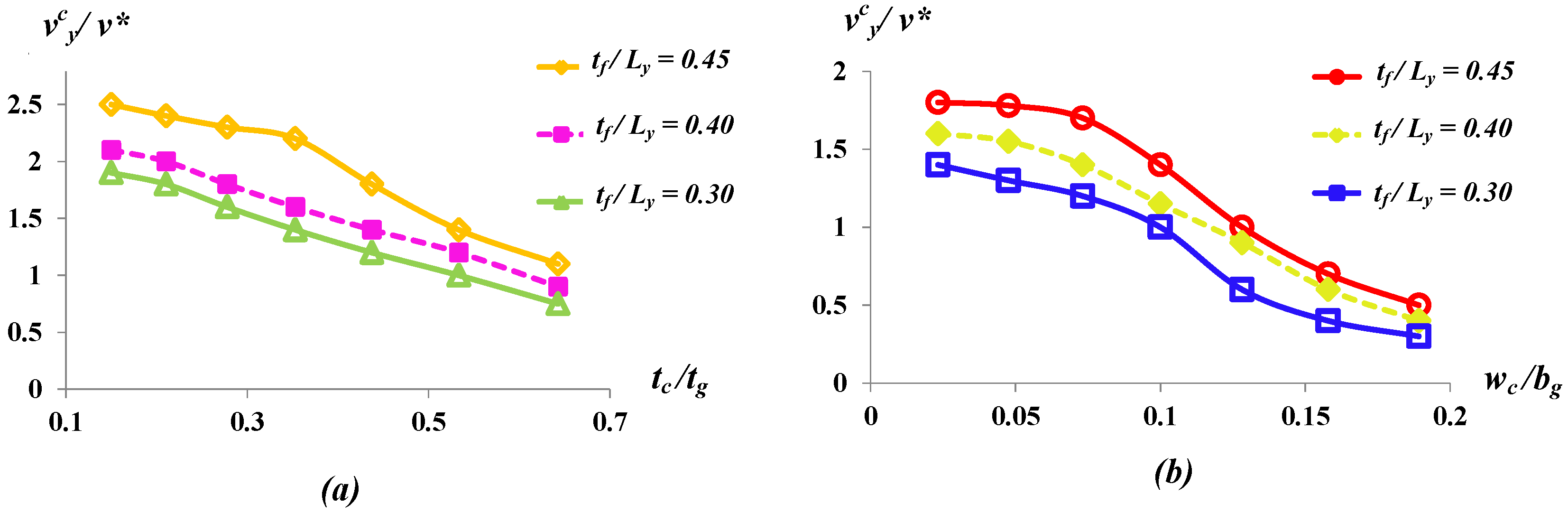
Dependence of $v_y^c/v^{*}$ on $t_c/t_g$ and $w_c/b_g$: Similarly, the variation of $v_x^c/v^{*}$ as a function of $t_c/t_g$ has been plotted in the range $0.2\le t_c/t_g\le 0.68$ for three different values of $t_f/L_y$ as shown in Figure 7a. In general, $v_x^c/v^{*}$ is a decreasing function of $t_c/t_g$ for a particular $t_f/L_y$. However, increasing $t_f/L_y$ increases tip deformation $v_x^c/v^{*}$ for a particular $t_c/t_g$. Our numerical results indicate that $t_f/L_y$ plays an important role to minimize $v_x^c/v^{*}$ for relatively small $t_c/t_g\le 0.45$. However, for relatively high $t_c/t_g\ge 0.55$, the effect of $t_f/L_y$ on $v_x^c/v^{*}$ is not significant. Thus, the efficient design parameter range $0.55\le t_c/t_g\le 0.68$ can be prescribed in order to minimize $v_x^c/v^{*}$ for a particular $t_f/L_y$. Additionally, the dependence of $v_y^c/v^{*}$ on $w_c/b_g$ for different $t_f/L_y$ has been studied in the range $0.03\le w_c/b_g\le 0.2$ as shown in Figure 6b. For a particular $t_f/L_y$, $v_y^c/v^{*}$ decreases with increasing $w_c/b_g$. The numerical result suggests that, with high $w_c/b_g$, deformation parameter $v_y^c/v^{*}$ converges for different $t_f/L_y$. Thus, in order to minimize $v_y^c/v^{*}$, efficient design parameters $w_c/b_g$ and $t_f/L_y$ can be chosen as: $w_c/b_g\ge 0.15$ and $0.30\le t_f/L_y\le 0.40$. From the numerical results, it is clear that higher $t_c/t_g$ minimize $u_x^c/u^{*}$ and $v_x^c/v^{*}$ for a particular $t_f/L_y$. Thus, the ratio $t_c/t_g$ is an important design parameter for the efficient design of helicopter rotor system. On the other hand there is efficient range of $w_c/b_g$ to minimize $u_x^c/u^{*}$ and $v_y^c/v^{*}$. Additionally, $t_f/L_y$ plays an important role to suppress the tip deformation behavior. Hence, it is important to select proper $t_c/t_g$ and $w_c/b_g$ together with $t_f/L_y$ in order to reduce and control deformation characteristic within the desired limit of the rotor blade system. From the analysis, one can effectively design the arrangements of different composite laminates of rotor blade based on optimal $t_c/t_g$ and $w_c/b_g$ values for a given $t_f/L_y$. The current work provides the insights to design the beam geometry efficiently by reducing the overall deflection of the rotor system.

6. Conclusions

Summarizing, a three-dimensional finite element framework has been developed to model full-scale multilaminate composite helicopter rotor blade. The deformation and stress behaviors from the FE model have been studied and compared with Abaqus FEA model for external loading conditions which indicate good resemblance both quantitatively and qualitatively. Furthermore, different geometric design parameters of composite laminates are analyzed to reduce tip deformation and maximize the overall efficiency of the helicopter blade. It is found that these parameters significantly influence tip deformation and can be carefully chosen in order to design an efficient rotor blade system. Present FE framework can be extended to mesoscale damage model for delamination, [40,41,42] hybrid laminated polymer nanocomposite [43,44], and variational asymptotic beam sectional analysis [45,46].

References

- Herakovich, C.T. Mechanics of Fibrous Composites; John Wiley and Sons: New York, NY, USA, 1998. [Google Scholar]
- Chaboche, J.-L. Comprehensive Structural Integrity; Elsevier Pergamon: Amsterdam, The Netherlands; San Diego, CA, USA, 2003. [Google Scholar]
- Barbero, E.J. Introduction to Composite Materials Design; CRC Press: Boca Raton, FL, USA, 2010. [Google Scholar]
- Seddon, J.M.; Simon, N. Basic Helicopter Aerodynamics; John Wiley and Sons: New York, NY, USA, 2011; Volume 40. [Google Scholar]
- Maksimovic, S.; Kozic, M.; Stetic-Kozic, S.; Maksimović, K.; Vasović, I.; Maksimovic, M. Determination of load distributions on main helicopter rotor blades and strength analysis of its structural components. J. Aero. Eng. 2014, 27, 0401–0432. [Google Scholar] [CrossRef]
- Alkahe, J.; Rand, O. Analytic extraction of the elastic coupling mechanisms in composite blades. Compos. Struct. 2000, 49, 399–413. [Google Scholar] [CrossRef]
- Ghiringhelli, G.L.; Masarati, P.; Mantegazza, P. Analysis of an actively twisted rotor by multibody global modeling. Compos. Struct. 2001, 52, 113. [Google Scholar] [CrossRef]
- Morozov, E.V.; Sylantiev, S.A.; Evseev, E.G. Impact damage tolerance of laminated composite helicopter blades. Compos. Struct. 2003, 62, 367–371. [Google Scholar] [CrossRef]
- Conlisk, A.T. Modern helicopter rotor aerodynamics. Prog. Aero. Sci. 2001, 37, 419–476. [Google Scholar] [CrossRef]
- Sirohi, J.; Michael, S.L. Measurement of helicopter rotor blade deformation using digital image correlation. Optic. Eng. 2012, 51, 043603. [Google Scholar] [CrossRef]
- Brocklehurst, A.; Barakos, G.N. A review of helicopter rotor blade tip shapes. Prog. Aero. Sci. 2013, 56, 35–74. [Google Scholar] [CrossRef]
- Kang, H.; Hossein, S.; Gandhi, F. Dynamic blade shape for improved helicopter rotor performance. J. Am. Heli. Soc. 2010, 55, 32008. [Google Scholar] [CrossRef]
- Kumar, A.A.; Viswamurthy, S.R.; Ganguli, R. Correlation of helicopter rotor aeroelastic response with HART-II wind tunnel test data. Air. Eng. Aero. Tech. 2010, 82, 237–248. [Google Scholar] [CrossRef]
- Rasuo, B. Experimental techniques for evaluation of fatigue characteristics of laminated constructions from composite materials: Full-scale testing of the helicopter rotor blades. J. Test. Eval. 2011, 39, 237–242. [Google Scholar]
- Ganguli, R.; Chopra, I.; Haas, D.J. Simulation of helicopter rotor-system structural damage, blade mistracking, friction and freeplay. J. Aircraft 1998, 35, 591. [Google Scholar] [CrossRef]
- Yang, M.; Chopra, I.; Haas, D.J. Sensitivity of rotor-fault-induced vibrations to operational and design parameters. J. Am. Heli. Soc. 2004, 49, 328–339. [Google Scholar] [CrossRef]
- Jones, R.M. Mechanics of Composite Materials, 2nd ed.; CRC Press: Boca Raton, FL, USA, 1999. [Google Scholar]
- Bathe, K.J. Finite Element Procedures; Prentice-Hall: Englewood Cliffs, NJ, USA, 1995. [Google Scholar]
- Lemaitre, J.; Chaboche, J.-L. Mechanics of Solid Materials; Cambridge University Press: Cambridge, UK, 1990; pp. 346–450. [Google Scholar]
- Mansoor, R.; Hosseini, S.M. An ILU preconditioner for nonsymmetric positive definite matrices by using the conjugate Gram-Schmidt process. J. Comp. App. Math. 2006, 188, 150–164. [Google Scholar]
- Straubhaar, J. Preconditioners for the conjugate gradient algorithm using Gram-Schmidt and least squares methods. Int. J. Comp. Math. 2007, 84, 89–108. [Google Scholar] [CrossRef]
- Levitas, V.I.; Roy, A.M.; Preston, D.L. Multiple twinning and variant-variant transformations in martensite: Phase-field approach. Phys. Rev. B 2013, 88, 054113. [Google Scholar] [CrossRef] [Green Version]
- Levitas, V.I.; Roy, A.M. Multiphase phase field theory for temperature-and stress-induced phase transformations. Phys. Rev. B 2015, 91, 174109. [Google Scholar] [CrossRef] [Green Version]
- Levitas, V.I.; Roy, A.M. Multiphase phase field theory for temperature-induced phase transformations: Formulation and application to interfacial phases. Acta Mater. 2016, 105, 244–257. [Google Scholar] [CrossRef] [Green Version]
- Roy, A.M. Multiphase phase field approach for solid-solid phase transformations via propagating interfacial phase in HMX. J. App. Phys. 2021, 129, 025103. [Google Scholar] [CrossRef]
- Roy, A.M. Influence of Interfacial Stress on Microstructural Evolution in NiAl Alloys. JETP Lett. 2020, 112, 173–179. [Google Scholar] [CrossRef]
- Roy, A.M. Effects of interfacial stress in phase field approach for martensitic phase transformation in NiAl shape memory alloys. App. Phys. A 2020, 126, 576. [Google Scholar] [CrossRef]
- Roy, A.M. Evolution of Martensitic Nanostructure in NiAl Alloys: Tip Splitting and Bending. Mat. Sci. Res. Ind. 2020, 17, 3–6. [Google Scholar] [CrossRef]
- Roy, A.M. Barrierless melt nucleation at solid-solid interface in energetic nitramine octahydro-1, 3, 5, 7-tetranitro-1, 3, 5, 7-tetrazocine. Materialia 2021, 15, 101000. [Google Scholar] [CrossRef]
- Roy, A.M. Influence of nanoscale parameters on solid-solid phase transformation in Octogen crystal: Multiple solution and temperature effect. JETP Lett. 2021. [Google Scholar] [CrossRef]
- Roy, A.M. Phase Field Approach for Multiphase Phase Transformations, Twinning, and Variant-Variant Transformations in Martensite. Ph.D. Thesis, Iowa State University, Ames, IA, USA, 2015. [Google Scholar] [CrossRef]
- Solomon, E.; Natarajan, A.; Roy, A.M.; Sundararaghavan, V.; Van der Ven, A.; Marquis, E. Stability and strain-driven evolution of precipitate in Mg-Y alloys. Acta Mater. 2019, 166, 148–157. [Google Scholar] [CrossRef]
- Gusev, A.A.; Peter, J.H.; Ian, M. Fiber packing and elastic properties of a transversely random unidirectional glass/epoxy composite. Compos. Sci. Tech. 2000, 60, 535–541. [Google Scholar] [CrossRef]
- Younes, R.; Hallal, A.; Fardoun, F.; Chehade, F.H. Comparative review study on elastic properties modeling for unidirectional composite materials. Comp. Prop. 2012, 17, 391–408. [Google Scholar]
- Burlayenko, V.N.; Sadowski, T. Effective elastic properties of foam-filled honeycomb cores of sandwich panels. Compos. Struct. 2010, 92, 2890–2900. [Google Scholar] [CrossRef]
- Zhu, H.X.; Knott, J.F.; Mills, N.J. Analysis of the elastic properties of open-cell foams with tetrakaidecahedral cells. J. Mech. Phy. Sol. 1997, 45, 319–343. [Google Scholar] [CrossRef]
- HyperMesh. Available online: www.altair.com/hypermesh (accessed on 1 August 2020).
- MATLAB. Version 7.10.0 (R2010a); The MathWorks Inc.: Natick, MA, USA, 2010. [Google Scholar]
- ABAQUS. Dassault System; Version 6.9; Simulia Corp: Johnston, RI, USA, 2010. [Google Scholar]
- Bruno, D.; Greco, F.; Lonetti, P. A coupled interface-multilayer approach for mixed mode delamination and contact analysis in laminated composites. Int. J. Sol. Struct. 2003, 40, 7245–7268. [Google Scholar] [CrossRef]
- de Borst, R.; Remmers, J.J.C. Computational modeling of delamination. Compos. Sci. Technol. 2006, 66, 713–722. [Google Scholar] [CrossRef]
- Abisset, E.; Daghia, F.; Ladeveze, P. On the validation of a damage mesomodel for laminated composites by means of open-hole tensile tests on quasi-isotropic laminates. Compos. Part A Appl. Sci. Manuf. 2011, 42, 1515–1524. [Google Scholar] [CrossRef]
- Georgantzinos, S.K.; Giannopoulos, G.I.; Markolefas, S.I. Vibration Analysis of Carbon Fiber-Graphene-Reinforced Hybrid Polymer Composites Using Finite Element Techniques. Materials 2020, 13, 4225. [Google Scholar] [CrossRef]
- Georgantzinos, S.K.; Stamoulis, K.P.; Markolefas, S.I. Mechanical Response of Hybrid Laminated Polymer Nanocomposite Structures: A Multilevel Numerical Analysis. SAE Int. J. Aerosp. 2020, 13, 243–256. [Google Scholar] [CrossRef]
- Yu, W.; Hodges, D.H. Elasticity solutions versus asymptotic sectional analysis of homogeneous, isotropic, prismatic beams. J. App. Mech. 2004, 71, 15–23. [Google Scholar] [CrossRef]
- Yu, W.; Hodges, D.H.; Ho, J.C. Variational asymptotic beam sectional analysis—An updated version. Int. J. Eng. Sci. 2012, 59, 40–64. [Google Scholar] [CrossRef]
Figure 1.
(a) Schematic of a unidirectional orthotrophic composite laminate with principal material co-ordinate system (, and 3) and global co-ordinates (, and z). (b) Principal material axis 3 is rotated by in plane with anticlockwise angle with respect to x-axis is taken as positive.
Figure 2.
(a) 3-D beam geometry of the helicopter rotor blade consisting of unidirectional glass/epoxy (UD G/E), unidirectional ±45° carbon/epoxy (UD C/E), and isotropic foam; (b) cross section near the root; (c) cross section at the tip of the rotor.
Figure 3.
(a) Typical finite element mesh with liner tetrahedral elements in Hypermesh [37]; (b) zoomed part of the root showing the nodal continuity of different parts of composite laminate in the finite element (FE) model.
Figure 4.
Distribution and comparison of different parts of displacement field between Abaqus FEA and FE model for (a) along y at for applied traction ; (b) along x at for applied traction ; (c) along y at for applied traction at the tip of the blade (i.e., ) for , , and .
Figure 5.
Distribution and comparison of different parts of stress fields between the numerical results of Abaqus FEA and FE model for (a) along y at for applied traction ; (b) along x at for applied traction ; (c) along y at for applied traction MPa at the tip of the blade(i.e., ) for , , and .
Figure 6.
Variation of as a function of (a) in the range and (b) in the range for different values of .
Figure 7.
Publisher’s Note: MDPI stays neutral with regard to jurisdictional claims in published maps and institutional affiliations. |
© 2021 by the author. Licensee MDPI, Basel, Switzerland. This article is an open access article distributed under the terms and conditions of the Creative Commons Attribution (CC BY) license (http://creativecommons.org/licenses/by/4.0/).
Share and Cite
MDPI and ACS Style
Roy, A.M. Finite Element Framework for Efficient Design of Three Dimensional Multicomponent Composite Helicopter Rotor Blade System. Eng 2021, 2, 69-79. https://0-doi-org.brum.beds.ac.uk/10.3390/eng2010006
AMA Style
Roy AM. Finite Element Framework for Efficient Design of Three Dimensional Multicomponent Composite Helicopter Rotor Blade System. Eng. 2021; 2(1):69-79. https://0-doi-org.brum.beds.ac.uk/10.3390/eng2010006
Chicago/Turabian StyleRoy, Arunabha M. 2021. "Finite Element Framework for Efficient Design of Three Dimensional Multicomponent Composite Helicopter Rotor Blade System" Eng 2, no. 1: 69-79. https://0-doi-org.brum.beds.ac.uk/10.3390/eng2010006