An Iterative Hybrid Algorithm for Roots of Non-Linear Equations

Abstract

Finding the roots of non-linear and transcendental equations is an important problem in engineering sciences. In general, such problems do not have an analytic solution; the researchers resort to numerical techniques for exploring. We design and implement a three-way hybrid algorithm that is a blend of the Newton–Raphson algorithm and a two-way blended algorithm (blend of two methods, Bisection and False Position). The hybrid algorithm is a new single pass iterative approach. The method takes advantage of the best in three algorithms in each iteration to estimate an approximate value closer to the root. We show that the new algorithm outperforms the Bisection, Regula Falsi, Newton–Raphson, quadrature based, undetermined coefficients based, and decomposition-based algorithms. The new hybrid root finding algorithm is guaranteed to converge. The experimental results and empirical evidence show that the complexity of the hybrid algorithm is far less than that of other algorithms. Several functions cited in the literature are used as benchmarks to compare and confirm the simplicity, efficiency, and performance of the proposed method.

1. Introduction

The construction of numerical solutions for non-linear equations is essential in many branches of science and engineering. Most of the time, non-linear problems do not have analytic solutions; the researchers resort to numerical methods. New efficient methods for solving nonlinear equations are evolving frequently, and are ubiquitously explored and exploited in applications. Their purpose is to improve the existing methods, such as classical Bisection, False Position, Newton–Raphson, and their variant methods for efficiency, simplicity, and approximation reliability in the solution.

There are various ways to approach a problem; some methods are based on only continuous functions while others take advantage of the differentiability of functions. The algorithms such as Bisection using midpoint, False Position using secant line intersection, and Newton–Raphson using tangent line intersection are ubiquitous. There are improvements of these algorithms for speedup; more elegant and efficient implementations are emerging. The variations of continuity-based Bisection and False Position methods are due to Dekker [1,2], Brent [3], Press [4], and several variants of False Position including the reverse quadratic interpolation (RQI) method. The variations of derivative based quadratic order Newton–Raphson method are 3rd, 4th, 5th, 6th order methods. From these algorithms, the researcher has to find a suitable algorithm that works best for every function [5,6]. For example, the bisection method for a simple equation x − 2 = 0, on interval [0, 4], will get the solution in one iteration. However, if the same algorithm is used on a different, smaller interval [0, 3], iterations will go on forever to get to 2; it will need some tolerance on error or on the number of iterations to terminate the algorithm.

For derivative based methods, several predictor–corrector solutions have been proposed for extending the Newton–Raphson method with the support of Midpoint (mean of endpoints of domain interval), Trapezoidal (mean of the function values at the endpoint of the domain), Simpsons (quadratic approximation of the function) quadrature formula [7], undetermined coefficients [8], a third order Newton-type method to solve a system of nonlinear equations [9], Newton’s method with accelerated convergence [10] using trapezoidal quadrature, fourth order method of undetermined coefficients [11], one derivative and two function evaluations [12], Newton’s Method using fifth order quadrature formulas [13], using Midpoint, Trapezoidal, and Simpson quadrature sixth order rule [14]. Newton–Raphson and its variants use the derivative of the function; the derivative of the function is computed from integrations using quadrature-based methods. The new three-way hybrid algorithm presented here does not use any variations or quadrature or method of undetermined coefficient, and still, it competes with all these algorithms.

For these reasons, a two-way blended algorithm was designed and implemented that is a blend of the bisection algorithm and regula falsi algorithm. It does not take advantage of the differentiability of the function [15]. Most of the time, the equations involve differentiable functions. To take advantage of differentiability, we design a three-way hybrid algorithm that is a hybrid of three algorithms: Bisection, False Position, and Newton–Raphson. The hybrid algorithm is a new single pass iterative approach. The method does not use predictor–corrector technique, but predicts a better estimate in each iteration. The new algorithm is promising in outperforming the False Position algorithm and the Newton–Raphson algorithm. Table 1 is a listing of all the methods used for test cases. It is also confirmed [Table 2, Table 3, Table 4 and Table 5] that it outperforms the quadrature based [7,13,14], undetermined coefficients methods [8], and decomposition based [16] algorithms in terms of number of function evaluations per iteration as well as overall number of iterations, computational order of convergence (COC), and efficiency index (EFF). This hybrid root finding algorithm performs fewer or at most that many iterations as these cited methods or functions. The bisection and regula falsi algorithms require only continuity and no derivatives. This algorithm is guaranteed to converge to a root. The hybrid algorithm utilizes the best of the three techniques. The theoretical and empirical evidence shows that the computational complexity of the hybrid algorithm is considerably less than that of the classical algorithms. Several functions cited in the literature are used to confirm the simplicity, efficiency, and performance of the proposed method. The resulting iteration counts are compared with the existing iterative methods in Table 2.

Even though the classical methods have been developed and used for decades, enhancements are made to improve the performance of these methods. A method may perform better than other methods on one dataset, and may produce inferior results on another dataset. We have seen an example just above that different methods have their own strengths/weaknesses. A dynamic new hybrid algorithm is presented here by taking advantage of the best in the Bisection, False Position, and Newton–Raphson methods to locate the roots independent of Dekker, Brent, RQI, and 3rd–6th order methods. Its computational efficiency is validated by comparing it with the existing methods via complexity analysis and empirical evidence. This new hybrid algorithm outperforms all the existing algorithms; see Section 4 for empirical outcomes validating the performance of the new algorithm.

This paper is organized as follows. Section 2 describes background methods to support the new algorithm. Section 3 is the new algorithm. Section 4 is experimental analysis using a multitude of examples used by researchers in the literature, results, and comparison with their findings. Section 5 is on the complexity of computations. Section 6 is the conclusion followed by references.

2. Background, Definitions

In order to review the literature, we briefly describe methods for (1) root approximation, (2) error calculation and error tolerance, and (3) algorithm termination criteria. There is no single optimal algorithm for root approximation. Normally we look for the solution in the worst-case scenario. The order of complexity does not tell the complete detailed outcome. The computational outcome may depend on implementation details, the domain, tolerance, and the function. No matter what, for comparison with different algorithms accomplishing the same task, we use the same function, same tolerance, same termination criteria to justify the superiority of one algorithm over the other. When we are faced with competing choices, normally the simplest one is the accurate one. This is particularly true in this case. We provide a new algorithm that is simpler and outperforms all these methods. For background, we will briefly refer to two types of equations: (1) those requiring only continuous functions, and (2) those requiring differentiable functions along with the desired order of derivative in their formulations.

There are two types of problems: (1) continuity based with no derivative requirement, such as Bisection, False Position, and their extensions; and (2) derivative based, such as Newton–Raphson and its variations. For simulations, we use error Tolerance $\epsilon$ = 0.0000001, tolerance coupled with iterations termination criteria as (|x_k $-$ x_k−1| + |f(x_k)|) < $\epsilon$, and upper bound on iterations as 100: for function f:[a, b] → R, such that

(1) f(x) is continuous on the interval [a, b], where R is the set of all real numbers, and

(2) f(a) and f(b) are of opposite signs, i.e., f(a)·f(b) < 0, then there exists a root r ∈ [a, b] such that f(r) = 0, or

(2′) the function f(x) is differentiable with g(x) = x − f(x)/f′(x) and |g′(x) < 1, then there exists a root r ∈ [a, b] such that f(r) = 0.

Since the solution is obtained by iterative methods, the definition of convergence is as follows:

Definition (Convergence)

[10,12,17]. Let x_n, and $\alpha$ ∈ R, n ≥ 0. Then, the sequence {x_n} is said to converge to $\alpha$ if

$$\underset{n\to \infty }{\lim }|{\mathrm{x}}_{\mathrm{n}}-\alpha |=1$$

Definition (Order of Convergence).

Let x_n, and $\alpha$ ∈ R, n ≥ 0, sequence {x_n} converge to $\alpha$.

In addition, [12,18] if there exists a constant C > 0 (C ≠ 0, C ≠$\infty$) and an integer p ≥ 1 such that

$$\underset{n\to \infty }{\lim }\left(\frac{\left|x_{n+1}-\alpha \right|}{{\left|x_n-\alpha \right|}^p}\right)=\mathrm{C}$$

then the sequence {x_n} is said to converge to $\alpha$ with convergence order p, and C is the asymptotic error constant [10,12,18,19].

Since x_n = $\alpha$ + e_n, the error equation becomes

e_n+1 = C e_n^p + O(e_n^p+1)

If p = 1, 2, or 3, the convergence is called linear, quadratic, or cubic convergence, respectively.

These theoretical criteria do not take into consideration how much computation the function values perform in each step. The order of convergence p can be approximated by the Computational Order of Convergence (COC) that takes into account the combinatorial cost of the method.

Definition (Computational Order of Convergence).

Suppose three iterations$x_{n-1}$, $x_n$, $x_{n+1}$are closer to the root$\alpha$; then, the order of convergence is approximated by [10,12,14]

$$\mathrm{COC}=\underset{n\to \infty }{\lim }\left(\frac{\log |\frac{|{\mathrm{x}}_{\mathrm{n}+1}-\mathsf{\alpha }|}{|{\mathrm{x}}_{\mathrm{n}}-\mathsf{\alpha }|}|}{\log |\frac{|{\mathrm{x}}_{\mathrm{n}}-\mathsf{\alpha }|}{|{\mathrm{x}}_{\mathrm{n}-1}-\mathsf{\alpha }|}|}\right)$$

Additionally, since$\alpha$is not known a priori, there are other ways to compute COC, namely, using four iterations [8] instead of three iterations [10,12,17].

$$\mathrm{COC}=\underset{n\to \infty }{\lim }\left(\frac{\log |\frac{|{\mathrm{x}}_{\mathrm{n}+1}-{\mathrm{x}}_{\mathrm{n}}|}{|{\mathrm{x}}_{\mathrm{n}}-{\mathrm{x}}_{\mathrm{n}-1}|}|}{\log |\frac{|{\mathrm{x}}_{\mathrm{n}}-{\mathrm{x}}_{\mathrm{n}-1}|}{|{\mathrm{x}}_{\mathrm{n}-1}-{\mathrm{x}}_{\mathrm{n}-2}|}|}\right)$$

Definition (Efficiency Index).

If the power p is the order of convergence and q is the number of function evaluations per iteration, then p^1/q is called the efficiency index and is denoted by EFF [10,12].

2.1. Bisection Method

The Bisection method (1) is a binary approach for eliminating subintervals, (2) is virtually a binary search, and (3) converges slowly to the root. Without regard to the function, an upper bound on the root error is fixed at each iteration and it can be computed a priori. By specifying the tolerance on root error, the upper bound on the number of iterations is predetermined.

2.2. False Position (Regula Falsi) Method

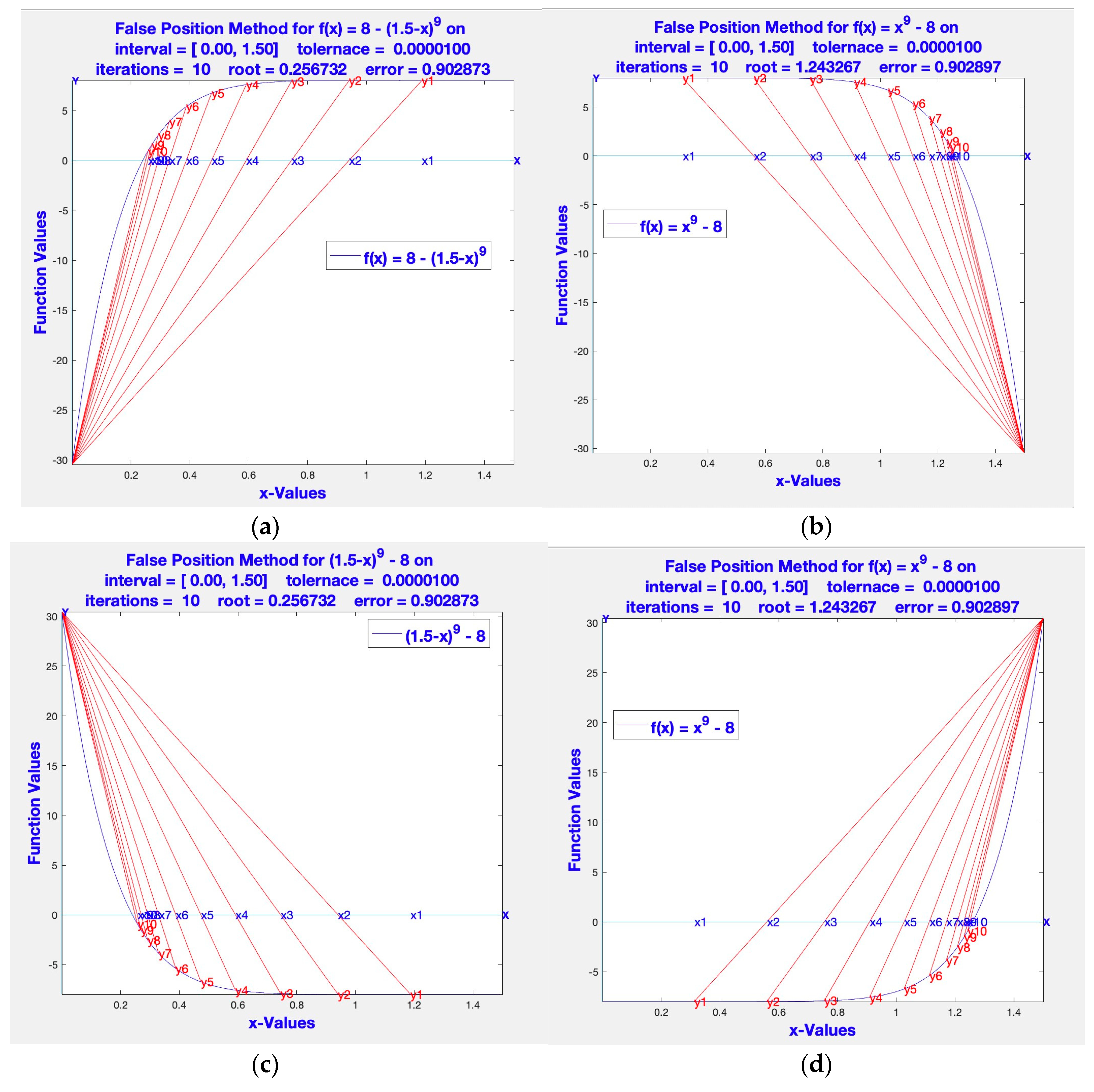
The poor performance of the Bisection method led to the False Position method. It finds zeros of the function by linear interpolation. The False Position uses the location of the root for better selection. Unfortunately, this method does not perform as well as expected for all functions; see Figure 1 [15] for four types of concavity in the function. Iterations are terminated at ten to keep the plots clean. The figures show that the False Position method performs poorly as compared to the Bisection method.

2.3. Dekker’s Method

Dekker algorithm [2] was designed to circumvent the shortcomings of the slow speed of the Bisection and the uncontrolled iteration count of the False Position method. It is a combination of two methods: Bisection and False Position. First of all, it assumes that f(x) is continuous on [a, b] and f(a)f(b) < 0. It maintains that |f(b)| < |f(a)|; otherwise, a and b are exchanged to ensure that b is the “best” estimate of the approximate root. The algorithm maintains that {b_k} is the sequence of best estimates, and the root enclosing interval is always [a_k, b_k] or [b_k, a_k]. Dekker’s algorithm maintain three values: b is the current best approximation, c is the previous approximation b_k−1, and a is the contrapoint so that the root lies in the interval [a_k, b_k]${\displaystyle \cup }$[b_k, a_k]. Both the secant point, s, and midpoint, m, are computed; b_k is s or m, whichever is closest to b_k−1. Though it is better than the False position method, nonetheless, it has some road blocks, handled by Brent.

2.4. Brent’s Algorithm

Brent’s algorithm [3] evolved from the failures of Dekker’s algorithm; it is a step towards the improvement of Dekker’s algorithm. It is a slight improvement at the cost of extra test computations. It is a combination of four methods, Bisection, False Position, Dekker, and reverse (a.k.a. inverse) quadratic interpolation (RQI), described next. Reverse quadratic interpolation is based on the method of Lagrange polynomials and it leads to extra calculations. Thus, it may take more iterations to circumvent pathological cases. It uses three estimates to derive the next estimate. This algorithm is more robust and more costly.

Detour to Reverse Quadratic Interpolation

Let a, b, and c be three distinct points, and f(a), f(b), and f(c) be corresponding distinct values of the function f(x); there is a unique quadratic polynomial through three points (a, f(a)), (b, f(b)), (c, f(c)). The Lagrange form of polynomial is most suitable for evaluation of the polynomial for values of x and inverse value of y. In fact, there is a direct formula for a reverse quadratic interpolating (RPI) polynomial that can be evaluated from values of y.

$$\mathrm{x}=\frac{(\mathrm{y}-\mathrm{f}(\mathrm{b}))(\mathrm{y}-\mathrm{f}(\mathrm{c}))}{(\mathrm{f}(\mathrm{a})-\mathrm{f}(\mathrm{b}))(\mathrm{f}(\mathrm{a})-\mathrm{f}(\mathrm{c}))}\mathrm{a}+ \frac{(\mathrm{y}-\mathrm{f}(\mathrm{a}))(\mathrm{y}-\mathrm{f}(\mathrm{c}))}{(\mathrm{f}(\mathrm{b})-\mathrm{f}(\mathrm{a}))(\mathrm{f}(\mathrm{b})-\mathrm{f}(\mathrm{c}))}\mathrm{b}+\frac{(\mathrm{y}-\mathrm{f}(\mathrm{a}))(\mathrm{y}-\mathrm{f}(\mathrm{b}))}{(\mathrm{f}(\mathrm{c})-\mathrm{f}(\mathrm{a}))(\mathrm{f}(\mathrm{c})-\mathrm{f}(\mathrm{b}))}\mathrm{c}$$

or

$${\mathrm{x}}_{\mathrm{k}+1}=\frac{\mathrm{af}(\mathrm{b})\mathrm{f}(\mathrm{c})}{(\mathrm{f}(\mathrm{a})-\mathrm{f}(\mathrm{b}))(\mathrm{f}(\mathrm{a})-\mathrm{f}(\mathrm{c}))}+\frac{\mathrm{bf}(\mathrm{c})\mathrm{f}(\mathrm{a})}{(\mathrm{f}(\mathrm{b})-\mathrm{f}(\mathrm{c}))(\mathrm{f}(\mathrm{b})-\mathrm{f}(\mathrm{a}))}+\frac{\mathrm{cf}(\mathrm{a})\mathrm{f}(\mathrm{b})}{(\mathrm{f}(\mathrm{c})-\mathrm{f}(\mathrm{a}))(\mathrm{f}(\mathrm{c})-\mathrm{f}(\mathrm{b}))}$$

The derivative based methods depend on the initial start point, x₀. The simplest such technique is the Newton–Raphson method, which is slower than its variations. These algorithms outperform the conventional Newton–Raphson method. The variations include decomposition based [16], quadrature based, and undetermined coefficients based [11,13,14]. These methods are quite complex and detailed. The reader may wish to refer to the full papers for details. For completeness, we describe the iteration formulas to show how these methods iterate to get to the root.

2.5. Newton-Raphson (1760)

Let f be differentiable on an open interval containing a, b. By Taylor series expansion of f,

$$\mathrm{f}(\mathrm{b})=\mathrm{f}(\mathrm{a})+(\mathrm{b}-\mathrm{a})\mathrm{f}{}^{\prime }(\mathrm{a})+\frac{1}{2!}(\mathrm{b}-\mathrm{a}{)}^2\mathrm{f}{}^{″}(\mathrm{a})+\dots +$$

By retaining the first derivative term only, linear approximation of order one

$$\mathrm{f}(\mathrm{b})\cong \mathrm{f}(\mathrm{a})+(\mathrm{b}-\mathrm{a}){\mathrm{f}}^{\prime }(\mathrm{a})$$

Assuming the value of b to be close to the root of f, further leads to

$$0\cong \mathrm{f}(\mathrm{a})+(\mathrm{b}-\mathrm{a}){\mathrm{f}}^{\prime }(\mathrm{a})$$

b = $\mathrm{a}-\frac{\mathrm{f}(\mathrm{a})}{\mathrm{f}{}^{\prime }(\mathrm{a})}$ which is standard Newton–Raphson method.

Thus, for function f, Newton–Raphson [17] successive estimates for the solution are

$$x_{n+1}= x_n-\frac{f(x_n)}{f^{\prime }(x_n)}$$

(1)

with quadratic order of error, O($ϵ$²), where $ϵ$= |$x_{n+1}-x_n$|.

This amounts to two function evaluations for each iteration. However, if we write

$$\mathrm{g}({\mathrm{x}}_{\mathrm{n}})={\mathrm{x}}_{\mathrm{n}}-\frac{\mathrm{f}({\mathrm{x}}_{\mathrm{n}})}{\mathrm{f}{}^{\prime }({\mathrm{x}}_{\mathrm{n}})}$$

then

$${\mathrm{x}}_{\mathrm{n}+1}=\mathrm{g}({\mathrm{x}}_{\mathrm{n}})$$

amounts to one function evaluation for each iteration. It is just a matter of how we count the number of function evaluations. It is of theoretical interest, but really, we have to consider the combinatorial cost of the function, too. In fact, we can write

$${\mathrm{x}}_{\mathrm{n}+1}={\mathrm{x}}_{\mathrm{n}}-\frac{\mathrm{f}({\mathrm{x}}_{\mathrm{n}})({\mathrm{x}}_{\mathrm{n}}-{\mathrm{x}}_{\mathrm{n}-1})}{(\mathrm{f}({\mathrm{x}}_{\mathrm{n}})-\mathrm{f}({\mathrm{x}}_{\mathrm{n}-1}))}$$

That results in one function evaluation $\mathrm{f}({\mathrm{x}}_{\mathrm{n}})$ in every iteration. We use this form in the algorithm.

2.6. Oghovese-John Method (2014)

The Oghovese–John sixth order method approximates the iteration estimates by using the average of Midpoint and Simpson quadrature, and it is shown to have approximation accuracy of order six.

The expression for Oghovese–John’s estimates [7] is as follows.

Let

$$\begin{gathered} {\mathrm{u}}_0={\mathrm{x}}_0-\frac{\mathrm{f}({\mathrm{x}}_0)}{\mathrm{f}{}^{\prime }({\mathrm{x}}_0)} \\ {\mathrm{v}}_0={\mathrm{u}}_0-\frac{\mathrm{f}({\mathrm{u}}_0)}{\mathrm{f}{}^{\prime }({\mathrm{u}}_0)} \end{gathered}$$

Then, for n ≥ 0

$${\mathrm{u}}_{\mathrm{n}+1}={\mathrm{u}}_{\mathrm{n}}-\frac{\mathrm{f}({\mathrm{u}}_{\mathrm{n}})}{\mathrm{f}{}^{\prime }({\mathrm{u}}_{\mathrm{n}})}$$

(2)

$${\mathrm{v}}_{\mathrm{n}+1}={\mathrm{v}}_{\mathrm{n}}-\frac{12\mathrm{f}({\mathrm{v}}_{\mathrm{n}})}{\mathrm{f}{}^{\prime }(({\mathrm{v}}_{\mathrm{n}})+10\mathrm{f}{}^{\prime }(\frac{({\mathrm{v}}_{\mathrm{n}}+{\mathrm{u}}_{\mathrm{n}+1}}{2})+\mathrm{f}{}^{\prime }({\mathrm{u}}_{\mathrm{n}+1})}$$

(3)

(Based on the average of Midpoint and Simpsons 3/8 rule.)

Then, the iterates, x_n+1, are defined in terms of ${\mathrm{v}}_{\mathrm{n}}$ instead of ${\mathrm{x}}_{\mathrm{n}}$

$${\mathrm{x}}_{\mathrm{n}+1}={\mathrm{v}}_{\mathrm{n}}-\frac{\mathrm{f}({\mathrm{v}}_{\mathrm{n}})}{\mathrm{f}{}^{\prime }({\mathrm{v}}_{\mathrm{n}})}\mathrm{for}\mathrm{n}\ge 0$$

(4)

instead of Newton–Raphson formula x_n+1 =${\mathrm{x}}_{\mathrm{n}}–\frac{\mathrm{f}({\mathrm{x}}_{\mathrm{n}})}{\mathrm{f}{}^{\prime }({\mathrm{x}}_{\mathrm{n}})}$

Convergence and stopping criteria are specified with error tolerance and upper bound on iterations for termination. In fact, the algorithm terminates considerably much earlier than it reaches any termination condition in the algorithm.

The derivation of the Oghovese–Emunefe [7] method uses the average of Midpoint and Simpson quadrature. We briefly describe its derivation in Appendix A.

The following variations are very interesting and challenging. It is a historical perspective [18,19,20,21,22,23,24] of development of innovations in the improvement of the Newton–Raphson method and its variants for solution to non-linear equations. We will compare the hybrid algorithm with these. First, we describe their iteration recurrence relations without derivations and defer their derivations to references for simplicity.

2.7. Grau-Diaz-Barero (2006)

Grau et al. [18] introduced a new method by correcting Ostrowski’s method [12]:

$${\mathrm{y}}_{\mathrm{n}}={\mathrm{x}}_{\mathrm{n}}-\frac{\mathrm{f}({\mathrm{x}}_{\mathrm{n}})}{\mathrm{f}{}^{\prime }({\mathrm{x}}_{\mathrm{n}})}$$

(5)

$${\mathrm{x}}_{\mathrm{n}+1}={\mathrm{y}}_{\mathrm{n}}-\frac{\mathrm{f}({\mathrm{y}}_{\mathrm{n}})}{\mathrm{f}{}^{\prime }({\mathrm{x}}_{\mathrm{n}})}\frac{2\mathrm{f}({\mathrm{x}}_{\mathrm{n}})-f({\mathrm{y}}_{\mathrm{n}})}{2\mathrm{f}({\mathrm{x}}_{\mathrm{n}})-5\mathrm{f}({\mathrm{y}}_{\mathrm{n}})}$$

(6)

The method uses one derivative and two function evaluations.

The method has a sixth order convergence with the following iterations:

$${\mathrm{y}}_{\mathrm{n}}={\mathrm{x}}_{\mathrm{n}}-\frac{\mathrm{f}({\mathrm{x}}_{\mathrm{n}})}{\mathrm{f}{}^{\prime }({\mathrm{x}}_{\mathrm{n}})}$$

(7)

$${\mathrm{z}}_{\mathrm{n}}={\mathrm{y}}_{\mathrm{n}}-\frac{\mathrm{f}({\mathrm{y}}_{\mathrm{n}})}{\mathrm{f}{}^{\prime }({\mathrm{x}}_{\mathrm{n}})}\frac{\mathrm{f}({\mathrm{x}}_{\mathrm{n}})}{\mathrm{f}({\mathrm{x}}_{\mathrm{n}})-2\mathrm{f}({\mathrm{y}}_{\mathrm{n}})}$$

(8)

$${\mathrm{x}}_{\mathrm{n}+1}={\mathrm{z}}_{\mathrm{n}}-\frac{\mathrm{f}({\mathrm{z}}_{\mathrm{n}})}{\mathrm{f}{}^{\prime }({\mathrm{x}}_{\mathrm{n}})}\frac{\mathrm{f}({\mathrm{x}}_{\mathrm{n}})}{\mathrm{f}({\mathrm{x}}_{\mathrm{n}})-2\mathrm{f}({\mathrm{y}}_{\mathrm{n}})}$$

(9)

2.8. Sharma-Guha (2007)

Sharma and Guha [22] modified and parameterized Ostrowski’s method [12] having four function evaluations and a sixth order convergence. Their formula is given as follows:

$${\mathrm{y}}_{\mathrm{n}}={\mathrm{x}}_{\mathrm{n}}-\frac{\mathrm{f}({\mathrm{x}}_{\mathrm{n}})}{\mathrm{f}{}^{\prime }({\mathrm{x}}_{\mathrm{n}})}$$

(10)

$${\mathrm{z}}_{\mathrm{n}}={\mathrm{y}}_{\mathrm{n}}-\frac{\mathrm{f}({\mathrm{y}}_{\mathrm{n}})}{\mathrm{f}{}^{\prime }({\mathrm{x}}_{\mathrm{n}})}\frac{\mathrm{f}({\mathrm{x}}_{\mathrm{n}})}{\mathrm{f}({\mathrm{x}}_{\mathrm{n}})-2\mathrm{f}({\mathrm{y}}_{\mathrm{n}})}$$

(11)

$${\mathrm{x}}_{\mathrm{n}+1}={\mathrm{z}}_{\mathrm{n}}-\frac{\mathrm{f}({\mathrm{z}}_{\mathrm{n}})}{\mathrm{f}{}^{\prime }({\mathrm{x}}_{\mathrm{n}})}\frac{\mathrm{f}({\mathrm{x}}_{\mathrm{n}})+\mathrm{af}({\mathrm{y}}_{\mathrm{n}})}{\mathrm{f}({\mathrm{x}}_{\mathrm{n}})+\mathrm{bf}({\mathrm{y}}_{\mathrm{n}})}$$

(12)

where a and b are problem dependent parameters, with b = a − 2.

2.9. Khattri-Abbasbandy (2011)

Khattri-Abbasbandy [11] introduced an iterative method having a fourth order convergence using three function evaluations per iteration with the following formula:

$${\mathrm{y}}_{\mathrm{n}}={\mathrm{x}}_{\mathrm{n}}-\frac{2}{3}\frac{\mathrm{f}({\mathrm{x}}_{\mathrm{n}})}{\mathrm{f}{}^{\prime }({\mathrm{x}}_{\mathrm{n}})}$$

(13)

$${\mathrm{x}}_{\mathrm{n}+1}={\mathrm{y}}_{\mathrm{n}}-[1+\frac{21}{8}\frac{\mathrm{f}{}^{\prime }({\mathrm{y}}_{\mathrm{n}})}{\mathrm{f}{}^{\prime }({\mathrm{x}}_{\mathrm{n}})}+\frac{-9}{2}{(\frac{\mathrm{f}{}^{\prime }({\mathrm{y}}_{\mathrm{n}})}{\mathrm{f}{}^{\prime }({\mathrm{x}}_{\mathrm{n}})})}^2+\frac{15}{8}{(\frac{\mathrm{f}{}^{\prime }({\mathrm{y}}_{\mathrm{n}})}{\mathrm{f}{}^{\prime }({\mathrm{x}}_{\mathrm{n}})})}^3]\frac{\mathrm{f}({\mathrm{x}}_{\mathrm{n}})}{\mathrm{f}{}^{\prime }({\mathrm{x}}_{\mathrm{n}})}$$

(14)

2.10. Fang-Chen-Tian-Sun-Chen (2011)

Fang et al. [23] modified Newton’s method with five evaluation functions and produced a sixth order convergence method having the following iterations:

$${\mathrm{y}}_{\mathrm{n}}={\mathrm{x}}_{\mathrm{n}}-\frac{\mathrm{f}({\mathrm{x}}_{\mathrm{n}})}{{\mathrm{a}}_{\mathrm{n}}\mathrm{f}({\mathrm{x}}_{\mathrm{n}})+\mathrm{f}{}^{\prime }({\mathrm{x}}_{\mathrm{n}})}$$

(15)

$${\mathrm{z}}_{\mathrm{n}}={\mathrm{y}}_{\mathrm{n}}-\frac{\mathrm{f}({\mathrm{y}}_{\mathrm{n}})}{{\mathrm{b}}_{\mathrm{n}}\mathrm{f}({\mathrm{y}}_{\mathrm{n}})+\mathrm{f}{}^{\prime }({\mathrm{y}}_{\mathrm{n}})}$$

(16)

$${\mathrm{x}}_{\mathrm{n}+1}{\mathrm{z}}_{\mathrm{n}}-\frac{\mathrm{f}({\mathrm{z}}_{\mathrm{n}})}{{\mathrm{a}}_{\mathrm{n}}\mathrm{f}({\mathrm{z}}_{\mathrm{n}})+\mathrm{f}{}^{\prime }({\mathrm{z}}_{\mathrm{n}})}$$

(17)

where is a_n, b_n, c_n are real numbers chosen in such a way that 0 ≤ |a_n|, |b_n|, |c_n| ≤ 1, and sign(a_nf(x_n)) = sign(f′(x_n)), sign(b_nf(y_n)) = sign(f′(y_n)),

sign(c_nf(Z_n)) = sign(f′(z_n)),

where n = 1,2, …, and sign(x) is a sign function.

2.11. Jayakumar (2013)

Jayakumar generalized Simpson–Newton’s [14] method for solving nonlinear equations. His algorithm has third order convergence and four function evaluations per iteration.

Let a be a root of the function (1) and suppose that $x_{n-1},x_n,x_{n+1}$ are three successive iterations closer to the root a. This is a third order convergence formulation.

Recall the Simpson 1/3 iteration formula

$${\mathrm{x}}_{\mathrm{n}+1}={\mathrm{x}}_{\mathrm{n}}-\frac{6\mathrm{f}({\mathrm{x}}_{\mathrm{n}})}{\mathrm{f}{}^{\prime }({\mathrm{x}}_{\mathrm{n}})+4\mathrm{f}{}^{\prime }(\frac{{\mathrm{x}}_{\mathrm{n}}+{\mathrm{y}}_{\mathrm{n}}}{2})+\mathrm{f}{}^{\prime }({\mathrm{y}}_{\mathrm{n}})}$$

(18)

There is no end in sight from the extensions; the arithmetic mean $\frac{\mathrm{f}{}^{\prime }(x_n)+\mathrm{f}{}^{\prime }(y_n)}{2}$ is implicit Equation (21). Harmonic–Simpson–Newton’s method (HSN): In Equation (21), using harmonic mean instead of arithmetic mean $\frac{\mathrm{f}{}^{\prime }(x_n)+\mathrm{f}{}^{\prime }(y_n)}{2}$, the Harmonic–Simpson–Newton’s method becomes

$${\mathrm{x}}_{\mathrm{n}+1}={\mathrm{x}}_{\mathrm{n}}-\frac{3\mathrm{f}({\mathrm{x}}_{\mathrm{n}})}{\frac{2\mathrm{f}{}^{\prime }({\mathrm{x}}_{\mathrm{n}})\mathrm{f}{}^{\prime }(\mathrm{y})}{\mathrm{f}{}^{\prime }({\mathrm{x}}_{\mathrm{n}})+\mathrm{f}{}^{\prime }({\mathrm{y}}_{\mathrm{n}})}+2\mathrm{f}{}^{\prime }(\frac{{\mathrm{x}}_{\mathrm{n}}+{\mathrm{y}}_{\mathrm{n}}}{2})}$$

(19)

2.12. Nora-Imran-Syamsudhuha (2018)

This is a very interesting and complex analysis paper [8], the order of convergence is still six. In this article, the authors present a combination of the Khattri and Abbasbandy [11] method with Newton’s method using the principle of undetermined coefficients method.

Furthermore, using the fourth order method derived by Khattri and Abbasbandy, they propose the following iterative method.

$${\mathrm{y}}_{\mathrm{n}}={\mathrm{x}}_{\mathrm{n}}-\frac{2}{3}\frac{\mathrm{f}({\mathrm{x}}_{\mathrm{n}})}{\mathrm{f}{}^{\prime }({\mathrm{x}}_{\mathrm{n}})}$$

(20)

$${\mathrm{z}}_{\mathrm{n}}={\mathrm{y}}_{\mathrm{n}}-[1+\frac{21}{8}\frac{\mathrm{f}{}^{\prime }({\mathrm{y}}_{\mathrm{n}})}{\mathrm{f}{}^{\prime }({\mathrm{x}}_{\mathrm{n}})}+\frac{-9}{2}{(\frac{\mathrm{f}{}^{\prime }({\mathrm{y}}_{\mathrm{n}})}{\mathrm{f}{}^{\prime }({\mathrm{x}}_{\mathrm{n}})})}^2+\frac{15}{8}{(\frac{\mathrm{f}{}^{\prime }({\mathrm{y}}_{\mathrm{n}})}{\mathrm{f}{}^{\prime }({\mathrm{x}}_{\mathrm{n}})})}^3]\frac{\mathrm{f}({\mathrm{x}}_{\mathrm{n}})}{\mathrm{f}{}^{\prime }({\mathrm{x}}_{\mathrm{n}})}$$

(21)

$${\mathrm{x}}_{\mathrm{n}+1}={\mathrm{z}}_{\mathrm{n}}-[\frac{\mathrm{ab}(\mathrm{a}-\mathrm{b})\mathrm{f}({\mathrm{z}}_{\mathrm{n}})}{\mathrm{m}\mathrm{f}{}^{\prime }({\mathrm{x}}_{\mathrm{n}})-{\mathrm{a}}^3\mathrm{f}{}^{\prime }({\mathrm{y}}_{\mathrm{n}})+2\mathrm{b}(2\mathrm{a}-\mathrm{b})(\mathrm{f}({\mathrm{z}}_{\mathrm{n}})-\mathrm{f}({\mathrm{x}}_{\mathrm{n}})){}^{\prime }}]$$

(22)

with m = a(b² − 3ab + a²), a = z_n − x_n, b = y_n − x_n.

2.13. Weerakon et al. (2000)

Weerkoon–Fernando [10] used trapezoidal quadrature to achieve third order convergence with the following iteration forms

The trapezoid rule is

$$(\mathrm{b}-\mathrm{a})\{\mathrm{f}{}^{\prime }(\mathrm{a})+ \mathrm{f}{}^{\prime }(\mathrm{b})\}/2\cong -\mathrm{f}(\mathrm{a})$$

$$\mathrm{b}\cong \mathrm{a}-\frac{2\mathrm{f}(\mathrm{a})}{\left\{\mathrm{f}{}^{\prime }(\mathrm{a})+\mathrm{f}{}^{\prime }(\mathrm{b})\right\}}$$

(23)

The Weerakoon–Fernando formula becomes

$$y_n=x_n-\frac{f(x_n)}{\mathrm{f}{}^{\prime }(x_n)}$$

(24)

$$x_{n+1}=x_n-\frac{2 f(x_n)}{\mathrm{f}{}^{\prime }(x_n) +{\mathrm{f}}^{’}(y_n)}\mathrm{or}$$

$$x_{n+1}=x_n-\frac{ f(x_n)}{({\mathrm{f}}^{’}(x_n) +{\mathrm{f}}^{’}(y_n))/2}$$

(25)

This is also called the Arithmetic mean formula. If arithmetic mean is replaced with Harmonic mean, another variation is called the Harmonic mean formula

$$x_{n+1}=x_n-\frac{ f(x_n) }{\frac{2}{(\frac{1}{\mathrm{f}{}^{\prime }(x_n)} + \frac{1}{\mathrm{f}{}^{\prime }(y_n)})}}$$

(26)

$$x_{n+1}=x_n-\frac{\frac{1}{2}f(x_n)(\mathrm{f}{}^{\prime }(x_n) + \mathrm{f}{}^{\prime }(y_n))}{\mathrm{f}{}^{\prime }(x_n)\mathrm{f}{}^{\prime }(y_n)}$$

(27)

2.14. Edmond Halley (1995)

Halley [24] improved Newton’s method. Halley’s method (1995) requires that the function be C³, three times continuously differentiable. The root iterations have cubic convergence. The function f(x) is expanded to approximate the quadratic in two ways and cancelling the second degree term to arrive at the linear formula

$$0=\mathrm{f}({\mathrm{x}}_{\mathrm{n}+1})=\mathrm{f}({\mathrm{x}}_{\mathrm{n}})+({\mathrm{x}}_{\mathrm{n}+1}-{\mathrm{x}}_{\mathrm{n}})\mathrm{f}{}^{\prime }({\mathrm{x}}_{\mathrm{n}})+\frac{{(x_{n+1}-x_n)}^2}{2 }\mathrm{f}{}^{\prime }{}^{\prime }({\mathrm{x}}_{\mathrm{n}})+\mathrm{O}(({\mathrm{x}}_{\mathrm{n}+1}-{\mathrm{x}}_{\mathrm{n}}{)}^3)$$

(28)

0 = f(x_n+1) = f(x_n) + (x_n+1 − x_n)f′(x_n) +O((x_n+1 − x_n)²)

(29)

Multiply (28) by (x_n+1 − x_n)f″(x_n), (29) by 2f′(x_n),

and subtract the resulting (28) from (29); we get

$${\mathrm{x}}_{\mathrm{n}+1}={\mathrm{x}}_{\mathrm{n}}-\frac{2\mathrm{f}({\mathrm{x}}_{\mathrm{n}})\mathrm{f}{}^{\prime }({\mathrm{x}}_{\mathrm{n}})}{2\mathrm{f}{}^{\prime }{({\mathrm{x}}_{\mathrm{n}})}^2-\mathrm{f}({\mathrm{x}}_{\mathrm{n}}){\mathrm{f}}^{″}({\mathrm{x}}_{\mathrm{n}})}$$

(30)

Halley’s algorithm has convergence of order three. This completes our discussion of the derivative based formulas.

In summary, the methods defined in Section 2.5, Section 2.6, Section 2.7, Section 2.8, Section 2.9, Section 2.10, Section 2.11, Section 2.12, Section 2.13 and Section 2.14 are several variations of the Newton–Raphson method. Table 1 is a descriptions of the symbols used in the Table 2, Table 3, Table 4 and Table 5, to identify the methods: MN_R stands for Newton–Raphson method, MOJmis stands for Oghovese–John method; (it uses Midpoint_Simpson1/3 method), MGDB stands for Grau-Diaz–Barero method, MSG stands for Sharma–Guha method, MKA stands for Khattri–Abbasbandy method (which uses the method of undetermined coefficients), FCTSC stands for Fang–Chen–Tian–Sun–Chen method, MJKms, MJKhs stand for JayaKumar method, two versions (he uses mean and Simpson1/3 rule; also, he uses harmonic mean with Simpson 1/3 rule), MNIS stands for Nora–Imran–Syamsudhuha method (it extends Khattri and Abbasbandy method), NWFhm3 stands for Weerakon et al. method using harmonic mean, NHAL stands for Edmond Halley method using second derivatives, Hybridn stands for hybrid method using Bisection, False Position, and Newton’s methods. Hybrid method is the three way method described next in Section 3.

Table 1. Methods used in Table 2, Table 3, Table 4 and Table 5 with Efficiency Index (EFF).

Method	Year	Name in Table 2, Table 3, Table 4 and Table 5	EFF
Newton–Rapson	1760	MN_R	1.4142
Edmond Halley	1995	NHAL	1.4422
Weerkoon–Fernando	2000	NWFhm3	1.4310
Grau–Diaz–Barero	2006	MGDB	1.5651
Sharma–Guha	2007	MSG	1.5651
Fang–Chen–Tian–Sun–Chen	2011	FCTSC	1.3480
Khattri–Abbasbandy	2011	MKA	1.4860
Jayakumar	2013	MJKs	1.3161
Jayakumar	2013	MJKhs	1.3161
Oghovese–John	2014	MOJmis	1.2599
Nora–Imran–Syamsudhuha	2018	MNIS	1.5651
Hybrid Method	2021	Hybridn	1.5874

Table 1. Methods used in Table 2, Table 3, Table 4 and Table 5 with Efficiency Index (EFF).

Method	Year	Name in Table 2, Table 3, Table 4 and Table 5	EFF
Newton–Rapson	1760	MN_R	1.4142
Edmond Halley	1995	NHAL	1.4422
Weerkoon–Fernando	2000	NWFhm3	1.4310
Grau–Diaz–Barero	2006	MGDB	1.5651
Sharma–Guha	2007	MSG	1.5651
Fang–Chen–Tian–Sun–Chen	2011	FCTSC	1.3480
Khattri–Abbasbandy	2011	MKA	1.4860
Jayakumar	2013	MJKs	1.3161
Jayakumar	2013	MJKhs	1.3161
Oghovese–John	2014	MOJmis	1.2599
Nora–Imran–Syamsudhuha	2018	MNIS	1.5651
Hybrid Method	2021	Hybridn	1.5874

3. Three Way Hybrid Algorithm

The three way algorithm is an extension of the two way algorithm [15] used for continuous functions. The three way algorithm takes advantage of the differentiability of the function, also. First, the bisection and false position methods compete for a more accurate approximate root; then, the algorithm computes the smaller enclosing interval for it. At the next step, the better of the approximate root and Newton root are processed to get the better of the three methods. The algorithm is as follows and the Matlab code for the hybrid algorithm in given in Appendix B.

Hybrid Algorithm

Output: root r, k-number of iterations used, bracketing interval [a_k+1, b_k+1]

//initialize

k = 0; a₁ = a, b₁ = b

Initialize bounded interval for bisection and false position

fa is false position a, ba is bisection method a

fa_k+1 = ba_k+1 = a₁; fb_k+1 = bb_k+1 = b₁

n₁ = a₁ − f(a₁)/$\mathrm{f}{}^{\prime }$(a₁);

 

repeat

  fa_k+1 = ba_k+1 = a_k; fb_k+1 = bb_k+1 = b_k

  n_k+1 = n_k − f(n_k)/f′(n_k)

  /compute the midpoint

  m ₌ $\frac{a_k+ b_k}{2}$, and ∈_{m =} |f(m)|

  compute the False Position secant line point,

  s = a_k − $\frac{f(a_k) (b_k-a_k)}{f(b_k) - f(a_k)}$− and ∈_f = |f(s)|

  r = s

  ∈_a = ∈_f

  if |f(m)| < |f(s)|,

   f(m) is closer to zero, Bisection method determines bracketing interval [ba_k+1, bb_k+1]

   r = m, ∈_m = f(m)

   ∈_a = ∈_m

   if f(a_k)·f(r) > 0,

   ba_k+1 = r; bb_k+1 = b_k;

   else

   ba_k+1 = a_k; bb_k+1 = r;

  else

   f(s) is closer to zero, False Position method determines bracketing interval [fa_k+1, fb_k+1]

   r = s, ∈_f = f(s)

   ∈_a = ∈_f

   if f(a_k)·f(r) > 0,

    fa_k+1 = r; fb_k+1 = b_k;

   else

    fa_k+1 = a_k; fb_k+1 = r;

   endif

  endif

  Since the root is bracketed by both [ba_k+1, bb_k+1] and [fa_k+1, fb_k+1], define

   [a_k+1, b_k+1] = [ba_k+1, bb_k+1] ∩ [fa_k+1, fb_k+1]

   a_k+1 = max(ba_k+1, fa_k+1);

   b_k+1 = min(bb_k+1, fb_k+1);

   //if f is differentiable

   //use n_k+1 if f(n_k+1) < min(f(a_k+1), f(b_k+1))

   //replace a_k+1. or b_k+1 by n_k+1 resulting in further smaller interval, with new root r = n_k+1

   outcome: iteration complexity, root, and error of approximation

iterationCount = k

  r_k+1 = r

  k = k + 1

  error = ∈_a = |f(r_k)|+|b_k − a_k|

until ∈_a < ∈ or k > maxIterations

 

In Section 5, for comparisons, this algorithm is labelled hybridn and its implementation Matlab code is given in the Appendix B.

4. Convergence of Hybrid Algorithm

The new hybrid algorithm is an improvement over the Newton–Raphson algorithm and a blend of two algorithms: Bisection algorithm and False Position algorithm, and is independent of any other algorithm. The new algorithm differs from all the previous algorithms by tracking the best root approximation in addition to the best bracketing interval. The number of iterations to find a root depends on the criteria used to determine the root accuracy. The complexity of the new algorithm is better that the bisection. In other words, it uses fewer iterations than the bisection algorithm by retaining the root bracketed, whereas other algorithms use more iterations than the Bisection method. If f(x) is used, then complexity depends on the function as well as the method, because we want to ensure that the function value at the estimate is tolerable.

If relative error is used, it does not work for every function because it gets stuck for the case where relative error is constant. Most of the time, absolute error, ∈_s, is used as the stopping criteria. For the Bisection method, on interval [a, b], the upper bound n_b(∈) on the number of iterations can be found from $\frac{b-a}{2^n}$ < ${\in }_s$ and is lg ((b − a)/∈_s). Since e_n+1 = 1/2 e_n, it has linear convergence. For the False Position method, it depends on the location of the root near the endpoint of the bracketing interval and the convexity of the function. Thus, the bound n_f(∈_s) for the number of iterations for the False Position method cannot be predetermined, it can be less, n_f(∈_s) < n_b(∈) = lg ((b − a)/∈_s), or can be greater, n_f(∈_s) > n_b(∈_s) = lg ((b − a)/∈_s). The number of iterations, n(∈_s), in the hybrid algorithm is less than min(n_f(∈_s), n_b(∈_s)). The introduction of the Newton–Raphson in the Hybrid further reduces the complexity of computations, resulting in fewer iterations. The Newton–Raphson algorithm of the quadratic order of convergence is given in Section 2.5: The convergence analysis of Newton is trivial; however, for completeness it is as follows.

Proposition. 

$\alpha$is a simple real root of a sufficiently differentiable function f on an open interval (a, b) of real line. If, then, the initial estimate x₀ is sufficiently close to$\alpha$, then the Newton-Raphson as defined in Section 2.5 has second order convergence.

Proof. 

It is trivial; for completeness, we derive the formula formally.

If $\alpha$ is a root, x_n is the approximation, then f($\alpha$) = 0, x_n = $\alpha$ + e_n with error e_n. Let $c_k$ = $\frac{1}{k!}\frac{f^{(k)}(\alpha )}{f^{\prime }(\alpha )}$, then by Taylor series

$$\begin{array}{l}\mathrm{f}({\mathrm{x}}_{\mathrm{n}})=\mathrm{f}{}^{\prime }(\alpha )[{\mathrm{e}}_{\mathrm{n}}+{\mathrm{c}}_2{{\mathrm{e}}_{\mathrm{n}}}^2+\mathrm{O}({{\mathrm{e}}_{\mathrm{n}}}^3)]\\ \mathrm{f}{}^{\prime }({\mathrm{x}}_{\mathrm{n}})=\mathrm{f}{}^{\prime }(\alpha )[1+2{\mathrm{c}}_2{\mathrm{e}}_{\mathrm{n}}+3{\mathrm{C}}_{\mathrm{c}}{{\mathrm{e}}_{\mathrm{n}}}^2+\mathrm{O}({{\mathrm{e}}_{\mathrm{n}}}^3)]\end{array}$$

Since $\alpha$ is a simple root f′($\alpha$) ≠ 0.

By dividing we get,

$$\frac{\mathrm{f}(x_n)}{\mathrm{f}{}^{\prime }(x_n)}={\mathrm{e}}_{\mathrm{n}}-{\mathrm{c}}_2{{\mathrm{e}}_{\mathrm{n}}}^2+\mathrm{O}({{\mathrm{e}}_{\mathrm{n}}}^3)$$

From Newton–Raphson recurrence

$${\mathrm{x}}_{\mathrm{n}+1}={\mathrm{x}}_{\mathrm{n}}-\frac{\mathrm{f}(x_n)}{\mathrm{f}{}^{\prime }(x_n)}{\mathrm{x}}_{\mathrm{n}}-{\mathrm{e}}_{\mathrm{n}}+\mathrm{O}({{\mathrm{e}}_{\mathrm{n}}}^2)=\alpha +\mathrm{O}({{\mathrm{e}}_{\mathrm{n}}}^2).$$

Hence, the order of convergence is quadratic. □

Since the hybrid algorithm is a combination of three algorithms, no derivatives are involved in the Bisection and False Position, and Newton’s method can also use the secant approach to avoid derivatives in computations. The convergence order of the three methods is one, one, and two; they may be combined to get the composite order of convergence. The order of convergence that takes into account the combinatorial cost is computed. It competes with other sixth order methods. Thus, the COC indicates that the order of convergence is closer to sixth order, Table 5. Even if the order of convergence is taken as five or four, the efficiency index competes with them. We safely assume the fourth order for the hybrid algorithm, which is supported by Table 2, Table 3, Table 4 and Table 5. We have convergence order four and three function evaluations as shown in (Section 2.5). The efficiency Index is computed with convergence order four and three function evaluations per iteration. The new algorithm complexity is far simpler than the higher order algorithms. This is validated with the experimental computations based on the number of computational iterations, see Table 2, Table 3, Table 4 and Table 5.

This algorithm guarantees the successful resolution of the roots of non-linear equations. Other variants of Newton–Raphson converge with 3rd–6th order; they are not guaranteed to converge without additional constraints on the functions and the initial guess is close to the root. It differs from all the previous algorithms by tracking the best bracketing interval in addition to the best root approximation. Instead of brute force application of the Bisection or False Position or Newton–Raphson methods solely, we select the most relevant method and use its value at each step to construct the approximate root and bracketing interval. Thus, we design a new hybrid algorithm that performs better than the Bisection method, False Position method, and Newton–Raphson methods. Since an equation can have several roots, the user can appropriately isolate an interval enclosing a single root. Otherwise, different algorithms will end up reaching different roots, making it difficult to compart the algorithms. The new algorithm also performs better than the other variants cited above for continuous functions as long as the f(a)·f(b) < 0 is determined at the end points of the defining interval. At each iteration, the root estimate is computed from both midpoint, secant point, tangent point if differentiable, and the better of the three is selected for the next approximation; in addition, the common enclosing interval is updated to the new smaller interval. This eliminates the unnecessary iterations in either method. There is no requirement on differentiability but derivative used only if available as required by Newton–Raphson and its variants. This is a simple, reliable, and fast algorithm.

5. Empirical Results of Simulations

The new hybrid algorithm has been tested to ensure that it performs better than other existing methods by optimizing the number of iterations required for approximations, the computation order of convergence, and the efficiency index for the test cases. There are various types of functions: polynomial, trigonometric, exponential, rational, logarithmic, and a heterogeneous combination of these.

The methods defined in Section 2.5, Section 2.6, Section 2.7, Section 2.8, Section 2.9, Section 2.10, Section 2.11, Section 2.12, Section 2.13 and Section 2.14 are several variations of the Newton–Raphson method. The symbols used to identify the methods are described in Table 1. For comparison with the hybrid algorithm, the tables have several parameters: function, initial value, order of convergence, number of function values per iteration (nofe), Number of iteration (NIter), overall number of function evaluations (NOFE), computational order of convergence (COC), efficiency index (EFF), root, error, between the last two iterations and function value. The hybrid algorithm is labelled Hybridn where [a,b] is the interval of definition and a is used as the initial start value for all other algorithms. All tables show that the hybrid algorithm performs better with respect to number of iterations, number of function evaluations, efficiency index, and computational order of convergence. The hybrid algorithm computes the root with fewer than or equal to the number of iterations of other algorithms as evidenced in the tables.

We have compared the hybrid algorithm with most of the functions used in the literature. These methods were extensively tested on all the functions in Table 2.

Since it is multi-dimensional data, two dimensional table includes a specific feature related to all other parameters. The 22 functions have been tested on all 10 parameters and all 12 methods. Table 2 compares one parameter NOFE for all algorithms on all functions. Instead of 22 displays tables, the next three tables compare all parameters using a different function for NOFE, COC, and EFF. Table 3 compares NOFE on all algorithms and on all parameters with one function. Table 4 compares COC on all algorithms and on all parameters with another function. Table 5 compares EFF on all algorithms and on all parameters with another different function.

The tables show that the hybrid algorithm performs better than other algorithms with respect to NOFE, COC, and EFF and the hybrid algorithm comes ahead. In Table 2, for each function, a different interval was used depending on the function definition. For example, in Table 3, the function is sin(x) − x³, the initial interval value is [0.5, 1]; in Table 4, the function is 0.7x⁵ − 8x⁴ + 44x³ − 90x² + 82x − 25, the initial interval value is [0, 1], and in Table 5, the function is x³ + log(x); the initial interval value is [0.1, 2].

Table 2. One Parameter. Comparison of overall number of function evaluations (NOFE) in hybrid algorithm and all other algorithms on all functions for the number of function evaluations required for the solution.

Function	x3 − x2 − x − 1	exp(x) + x − 6	x3 + log(x)	sin(x) − x/2	(x − 1)3 − 1	x3 + 4x2 − 10	(x − 2)23 −1	sin(x)2 − x2 + 1	8 − x + log2(x)	1.0/(x − 3) − 6	x9 − 8	x0.5 − 1	0.7x5 − 8x4 +4 4x3 − 90x2 + 82x − 25	5x3 − 5x2 + 6x − 2	0.5x3 −4x2 +5.5 x − 1	5x3 − 5x2 + 6x − 2	−0.6x2 + 2.4x + 5.5	x8 − 1	sin(x) − x3	8exp(−x)sin(x) − 1	sin(x) + x	(0.8 − 0.3*x)/x
Method
MN_R	34	14	10	10	6	8	22	16	14	18	42	14	12	8	12	8	6	52	14	6	6	10
MNIS	40	44	60	76	28	28	84	76	64	60	180	220	44	60	76	76	68	84	44	56	28	60
MKA	27	27	39	51	15	18	57	51	42	42	153	114	42	39	63	63	45	51	21	39	21	33
MSG	28	12	39	8	8	8	64	28	12	12	36	12	12	8	32	8	8	248	16	8	12	12
FCTSC	600	12	12	12	6	6	18	12	36	18	60	18	12	12	18	12	12	18	12	6	18	18
MGDB	20	8	32	8	8	8	16	12	12	12	36	16	12	8	32	8	8	36	12	4	12	12
MOJmis	81	15	9	9	6	6	39	21	21	18	42	12	12	6	9	6	6	3	15	6	12	12
MWFhm3	50	10	10	10	5	10	15	15	20	15	40	15	10	10	10	10	5	40	10	5	10	10
MJKs	36	20	12	12	8	8	72	28	28	24	56	20	16	12	20	12	8	4	24	8	8	16
MJKhs	36	16	12	12	8	8	28	24	28	20	52	16	16	8	12	8	8	4	12	8	12	12
NHAL	27	12	27	12	9	9	15	18	27	9	198	45	12	12	18	12	15	18	18	9	30	24
Hybridn	15	6	6	6	3	6	12	9	9	9	24	9	6	6	6	6	3	3	9	3	3	9

Table 2. One Parameter. Comparison of overall number of function evaluations (NOFE) in hybrid algorithm and all other algorithms on all functions for the number of function evaluations required for the solution.

Function	x3 − x2 − x − 1	exp(x) + x − 6	x3 + log(x)	sin(x) − x/2	(x − 1)3 − 1	x3 + 4x2 − 10	(x − 2)23 −1	sin(x)2 − x2 + 1	8 − x + log2(x)	1.0/(x − 3) − 6	x9 − 8	x0.5 − 1	0.7x5 − 8x4 +4 4x3 − 90x2 + 82x − 25	5x3 − 5x2 + 6x − 2	0.5x3 −4x2 +5.5 x − 1	5x3 − 5x2 + 6x − 2	−0.6x2 + 2.4x + 5.5	x8 − 1	sin(x) − x3	8exp(−x)sin(x) − 1	sin(x) + x	(0.8 − 0.3*x)/x
Method
MN_R	34	14	10	10	6	8	22	16	14	18	42	14	12	8	12	8	6	52	14	6	6	10
MNIS	40	44	60	76	28	28	84	76	64	60	180	220	44	60	76	76	68	84	44	56	28	60
MKA	27	27	39	51	15	18	57	51	42	42	153	114	42	39	63	63	45	51	21	39	21	33
MSG	28	12	39	8	8	8	64	28	12	12	36	12	12	8	32	8	8	248	16	8	12	12
FCTSC	600	12	12	12	6	6	18	12	36	18	60	18	12	12	18	12	12	18	12	6	18	18
MGDB	20	8	32	8	8	8	16	12	12	12	36	16	12	8	32	8	8	36	12	4	12	12
MOJmis	81	15	9	9	6	6	39	21	21	18	42	12	12	6	9	6	6	3	15	6	12	12
MWFhm3	50	10	10	10	5	10	15	15	20	15	40	15	10	10	10	10	5	40	10	5	10	10
MJKs	36	20	12	12	8	8	72	28	28	24	56	20	16	12	20	12	8	4	24	8	8	16
MJKhs	36	16	12	12	8	8	28	24	28	20	52	16	16	8	12	8	8	4	12	8	12	12
NHAL	27	12	27	12	9	9	15	18	27	9	198	45	12	12	18	12	15	18	18	9	30	24
Hybridn	15	6	6	6	3	6	12	9	9	9	24	9	6	6	6	6	3	3	9	3	3	9

Table 3. All Parameters highlighting NOFE. Comparison of hybrid and all algorithms on all parameters used for the solution for a function.

Summary for Comparison of Methods for
Function sin(x) − x3, Intial value 0.500
Max Iterations = 100		Error tolerance = 0.0000001000
Method	Order	nofe	NIters	NOFE	COC	EFF	Root	|xn − xn−1|	Function Value
MN_R	2	2	7	14	2.01	1.4142136	−0.928626	6.547 × 10−5	0.000000014
MNIS	6	4	11	44	1	1.5650846	−0.928626	1.04 × 10−7	−0.000000085
MKA	4	3	7	21	1	1.5874011	0.9286263	9.7 × 10−8	0.000000077
MSG	6	4	4	16	4.29	1.5650846	−0.928626	1.13 × 10−6	0
FCTSC	6	6	2	12	4.29	1.3480062	0	0	0
MGDB	6	4	3	12	4.29	1.5650846	−0.928626	2.56 × 10−7	0
MOJmis	2	3	5	15	3.93	1.2599211	0.9286263	0.000183	0
MWFhm3	6	5	2	10	3.93	1.4309691	−0.928626	0	0
MJKs	3	4	6	24	3.42	1.316074	0.9286263	1.302 × 10−5	0
MJKhs	3	4	3	12	4.79	1.316074	0.9286263	0.0022525	0.000000039
NHAL	3	3	6	18	3	1.4422496	0	0	0
Hybridn	4	3	3	9	4.83	1.5874011	−0.928626	6.547 × 10−5	0

Table 3. All Parameters highlighting NOFE. Comparison of hybrid and all algorithms on all parameters used for the solution for a function.

Summary for Comparison of Methods for
Function sin(x) − x3, Intial value 0.500
Max Iterations = 100		Error tolerance = 0.0000001000
Method	Order	nofe	NIters	NOFE	COC	EFF	Root	|xn − xn−1|	Function Value
MN_R	2	2	7	14	2.01	1.4142136	−0.928626	6.547 × 10−5	0.000000014
MNIS	6	4	11	44	1	1.5650846	−0.928626	1.04 × 10−7	−0.000000085
MKA	4	3	7	21	1	1.5874011	0.9286263	9.7 × 10−8	0.000000077
MSG	6	4	4	16	4.29	1.5650846	−0.928626	1.13 × 10−6	0
FCTSC	6	6	2	12	4.29	1.3480062	0	0	0
MGDB	6	4	3	12	4.29	1.5650846	−0.928626	2.56 × 10−7	0
MOJmis	2	3	5	15	3.93	1.2599211	0.9286263	0.000183	0
MWFhm3	6	5	2	10	3.93	1.4309691	−0.928626	0	0
MJKs	3	4	6	24	3.42	1.316074	0.9286263	1.302 × 10−5	0
MJKhs	3	4	3	12	4.79	1.316074	0.9286263	0.0022525	0.000000039
NHAL	3	3	6	18	3	1.4422496	0	0	0
Hybridn	4	3	3	9	4.83	1.5874011	−0.928626	6.547 × 10−5	0

Table 4. All Parameters highlighting computational order of convergence (COC). Comparison of hybrid and all algorithms on all parameters used for the solution for another function.

Summary for Comparison of Methods for
Function 0.7*x5 − 8*x4 + 44*x3 − 90*x2 + 82*x − 25, Initial Value 00
Max Iterations = 100		Error tolerance = 0.0000001000
Method	Order	nofe	NIters	NOFE	COC	EFF	Root	|xn − xn−1|	Function Value
MN_R	2	2	6	12	2.01	1.414214	0.579409	1 × 10−7	0
MNIS	6	4	11	44	1	1.565085	0.579409	1.5 × 10−8	−9.9 × 10−8
MKA	4	3	13	39	1	1.587401	0.579409	1.2 × 10−8	−7.9 × 10−8
MSG	6	4	3	12	5.79	1.565085	0.579409	9.5 × 10−8	0
FCTSC	6	6	2	12	5.79	1.348006	0.579409	7.9 × 10−8	−7.9 × 10−8
MGDB	6	4	3	12	5.79	1.565085	0.579409	1.1 × 10−8	0
MOJmis	2	3	4	12	2.94	1.259921	0.579409	7.83 × 10−7	0
MWFhm3	6	5	2	10	2.94	1.430969	0.579409	0	0
MJKs	3	4	4	16	2.93	1.316074	0.579409	1.16 × 10−6	0
MJKhs	3	4	4	16	2.96	1.316074	0.579409	1.02 × 10−7	0
NHAL	3	3	4	12	3.01	1.44225	0.579409	1.6 × 10−8	0
Hybridn	4	3	2	6	6.76	1.587401	0.579409	0	0

Table 4. All Parameters highlighting computational order of convergence (COC). Comparison of hybrid and all algorithms on all parameters used for the solution for another function.

Summary for Comparison of Methods for
Function 0.7*x5 − 8*x4 + 44*x3 − 90*x2 + 82*x − 25, Initial Value 00
Max Iterations = 100		Error tolerance = 0.0000001000
Method	Order	nofe	NIters	NOFE	COC	EFF	Root	|xn − xn−1|	Function Value
MN_R	2	2	6	12	2.01	1.414214	0.579409	1 × 10−7	0
MNIS	6	4	11	44	1	1.565085	0.579409	1.5 × 10−8	−9.9 × 10−8
MKA	4	3	13	39	1	1.587401	0.579409	1.2 × 10−8	−7.9 × 10−8
MSG	6	4	3	12	5.79	1.565085	0.579409	9.5 × 10−8	0
FCTSC	6	6	2	12	5.79	1.348006	0.579409	7.9 × 10−8	−7.9 × 10−8
MGDB	6	4	3	12	5.79	1.565085	0.579409	1.1 × 10−8	0
MOJmis	2	3	4	12	2.94	1.259921	0.579409	7.83 × 10−7	0
MWFhm3	6	5	2	10	2.94	1.430969	0.579409	0	0
MJKs	3	4	4	16	2.93	1.316074	0.579409	1.16 × 10−6	0
MJKhs	3	4	4	16	2.96	1.316074	0.579409	1.02 × 10−7	0
NHAL	3	3	4	12	3.01	1.44225	0.579409	1.6 × 10−8	0
Hybridn	4	3	2	6	6.76	1.587401	0.579409	0	0

Table 5. All Parameters highlighting efficiency index (EFF). Comparison of hybrid and all algorithms on all parameters used for the solution for another different function.

Summary for Comparison of Methods for
Function x3 + log(x), Initial value 0.100
Max Iterations = 100			Error tolerance = 0.0000001000
Method	Order	nofe	NIters	NOFE	COC	EFF	Root	|xn − xn−1|	FunctionValue
MN_R	2	2	5	10	1.94	1.4142	0.704709	3.57 × 10−7	0
MNIS	6	4	15	60	1	1.5651	0.036264	4.7 × 10−8	2.9 × 10−8
MKA	4	3	13	39	1	1.5874	0.704709	6 × 10−8	−0.00000007
MSG	6	4	7	28	6.62	1.5651	0.036264	3.53 × 10−7	0
FCTSC	6	6	2	12	6.62	1.3480	0.704709	0	0
MGDB	6	4	8	32	3.22	1.5651	0.704709	0.059996	5 × 10−9
MOJmis	2	3	3	9	4.59	1.2599	0.704709	0.00025	0
MWFhm3	6	5	2	10	5.79	1.4310	0.704709	0	0
MJKs	3	4	3	12	6.34	1.3161	0.704709	0.000155	0
MJKhs	3	4	3	12	5.71	1.3161	0.704709	8.56 × 10−5	0
NHAL	3	3	9	27	3.04	1.4422	0.704709	0	0
Hybridn	4	3	2	6	6.87	1.5874	0.704709	0	0

Table 5. All Parameters highlighting efficiency index (EFF). Comparison of hybrid and all algorithms on all parameters used for the solution for another different function.

Summary for Comparison of Methods for
Function x3 + log(x), Initial value 0.100
Max Iterations = 100			Error tolerance = 0.0000001000
Method	Order	nofe	NIters	NOFE	COC	EFF	Root	|xn − xn−1|	FunctionValue
MN_R	2	2	5	10	1.94	1.4142	0.704709	3.57 × 10−7	0
MNIS	6	4	15	60	1	1.5651	0.036264	4.7 × 10−8	2.9 × 10−8
MKA	4	3	13	39	1	1.5874	0.704709	6 × 10−8	−0.00000007
MSG	6	4	7	28	6.62	1.5651	0.036264	3.53 × 10−7	0
FCTSC	6	6	2	12	6.62	1.3480	0.704709	0	0
MGDB	6	4	8	32	3.22	1.5651	0.704709	0.059996	5 × 10−9
MOJmis	2	3	3	9	4.59	1.2599	0.704709	0.00025	0
MWFhm3	6	5	2	10	5.79	1.4310	0.704709	0	0
MJKs	3	4	3	12	6.34	1.3161	0.704709	0.000155	0
MJKhs	3	4	3	12	5.71	1.3161	0.704709	8.56 × 10−5	0
NHAL	3	3	9	27	3.04	1.4422	0.704709	0	0
Hybridn	4	3	2	6	6.87	1.5874	0.704709	0	0

The results show that the new algorithm competes with the algorithms presented in Section 2.5, Section 2.6, Section 2.7, Section 2.8, Section 2.9, Section 2.10, Section 2.11, Section 2.12, Section 2.13 and Section 2.14. This algorithm has the reliability of the Bisection method. This algorithm does not get stranded as do many of the cited algorithms into complexity of computations, resulting in slow speed. It has the speed of the False Position and Newton–Raphson [25] methods, which works all the time by ensuring the root bounds. The efficiency index and computational order of convergence also confirm the superiority of this algorithm. This is a simple, reliable, and fast algorithm.

This paper deals with single scalar variable no-linear equations. There are similar multi-dimensional vector valued systems of non-linear equations [26]. It will be interesting to explore its application in the future. There is an interesting application of numerical solutions in differential equations [27]. Exploring differential equations is not the purpose of this paper; we will investigate this phenomenon in future work.

6. Conclusions

This paper implements a new algorithm, a hybrid combination of Bisection method, Regula Falsi method, and Newton–Raphson method. We implemented the algorithm in Matlab R2018B 64 bit (maci64) on MacBook Pro MacOS Mojave2.2GHz intel Core i716 GB2400MHz DDR4 Radeon Pro555X 4GB. The implementation experiments indicate that hybrid algorithm outperforms three algorithms all the time. It is also determined that the new algorithm competes with the Newton–Raphson method and its variants both in computational order of convergence and efficiency index. The experiments on numerous datasets used in the literature justify that the new algorithm is effective. Thus, the paper contributes a superior new algorithm to the repertoire of classical algorithms.

References

- Dekker, T.J.; Hoffmann, W. Algol 60 Procedures in Numerical Algebra, Parts 1 and 2; Tracts 22 and 23; Mathematisch Centrum: Amsterdam, The Netherlands, 1968. [Google Scholar]
- Dekker, T.J. Finding a zero by means of successive linear interpolation. In Constructive Aspects of the Fundamental Theorem of Algebra; Dejon, B., Henrici, P., Eds.; Wiley-Interscience: London, UK, 1969; ISBN 978-0-471-20300-1. Available online: https://en.wikipedia.org/wiki/Brent%27s_method#Dekker’s_method (accessed on 3 March 2021).
- Brent’s Method. Available online: https://en.wikipedia.org/wiki/Brent%27s_method#Dekker’s_method (accessed on 12 December 2019).
- Press, W.H.; Teukolsky, S.A.; Vetterling, W.T.; Flannery, B.P. Van Wijngaarden–Dekker–Brent Method. In Numerical Recipes: The Art of Scientific Computing, 3rd ed.; Cambridge University Press: New York, NY, USA, 2007; ISBN 978-0-521-88068-8. [Google Scholar]
- Sivanandam, S.; Deepa, S. Genetic algorithm implementation using matlab. In Introduction to Genetic Algorithms; Springer: Berlin/Heidelberg, Germany, 2008; pp. 211–262. [Google Scholar] [CrossRef]
- Moazzam, G.; Chakraborty, A.; Bhuiyan, A. A robust method for solving transcendental equations. Int. J. Comput. Sci. Issues 2012, 9, 413–419. [Google Scholar]
- Oghovese, O.; John, E.O. New Three-Steps Iterative Method for Solving Nonlinear Equations. IOSR J. Math. (IOSR-JM) 2014, 10, 44–47. [Google Scholar] [CrossRef]
- Fitriyani, N.; Imran, M.; Syamsudhuha, A. Three-Step Iterative Method to Solve a Nonlinear Equation via an Undetermined Coefficient Method. Glob. J. Pure Appl. Math. 2018, 14, 1425–1435. [Google Scholar]
- Darvishi, M.T.; Barati, A. A third-oredr Newton-type method to solve system of nonlinear equations. Appl. Math. Comput. 2007, 187, 630–635. [Google Scholar]
- Weerakoon, S.; Fernando, T.G.I. A variant of Newton’s method with accelerated third-order convergence. Appl. Math. Lett. 2000, 13, 87–93. [Google Scholar] [CrossRef]
- Khattri, S.K.; Abbasbandy, S. Optimal Fourth Order Family of Iterative Methods. Mat. Vesn. 2011, 63, 67–72. [Google Scholar]
- Ostrowski, A.M. Solutions of Equations and System of Equations; Academic Press: New York, NY, USA; London, UK, 1966. [Google Scholar]
- Cordero, A.; Torregrosa, J.R. Variants of Newton’s Method using fifth-order quadrature formulas. Appl. Math. Comput. 2007, 190, 686–698. [Google Scholar] [CrossRef]
- Jayakumar, J. Generalized Simpson-Newton’s Method for Solving Nonlinear Equations with Cubic Convergence. IOSR J. Math. (IOSR-JM) 2013, 7, 58–61. [Google Scholar] [CrossRef]
- Sabharwal, C.L. Blended Root Finding Algorithm Outperforms Bisection and Regula Falsi Algorithms. Mathematics 2019, 7, 1118. [Google Scholar] [CrossRef] [Green Version]
- Chun, C. Iterative method improving Newton’s method by the decomposition method. Comput. Math. Appl. 2005, 50, 1559–1568. [Google Scholar] [CrossRef] [Green Version]
- Hasanov, V.I.; Ivanov, I.G.; Nedjibov, G. A new modification of Newton’s method. Appl. Math. Eng. 2002, 27, 278–286. [Google Scholar]
- Singh, M.K.; Singh, A.K. A Six-Order Method for Non-Linear Equations to Find Roots. Int. J. Adv. Eng. Res. Dev. 2017, 4, 587–592. [Google Scholar]
- Osinuga1, I.A.; Yusuff, S.O. Quadrature based Broyden-like method for systems of nonlinear equations. Stat. Optim. Inf. Comput. 2018, 6, 130–138. [Google Scholar] [CrossRef] [Green Version]
- Babajee, D.K.R.; Dauhoo, M.Z. An analysis of the properties of the variants of Newton’s method with third order convergence. Appl. Math. Comput. 2006, 183, 659–684. [Google Scholar] [CrossRef]
- Grau, M.; Diaz-Barrero, J.L. An Improvement to Ostrowski Root-Finding Method. Appl. Math. Comput. 2006, 173, 450–456. [Google Scholar] [CrossRef]
- Sharma, J.R.; Guha, R.K. A Family of Modified Ostrowski Methods with Accelerated Sixth Order Convergence. Appl. Math. Comput. 2007, 190, 111–115. [Google Scholar] [CrossRef]
- Fang, L.; Chen, T.; Tian, L.; Sun, L.; Chen, B. A Modified Newton-Type Method with Sixth-Order Convergence for Solving Nonlinear Equations. Procedia Eng. 2011, 15, 3124–3128. [Google Scholar] [CrossRef] [Green Version]
- Halley at Wikipedia. Available online: https://en.wikipedia.org/wiki/Halley%27s_method#Cubic_convergence (accessed on 22 December 2019).
- Newton. Philosophiae Naturalis Principia Mathematica; Sumptibus Cl. et Ant. Philibert: Geneva, Switzerland, 1760. [Google Scholar]
- Ortega, J.M.; Rheinboldt, W.C. Iterative Solutions of Nonlinear Equations in Several Variables; Academic Press: New York, NY, USA, 1970. [Google Scholar]
- Santra, S.S.; Ghosh, T.; Bazighifan, O. Explicit criteria for the oscillation of second-order differential equations with several sub-linear neutral coefficients. Adv. Diff. Equ. 2020, 2020, 643. [Google Scholar] [CrossRef]
Figure 1.
(a) Convex function concave up, left endpoint fixed. (b) Convex function concave up, right endpoint fixed. (c) Convex function concave down, left endpoint fixed. (d) Convex function concave down, right endpoint fixed.
Publisher’s Note: MDPI stays neutral with regard to jurisdictional claims in published maps and institutional affiliations. |
© 2021 by the author. Licensee MDPI, Basel, Switzerland. This article is an open access article distributed under the terms and conditions of the Creative Commons Attribution (CC BY) license (http://creativecommons.org/licenses/by/4.0/).
Share and Cite
MDPI and ACS Style
Sabharwal, C.L. An Iterative Hybrid Algorithm for Roots of Non-Linear Equations. Eng 2021, 2, 80-98. https://0-doi-org.brum.beds.ac.uk/10.3390/eng2010007
AMA Style
Sabharwal CL. An Iterative Hybrid Algorithm for Roots of Non-Linear Equations. Eng. 2021; 2(1):80-98. https://0-doi-org.brum.beds.ac.uk/10.3390/eng2010007
Chicago/Turabian StyleSabharwal, Chaman Lal. 2021. "An Iterative Hybrid Algorithm for Roots of Non-Linear Equations" Eng 2, no. 1: 80-98. https://0-doi-org.brum.beds.ac.uk/10.3390/eng2010007