
A Critical Review of the Equivalent Stoichiometric Cloud Model Q9 in Gas Explosion Modelling


1
School of Engineering, Warwick University, Coventry CV4 7AL, UK
2
BP, I&E Engineering, London SW1Y 4PD, UK
*
Author to whom correspondence should be addressed.
†
Retired, formerly BP, no email address.
Eng 2021, 2(2), 156-180; https://0-doi-org.brum.beds.ac.uk/10.3390/eng2020011
Submission received: 24 March 2021
/
Revised: 9 April 2021
/
Accepted: 12 April 2021
/
Published: 16 April 2021
(This article belongs to the Special Issue Valorization of Material Wastes for Environmental, Energetic and Biomedical Applications)
Abstract
:Q9 is widely used in industries handling flammable fluids and is central to explosion risk assessment (ERA). Q9 transforms complex flammable clouds from pressurised releases to simple cuboids with uniform stoichiometric concentration, drastically reducing the time and resources needed by ERAs. Q9 is commonly believed in the industry to be conservative but two studies on Q9 gave conflicting conclusions. This efficacy issue is important as impacts of Q9 have real life consequences, such as inadequate engineering design and risk management, risk underestimation, etc. This paper reviews published data and described additional assessment on Q9 using the large-scale experimental dataset from Blast and Fire for Topside Structure joint industry (BFTSS) Phase 3B project which was designed to address this type of scenario. The results in this paper showed that Q9 systematically underpredicts this dataset. Following recognised model evaluation protocol would have avoided confusion and misinterpretation in previous studies. It is recommended that the modelling concept of Equivalent Stoichiometric Cloud behind Q9 should be put on a sound scientific footing. Meanwhile, Q9 should be used with caution; users should take full account of its bias and variance.
1. Introduction
Gas explosion risk assessment forms a key part of major hazard risk assessments in the oil and gas and petrochemical industries. Central to this assessment is the quantification of consequences of gas explosions, such as loading (i.e., drag and overpressure) impact on structures, equipment and buildings. This assessment includes the calculation of consequences of chains of events prior to gas explosions (examples include failures of containment, formation of flammable gas clouds, their ignitions), as well as those proceeding them (for example: overpressures, blasts, wind, and their impact on equipment, structures, etc.). Each of these steps is complicated to model mathematically, many of them often requiring computational fluid dynamics tools.
Simplifications are often made in order to make the assessment tractable within time and resource constraints. This is because a typical explosion risk assessment, say for an offshore facility, could assess thousands of scenarios.
This paper describes one of the simplifications commonly deployed in probabilistic explosion risk assessment (ERA): the representation of a flammable gas cloud for an explosion calculation. A flammable gas cloud could from a boiling or evaporating pool of liquid or a pressurised release (e.g., flange leak from a pressurised system). In terms of frequency of occurrence, pressurised gas release is most common.
The characteristic relevant to ERA of a flammable gas cloud is complex: the cloud is non-uniform in shape and embedded within it are variable gas concentrations and turbulence (distribution and intensity in space and time).
The simplification involves the transformation of a flammable gas cloud with complex shape and concentration distribution into a regular cuboid shaped cloud with uniform concentration typically at or slightly above stoichiometry in a quiescent state (see Figure 1).
This simplified flammable gas cloud is called the Equivalent Stoichiometric Cloud (ESC). The application of the ESC concept is widespread and enshrined in standards such as NORSOK, in Norway [1], but the definition of the ESC is left open. As the use of computational fluid dynamics (CFD) codes proliferates, more complex representation of ESC develops with time.
Here, we will refer to different ESC representations as ESC models. They are often simple, consisting of one or a few simple equations. They allow the rapid calculation of ESC volumes.
1.1. One specific ESC Model—Q9
This paper focuses on one ESC model commonly referred to as Q9, developed by GexCon for the CFD gas explosion simulator FLACS (FLACS is a computer package. FLACS stands for FLame Acceleration Simulator.) This is because FLACS is overwhelmingly the dominant commercial CFD explosion code used by high hazard industries globally, e.g., the oil and gas, petrochemical, mining industries. Q9 is recommended by GexCon and described in the FLACS manual. As a result, Q9 has become the de facto standard in hazard and risk analyses by the vast majority of consultants in the world.
1.2. Importance of ESC
A clear understanding of this particular ESC model is important as any systematic biases introduced by the Q9 (or any ESC) model show up in accumulated risks, affecting shapes of risk exceedance curves, impacting on engineering designs, emergency response and process safety management. These will be discussed later.
1.3. Objective
The objectives of this paper are two-fold.
- (a)
- Provide a detailed evaluation of Q9 with experimental data from the large-scale experimental data set (BFTSS Phase 3B) (More details are given in Section 5.1) which specifically addressed scenarios that Q9 is designed for.
- (b)
- To clear up confusion generated by two publications: one (by authors of this paper) which concludes that Q9 under-predicts systematically [2] and the other which concludes that Q9 is overconservative (i.e., over-predicts) [3]. The latter paper did not cite the former, hence creating the current unchallenged impression that Q9 is over-conservative for readers who are not aware of the first.
There could be legitimate reasons for this difference. They will be addressed later in this paper.
1.4. Structure of This Paper
Before going into details, we note that there are many occurrences of abbreviations for frequently used phrases and terms in this paper. Though full definitions are given at points where abbreviations are first used, abbreviations and their definitions are given in the Abbreviation part (Section 10) for the convenience of readers.
This paper is organised in three main parts. The first describes the historic development of the ESC concept, the underlying assumptions behind ESC and the reason for examining a specific ESC model, Q9.
The second part describes the methodology used in our study and a summary of results.
This is followed by a discussion which includes interpretation of results, learning from this study and finally recommendations for taking this subject further.
We will begin by briefly going over the history of ESC.
2. Evolution of Equivalent Stoichiometric Cloud
The simplification of a real flammable gas cloud is a pragmatic approach to a complex problem. This approach is as old as explosion modelling in safety analysis.
2.1. An Historic Perspective
Following a major explosion accident in a chemical factory near Flixborough in the UK in 1974, a version of an equivalent explosion cloud was developed; this is in the form of the TNT equivalent method. This was to assist in the enquiry of the accident [4] and for the assessment of explosion hazards in onshore facilities. This method assumes that the size of a flammable vapour cloud involved in an explosion is represented by the chemical energy of the total mass of flammable material released. This was later refined to the mass of flashed vapour [5,6].
This marked the beginning of the application of the concept of ESC, though the term ESC was coined later.
The TNT equivalent method was later further refined to the volume or mass of cloud within the congested volume in the multi-energy model developed by the TNO Prins Maurits Laboratory in the Netherland [7]. As knowledge improved, the simple multi-energy model evolved to more complex methods, such as GAMES [8] which incorporates effects of equipment density and layout into the multi-energy model. There are other models developed along similar line to the multi-energy concept. It is beyond this scope of this paper to name them all.
This approach continues to be applied to date to onshore facilities for the assessment of consequence and offsite risks at a distance from the location of the explosion.
A different type of explosion model is required for offshore facilities. Owing to limited footprint and close proximity of gas explosion hazards to equipment, protective structures and people, the assessment of explosion loading within and very close to the exploding cloud is needed for assessment of impact on them. Phenomenological and CFD models were developed for these “near-field” applications. With advances in computers, CFD explosion models are widely used. With time, they are used to simulate progressively more and more complicated scenarios.
The underlying development path of ESC models for offshore mirrored that for onshore, namely, to refine the simple representation of a flammable cloud, progressively removing perceived conservatism with time.
Prior to the large-scale gas explosion JIP (JIP—Joint Industry Project called the Blast and Fire for Topside Structure Phase 2 JIP (BFTSS Phase 2)) in the 1990s, a typical assessment of explosion loading would have included a range of sizes of cuboids, the gas cloud containing uniform mixtures of stoichiometric flammable gas and air. An example of this is in the Piper Alpha enquiry conducted by Lord Cullen [9] in which the Christian Michelsen Institute (CMI) submitted explosion loading results from FLACS simulations based on a number of uniformly mixed stoichiometric cuboid volume clouds. The largest cuboid filled the entire volume of the module on the platform. This 100% area filled scenario is called the theoretical worst-case scenario.
If the inventory was not sufficient to fill the entire area, maximum cloud sizes were typically determined by volumes of flammable inventories within isolatable sections and assuming these inventories formed stoichiometric flammable mixtures with air. These smaller cloud sizes, shaped in cuboids, are called specific theoretical worst cases; an example of this application is shown in the design of the Andrew platform in the North Sea [10].
To distinguish this approach from later ones, we will call this “inventory-based ESC volumes”.
The results of BFTSS JIP Phase 2 showed that all gas explosion models grossly underpredicted experimental results, some by two or three orders of magnitude [11]. This was the case even for advanced CFD models (including FLACS) which incorporated the state-of-the-art representation of the underlying physics at the time. The theoretical and virtually all the specific worst cases would produce explosion overpressure many times higher than previously estimated, some much higher than the capacities of structures of installed facilities and those being designed at the time.
2.2. Evolution and Type of ESC Volume Methodology
The objective of BFTSS Phase 2 was to provide data at a realistically large scale to validate gas explosion models for application to offshore facilities. Additionally, a subsidiary objective was to evaluate explosion models commonly used at the time. This JIP identified gaps in the industry; the items relevant to our discussion here are:
- (i)
- (ii)
- Procedures of assessment: while the high overpressure observed caused concern, there was a common acknowledgement that the theoretical worst-case scenarios used in Phase 2 to test the explosion model is not representative of real-life situations in accidents.
There was a concerted move towards defining an ESC model which better reflects the formation of flammable gas clouds in real accident situations where (the perception was that) significant portions of inventories released do not take part in explosions, or release their energy at a slower rate than at the optimal stoichiometric concentration—“realistic scenarios”.
Application of realistic scenarios required the development of a methodology for dispersion-based ESC volumes (henceforth simply referred to as ESC volumes).
Unlike the inventory-based ESC volumes, the dispersion-based ESC volumes would need to account for release conditions (e.g., hole sizes, pressure, direction, etc.), environmental conditions (e.g., platform layout, wind velocities, etc.), non-uniform distributions of gas concentration and flow fields characteristics generated by ambient wind and pressurised releases which interact with equipment and platform layout.
Though the process may appear complex, conceptually it is simple. Instead of inventories released, the ESC volumes are calculated using results from dispersion models; this requires an additional calculation step. Dispersion models can range from simple (e.g., the zonal model, workbook [14], etc.) to complex (e.g., CFD).
With a CFD model, it is possible, in principle, to use the results from a CFD dispersion model directly as input. In practice, this is impractical for risk assessment due to the large number of scenarios considered, high resources required and long calculation time.
Hence, the approach adopted is to simplify the complex cloud into a simple representation of it. There are many ways to reduce the complexity of a dispersing flammable gas cloud to a simple uniform cuboid representation.
As there were no data for this type of scenario, research was carried out to gather data of flammable cloud volumes and explosion overpressures from pressurised gas releases. During this period, a number of ESC models were developed.
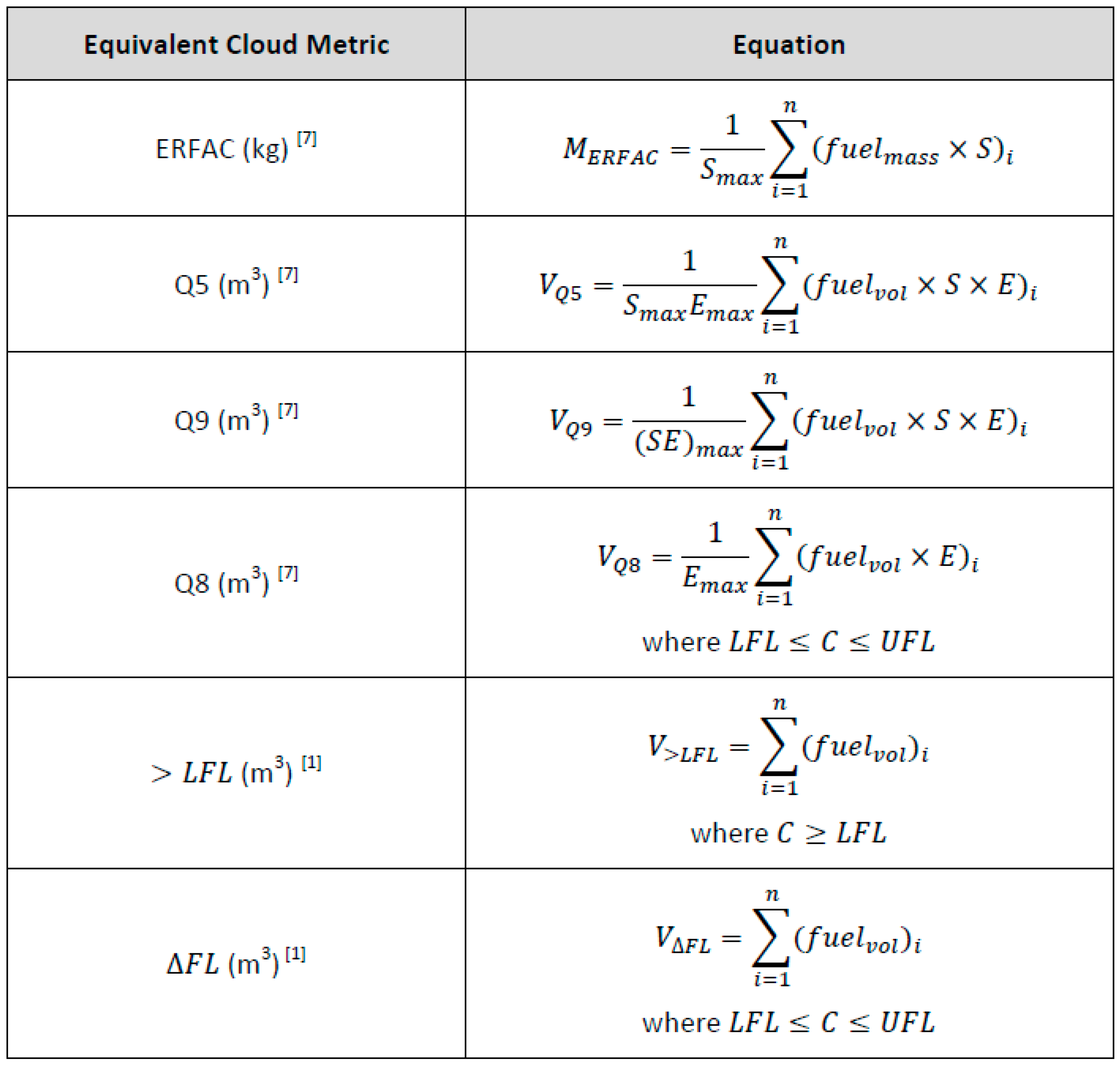
GexCon developed ESC models based on flame speed and expansion ratio; starting off with the simplest ERFAC, then Q5, Q8 and Q9 (see Figure 2), progressively increasing the effect of the gas concentration and expansion ratio in the model that defines ESC volumes. These names may appear esoteric; they are taken from variable names used in the Flacs engine. Flacs refers to the numerical explosion simulator. The whole modelling package including pre and post processors is called FLACS. The logic behind this is that it is known that the severity of a gas explosion depends on flame speed which varies with gas concentration.
There are simpler ESC models, such as “>LFL” (volume bounded by LFL) and “∆FL” (volume bounded by the upper flammability limit (UFL) and lower flammability limit (LFL)). They were used by BP following their analysis of large-scale experimental data. Definitions of these ESC models are given in Figure 2.
Presently, Q9 is used widely, other models (e.g., “∆FL”) have only a few users. While there are slightly more complicated methods for flammable volumes which can be transformed into ESC volumes (e.g., a workbook approach [14]), they are hardly used.
3. Underlying Assumption of ESC Methodology
There is an unstated assumption in the current use of ESC (i.e., dispersion-based ESC): that a real flammable gas cloud (with complex distribution of concentration and turbulence) is equivalent to a uniformly mixed stoichiometric flammable gas cloud in quiescent state (Figure 1). There is no theoretical basis or conceptual scientific deduction behind this assumption. Put simply, it is purely an assumption created for expediency (untested prior to the Phase 3B JIP [17]). In many engineering applications, this approach is acceptable when this is backed up by experimental data, leading to an empirical relationship that can then be applied more generally.
Hence, the evaluation of the ESC model performance against experimental data is important.
4. Case for Re-Assessment of Q9
Q9 is widely used, and a de facto standard method for CFD particularly FLACS [3,18]. There is a widely held view that Q9 is over-conservative; we frequently see this assertion in reports submitted to us for review. Part of this justification is that Q9 is recommended (i.e., in the FLACS user guide/manual), the other is the scientific basis of the model which includes some of the obvious physical processes involved. However, the evidence supporting this is not clear cut. There are two papers which give opposite conclusions: The Hansen paper published in 2013 [3] supports the current widely held view, while a paper by the authors published in 2008 [2] gives an opposite conclusion. It is interesting to note that the former paper [3] stated that Q9 is conservative upfront but did not provide evidence in the paper to support it.
Both papers derived their results using different methods; this makes direct comparison difficult. Ref. [2] presented only a comparison of overpressures between data and FLACS results based on Q9 cloud volumes derived from experimental gas concentration measurements. Results presented in [3] were based on simulation of non-homogeneous cloud formed from jet releases and did not involve Q9. The assessment of the performance of Q9 in the Hansen paper relied on a “good” correlation between overpressure data and Q9 volumes from concentration data. However, statistics of the correlation were not given. The Q9 simulations that were presented were not based on “realistic scenario” experiments. Thus, there is no direct comparison.
In addition, the results of the two papers were presented in different formats. While [2] presented them in MV (mean-variance) diagrams (described in more detail in Section 5.4) as recommended by the gas explosion model evaluation (MEGGE) project [19]. Hansen et al [3] presented results in the form of comparisons between observed and predicted pressure readings on selected tests. Therefore, it is difficult to compare the results of these two papers. This problem was highlighted by the UK Health and Safety Executive recently [15].
To avoid any confusion, it is necessary to carry out a comprehensive analysis. For consistency, we compared results from these two papers and additional analysis on MV diagrams. An MV diagram is a common format recognised in all model evaluation protocols [19,20,21] and that used in the BFTSS JIP Project model evaluation exercise [22].
5. Methodology
5.1. Dataset from Phase 3B
A major part of the Phase 3B of the Blast and Fire for Topside Structure joint industry (BFTSS) project (henceforth referred to as Phase 3B) was a large-scale experiment designed to study realistic scenarios involving the release of high-pressure natural gas into a large-scale model of an offshore production module [17]. Phase 3B provided realistic release scenario data for the development and evaluation of gas explosion models. Both papers ([2,3]) used this dataset.
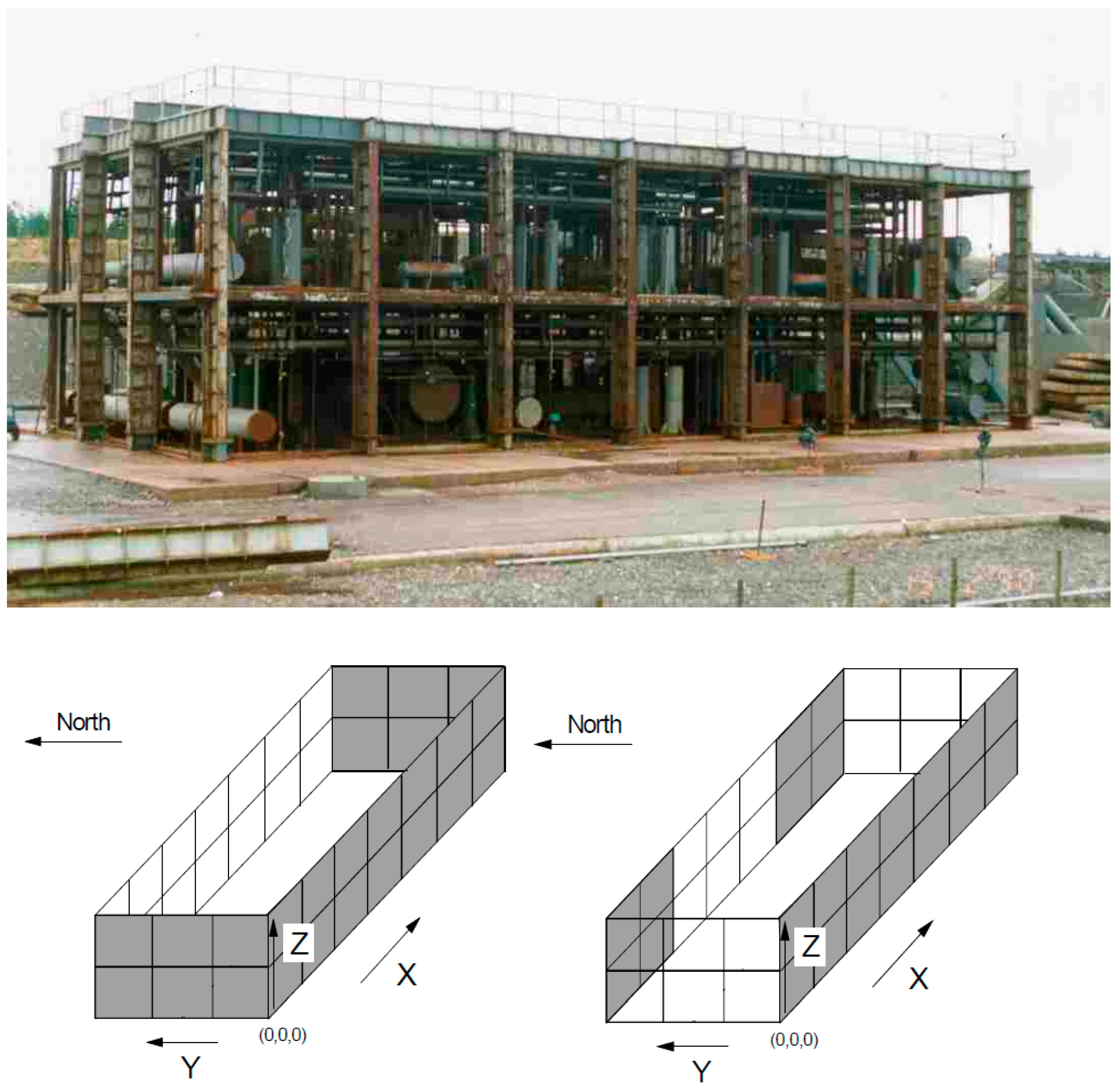
The whole Phase 3B project consisted of laboratory, medium and large-scale tests. Only the large-scale experimental dataset is used in this paper. Figure 3 shows the experimental test rig which measured about 28 m long, 12 m wide and 8 m high. It was a simplified full-scale model of a compression module on a platform operating in the North Sea at the time. Natural gas was released within the module. The release rate was held constant within each test until gas concentrations and their distribution inside the module reached a steady state prior to ignition. Release rates varied between 2.1 kg s−1 and 11.7 kg s−1 in the Phase 3B programme. Release directions were in line with one of the three orthogonal coordinate axes of the test rig. In total, twenty tests were carried out. Gas concentrations were measured at 50 locations prior to ignition and overpressure at 25 locations distributed inside the module. Earlier phases of the BFTSS JIPs are not relevant for this paper. The earlier phases provided an interim engineering guidance note [23] and data from experimental programmes addressing theoretical worst-case and specific worst-case scenarios (for model evaluation), and mitigation options [12,19].
5.2. Previous Work on Flammable Volumes
Just before the Phase 3B JIP, the Dispersion JIP [24] studied the dispersion of releases of pressurised natural gas in the same large-scale module as Phase 3B. ESC models of “>LFL” and ∆FL were evaluated and compared with predictions from FLUENT [25] (and FLACS [26]. These papers showed that both FLUENT and FLACS were able to estimate “>LFL” and ∆FL with little bias. Q9 was not part of the evaluation.
The results of Hansen et al., 2013 indicated that FLACS also could predict Q9 with little bias.
5.3. Versions of FLACS Used
The underlying physics of the explosion code, Flacs, has changed little during the period since the completion of the Phase 3B JIP. FLACS has undergone many development iterations. Significant effort has gone into making the code easier to use, numerically more stable and faster to execute.
Three different sets of results on Q9 had been published in 2001, 2008 and 2013 using FLACS version current at the time. Further data were generated for this paper using the latest version of FLACS.
We compared gas explosion results on selected project work in BP using the current version FLACS 10.6 with FLACS 8.1 which is close to FLACS 99 r2 when GexCon first carried out a comparison of FLACS with Phase 3B data [17].
A point to point comparison gave differences of less than 5% between the “old” and the current version of FLACS. On average, the current version gave slightly lower prediction at pressure above 2 bar and slightly higher below it. These differences are insignificant for our purpose here.
5.4. Format of Comparison—The MV Diagram
The results are presented in MV diagrams in this paper. The MV diagram shows two quantities: geometric mean (MG) and geometric variance (VG). Their definitions are given in [2] and summarised here:
where:
MG = exp (<ln( P/O)>)
VG = exp (<(ln(P/O))2>)
- P = predicted overpressure
- O = observed or measured overpressure
- <X> denotes expectation value of X
The position on an MV diagram shows the overall performance of mathematical models (in this case ESCs) based on results of comparing large number of simulation—experiment pairs.
An MV diagram gives two important measures: bias and variance. Bias shows whether a model systematically under or over predicts experimental results overall; however, bias does not tell you how likely the results are to over or underpredict data in any one simulation situation; variance provides an indication of this.
Variance shows the range of scatter about the mean. A model with a large bias may appear to be a poor tool; however, a correction factor could be applied in practice if the variance is small. A model which has a large variance is unreliable irrespective of bias; results are difficult to interpret, and no simple correction factors can be applied.
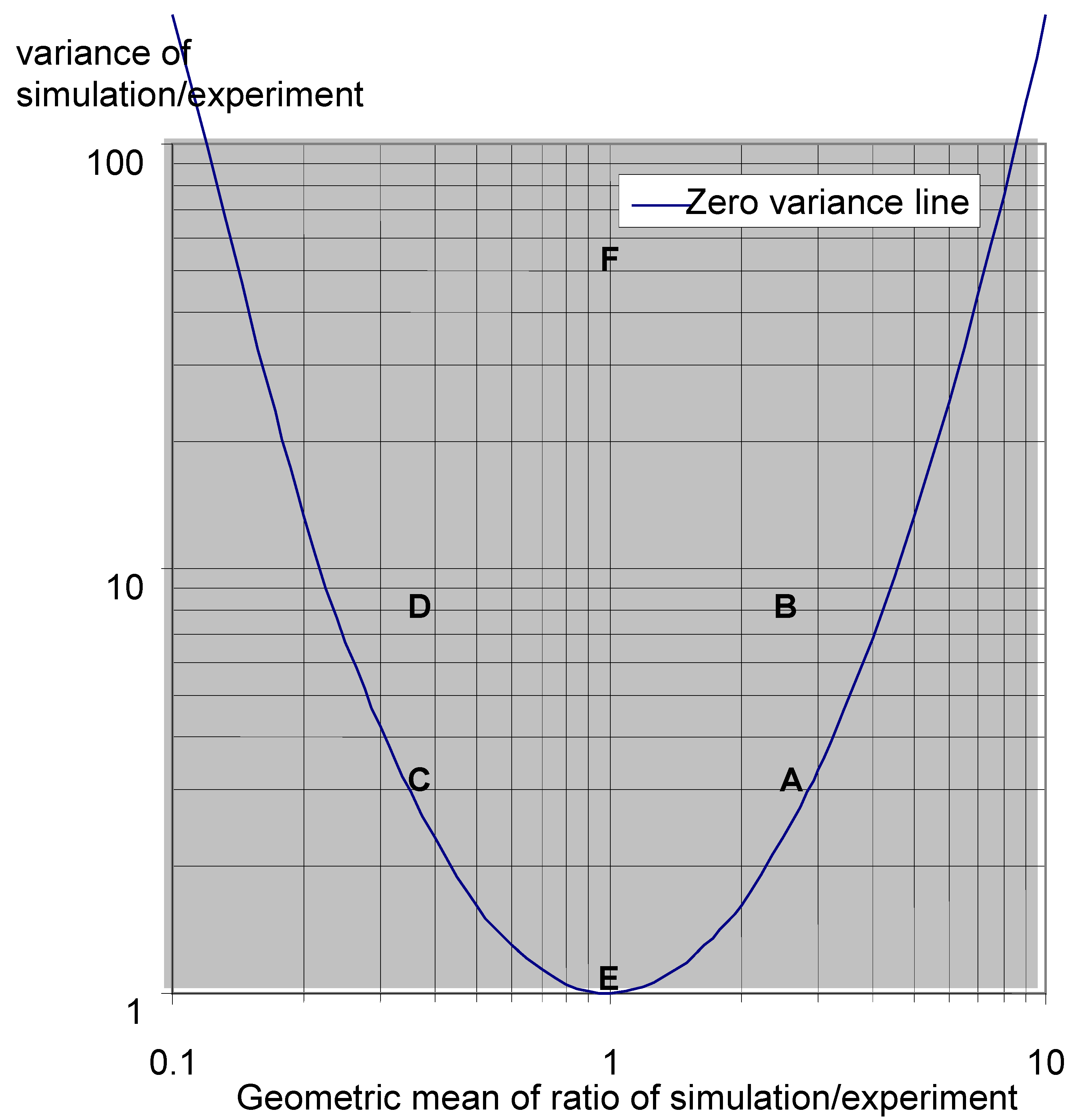
An ideal model will be neutrally biased (with a geometric mean MG of one) and a variance (geometric variance VG) of one on the MV diagram. This corresponds to a situation where a model accurately predicts experimental outcome/data with no error every time. Position E shows the position of such a perfect model on the MV diagram (see Figure 4).
Continuing with Figure 4, position C shows the relative position of a model with bias MG much less than 1 but with a small variance VG, indicating the model is underpredicting data systematically and consistently. Position F is for one with MG close to 1 showing that there is no systematic bias, but it has a large VG. This means that the model in position F produces unreliable results which can wildly under- or over-predict.
There are many reasons MV diagrams are preferred in model evaluation protocols. They are described in detail in [27]. Here are a couple of key considerations:
- (a)
- Scale
As the range of experimental data spans more than three order of magnitudes (from millibars to tens of bars), predicted-over-observed graphs tend to have data points bunching together into groups. The alternative of using log plots compresses deviations making agreement better than superficial appearance suggests.
- (b)
- Ease of comparison of the two key characteristics of model predictions
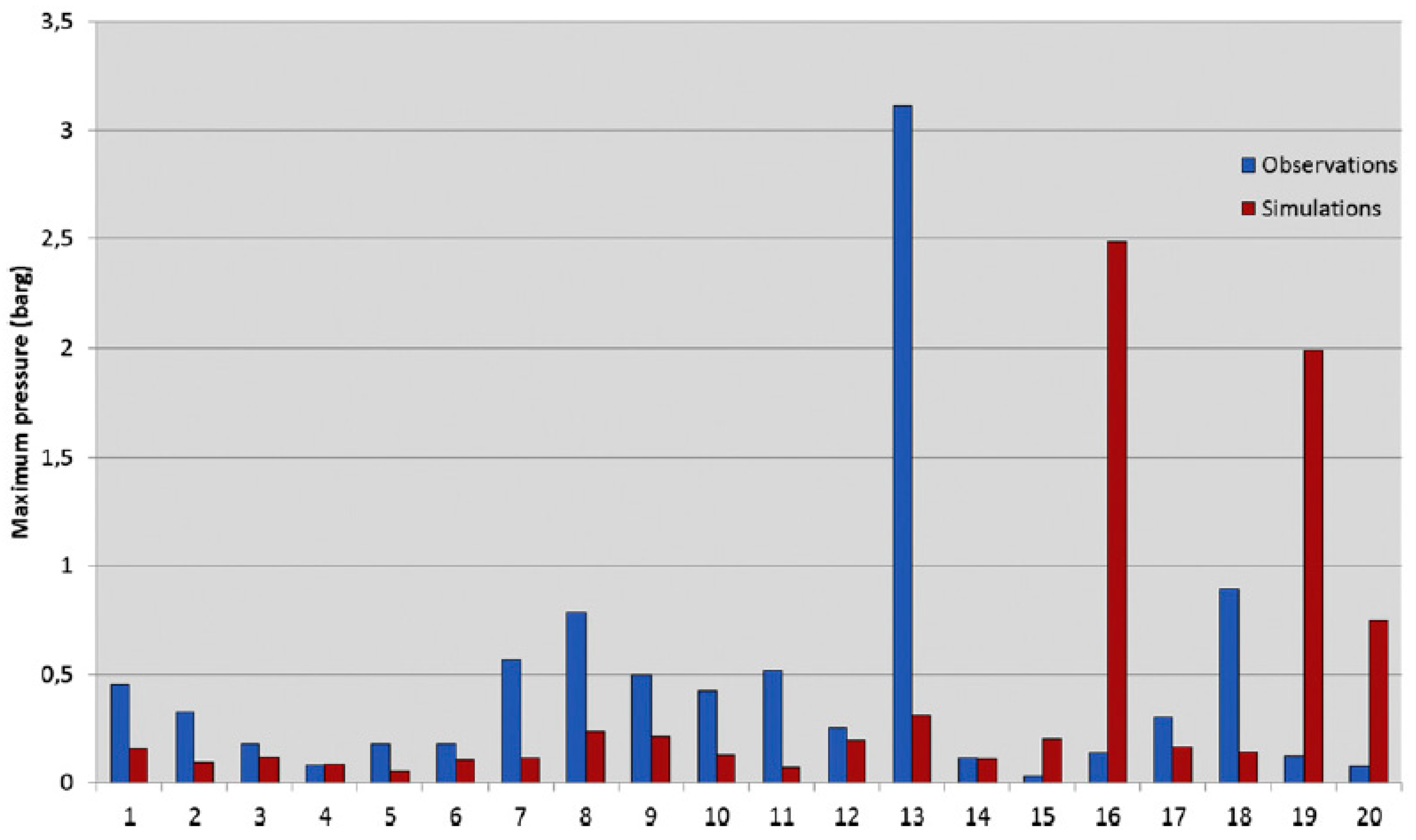
There are many statistical methods for comparing predicted and observed results, such as quantile–quantile plots, residual values, scatter diagrams, bar charts, etc. While they are useful in detailed examination of model behaviour/characteristics, they contain too much information. Figure 5 is an example which shows model comparison results between predicted and observed. It is difficult to pick up visually relative biases and variances from it.
6. Results and Evaluation
6.1. Estimation of Overpressures by Direct FLACS Dispersion-Explosion Simulations
One method of calculating explosion overpressure in a realistic scenario is to use the results directly from a dispersion calculation, without involving any ESC model.
A large part of the results presented by [3] was based on this methodology. This involves calculating the evolution of a flammable gas cloud from a known release source (with known orifice diameter and release rates) and release conditions. An electric spark ignites the cloud once it has reached a steady state. This methodology does not require the use of Q9 or any ESC models. There are two sources of data: (a) Figure 5 (top), and (b) the Phase 3B report [16].
A summary of the results is given in Table 1.
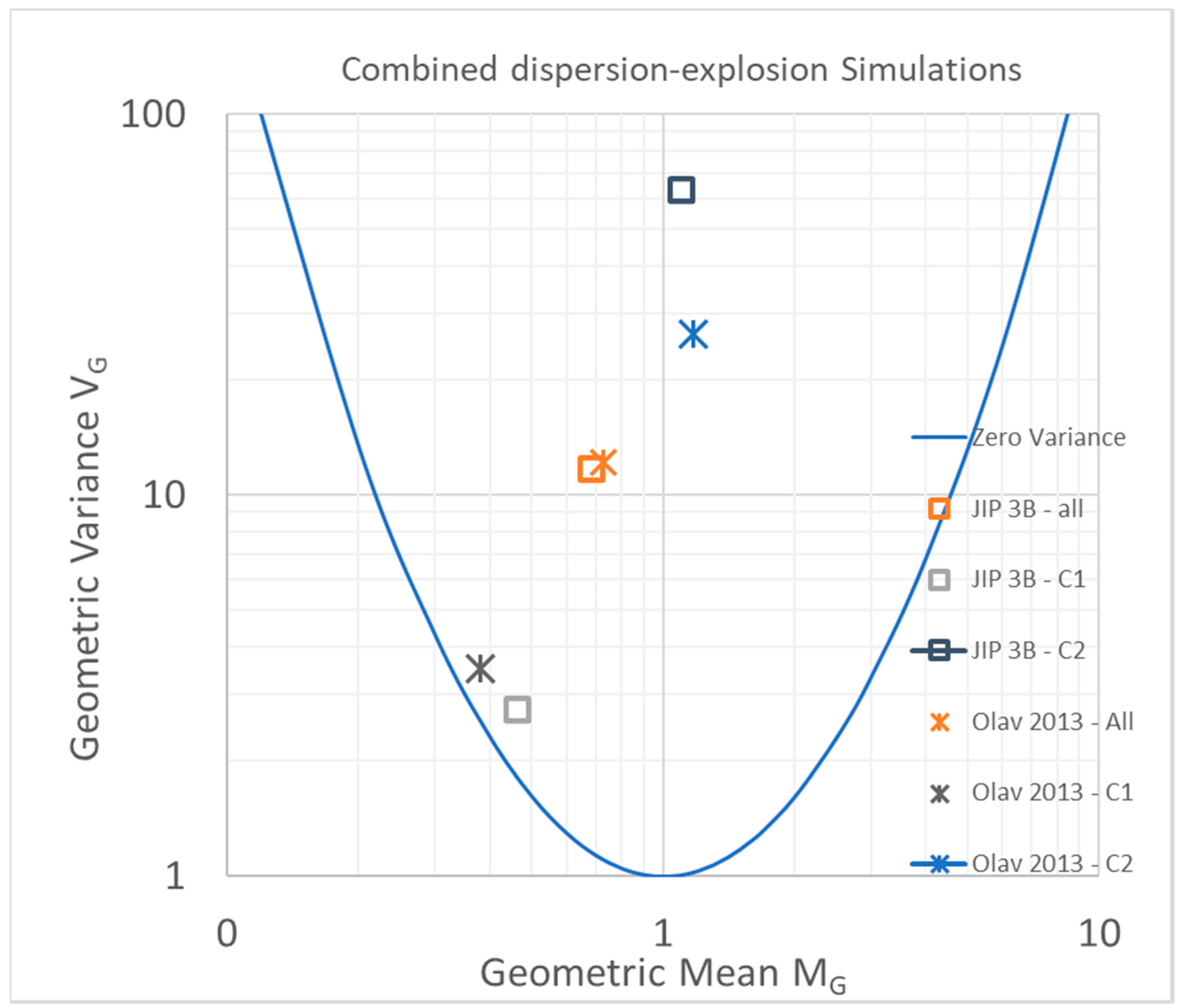
The Hansen 2013 [3] result gives an overall geometric mean (MG) of 0.73 and a geometric variance (VG) of 12. Though the underprediction is modest, the variance is large. Dividing the dataset into the two layout configurations C1 and C2 in the large-scale tests (see Figure 3), the corresponding MG and VG values for C1 are 0.38 and 3.5 and for C2 are 1.2 and 27. The underprediction is more severe for C1 than that for the complete dataset and with a reduced variance. However, the results for the C2 layout gave overpredictions instead with a much-increased VG. These results indicate considerable dependency on the layout of solid wall boundaries.
The results from the two studies spanning a decade are consistent with each other in that C1 was consistently underpredicted with a variance in the mid to low single digits, and C2 was consistently overpredicted and with a very large variance.
An MV diagram showing a summary of these results is given in Figure 6.
Effect of Control Volume Sizes—Grid Dependency for Dispersion-Explosion Linked Simulations
The effect of grid sizes on the simulation results is significant. Data issued by GexCon as part of the Phase3b JIP showed results for three grid sizes: 0.5 m, 1 m and 1.33 m; these are grid sizes outside the grid refinement zone. The refinement zone is the region immediately around the gas jet in order to obtain more accurate estimation of jet behavior through resolving flow details better. This zone contains a range of grid sizes smaller than those outside this region. A summary of the results is given in Table 2.
The results show significant dependency on grid sizes, see Figure 7. As grid size increases, the bias worsens; MG values move from 0.68 to 0.54 to 0.3 for grid sizes of 0.5 m, 1 m and 1.33 m, respectively. Variance also increases with grid sizes indicating that the model results become increasingly unreliable. The two subsets of data for the C1 and C2 layouts show similar trend with higher values of variance.
The results shown in Table 1 indicated that the results of Hansen 2013 were mostly likely based on grids of order 0.5 m.
6.2. The ESC Model—Q9
The methodology in explosion hazard assessment using the Q9 model involves two steps: (a) calculating a flammable volume and (b) locating the Q9 gas cloud in various locations for the purpose of determining maximum overpressures.
6.2.1. Cloud Volumes Derived from Experimental Data
Results are summarised in Table 3 which gives the maximum calculated overpressure of any of the sensor locations against maximum measured overpressures of any sensors. This was for Q9 volumes derived from experimental gas concentration measurements.
Table 3 also contains additional results on averaged overpressures. They give the averaged values of all maximum pressures of all sensors compared with the average of maximum pressures calculated at all sensor locations within the module. Generally averaged values have marginally smaller MG and smaller variance; this is as expected.
As stated in the Tam 2008 paper, the results showed that when all the data are considered, the Q9 model is neutrally biased. This is reflected in the results in Table 3.
6.2.2. Cloud Volumes Derived from FLACS Dispersion Simulations
This reflects how ESC is used in ERA in practice. Q9 volumes are calculated by FLACS which sums up Q9 volume contributions from every grid cell within pre-defined boundaries of the area of interest (e.g., a compression module on a platform).
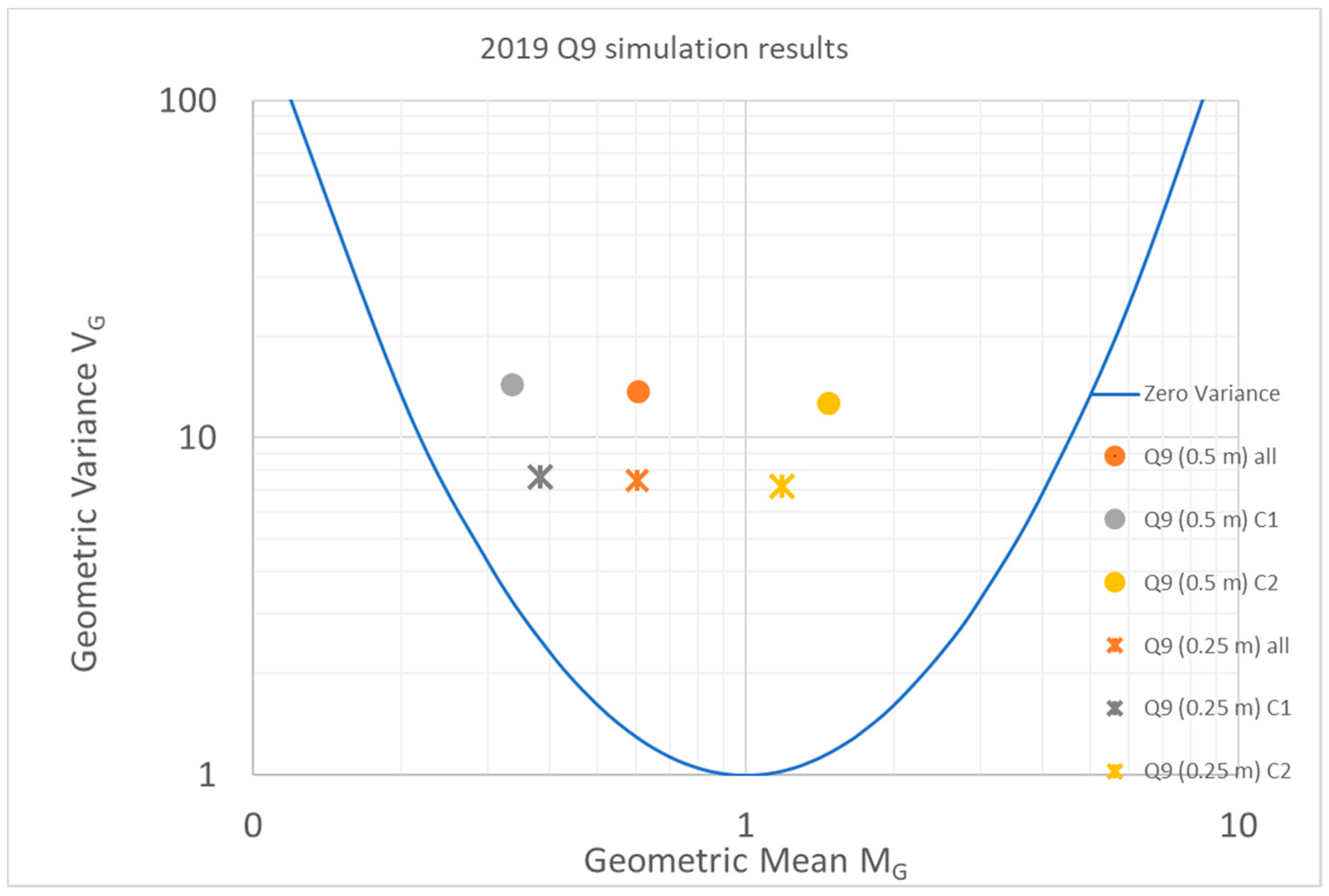
This work was carried out in 2019. As previous work indicated sensitivities to grid sizes, we decided to calculate overpressures using two grid sizes: 0.5 m and 0.25 m. It would have been necessary to apply more than these two grid sizes in practice during an ERA due to the range of ESC volumes being considered. A summary of the results is given in Table 4.
The trend of results of “All”, “C1” and “C2” are consistent in all the results above, in that “C1 only” results are underpredicted and “C2 only” results are overpredicted. Over the entire dataset, the Q9 model led to underprediction. Specifically, on this set of results, it can be seen that the smaller grid size of 0.25 m gave better quality results: the range of bias is reduced, and the magnitude of variance is nearly halved.
Figure 9 summarises the results.
6.3. Sensitivity to Cloud Locations
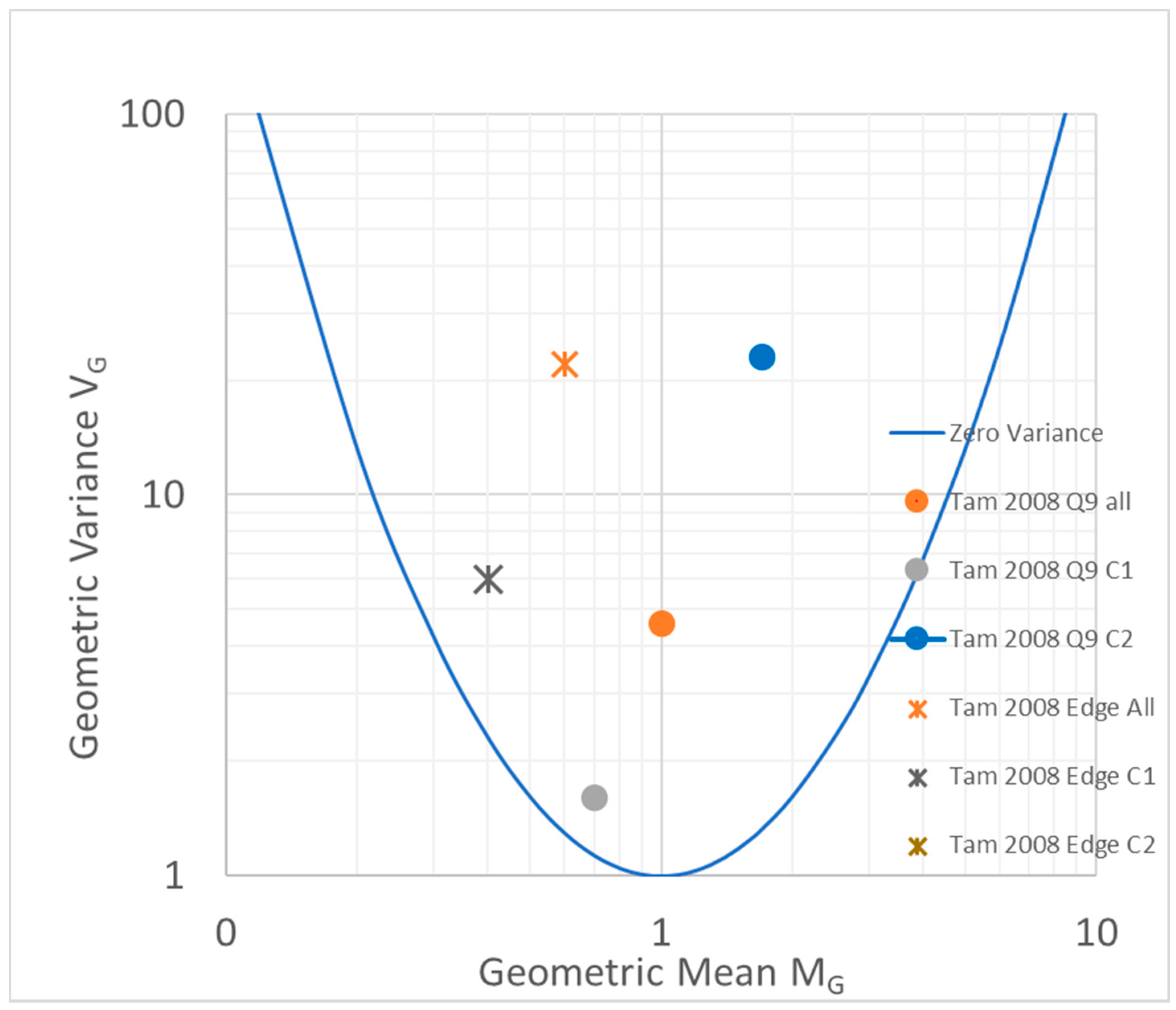
Predicted overpressures are sensitive to where the Q9 cloud is placed. This was discussed in [2] in which authors compared calculated overpressures of ESCs placed at the centre of the test module with those located at the edge. The average ratio was found to be about three.
The sensitivity to location is shown by the associated variance VG which has a higher value than those sited in locations for highest overpressures (see Figure 8).
Results indicates that this sensitivity tends to be higher for the ESC model that produces smaller cloud volumes than those which produce larger volumes. For example, the ESC model, “>FL” or ∆FL, produces larger cloud volumes than those from the Q9 model; they show less sensitivity [2].
7. Discussions
7.1. Consistency of Results
All the results calculated over the last two decades using various methods of deriving Q9 volumes have the same behaviour: Q9 underpredicts in all of them when the whole Phase 3B dataset is used, and the trend in predictions for the two layout configurations is consistent.
7.2. Sensitivity of FLACS to Boundary Properties
While this is not the main objective of this paper, the Q9 results show that there is a strong sensitivity to layout of boundary walls. In the two configurations in Phase 3B, the C1 configuration (see Figure 3) is close to a “tunnel” type layout with two parallel walls and the prevailing wind direction being along the length of the module, while the wall arrangement in C2 is a U shape with the open U on the long side. Wind direction was always along the length of the experimental module. In the C1 layout, wind flowed through the two open ends of module (Figure 3 bottom right). In the C2 layout, wind blew across the open side (Figure 3 bottom left). The results strongly suggest that as the wall arrangement deviates from a tunnel arrangement, the Q9 model becomes more unreliable as shown by the large value of variance VG.
7.3. Reliability of Direct Dispersion–Explosion Simulations
This method suffers from excessive variance, and sensitivities to grid sizes and wall layout.
Like all CFD codes, FLACS is susceptible to grid size sensitivity. GexCon has made significant effort to limit its effect, e.g., there is a firm guidance on grid sizes for explosion simulations. However, the guidance for direct dispersion–explosion simulations does not exist. As results here show, this direct dispersion–explosion methodology performs poorly and is prone to grid sensitivities. As it is, there is no justification of using this method: it is less accurate and more costly.
Further validation and guidance are clearly needed.
7.4. Q9 Is Not Conservative
Hansen et al [3] asserted repeatedly that the Q9 model is conservative and that all other methods are excessively conservative. They imply that Q9 is conservative through an indirect comparison with data. However, their own conclusion did not support their own assertion: “Pressures achieved when exploding quiescent Q9 based ideal clouds correlate quite well to experimental pressures from ignited jets, but for some test scenarios higher pressures are seen than obtained with the quiescent ideal clouds”. At best, Their own conclusion indicates that the Q9 model is neutrally biased.
Results of this paper and [2] do not support the “over conservative” assertion.
7.5. Complexity and Accuracy
We found that many of these assertions on “conservatism” are based on theoretical argument, sensitivity calculations or “experience”. The misconception is that a method or a mathematical model containing some physics must be more accurate and better than methods containing less. The devil is in the physics that are missing. Complexity should not be confused with accuracy. This was discussed in [2].
7.6. Key Learning
7.6.1. Recommended Usage of Q9 Is Inadequate
Hansen et al.’s recommendation is that only the calculated maximum overpressure values (over the entire volume of interest and across all ESC locations) are used for probabilistic assessment for each release scenario (e.g., producing exceedance curve): this approach would be conservative. It could be. Only if Q9 is unbiased.
However, results show that the Q9 model systematically underpredicts, hence the assertion of conservatism does not hold. Secondly, this recommendation is not universally applied in practice in ERAs. We will discuss the effect of conservatism or lack of it next.
7.6.2. Applications of ESC in Probabilistic Explosion Analysis to Exceedance Curve
It is common to use a risk-based approach to define explosion loads for structural design. The design accidental load (DAL) is an example of this. DAL is widely used, and its value is derived from an exceedance curve. DAL is defined as the explosion load on a structural element for a specific cumulative risk frequency which can be obtained from an exceedance curve. This is based on the limit state approach in the design of structures against gas explosions [28,29]. This approach was based on an established methodology on design against extreme environmental loads such as earthquakes and ocean waves. This is now encapsulated in the Fire and Explosion Guidance [18]. It recommends that design loads correspond to two limit states, strength level blast (SLB) for frequent, and ductility level blast (DLB) for rare events, respectively: the former ensures integrity which minimises structural and equipment damage that could lead to prolonged operation disruption, the latter for protection of people through avoidance of progressive structural collapse. This guidance is consistent with that in NORSOK Z-013 and ISO 19901-3. The threshold of cumulative frequency for DLB varies. The guidance defined a minimum of 10−4/yr, and some companies chooses the other lower bound, e.g., 10−5/yr in order to keep total risks from both fire and explosion to below 10−4/yr.
The effect of systematic biases of an ESC model can be significant. For example, the DAL derived from exceedance curves or explosion risk analysis could be underestimated if the ESC is systematically underpredicting.
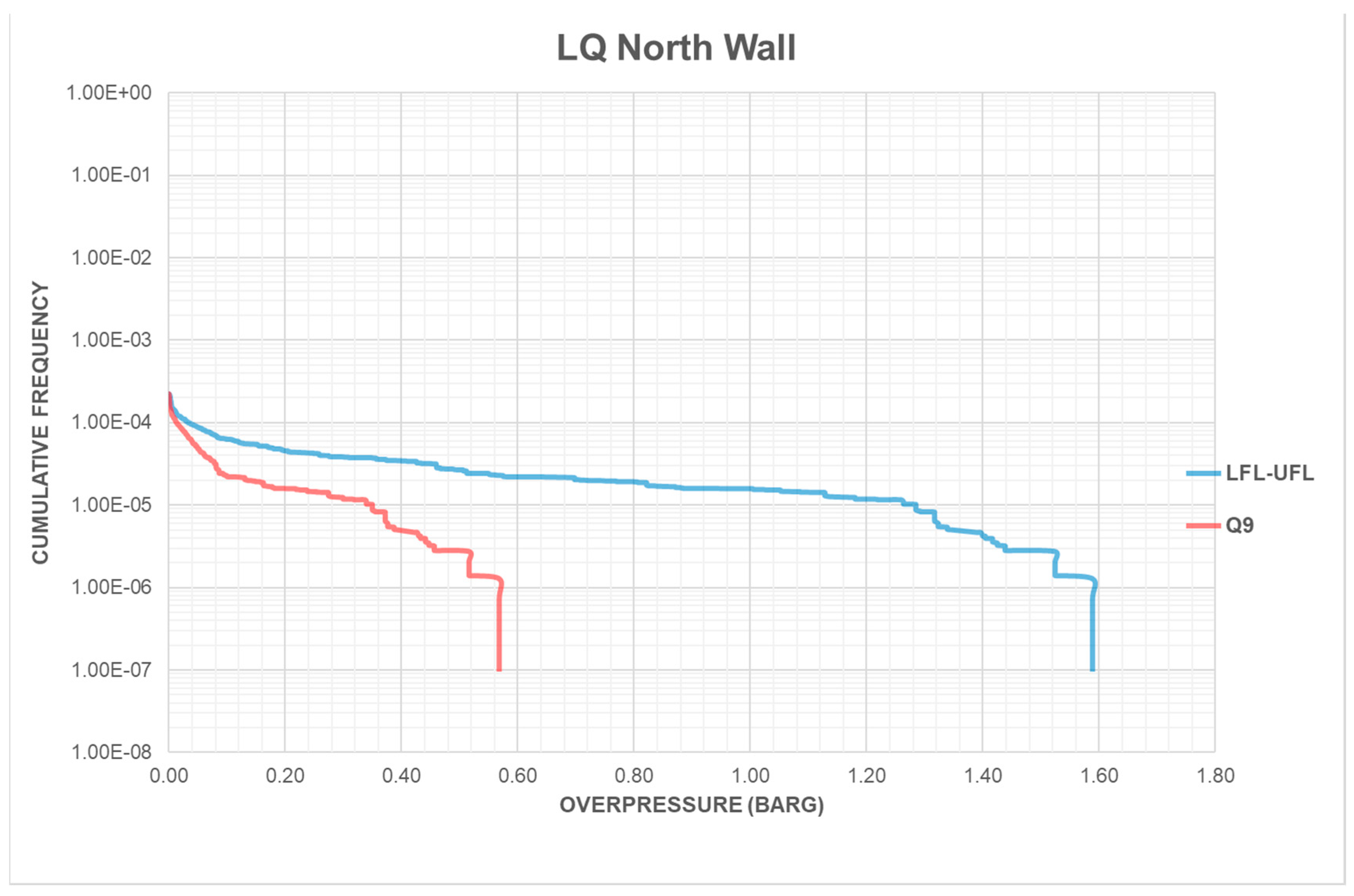
This can be illustrated by comparing exceedance curves derived from two ESC models. This example is taken from a study that we undertook on an existing facility. We calculated the DAL values for a structural wall using the two ESC models, ∆FL and Q9. Figure 10 shows the two exceedance curves derived from them for a wall on the living quarter. It can be seen that there are significant differences between them. The key points illustrated in the figure are:
- (i)
- The DAL derived from the Q9 model is more than three times smaller than that from the ∆FL model, e.g., 0.4 bar and 1.3 bar, respectively at a cumulative frequency of 10−5/yr. The magnitude of DAL varies according to the level of exceedance set. At 10−4/yr. The magnitude of overpressure is much lower, though the ratio remains similar.
- (ii)
- The maximum overpressure calculated also varies about three-fold: 1.6 bar compared with 0.6 bar for the ∆FL and Q9 models, respectively. This higher maximum overpressure is probably not used for structural design of the blast wall in a risk-based approach. However, there are impacts on hazard management, e.g., on (a) emergency planning and management and (b) siting and layout particularly for onshore facilities at an early stage of design, e.g., the concept selection stage.
The results presented serve to highlight the choice of an ESC model can have a significant impact on design and risk management. An ESC model that systematically underpredicts will also underpredict DAL.
This could lead to inadequate design of blast walls and other critical structures.
7.6.3. Recognised Evaluation and Presentation Format
When presenting results, a recognised and common format should be used. Over-complex figures with lots of data points are confusing, not to mention there are many data points which overlap, and true results are obscured.
7.6.4. An Explosion Risk Assessment in Practice
The current guidance for explosion modelling in FLACS requires that there be a minimum number of control volumes across the minimum dimension of an ESC. As some of the Q9 volume can be small, two issues arise:
- (a)
- Adherence to guidance: this would require carrying out simulations using different grid sizes depending on results of dispersion calculations. As a typical ERA involves large numbers (of order a 1000) of simulations, there is a temptation to bypass or approximate this step given time and cost pressure.
- (b)
- The effect of mixing or using different grid sizes is difficult to quantify—as can be seen above, FLACS is grid sensitive. The net effect of mixing results obtained using various grid sizes has not yet been quantified.
7.6.5. Quality Control Issues
Best and common practice implementation across the consultant industry is an issue. Our experience from reviewing reports from a range of consultants is that rigorous quality assurance by company or independent experts is necessary as ERA processes and procedures involved in the application of the Q9 model vary and the impact of this difference is not obvious and usually not stated. This issue is not new [30]. A recent JIP proposal by the UK Health and Safety Laboratory goes some way to address it [15].
7.7. More Recent Data on Hydrogen
The Q9 and other ESC models described here were developed for hydrocarbons. The burgeoning of hydrogen economies would demand similar assessments as those for the hydrocarbon economy. Application of any ESC model for hydrogen should be verified by data from full scale hydrogen experiments.
Data from Phase 3B are not appropriate.
Current “validation” results based on hydrocarbon cannot be carried forward to applications to hydrogen. Appropriate hydrogen data should be used to calibrate ESC models. We understand that there are recent and ongoing research programmes which provide near full scale data for specific applications (e.g., on hydrogen filling stations, [31,32]).
7.8. Application of Q9 in Reality
The comparison so far is based on maximum values among all sensors in the experiment with maximum calculated values selected from those sensor locations, i.e., the maximum of all sensors against the maximum of all monitoring points. A monitoring point is a location in the calculation domain where values of fluid properties are extracted or “monitored”. In this case, the monitoring point locations duplicate those in the experiment. The recommendation of the use of the Q9 model is aligned with the validation methodology. That is, only the maximum calculated values from all possible locations of Q9 clouds are used.
This is akin to using CFD models as though they are simple empirical or phenomenological box models which are much simpler and cheaper to run.
The issue is a philosophical one. What is the point of using a complex and expensive code when you cannot use all the other results generated? The temptation to utilise volumes of detailed calculation results is overwhelming, particularly for the uninitiated. Unsurprisingly, more and more complicated analyses are developed, utilising the vast amount of calculated values for other parameters. We will explore some of these analyses later.
7.9. Expectation and Reality—Application Outstripping Capability
Expectation of the capability of commercial explosion codes like FLACS is high. There is a danger that expectation outstrips the capability that can be realistically delivered. We will explore some examples with the application of the Q9 model.
In common with other CFD codes, FLACS produces many details, showing distribution of pressure in space and in time as well as other useful parameters such as velocity, drag forces, etc. The availability of this information often leads to changes in assessment methodologies impacting on design. While published validations have been on global values (e.g., maximum (or mean) among measurements) of a limited set of model outputs, there is no published systematic validation exercise on their spatial and temporal distribution that we are aware of.
Our observation is this. The mere fact that output of these other model parameters is available will lead to their use in practice. When one aspect of the code is deemed to be validated, it is then assumed that the whole code is validated covering other aspects beyond the limited validation exercise.
Here, are two examples to illustrate the point.
7.9.1. Refinement of Transient Nature of Releasees
As large releases tend to be short-lived due to finite inventories, releases from large leaks tend to reduce with time, e.g., as a blow down system is activated or inventory depleted. There is an increasing use of the time-varying characteristics of the transient nature of hydrocarbon releases to define a more “accurate” risk value. This is done by integrating instantaneous risk values over the period of hydrocarbon release. The incorporation of the transient effect usually results in lower risk figures than steady release over the release period.
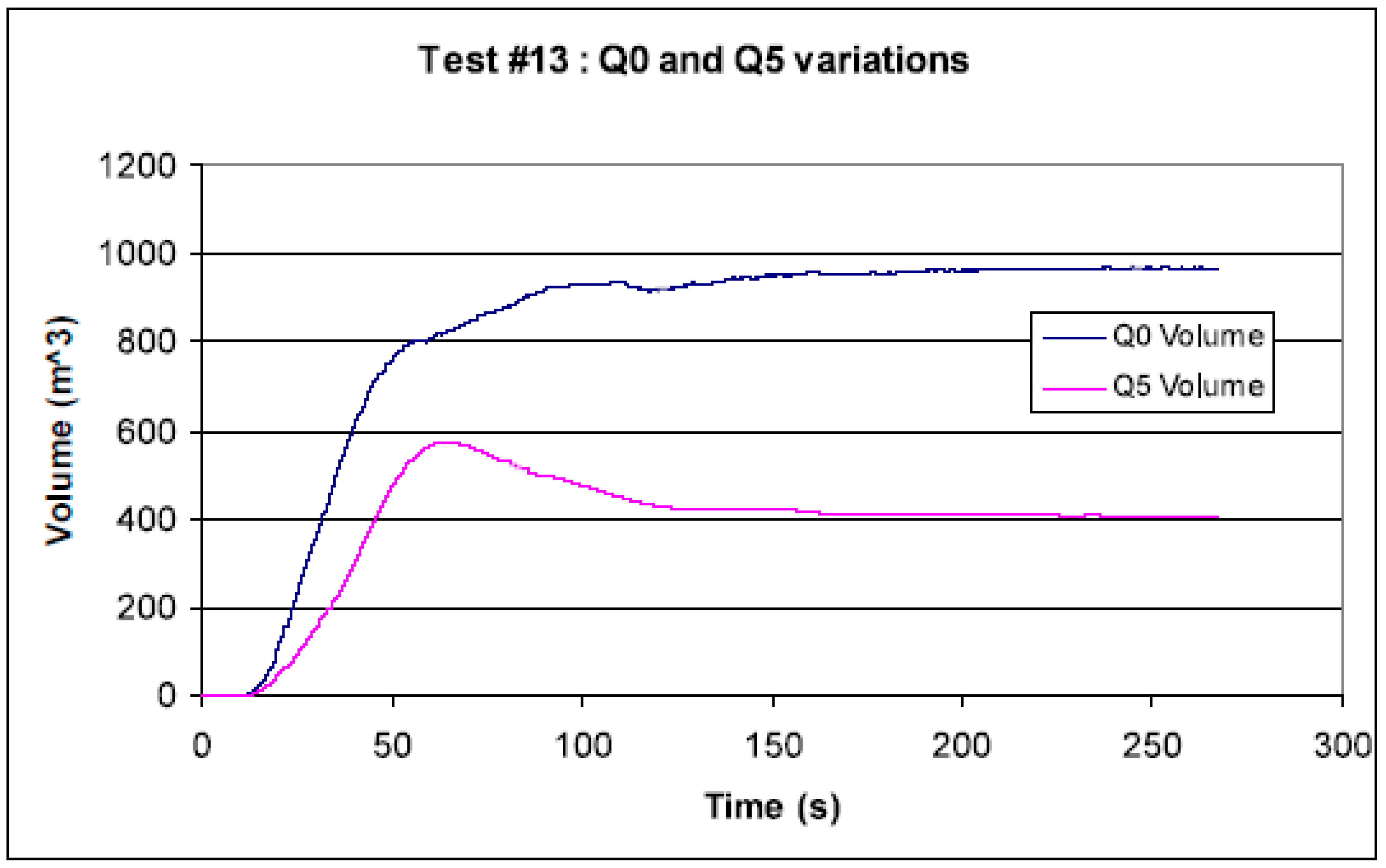
The integrated risk values are sensitive to the choice of ESC model. Q9 cloud volume–time history has a common characteristic in that with an initial peak the cloud volume decays more or less monotonically with time (see Figure 11). Other ESC models may not share this. This is illustrated by comparing ESC volumes from two models: Q5 (Q9 and Q5 are very similar in definition (see Figure 2) and Q0 from the FLACS simulation of Test 13 in Phase 3B [17], see Figure 12.
The evolution of these two ESC volumes with time is very different. In this example, the Q9 model would predict an integrated risk of more than half that derived from Q0 assuming uniform ignition probability with time.
We highlighted this aspect here because the maximum volume and subsequent evolution of flammable volume depend on the choice of the ESC model. There has not been a study on the validity of any ESC model for this application.
7.9.2. Advanced CFD/FE Analysis
There is an increasing trend to make use of detailed output from FLACS to “optimise” structural design. The spatial and temporal distribution of pressure results are extracted, and this is applied as direct input to a finite element structural response code so that the temporal and spatial characteristics of the load are accounted for in the structural response.
If there is validation of model predictions on spatial distribution with time and the performance is good, the adoption of this approach would have been compelling. However, this validation has not been carried out. There were some limited study for theoretical worst-case scenarios on coupled loading–response analysis [11,33].
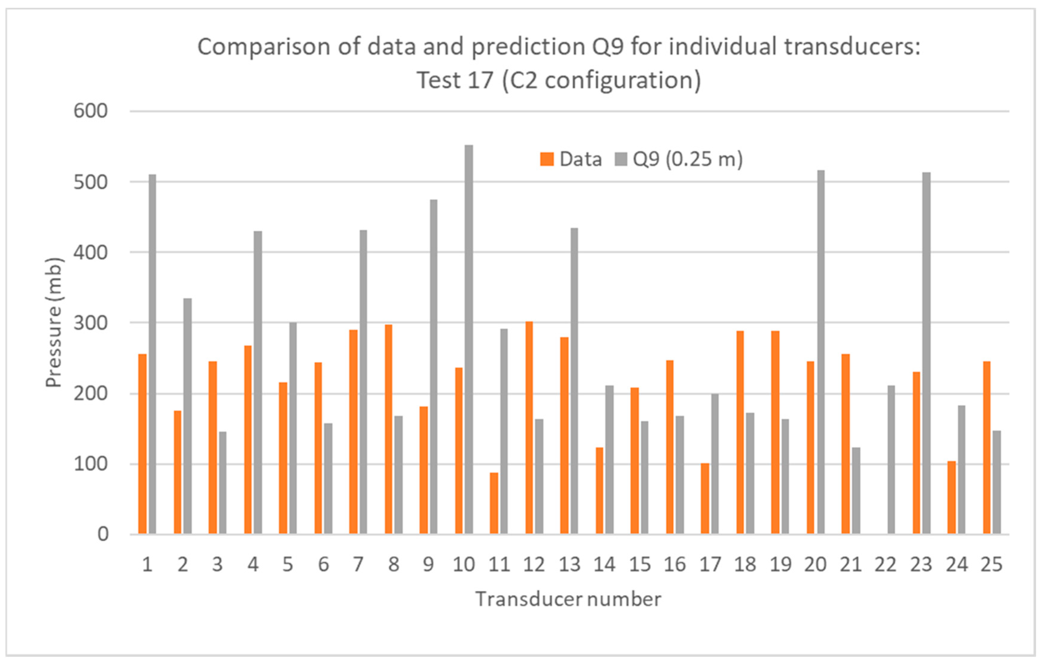
Our analysis shows that there is a large variance (VG) associated with model predictions, as shown above in Section 6.1. Figure 13 is a comparison of predicted and observed maximum overpressure at all sensor locations for Test 17. We chose this test because the Q9 model gives the best match between data and simulation results. The figure shows that there is a large variation between predicted and observed maximum overpressures at each of these sensor locations.
Our results here show that the variance of predictions against measurements for individual points is much higher than those of global maximum against global maximum or global average against global average results. It is possible that these variances when combined (with uncertainties associated with structural response analysis) all cancel out to provide an accurate or acceptable description of response. This has yet to be demonstrated.
We contend that the approach of mapping spatial and time distribution results onto structural FE code is susceptible to unquantifiable error. We suggest that development work and guidance on this application are needed.
8. Conclusions
A comprehensive review was carried out on previous work (from 2001) on comparison between data from the large-scale realistic release JIP (Phase 3B) and simulation results of FLACS using the Q9 model.
The Q9 model in FLACS significantly underpredicts the Phase 3B dataset. The value of the geometric mean (MG) is 0.6 for maximum overpressures. This has the effect of underestimating design accidental load, leading to inadequate design or underestimation of explosion risks.
Results also show that there is a large systematic difference in the Q9 model performance for the two wall layouts in Phase 3B—underprediction and smaller variance in the tunnel geometry compared with overprediction and higher variance in the U shape geometry.
9. Observations
- There is an assumption that the Q9 model is more accurate because it contains more physics than one containing less. This is not true. The devil is in the missing physics. The true arbiter is validation with full scale data.
- Recognition is lacking in the industry of the limitation of the code, and the lack of appropriate data and validation. As a result, ever more complex analyses are being carried out where there is no validation or detailed scientific evaluation to support them (e.g., time varying risk calculation, time and spatially coupled-load–response analysis on structures, etc.).
- Recognised model evaluation protocols should be used in all publications on model validation or model evaluation. This provides clarity and avoid confusion.
- The hydrogen economy is fast developing. The application of the Q9 model to hydrogen requires a separate evaluation/validation exercise based on hydrogen data derived from experiments at appropriate scale.
10. Recommendations
This study highlighted five main areas where further work is recommended:
- (a)
- Develop an appropriate ESC model through vigorous scientific methods and validated by appropriate scale data.
- (b)
- Q9 should be used with caution; a full account of systematic underprediction and large variance should be made.
- (c)
- Generate appropriate large-scale data with a wider range of conditions than those of Phase 3B, e.g., involving a range of geometries and boundary wall arrangements, and non-steady scenarios, such as simulation of blow downs and delayed ignition. The industry should form a JIP to address this.
- (d)
- The issue of variability due to users in the execution of ERA, particularly involving the Q9 model should be addressed. A JIP that goes someway to address this issue was suggested by the Health and Safety Laboratory on a joint ERA inter-comparison exercise involving key consultants [15].
- (e)
- The validity and applicability of coupled explosion loading/structural response analysis should be clarified. This could involve a guidance to define correct application, evaluation against data to establish confidence limits, etc.
Author Contributions
Conceptualization, V.H.Y.T.; methodology, F.T., V.H.Y.T. and C.S.; formal analysis, F.T., C.S.; investigation, F.T., V.H.Y.T., C.S.; resources, C.S., F.T.; data curation, F.T.; writing—original draft preparation, V.H.Y.T.; writing—review and editing, F.T., C.S.; visualization, F.T., C.S.; supervision, V.H.Y.T.; project administration, V.H.Y.T. All authors have read and agreed to the published version of the manuscript.
Funding
This research received no external funding.
Institutional Review Board Statement
Not applicable.
Informed Consent Statement
Not applicable.
Data Availability Statement
Not applicable.
Conflicts of Interest
The authors declare no conflict of interest.
Abbreviations
| ∆FL | Concentration between upper and lower flammability limits. |
| > LFL | Concentration above the lower flammability limit. |
| MG | Geometric mean. |
| VG | Geometric variance. |
| BFTSS | Blast and Fire for Topside Structure joint industry—the name of a series of JIPs spanning over more than a decade. There are four phases: 1, 2, 3a and 3b. |
| CFD | Computation fluid dynamics. |
| CMI | Christian Michelsen Institute. |
| DAL | Design accidental load. |
| ERA | Explosion risk assessment. |
| ESC | Equivalent stoichiometric cloud. This refers to dispersion-based ESC where not specifically stated in the text. |
| FE | Finite Element |
| JIP | Joint industry project. |
| LFL | Lower flammability limit. |
| MEGGE | Model evaluation group for gas explosion. |
| MV diagram | Mean–variance diagram |
| Phase 3B | One of the phases of the BFTSS project which addressed realistic release scenarios |
| Q9 | One of the widely used models of ESC. Its definition is in 2. |
| UFL | Upper flammability limit. |
References
- Norwegian Oil Industry Association. Risk and Emergency Preparedness Assessment—Norsok Standard Z-013; Norwegian Technology Centre: Oslo, Norway, 2001. [Google Scholar]
- Tam, V.H.Y.; Wang, M.; Savvides, C.N.; Tunc, E.; Ferraris, S.; Wen, J.X. Simplified flammable gas volume methods for gas explosion modelling from pressurized gas releases: A comparison with large scale experimental data. In Institution of Chemical Engineers Symposium Series; IChemE: London, UK, 2008. [Google Scholar]
- Hansen, O.R.; Gavelli, F.; Davis, S.G.; Middha, P. Equivalent cloud methods used for explosion risk and consequence studies. J. Loss Prev. Process. Ind. 2013, 26, 511–527. [Google Scholar] [CrossRef]
- HMSO. The Flixborough Disaster: Report of the Court of Inquiry; HMSO Stationery Office: London, UK, 1975. [Google Scholar]
- Prörtner, H. Gas cloud explosions and resulting blast effects. Nucl. Eng. Des. 1977, 41, 59–67. [Google Scholar] [CrossRef]
- Gugan, K. Unconfined Vapour Cloud Explosions; Institution of Chemical Engineers: London, UK, 1979. [Google Scholar]
- Berg, A.V.D. The multi-energy method: A framework for vapour cloud explosion blast prediction. J. Hazard. Mater. 1985, 12, 1–10. [Google Scholar] [CrossRef]
- Mercx, W.P.M.; van den Berg, A.C.; van Leeuwen, D. Application of Correlations to Quantify the Source Strength of Vapour Cloud Explosions in Realistic Situations. Final Report for the Project: ’GAMES’; TNO Report PML 1998-C53; Netherlands Organization forApplied Scientific Research (TNO): The Hague, The Netherland, 1998; p. 156. [Google Scholar]
- Cullen, W.D. The Public Inquiry into the Piper Alpha Diasater; HMSO: London, UK, 1990; Volume 1–2. [Google Scholar]
- Tam, V.H.Y.; Langford, D. Design of the BP Andrew platform. In International Conference on Health, Safety and Environment in Oil and Gas Exploration and Production; ERA Technology: London, UK, 1994; pp. 3.6.1–3.6.10. [Google Scholar]
- Selby, C.; Burgan, B. Blast and Fire Engineering for Topside Structures Phase 2; Final Summary Report; The Steel Construction institute: London, UK, 1998. [Google Scholar]
- Al-Hassan, T.; Johnson, D.M. Gas explosions in Large Scale Offshore Module Geometries: Overpressures, Mitigation and Repeatability. In Proceedings of the International Conference on Offshore Mechanics and Arctic Engineering—OMAE 98, Lisbon, Portugal, 5–6 July 1998. [Google Scholar]
- Shearer, M.J.; Tam, V.H.; Corr, B. Analysis of results from large scale hydrocarbon gas explosions. J. Loss Prev. Process. Ind. 2000, 13, 167–173. [Google Scholar] [CrossRef]
- Cleaver, R.P.; Britter, R.E. A workbook approach to estimating the flammable volume produced by a gas release. FABIG Newsl. 2001, 30, 5–7. [Google Scholar]
- Stewart, J.R.; Gant, S. A Review of the Q9 equivalent cloud method for explosion modelling. FABIG Newsl. March 2009, 75, 16–25. [Google Scholar]
- Coldrick, S. How do we demonstrate that a consequence model is fit-for-purpose? Inst. Chem. Eng. Symp. Series 2017, 162, 1–9. [Google Scholar]
- Johnson, D.M.; Cleaver, R.P. Gas Explosions in Offshore Modules Following Realistic Releases (Phase 3B): Final Summary Report; Advantica: British Gas, Loughborough, 2002. [Google Scholar]
- Oil and Gas UK. Fire and Explosion Guidelines—Issue 2; Oil and Gas UK: London, UK, 2018. [Google Scholar]
- Selby, C.; Burgan, B. Explosion Model Evaluation Project; Report RT 738; The Steel Construction Institute: London, UK, 1998. [Google Scholar]
- Hanna, S.R.; Strimaitis, D.G.; Chang, J.C. Evaluation of fourteen hazardous gas models with ammonia and hydrogen fluoride field data. J. Hazard. Mater. 1991, 26, 127–158. [Google Scholar] [CrossRef]
- Ivings, M.; Lea, C.; Webber, D.; Jagger, S.; Coldrick, S. A protocol for the evaluation of LNG vapour dispersion models. J. Loss Prev. Process. Ind. 2013, 26, 153–163. [Google Scholar] [CrossRef]
- Tam, V.H.Y. Explosion model evaluation. FABIG Newsl. 1998, 22, 34–36. [Google Scholar]
- Bowerman, H.; Owens, G.W.; Rumley, J.H.; Tolloczko, J.J.A. Interim Guidance Notes for Design and Protection of Top-Side Structures against Explosion and Fire; SCI-P-112; The Steel Construction Institute: London, UK, 1992. [Google Scholar]
- Cleaver, R.P.; Burgess, S.; Buss, G.Y.; Savvides, C.; Tam, V.H.Y.; Connolly, S.; Britter, R.E. Analysis of Gas Build-Up from High Pressure Natural Gas Releases in Naturally Ventilated Offshore Modules. In 8th Annual Conference on Offshore Installations: Fire and Explosion Engineering; ERA Technology: London, UK, 1999; pp. 1–12. [Google Scholar]
- Savvides, C.; Tam, V.H.Y.; Kinnear, D. Dispersion of Fuel in Offshore Modules: Comparison of Predictions Using Fluent and Full Scale Experiments. In Major Hazards Offshore Conference; ERA Technology: London, UK, 2001; pp. 1–14. [Google Scholar]
- Savvides, C.; Tam, V.H.Y.; Os, J.E.; Hansen, O.; Wingerden, K.; Van Renoult, J. Dispersiion of Fuel in Offshore Modules: Comparison of Predictions Using FLACS and Full Scale Experiments. In Major Hazards Offshore Conference; ERA Technology Report: London, UK, 2001; pp. 1–8. [Google Scholar]
- Chang, J.C.; Hanna, S.R. Air quality model performance evaluatione. Meteorol. Atmos. Phys. 2004, 87, 167–196. [Google Scholar]
- Tam, V.H.; Corr, B. Development of a limit state approach for design against gas explosions. J. Loss Prev. Process. Ind. 2000, 13, 443–447. [Google Scholar] [CrossRef]
- Corr, R.B.; Frieze, P.A.; Tam, V.H.Y.; Snell, R.O. Development of the Limit State Approach for Design of Offshore Platforms. In Proceedings of the Conference on Fire and Explosion Engineering, ERA Technology, Leatherhead, UK, December 1999. [Google Scholar]
- Holen, J. Comparison of five corresponding explosion risk studies performed by five different consultants. In Major Hazards Offshore Conference Proceedings; ERA Technology: London, UK, 2001. [Google Scholar]
- Wen, J.; Rao, V.M.; Tam, V. Numerical study of hydrogen explosions in a refuelling environment and in a model storage room. Int. J. Hydrog. Energy 2010, 35, 385–394. [Google Scholar] [CrossRef]
- Tanaka, T.; Azuma, T.; Evans, J.; Cronin, P.; Johnson, D.; Cleaver, R. Experimental study on hydrogen explosions in a full-scale hydrogen filling station model. Int. J. Hydrog. Energy 2007, 32, 2162–2170. [Google Scholar] [CrossRef]
- Caretta, G. Coupled Modelling and Experiments in Structural Response to Blast Loading. Ph.D. Thesis, University of Cambridge, Cambridge, UK, 2004. [Google Scholar]
Figure 1.
The representation of a complex flammable gas cloud with a simple gas cloud with uniform concentration in a quiescent state (courtesy of J Stewart, Health and Safety Laboratory).
Figure 1.
The representation of a complex flammable gas cloud with a simple gas cloud with uniform concentration in a quiescent state (courtesy of J Stewart, Health and Safety Laboratory).

Figure 2.
Definition of various equivalent stoichiometric cloud (ESC) volume models (table taken from [15], please note that the references in the table are different from those in the reference section in this paper. They as follows: [12] is (Tam et al., 2008) and [16] is (Hansen et al., 2013). In the equations above, M is the mass in kg, V is volume in m3, S is the laminar burning velocity, and E is the stoichiometric ratio of the fuel/air mixture. Their suffixes refer to specific quantities, e.g., VQ9 is the volume of Q9, Smax is the maximum laminar burning velocity of the fuel in air.

Figure 3.
A picture of the Phase 3B test rig. It measures about 28 m long, 12 m wide and 8 m high and was a large-scale model of a process module on an offshore platform. Schematic diagrams showing the two wall layouts or configurations (these layouts are given names “C2” on the left, and “C1” on the right). The direction north points out of the page.

Figure 4.
An example MV diagram (taken from [2]). The curve is the zero-variance line. Point A is close to the zero-variance line: it indicates the model consistently overpredicts and has a very low probability of underprediction. Point B is above A and has a high variance: it indicates that the model, though it has a tendency to overpredict, has a wide range of prediction; some are underpredicted—model B is less predictable than Model A. Points C and D are similar to Points A and B, but underpredict. Point E is close to the bottom of the lowest parabola; this indicates consistently accurate prediction of experimental data. Point F is unbiased; it has a very high variance; a model with this property is of little use in practice as it behaves like a random number generator.

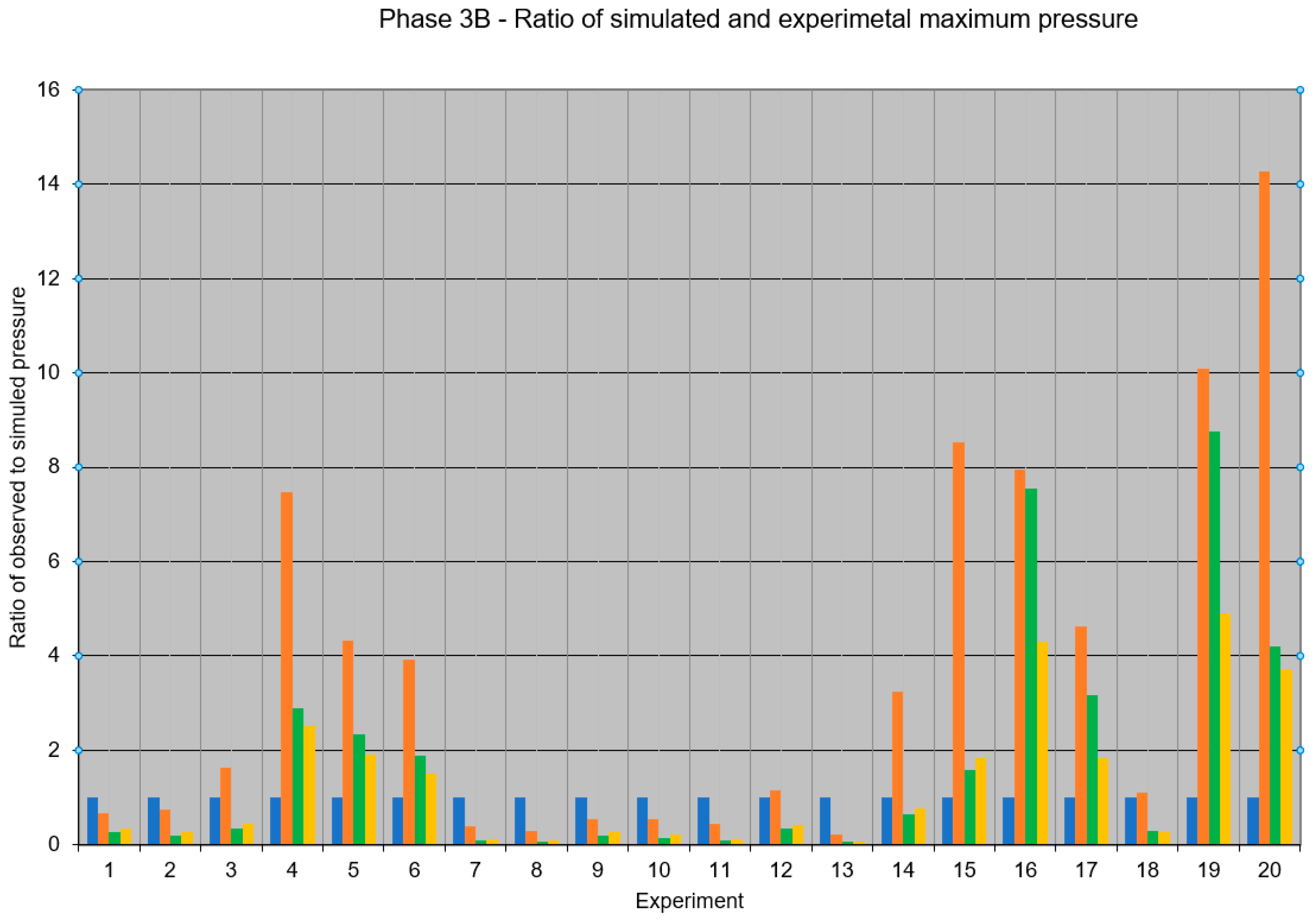
Figure 5.
(top): A figure showing a comparison of calculated maximum overpressure with measurement (reproduced from [3], and Figure 5 (bottom): the comparison of various ESC models against data (by the author) showing the ratio of model prediction with measured values. The number on the x-axis represents the test number in the experiment. The blue bar in the bottom figure is a reference showing the perfect agreement position of 1. Each colour refers to one ESC model; the exact ESC model is not important here. Both of these figures are confusing for the purpose of comparing model performance. The purpose of showing these two figures is to illustrate the difficulties in extracting overall biases and variance for various models.


Figure 6.
An MV diagram summarising the performance of the ‘direct dispersion-explosion simulations’ using FLACS. No ESC was assumed. Non-homogeneous flammable gas clouds were calculated and used directly as input to explosion simulations. Results from [3] in crosses and the Phase 3B reports [17] in hollow squares. Note about legend: a line is added to the start of a new symbol to allow its easy identification.

Figure 7.
Results of direct dispersion–explosion simulation using three grid sizes from the Blast and Fire for Topside Structure joint industry (BFTSS) Phase 3B project report. Grid size refers to grids outside the local refinement region round the release source. Note about legend: a line is added to the start of a new symbol to allow its easy identification.

Figure 8.
MV diagram showing performance of the Q9 model based on work carried out towards the Tam 2008 paper. The solid circles show results in which Q9 volumes were derived directly from experimental data (published in [2]). The crosses are results in which Q9 volumes are placed near the edge of the module. The variance of the blue cross is so large that it is outside the boundary of this figure. Note about legend: a line is added to the start of a new symbol to allow its easy identification.

Figure 9.
MV diagram showing the results using two grid sizes (0.5 m and 0.25 m) using current explosion risk assessment (ERA) methodology.
Figure 9.
MV diagram showing the results using two grid sizes (0.5 m and 0.25 m) using current explosion risk assessment (ERA) methodology.

Figure 10.
Exceedance curve showing cumulative frequencies for overpressures on a structural wall of a living quarter taken from A design study of an offshore production facility. These curves were derived from ESC model: Q9 and ∆FL (concentration between upper and lower flammability limits, this is labelled as “LFL-UFL”) in the legend).

Figure 11.
Cloud size vs. time profiles for Q9 clouds (taken from [3]). They show characteristic flammable cloud volume variation with time.
Figure 11.
Cloud size vs. time profiles for Q9 clouds (taken from [3]). They show characteristic flammable cloud volume variation with time.

Figure 12.
Calculated evolution of ESC volumes from experimental data for two ESC models: Q0 and Q5. This shows the sensitivity of the ESC model on maximum flammable cloud volumes and their evolution with time (taken from [17]).
Figure 12.
Calculated evolution of ESC volumes from experimental data for two ESC models: Q0 and Q5. This shows the sensitivity of the ESC model on maximum flammable cloud volumes and their evolution with time (taken from [17]).

Figure 13.
Comparison of predicted and observed maximum overpressures for all transducers in Test 17 in the Phase 3B JIP. The predicted values were calculated from FLACS using Q9 ESC and a grid size of 0.25 m.
Figure 13.
Comparison of predicted and observed maximum overpressures for all transducers in Test 17 in the Phase 3B JIP. The predicted values were calculated from FLACS using Q9 ESC and a grid size of 0.25 m.


Table 1.
Geometric Mean and Variance: direct dispersion–explosion simulations.
| Source | Hansen et al., 2013 [3] | Phase 3B Report [17] | ||
|---|---|---|---|---|
| MG | VG | MG | VG | |
| All | 0.73 | 12.2 | 0.68 | 11.7 |
| C1 only | 0.38 | 3.50 | 0.46 | 2.73 |
| C2 only | 1.17 | 26.5 | 1.10 | 63.6 |
Based on 0.5 m control volume.
Table 2.
Geometric Mean and Variance: direct dispersion–explosion simulations as a function of grid sizes. Results taken from the Phase 3B joint industry project (JIP) [17]. The results are based on maximum overpressure within the module (in experiments and in simulations).
Table 2.
Geometric Mean and Variance: direct dispersion–explosion simulations as a function of grid sizes. Results taken from the Phase 3B joint industry project (JIP) [17]. The results are based on maximum overpressure within the module (in experiments and in simulations).
| Grid Sizes | 0.5 m | 1 m | 1.33 m | |||
|---|---|---|---|---|---|---|
| MG | VG | MG | VG | MG | VG | |
| All | 0.68 | 11.7 | 0.54 | 18 | 0.30 | 32 |
| C1 only | 0.46 | 2.73 | 0.34 | 15 | 0.21 | 25 |
| C2 only | 1.10 | 63.6 | 1.0 | 22 | 0.45 | 42 |
Table 3.
Cloud located at locations conducive to generating high overpressures: Geometric Mean and Variance. Maximum P column taken from [2].
Table 3.
Cloud located at locations conducive to generating high overpressures: Geometric Mean and Variance. Maximum P column taken from [2].
| Maximum P | Average P | |||
|---|---|---|---|---|
| MG | VG | MG | VG | |
| All | 1.0 | 4.6 | 0.9 | 3.7 |
| C1 only | 0.7 | 1.6 | 0.7 | 1.7 |
| C2 only | 1.7 | 23 | 1.6 | 12 |
Table 4.
Geometric means and variance: Q9 Cloud volumes calculated by FLACS was used as an input to explosion simulations.
Table 4.
Geometric means and variance: Q9 Cloud volumes calculated by FLACS was used as an input to explosion simulations.
| Grid Size—0.5 m | Grid Size—0.25 m | |||
|---|---|---|---|---|
| MG | VG | MG | VG | |
| All | 0.6 | 13.7 | 0.6 | 7.5 |
| C1 only | 0.3 | 14.3 | 0.4 | 7.7 |
| C2 only | 1.5 | 12.7 | 1.2 | 7.2 |
Publisher’s Note: MDPI stays neutral with regard to jurisdictional claims in published maps and institutional affiliations. |
© 2021 by the authors. Licensee MDPI, Basel, Switzerland. This article is an open access article distributed under the terms and conditions of the Creative Commons Attribution (CC BY) license (https://creativecommons.org/licenses/by/4.0/).
Share and Cite
MDPI and ACS Style
Tam, V.H.Y.; Tan, F.; Savvides, C. A Critical Review of the Equivalent Stoichiometric Cloud Model Q9 in Gas Explosion Modelling. Eng 2021, 2, 156-180. https://0-doi-org.brum.beds.ac.uk/10.3390/eng2020011
AMA Style
Tam VHY, Tan F, Savvides C. A Critical Review of the Equivalent Stoichiometric Cloud Model Q9 in Gas Explosion Modelling. Eng. 2021; 2(2):156-180. https://0-doi-org.brum.beds.ac.uk/10.3390/eng2020011
Chicago/Turabian StyleTam, Vincent H. Y., Felicia Tan, and Chris Savvides. 2021. "A Critical Review of the Equivalent Stoichiometric Cloud Model Q9 in Gas Explosion Modelling" Eng 2, no. 2: 156-180. https://0-doi-org.brum.beds.ac.uk/10.3390/eng2020011