
Elevated LNG Vapour Dispersion—Effects of Topography, Obstruction and Phase Change


1
BP, I&E Engineering, Sunbury on Thames, London TW16 7LN, UK
2
School of Engineering, Warwick University, Coventry CV4 7AL, UK
*
Author to whom correspondence should be addressed.
†
Retired, formerly BP, no email address.
Eng 2021, 2(2), 249-266; https://0-doi-org.brum.beds.ac.uk/10.3390/eng2020016
Submission received: 6 April 2021
/
Revised: 10 June 2021
/
Accepted: 11 June 2021
/
Published: 15 June 2021
(This article belongs to the Special Issue Valorization of Material Wastes for Environmental, Energetic and Biomedical Applications)
Abstract
:The dispersion of vapour of liquefied natural gas (LNG) is generally assumed to be from a liquid spill on the ground in hazard and risk analysis. However, this cold vapour could be discharged at height through cold venting. While there is similarity to the situation where a heavier-than-air gas, e.g., CO2, is discharged through tall vent stacks, LNG vapour is cold and induces phase change of ambient moisture leading to changes in the thermodynamics as the vapour disperses. A recent unplanned cold venting of LNG vapour event due to failure of a pilot, provided valuable data for further analysis. This event was studied using CFD under steady-state conditions and incorporating the effect of thermodynamics due to phase change of atmospheric moisture. As the vast majority of processing plants do not reside on flat planes, the effect of surrounding topography was also investigated. This case study highlighted that integral dispersion model was not applicable as key assumptions used to derive the models were violated and suggested guidance and methodologies appropriate for modelling cold vent and flame out situations for elevated vents.
1. Introduction
It is common to use the integral jet dispersion model to assess hazard distances of the discharge of flammable gases for elevated discharges, such as a tall vent stack or from an elevated flare during cold venting. The use of the integral jet dispersion model assumes that the discharge occurs in uniform ambient wind field with no orographic effect and there are no heat sources or sinks involved in the thermodynamics in the dispersion processes. In many real situations, these assumptions are not valid. In this paper, a case study is described, which illustrates situations where these assumptions are not valid and the consequences of the outcome of assessment.
This paper illustrates the concerns of dispersion of a very cold momentum gas jet from height. The scenario involved the discharge of liquefied natural gas (LNG) vapour at speed and at a height through an elevated vent stack. One of the purposes of a vent stack is for the safe dispersal of routine or emergency release of flammable gases. Some vent stacks have a pilot light to allow the flaring of these gases. In the event of the failure or absence of a pilot light, stack design ensures that the emitted gas would not be hazardous to people or facilities downwind. By virtue of its height and location, vent or flare stacks, in general, are designed to be inherently safe: disperse harmlessly in the atmosphere and not posing flammable or toxic hazard to personnel or the process facilities. This is done via a few methods such as locating the stack at a far enough distance from the facility, a high enough stack or optimal diameter of stack to allow high velocity venting. This ensures turbulence has sufficient time and intensity to dilute the discharged gas to harmless concentrations.
1.1. Common LNG Dispersion Scenarios
It is assumed generally, in hazard and risk analysis, that a spill of LNG is on the ground or on the water or sea. This covers scenarios such as a spill from low level pipework, leaks from storage tanks and spills into the sea during loading and unloading from LNG tankers. The physics involved is relatively simple to conceptualise and model.
The vast majority of consequence analysis for risk analysis purposes use evaporation-and-boiling model in conjunction with integral dense gas dispersion model for these situations. The most common model in used is dense gas dispersion model based on work by Haven [1] for spills on land/sea/water.
1.2. A Less Common Scenario
In the less common scenario, cold LNG vapour is vented in an elevated position, as mentioned earlier. This is usually addressed at the design of the vent stack/flare, the approach is to use an integral atmospheric jet dispersion model such as the one based on Ooms [2]. Integral atmospheric jet dispersion models are widely used to estimate flammable hazard distances, for design (e.g., zoning of hazard zones, in the design of cold vents to define vent heights required for safe dispersal, etc.) and for risk assessment (e.g., small to large leaks in hydrocarbon process areas). Flammable hazard distances are often defined by the distances to half of the lower flammability limits (LFL) (or sometime to LFL) of the released gas mixtures in air, and they are often calculated accordingly.
Integral atmospheric jet dispersion models are simple and can be easily solved using office computers. However, these models contain many assumptions some of which are physically unrealistic for LNG vapour dispersion assessment.
1.3. Assumptions
Current integral jet dispersion models are based on the elevated dispersion model developed in the early 1970s to assess effects of pollutants from tall stacks for environmental impact assessment. Coal fired power stations were common. Many of them were located close to or within heavily populated cities (e.g., the Battersea power station in London). The prime application of the model was the assessment of the impact of the pollutant, particularly sulphur, on air quality on communities immediate downwind of the chimney. A jet dispersion model (also called high momentum dispersion model, or elevated plume model) describes the dispersion of a gas discharged at velocities, significantly higher than ambient wind velocities.
Integral atmospheric jet dispersion models are usually embedded in commercially available consequence analysis packages such as PHAST by DNVGL for the oil/gas/petrochemical industry. Some major international companies and consultants have their own in-house package, e.g., CIRRUS in BP or FRED in Shell. The most widely used commercial packages have become the ‘industry standard’ and their use is sometime written into technical guidance and practices (e.g., [3]).
These integral models assume uniform conditions to simplify the physics and mathematics involved. The key assumptions are: (i) constant wind velocities, (ii) constant and uniform turbulence that implies perfectly flat terrain and no large buildings or equipment close by upstream and downstream and (iii) there is no mass or energy source or sinks, which implies there is no phase change. In practice all the above assumptions are violated for the dispersion of cold LNG vapour.
1.4. Objectives
The objectives of this analysis were to model using computational fluid dynamics (CFD) and quantify the effects of the common assumptions on conditions typically found on an LNG installation, such as topography and cold temperature of the LNG vapour, and to compare calculated results with data obtained from a recent unplanned cold venting of LNG vapour event due to failure of a pilot.
1.5. Cold Venting Incident—A Case Study
This incident occurred during the night. There was a planned maintenance that required LNG to be discharged to flare. On this occasion, the pilot failed. This led to a large amount of cold boil-off LNG vapour (estimated to be about 200 tonne) vented from a 35 m tall flare stack over a 5 h period. Cold venting can be part of planned actions. However, unintended incidents involving cold venting are often the results of the flare pilot systems failure or being isolated under specific known operational conditions. In this incident, the pilot system was inactive and the extinguished pilot alarms were left unnoticed by the facility control room operator. This incident resulted in the triggering of the facility gas detection system, specifically, line-of-sight detectors located in several locations at the processing facility to the south and downwind of the stack. The north of the facility (closest point to the stack) is situated approximately 800 m away from the flare. The gas concentration measurements in the region of interest (gas detectors that were activated at the facility during the incident were situated at the north sector of the facility) were logged and were used in this modelling analysis. The gas concentration was recorded in terms of concentration in unit of lower flammability limit integrated over distance in metre (LFL m) and it was of >3 LFL m over a distance of 13.5 m (average concentration of >0.2 LFL/m over this distance) with these values corresponded to average concentrations over a period of 30 s. The corresponding LFL reading during the incident was 2–15% LFL. It should be noted that the low set point of these line-of-sight (LOS) gas detectors was 0.2 LFL m or 20% LFL for 1 m coverage. Point detectors on the facility had set points of 20% LFL. Thus, it was possible to trigger the line-of-sight detectors without triggering point detectors, and vice versa.
2. Methodology
2.1. The Facilities
Figure 1 is a schematic layout of the LNG facility chosen for this study. The figure shows the location of the vent stack and topographical features. This facility is in the tropics with high ambient humidity throughout the year. Alongside detailed information on topography and plant layout, LNG vapour concentration reading from gas detectors were available for one time period from a recent unplanned cold venting event. The atmospheric conditions at the facility during the incident were available from nearby weather stations and used in the modelling: (i) air temperature during the incident was about 33 °C, (ii) relative humidity of 90%, (iii) wind speed was constant at 2 m/s at 10 m height and (iv) wind was blowing from the sea carrying the release gases towards the area of interest.
2.2. Computational Methods
As mentioned above, integral models were not adequate for this study. This is discussed in detail later. Integral models were used in the initial assessment of this incident and were found to be inadequate in explaining the event.
The computational fluid dynamics (CFD) code STARCCM+ was used for this study. The geometric model was constructed using the CAD data of the plant. Outside the confines of the CAD model, other generic data were used to include the vent stack, terrain, the two storage tanks explicitly. The dimensions and locations of these additional blockages were matched closely to the actual facility and used to calculate the drag source term and capture accurately their impact on the LNG dispersion.
2.2.1. Domain
The CFD calculation domain encompassed an area of 5 km2. This area took into account sufficient distance upstream, for realistic flow establishment at the vent stack, and downstream to beyond the concentration of interest.
2.2.2. Gridding
Owing to the large area being considered, the number of grid cells was minimized using multi-block grid refinement techniques. Local grid refinements were used to ensure that the plume shape and behaviour was accurately captured (see Figure 2). In total, 8 million grid cells were needed, comprising of a mixture of prisms, hexahedra and polyhedral.
2.2.3. Subgrid
For the purpose of this study, resolving the entire LNG plant was not necessary for the CFD dispersion analysis. Although the plant is over half a kilometre away, the blockages created by plant equipment and supporting structures would have an impact on the plume behaviour and on the ground-level concentrations near the area of interest. To resolve these items explicitly would render a vast increase in grid cell number and computer runtime. The two large tanks and large pieces of equipment were explicitly resolved. The effect of all process equipment, structures and pipework in the process area were represented in a ‘subgrid scale’ manner, i.e., their ‘blockage’ effects on the flow were modelled through local drag terms in the momentum equations derived from the properties of items from the CAD model for each grid cells. The drag terms were directional, e.g., for a subgrid scale pipe, there was negligible drag force along its length. Figure 3 presents the locations where subgrid scale modelling was used.
2.2.4. Boundary Conditions
The boundary conditions used in the CFD modelling included vertical inlet wind profiles for a neutral atmospheric stability class, the appropriate velocity and turbulence factors (kinetic energy and dissipation rate). For the outlet of the computational domain, flow split outlet conditions was assumed.
2.3. Effect of Water Moisture
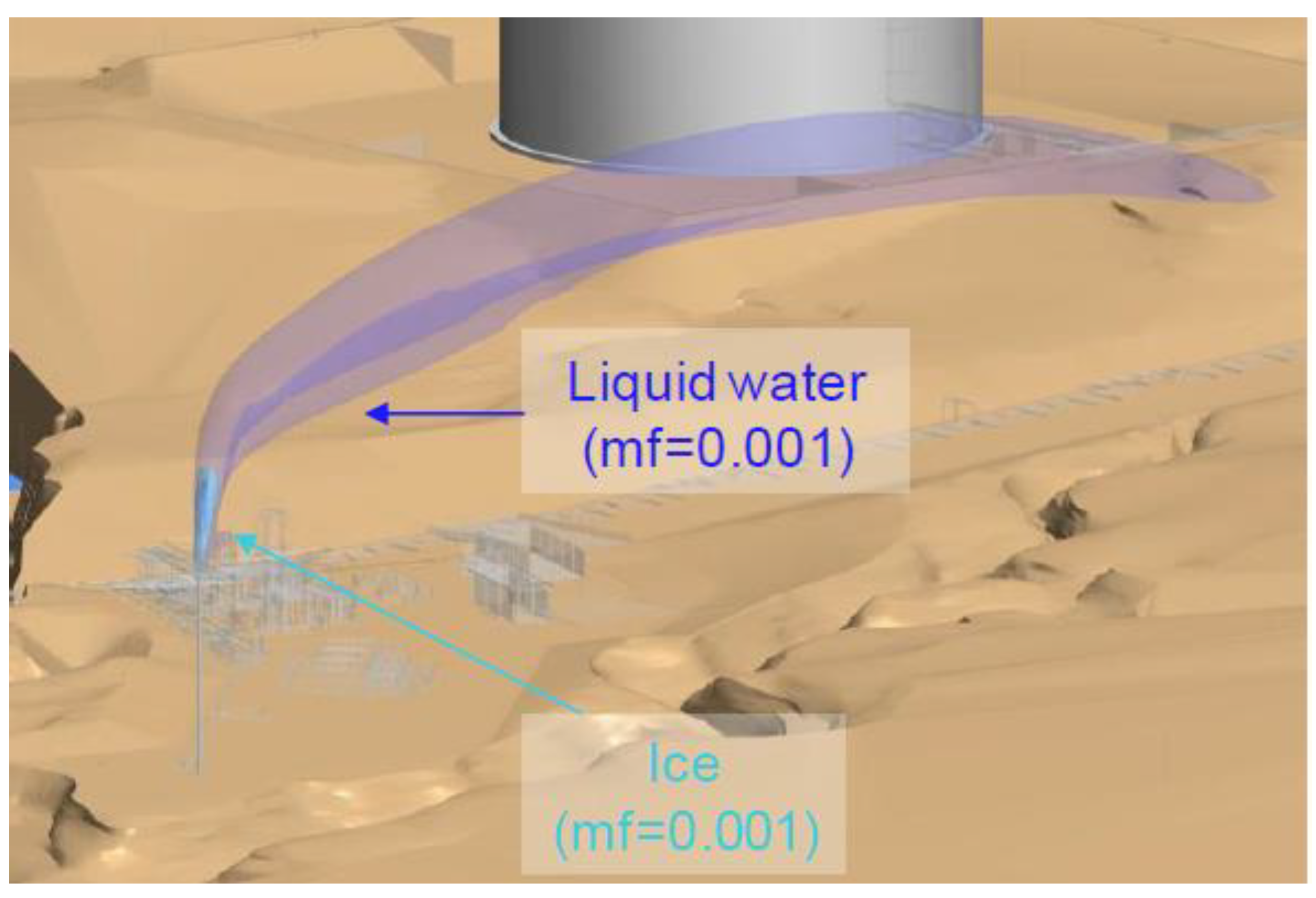
The cold LNG vapour was at −161 °C, well below the freezing point of water. Moisture in the air would freeze forming a particulate suspension, increasing the effective density of the plume. This affected its behaviour and thus the concentration levels near the process areas, which were of interest. As well as dispersion, freezing, condensation, melting and evaporation of ambient air moisture were also modelled. It was also assumed that the various phases of water be treated as gaseous components with the appropriate composite molecular weight. This was to ensure that all the phases had the same velocity and temperature in each computational cell and that the density effects of the liquid and solid water were accounted for and affected the plume behaviour. Mass fraction of liquid water and ice that was present in each cell was small enough to be treated as dense gases. The mass and energy transfers between the phases in the entire CFD model based on local flow characteristics. We encountered numerical stability problems on these transfers and instigated numerical measures to control it. Figure 4 presents the plume iso-surfaces of ice and liquid water for a mass fraction of 0.001. For this study, relative humidity was assumed to be 90%, corresponding to a facility located by the sea in the tropics.
2.4. Topographical Effect
The bottom boundary of the calculation domain followed the contour of the terrain at the facility. The following conditions were applied: (i) no slip, (ii) rough wall boundary condition with an appropriate roughness value to account for the terrain vegetation distribution and (iii) adiabatic thermal boundary.
2.5. Steady State
As with integral models, this study focused on a steady-state solution. The total calculated flammable vented gas volume was used as an indicator for steady state (or computational convergence). Results were taken only when this has stabilised for a continuous and sufficient number of timesteps (>1000).
2.6. Venting Rates
Four venting rates were used in the study to represent various stages of the venting incident: 16 kg/s, 25 kg/s, 30 kg/s and 45 kg/s. The LNG vapour was assumed to have the physical properties of methane at a molecular weight of 17.2 and at a temperature of −161 °C, discharged at the top of the 20-inch diameter stack at height of 35 m above local ground level.
2.7. Wind Directions
The normal practice would be to align the wind direction towards the area of interest, in this case, the nearest point in the process plant. It was the hazardous and occupied area with potential for ignition. Four other wind directions about this direct alignment direction were also investigated and these are shown in Figure 5. The 5 wind directions assessed were representing wind blowing from 316° N to 338° N. These directions were chosen to be at or near the point where the plume could be obstructed or deflected by the 2 large storage tanks situated south of the flare stack but north of the process area. These storage tanks have measurable impact on the dispersion and impact on ground level gas concentration in the process area downwind.
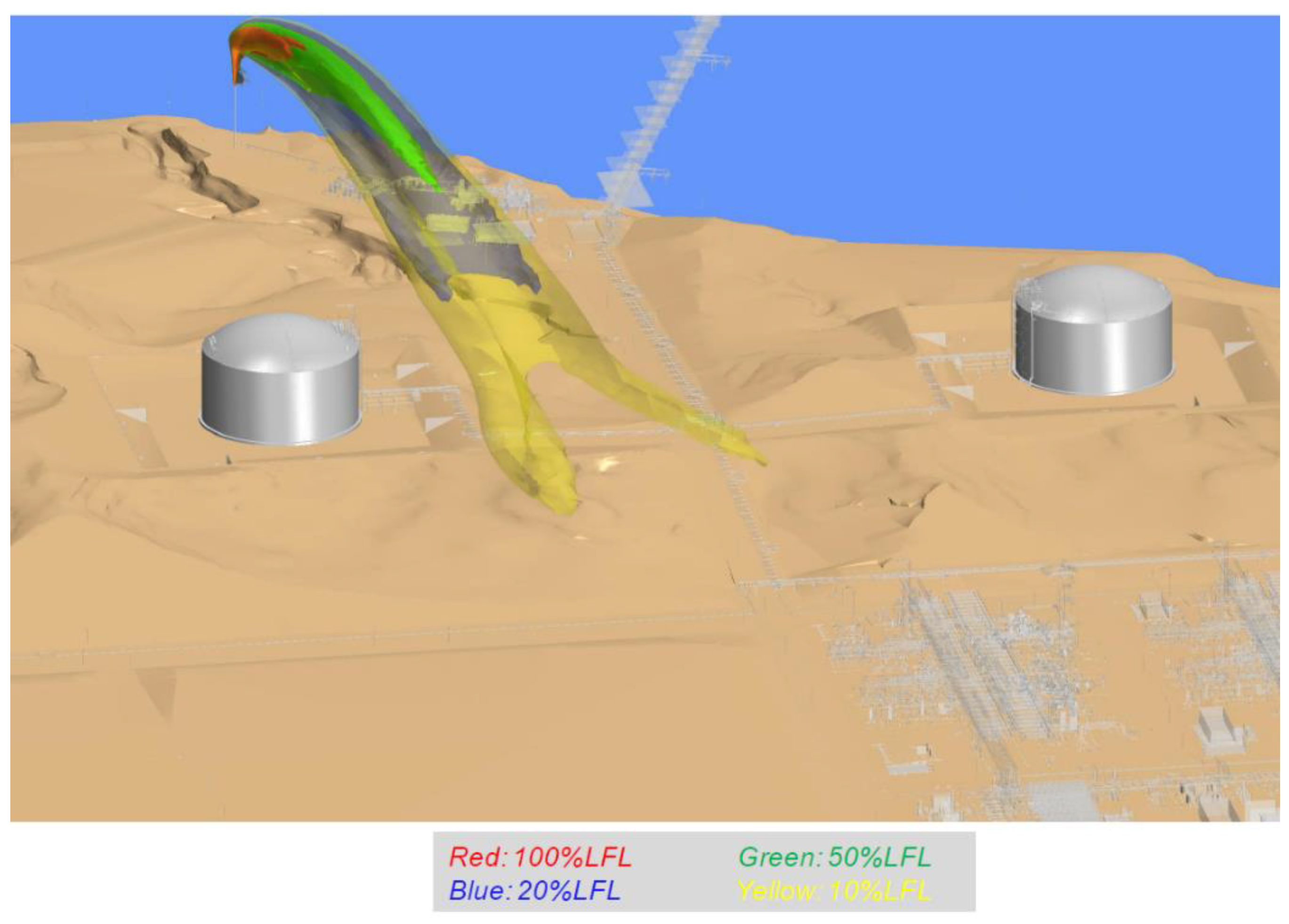
3. Results
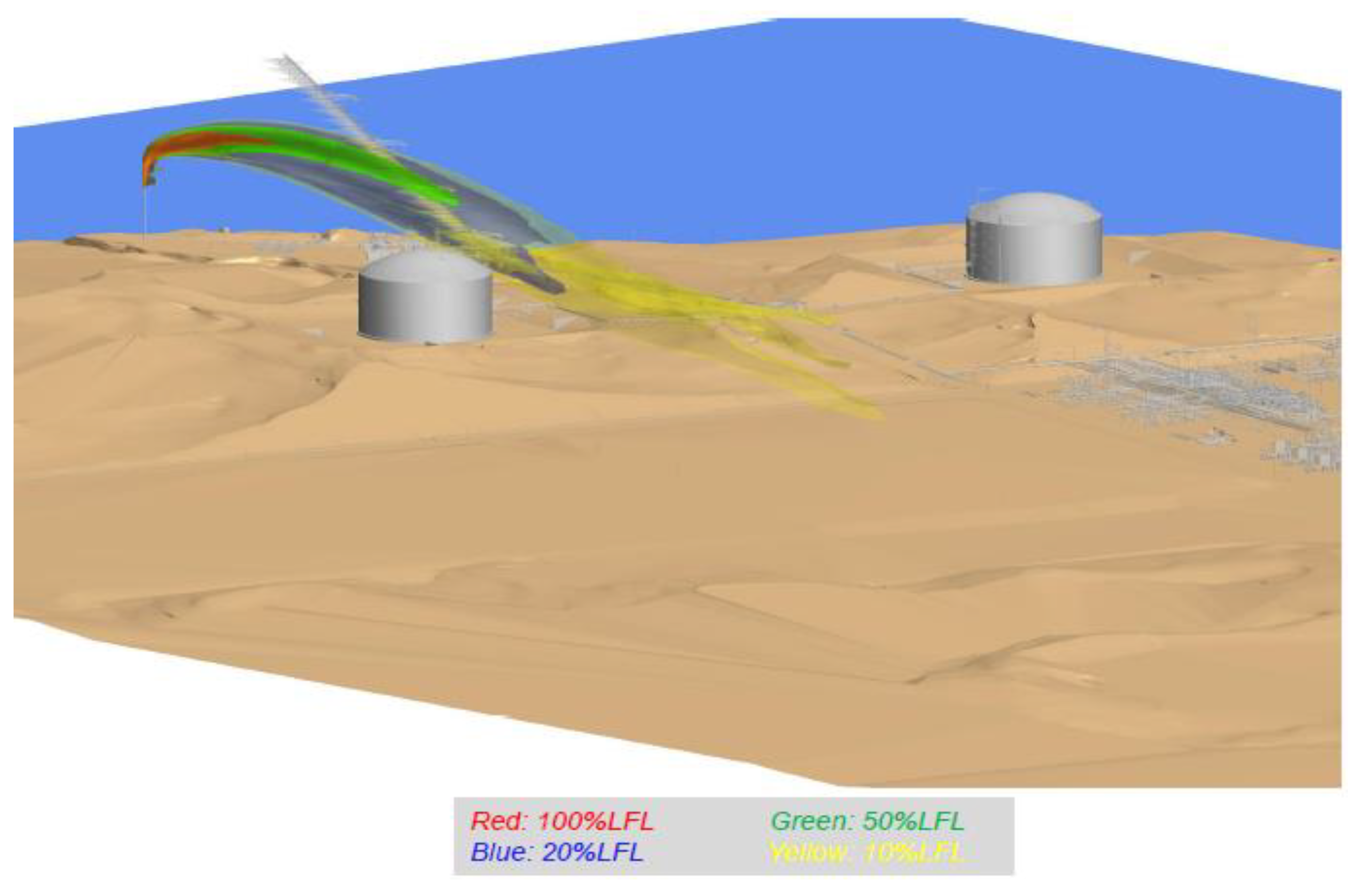
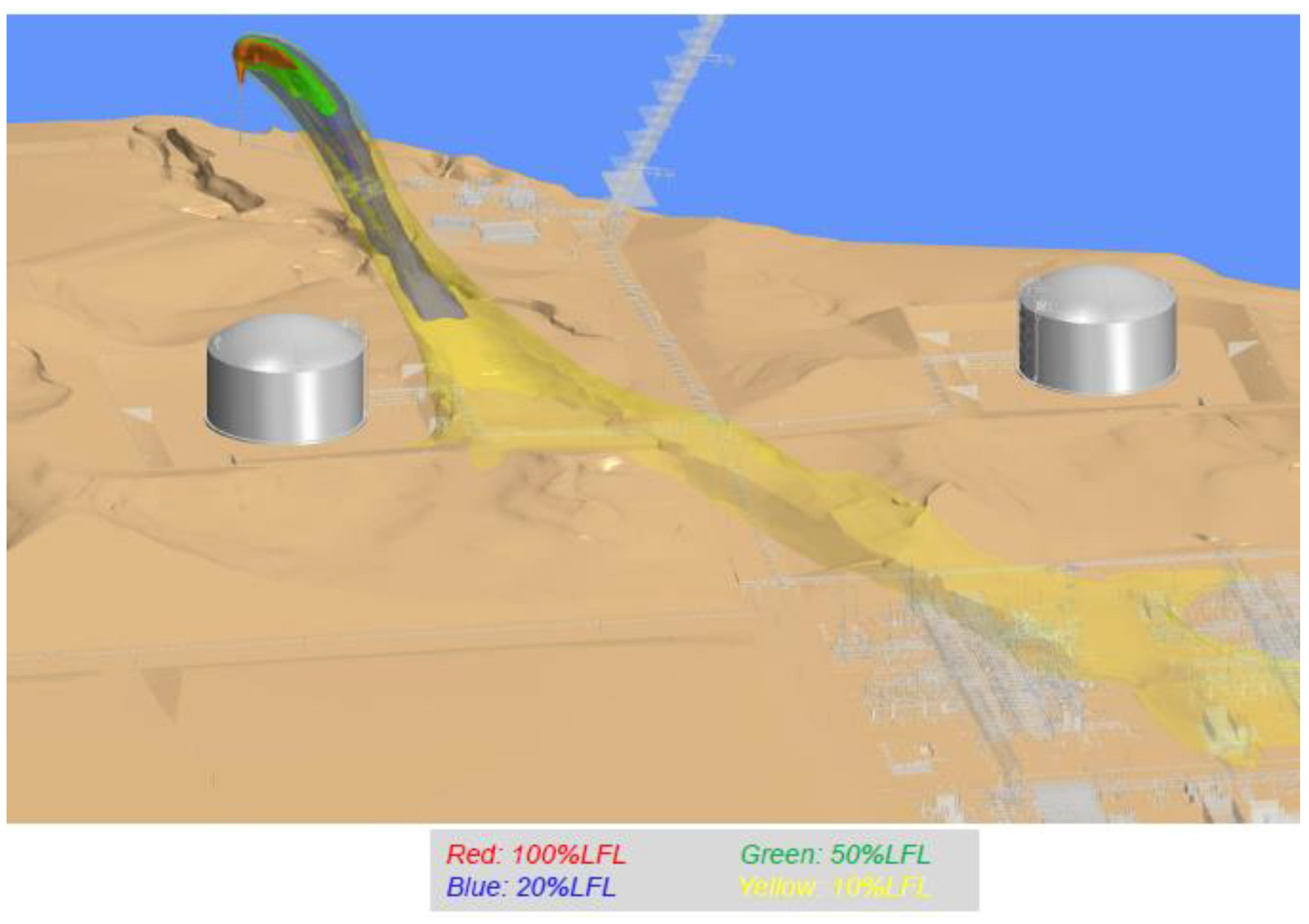
Figure 6 represents a general 3D plot of the plume dispersing in the direction towards the process train. The colour of the iso-surfaces represents different levels of LFL concentration in the plume. As expected, the highest gas concentration would be immediate at the vent outlet and the lowest gas concentration would be at the farthest distance from the vent. The plume rose, levelled off and after a distance, descended onto the ground along which the plume continued to disperse. A summary of results is given in Table 1, which shows the effect of release rates, wind directions and wind speeds.
In general, the results showed that the vent stack was sufficient to disperse the LNG vapour sufficiently that it did not pose a flammable hazard on the plant, even at a high vent rate of 45 kg/s. The ground level concentration would have been zero using integral jet dispersion model. However, the focus of this study was less focused on the design adequateness but rather to explore factors that could have significant impact on the dispersion behaviour.
There were results that showed trends that were consistent with current common understanding of dispersion; the increase in target concentration occurred as release rate also increased (Cases 1, 1a and 1b).
There were also contrary results too. Concentration at the target area increased as wind direction deviated away from that which directly aligned with the vent and the target area. This is an example of effects of interaction between the wind field and terrain and the two large storage tanks.
3.1. Variation of Vent Rates
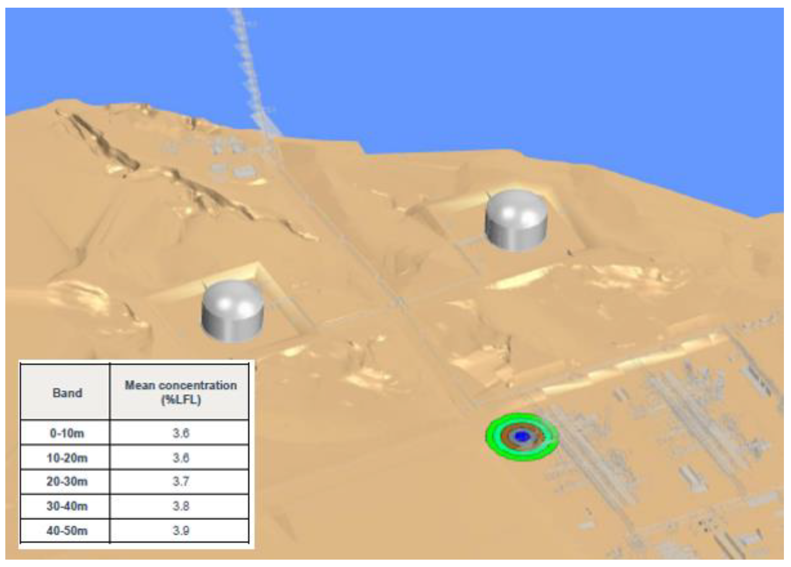
This section summarises the results of Cases 1, 1a and 1b where the vent rates ranged from 25 to 45 kg/s at a constant wind speed of 2 m/s from direction 1. Figure 7 represents the plume extent from Case 1, venting rate of 25 kg/s with 2 m/s wind from direction 1. The plume could be seen to meander downwards and in between both large storage tanks. The mean concentrations on the ground level were also captured. In order to compare gas measurements obtained during the incident with the CFD prediction, mean concentrations were also obtained from the modelling in terms of five concentric 10 m bands close to the position where the field measurements were obtained. The predicted values were about 3.7% LFL as compared to the minimum of 2% LFL measured on site (see Figure 8).
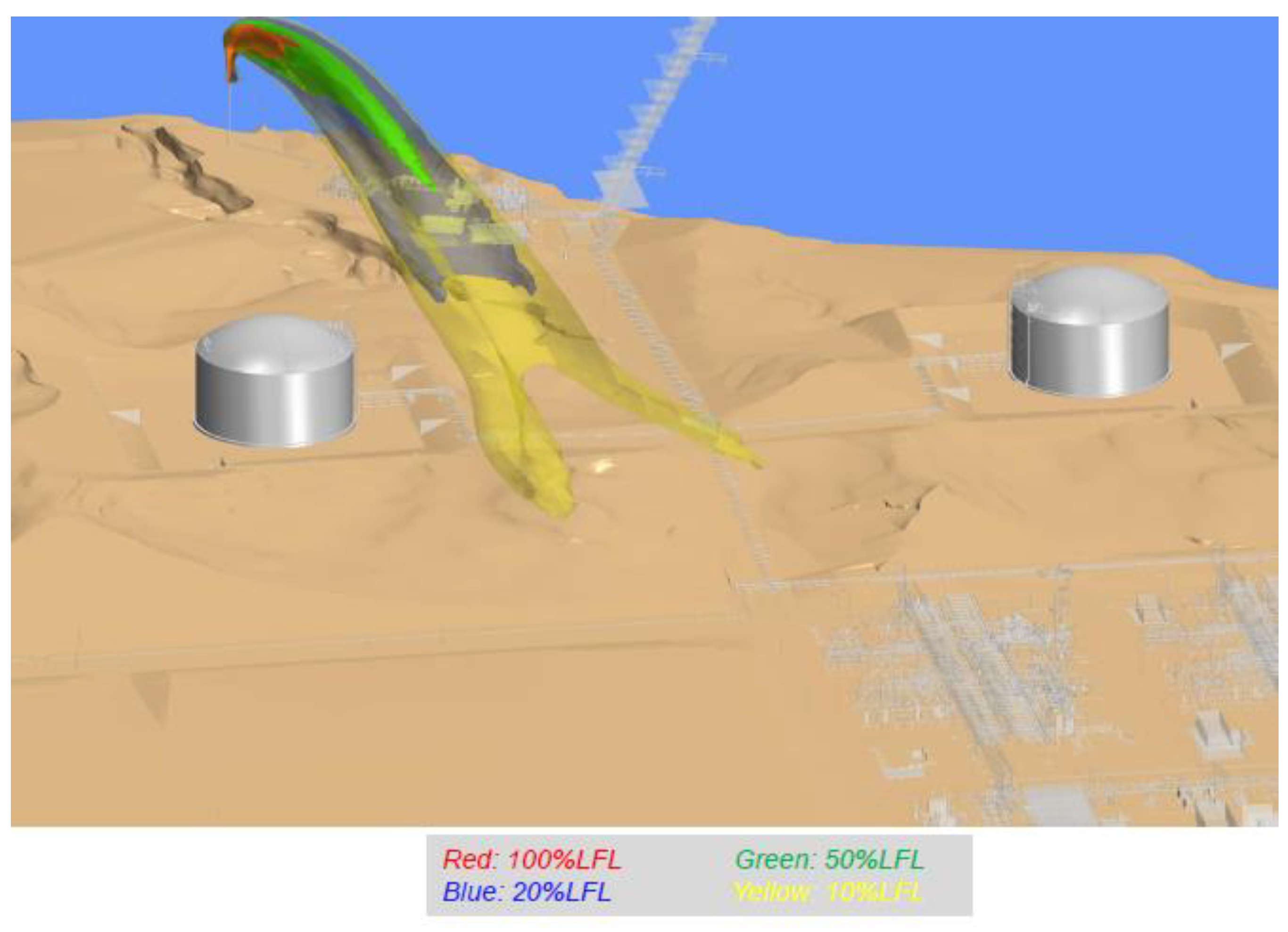
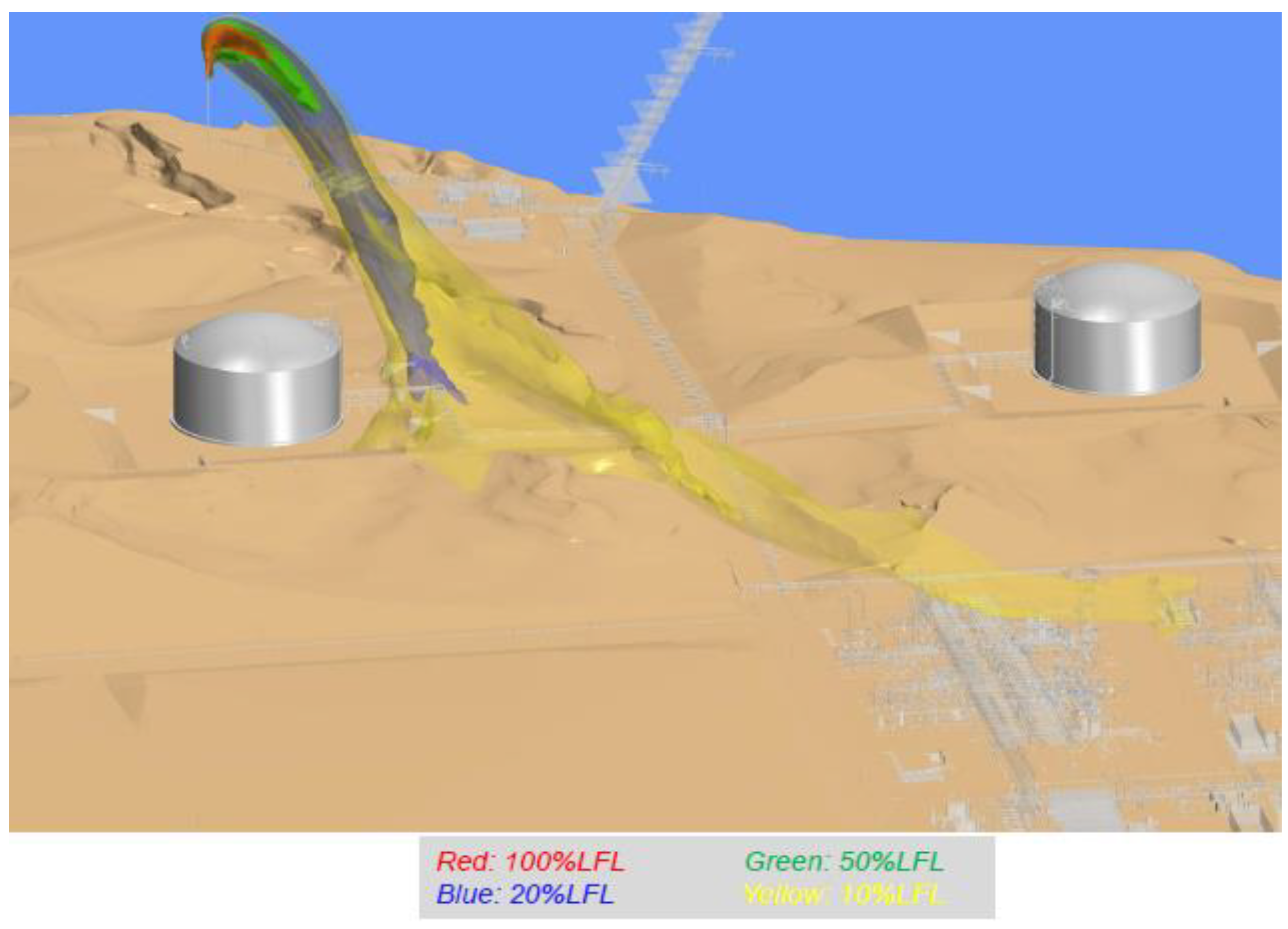
Case 1a is for the high release rate case of 30 kg/s, the effect of the topography could be seen with the plume splitting up into two, close to the vent exit and then descending onto the ground at two locations. This is shown clearly in Figure 9.
Again, mean concentrations near gas measurements were represented in five concentric 10 m bands. The predicted values were around 4% LFL as compared to the minimum of 2% LFL measured on site.
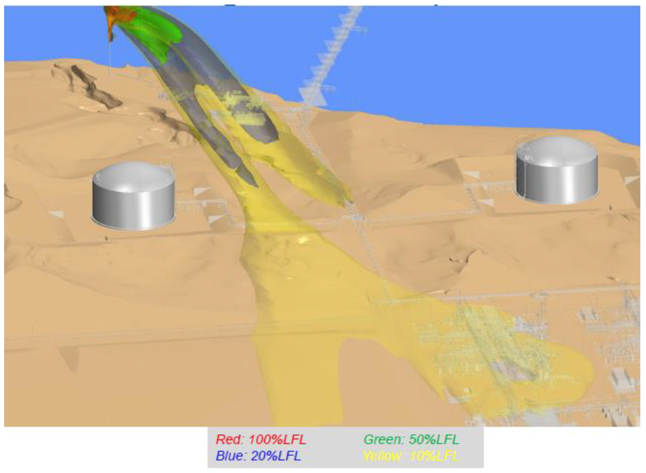
Figure 10 show the plume extent for Case 1b, the largest flowrate modelled of 45 kg/s and the ground concentration distribution at the process area. At this larger flowrate, it could be observed that a larger gas cloud reached the process area and touched down at two separate locations. Again, mean concentrations were also monitored at five concentric 10 m bands close to the position where gas measurements were obtained, and the predicted values were around 12.5% LFL compared to the minimum of 2% LFL measured on site.
In general, ground level concentrations tended to increase in the process area with increasing vent rate. Low vent rate could lead to earlier touchdown of plume as observed in the iso-surfaces above. Venting rate of 25 kg/s produced a higher ground level concentration closer to the storage tanks than higher vent rates. This is summarised in Figure 11, which shows the ground level concentration distribution and touchdown locations for all 3 vent rates at 2 m/s from direction 1. The maximum ground level concentration at any location on the facility was about 10% LFL, which was below the facility point detectors low trigger set point of 20% LFL. The concentration at the location of interest and LOS detectors were estimated to be about 4% LFL and whilst this concentration was lower, it could trigger the LOS detectors. Note that during the incident, an equivalent reading of 2 to 15% LFL was captured by the LOS detectors.
3.2. Variation of Wind Directions
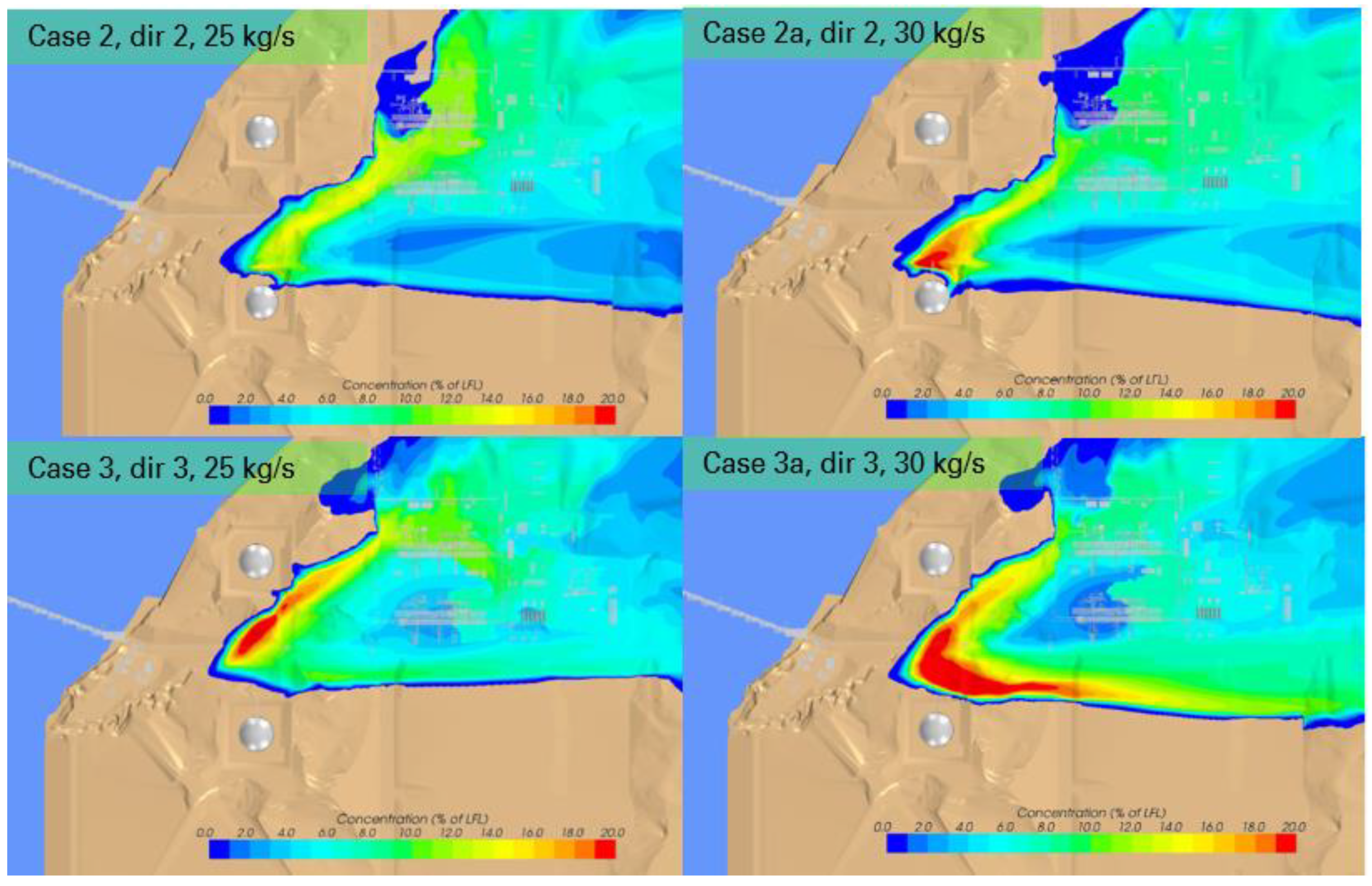
Wind direction 2 was modelled to be slightly farther clockwise of wind direction 1, going towards the west of the facility. Figure 12 shows the plume extent for Case 2, 25 kg/s release under 2 m/s wind. The plume was observed to potentially encroach on the process areas. This was in contrast with Case 1 (see Figure 7) where the plume dispersed more towards the east side of the facility. The mean concentrations monitored in 5 concentric 10 m bands close to the location of the LOS detectors were predicted to be about 5.5% LFL as compared to the minimum of 2% LFL measured on site.
Vent rate of 30 kg/s was also modelled under the same wind conditions. Figure 13 shows the extent of the plume for Case 2a where the plume concentration of 10% LFL covered a smaller area of the process facility as compared to the plume of 25 kg/s. Due to the higher flowrate, the same wind speed was less effective in dispersing the gas cloud, i.e., the higher concentration band of 20% LFL for Case 2a can be seen to be larger than Case 2. The mean concentration on the ground in the concentric bands were observed to be about 6.3% LFL.
Wind direction 3, anticlockwise of direction 1, going towards the east of the facility, was also modelled for the same flowrates of 25 and 30 kg/s. The plumes extended more towards to the east of the facility therefore led to lower mean ground concentration at the area of interest. The concentric bands measured 3.3 and 3% LFL for 25 and 30 kg/s releases, respectively. This was lower in comparison to the concentrations of 5.5 and 6.3% LFL for direction 2. See Figure 14 for a summary of ground level concentration for wind directions 2 and 3.
Wind directions 4 and 5 were also modelled for the same venting flowrate of 16 kg/s. The wind speeds were varied between 3.9 m/s and 3 m/s (see Figure 15). The ground concentration plots showed that for the higher wind speeds of 3.9 m/s, the plume did not reach the area of interest for wind direction 4 (Case 4) and reached the end section of the first LNG train for wind direction 5 (Case 6). However, as the wind speed decreased (Case 5), the plume touched the ground earlier and mean concentrations of about 3.7% LFL were observed near the LNG trains.
4. Discussions
The results of the CFD analysis showed that the likelihood of the plume touching down did not increase with vent rate, which was counterintuitive. As the release rate from the vent decreased, the concentration at the target sensor increased. This was the condition that encouraged the gas plume to touch down early in low wind and low release rate conditions. At higher wind speed, the plume dispersed aloft sufficiently that it did not descend to ground. No ground level concentrations were detected.
4.1. Comparison with Measurements
Readings from the log of gas detectors indicated that the LNG plume had touched down. This aspect agreed with the CFD results here. The reading further indicated that the gas concentration was between 2% LFL and 15% LFL. The calculated figures fell within this range (Table 1).
4.2. CFD vs. Integral Model
Prior to carrying out this CFD study, analysis using integral dispersion models were used. This included a jet dispersion model for an elevated source and a dense gas dispersion model for a low momentum source. This was conducted immediately after the incident with time constraint and limited field data for comparison. However, as mentioned in the section above on model assumptions, the initial calculations using integral jet dispersion model showed that the LNG plume continued to rise after its release and remained aloft throughout. The calculated ground level concentration consequently was very low. When the heavy LNG vapour was assumed to descend to the ground and then dispersed, the calculated concentration level at the distance of the target area was about 30% to 40% LFL for a vent rate of between 20 and 40 kg/s (compared to 2% to 15% LFL gas detector readings).
These calculations showed that commonly used integral jet dispersion model underestimated the flammable hazards as it did not predict the descend of the plume. The dense gas model, by not accounting for the initial momentum mixing, over-estimated the flammable hazards. It was recognised that the integral model was not applicable in this situation because: (i) the topography was not flat as there was a hill between the vent and storage tanks; (ii) there were two large storage tank in the path of dispersed vapour, before the process area, thus the topography and equipment could drag the plume towards the ground; and (iii) the very cold temperature of the vented gas could have condensed moisture in the atmosphere increasing the effective density of the plume. These effects will be described further below. It is therefore, in situations like those described in this paper, advisable to use CFD analysis.
4.3. Moisture Effect
Moisture in the air could affect the plume dispersion at various stages of the plume. The condensation and freezing led to formation of ice particles and release of latent heat. As the plume entrained warmer air, ice melted and then evaporated, absorbing heat and cooling the plume in the process. The mean plume temperature along its trajectory deviated from that when there was no moisture. The evolution of different phases of moisture in the plume is shown in Figure 4.
It is common practice in dispersion calculations to ignore the effect of moisture in air [4,5]. An alternative simpler approach had been used. Rather than modelling the evolution of moisture during dispersion, a modifier of ambient air properties could be used instead [6].
In a recent CFD study on Burro and Coyote LNG spill tests carried out in deserts in the USA, the effects of moisture in air on dispersion behaviour was found to be significant [7]. At 5% relative humidity (RH), the difference in calculated concentration at a location for including or excluding moisture effect was relatively small (~10%). However, the difference quickly rose to about 30% at an RH of 22%.
4.4. Good Match with Visible Plume (Not a Reliable Measure of Flammable Plume Shape)
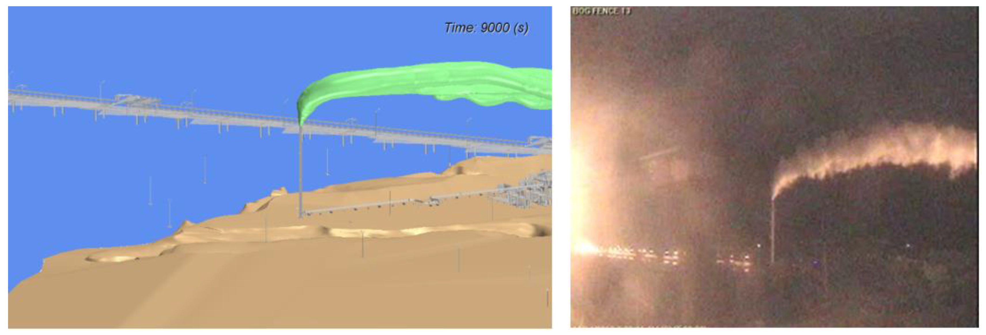
It was tempting to use the visible plume to inform oneself of the flammable hazard distances or predict position of the plume when it descended to the ground, or whether it would descend to the ground. As can be seen in Figure 16, the calculated plume shape matched well with the observed visible plume; however, it was difficult to deduce the complete plume trajectory based on visible plume information.
Furthermore, the visible plume was not a good indicator of flammable extent as it would be dependent on RH [8]. For the plume section that was aloft, it was the RH local to the plume which may vary with height and locations; it was highly unlikely to be the same as that measured on the ground.
4.5. Ground Effect
Topographic effect was very evident from the results. It altered the wind velocity field and its distribution in the entire calculation domain. This resulted in the splitting up of the plume leading to two touch-down points and meandering ground level plumes, the trajectories of which were determined by the ground contours and the wind field (see Figure 6). This was consistent with the long standing guidance for environmental assessment [9].
4.6. Effect of Storage Tanks
Large objects, such as storage tanks, had similar effect as topography, but the effects were local. These large objects could induce downdraft, dragging the plume downward, promoting earlier touchdown or increased ground level concentration. This effect could be seen in Case 4 and 5 of Figure 15 where higher concentrations of vented gas was observed at the upstream side of the large storage tanks.
4.7. Plume Touchdown Location
The location of plume touchdown would affect the location and size of the hazard zone. A higher ambient wind increased the distance of the touchdown zone, giving a higher gas concentration at ground level farther downstream of the facility, rather than the target of interest or locations closer to the vent stack (see Table 1). For example, at 3 m/s wind speed in direction 5, the ground level concentration at the target area is 3.7% LFL, this is reduced to 0 at a higher wind speed of 3.9 m/s.
As the above results show, touchdown locations depend on the complex interactions between wind speed, wind direction with topography and equipment.
4.8. Further Work
As environmental conditions and vent rates changed with time, the next step is to assess these effects. It was deemed possible that during the analysis that the range of wind speeds and directions could be larger than those suggested by steady-state conditions. This is the subject of a separate paper that is in preparation.
4.9. Other Scenarios
This study addressed scenario which was not routinely assessed. There are other scenarios where LNG vapour can be generated at height, and they are beginning to be studied. This included the EU funded project SafeLNG that considers the vapour generation and its dispersion following a release of LNG at height which might have occurred after the rupture of an LNG import or export pipework at the top of an LNG tank [10].
5. Conclusions
This paper describes a CFD study of cold venting of LNG vapour. The integral dispersion model was found to be inadequate as many of its assumptions are not met, e.g., perfectly flat terrain.
The cold vapour induced phase change of ambient moisture, leading to changes in the thermodynamics as the vapour dispersed. This affected the dispersion and trajectory of the plume, i.e., aloft time, distance, touch down location and local ground concentration.
Topography and equipment altered the wind velocity field in the entire calculation domain, e.g., storage tanks downstream of the vent produced downwash effects, dragging the plume aloft down towards the ground, promoting earlier touchdown or increasing ground level concentration.
The analysis also showed the effects of different release rates, wind directions and wind speeds. There were results which showed trends which were as expected, i.e., increase in target concentration as release rate increased, but also contrary to expectation, i.e., concentrations at target area increased as wind direction deviated away from that directly aligned with the vent and target areas.
The results from this analysis showed broadly good agreement with key observations.
Author Contributions
Conceptualization, V.H.Y.T.; methodology, F.T., V.H.Y.T. and C.S.; formal analysis, F.T., C.S.; investigation, F.T., V.H.Y.T., C.S.; resources, C.S., F.T.; data curation, F.T.; writing—original draft preparation, V.H.Y.T.; writing—review and editing, F.T., C.S.; supervision, V.H.Y.T.; project administration, V.H.Y.T. (Key: F.T.—Felicia Tan, V.H.Y.T.—Vincent H. Y. Tam, and C.S.—Chris Savvides). All authors have read and agreed to the published version of the manuscript.
Funding
This research received no external funding.
Institutional Review Board Statement
Not applicable.
Informed Consent Statement
Not applicable.
Data Availability Statement
Not applicable.
Acknowledgments
Authors would like to thank Christophe Mabilat (then Atkins UK) for the generation of results and figures in this paper.
Conflicts of Interest
The authors declare no conflict of interest.
Abbreviations
| CFD | Computational Fluid Dynamics |
| EU | European Union |
| LFL | Lower flammability limit |
| LOF | Line of Sight |
| LNG | Liquefied natural gas |
| RH | Relative humidity |
References
- Spicer, T.O.; Havens, J.A. Field test validation of the degadis model. J. Hazard. Mater. 1987, 16, 231–245. [Google Scholar] [CrossRef]
- Ooms, G. A new method for the calculation of the plume path of gases emitted by a stack. Atmos. Environ. 1973. [Google Scholar] [CrossRef]
- Oil and Gas UK. Fire and Explosion Guidance; Oil and Gas UK: London, UK, 2007. [Google Scholar]
- Hansen, O.R.; Gavelli, F.; Ichard, M.; Davis, S.G. Validation of FLACS against experimental data sets from the model evaluation database for LNG vapor dispersion. J. Loss Prev. Process Ind. 2010, 23, 857–877. [Google Scholar] [CrossRef]
- Fardisi, S.; Karim, G.A. Analysis of the dispersion of a fixed mass of LNG boil off vapour from open to the atmosphere vertical containers. Fuel 2011, 90, 54–63. [Google Scholar] [CrossRef]
- Cormier, B.R.; Qi, R.; Yun, G.; Zhang, Y.; Sam Mannan, M. Application of computational fluid dynamics for LNG vapor dispersion modeling: A study of key parameters. J. Loss Prev. Process Ind. 2009, 22, 332–352. [Google Scholar] [CrossRef]
- Zhang, X.; Li, J.; Zhu, J.; Qiu, L. Computational fluid dynamics study on liquefied natural gas dispersion with phase change of water. Int. J. Heat Mass Transf. 2015, 91, 347–354. [Google Scholar] [CrossRef]
- Vílchez, J.A.; Villafañe, D.; Casal, J. A dispersion safety factor for LNG vapor clouds. J. Hazard. Mater. 2013, 246, 181–188. [Google Scholar] [CrossRef] [PubMed]
- Steven, R.; Hanna Gary, A.; Briggs Rayford, P.; Hosker, J. Handbook on atmospheric diffusion; prepared for the U.S Department of Energy. Atmos. Environ. 1983. [Google Scholar] [CrossRef]
- Wen, J.X. Advances in consequence modelling for LNG safety: Outcomes of the SafeLNG Project; FABIG: Silwood Park, UK, 2018; pp. 25–32. [Google Scholar]
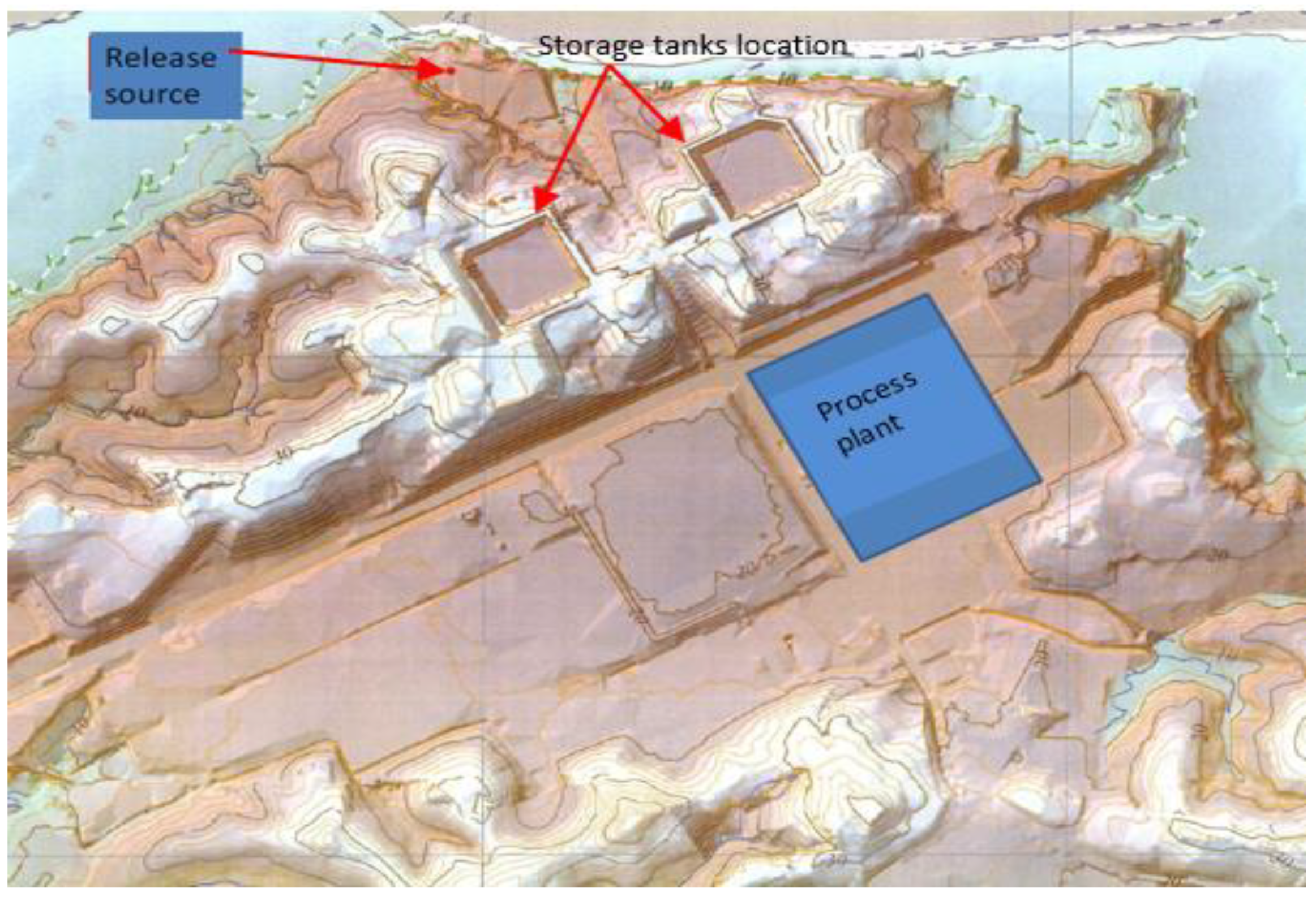
Figure 1.
Schematic diagram showing the layout of key items. North is approximately top of the figure.
Figure 1.
Schematic diagram showing the layout of key items. North is approximately top of the figure.

Figure 2.
An example of grid layout across and close to the vent stack. The colour of contours of concentration is not important here and is shown for illustration.
Figure 2.
An example of grid layout across and close to the vent stack. The colour of contours of concentration is not important here and is shown for illustration.

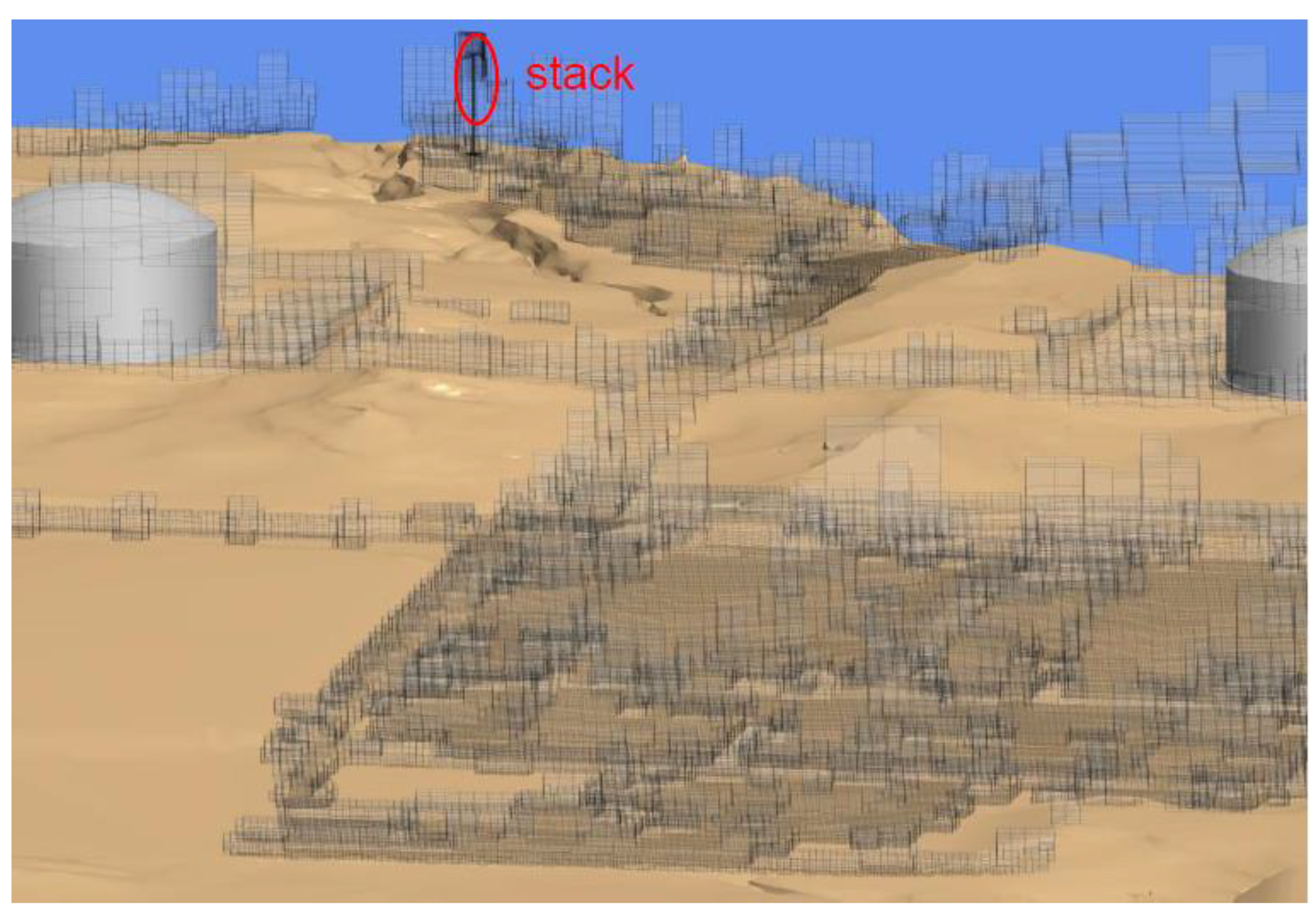
Figure 3.
CFD geometric model showing smaller elements modelled on a subgrid scale basis with source terms applied locally.
Figure 3.
CFD geometric model showing smaller elements modelled on a subgrid scale basis with source terms applied locally.

Figure 4.
Plume iso-surfaces to represent ice and liquid water for a mass fraction (mf) of 0.001.

Figure 5.
Schematic diagram showing the four wind directions. A target area on the first LNG train is also shown; the gas concentration calculated for this area will be used for comparison.
Figure 5.
Schematic diagram showing the four wind directions. A target area on the first LNG train is also shown; the gas concentration calculated for this area will be used for comparison.

Figure 6.
A 3D depiction of the calculated plume envelops for 4 gas concentrations (100% LFL, 50% LFL, 20% LFL and 10% LFL).
Figure 6.
A 3D depiction of the calculated plume envelops for 4 gas concentrations (100% LFL, 50% LFL, 20% LFL and 10% LFL).

Figure 7.
Case 1: iso-surface of 25 kg/s plume, 2 m/s wind, direction 1.

Figure 8.
Case 1: concentric 10 m bands showing concentrations at gas detector location. The blue circle at the centre corresponds to the first 10 m band, the grey circle 10 to 20 m band, etc. The concentrations are the mean values in each band.
Figure 8.
Case 1: concentric 10 m bands showing concentrations at gas detector location. The blue circle at the centre corresponds to the first 10 m band, the grey circle 10 to 20 m band, etc. The concentrations are the mean values in each band.

Figure 9.
Case 1a: iso-surface of 30 kg/s plume, splitting and touching down at two locations leading to different ground concentrations.
Figure 9.
Case 1a: iso-surface of 30 kg/s plume, splitting and touching down at two locations leading to different ground concentrations.

Figure 10.
Case 1b: iso-surface of 45 kg/s plume, 2 m/s wind, direction 1.

Figure 11.
Corresponding ground level LFL concentration for a 25, 30 and 45 kg/s releases at a wind speed of 2 m/s and wind direction 1, showing the touchdown locations and ground level plumes.
Figure 11.
Corresponding ground level LFL concentration for a 25, 30 and 45 kg/s releases at a wind speed of 2 m/s and wind direction 1, showing the touchdown locations and ground level plumes.

Figure 12.
Case 2: iso-surface of 25 kg/s plume, 2 m/s wind, direction 2.

Figure 13.
Case 2a: iso = surface of 30 kg/s plume, 2 m/s wind, direction 2.

Figure 14.
Corresponding ground level LFL concentration for a 25 and 30 kg/s releases at 2 m/s, direction 2 and 3, showing the touchdown locations and ground level plumes.
Figure 14.
Corresponding ground level LFL concentration for a 25 and 30 kg/s releases at 2 m/s, direction 2 and 3, showing the touchdown locations and ground level plumes.

Figure 15.
Ground level LFL concentration for 16 kg/s vent rate at different wind directions and speeds.
Figure 15.
Ground level LFL concentration for 16 kg/s vent rate at different wind directions and speeds.

Figure 16.
Calculated plume compared with a picture of visible plume providing qualitative comparison.
Figure 16.
Calculated plume compared with a picture of visible plume providing qualitative comparison.


Table 1.
Summary table of results showing the ground level concentration at the target area shown in Figure 5.
Table 1.
Summary table of results showing the ground level concentration at the target area shown in Figure 5.
| Case No. | Vent Rates (kg/s) | Wind Directions | Wind Speed (m/s) | Concentration (% LFL) |
|---|---|---|---|---|
| 1 | 25 | 1 | 2 | 3.7 |
| 1a | 30 | 1 | 2 | 4 |
| 1b | 45 | 1 | 2 | 12.5 |
| 2 | 25 | 2 | 2 | 5.5 |
| 2a | 30 | 2 | 2 | 6.3 |
| 3 | 25 | 3 | 2 | 3.8 |
| 3a | 30 | 3 | 2 | 3 |
| 4 | 16 | 4 | 3.9 | 0 |
| 5 | 16 | 5 | 3 | 3.7 |
| 6 | 16 | 5 | 3.9 | 0 |
Publisher’s Note: MDPI stays neutral with regard to jurisdictional claims in published maps and institutional affiliations. |
© 2021 by the authors. Licensee MDPI, Basel, Switzerland. This article is an open access article distributed under the terms and conditions of the Creative Commons Attribution (CC BY) license (https://creativecommons.org/licenses/by/4.0/).
Share and Cite
MDPI and ACS Style
Tan, F.; Tam, V.H.Y.; Savvides, C. Elevated LNG Vapour Dispersion—Effects of Topography, Obstruction and Phase Change. Eng 2021, 2, 249-266. https://0-doi-org.brum.beds.ac.uk/10.3390/eng2020016
AMA Style
Tan F, Tam VHY, Savvides C. Elevated LNG Vapour Dispersion—Effects of Topography, Obstruction and Phase Change. Eng. 2021; 2(2):249-266. https://0-doi-org.brum.beds.ac.uk/10.3390/eng2020016
Chicago/Turabian StyleTan, Felicia, Vincent H. Y. Tam, and Chris Savvides. 2021. "Elevated LNG Vapour Dispersion—Effects of Topography, Obstruction and Phase Change" Eng 2, no. 2: 249-266. https://0-doi-org.brum.beds.ac.uk/10.3390/eng2020016