The Roles of Protein Structure, Taxon Sampling, and Model Complexity in Phylogenomics: A Case Study Focused on Early Animal Divergences

Abstract

Despite the long history of using protein sequences to infer the tree of life, the potential for different parts of protein structures to retain historical signal remains unclear. We propose that it might be possible to improve analyses of phylogenomic datasets by incorporating information about protein structure. We test this idea using the position of the root of Metazoa (animals) as a model system. We examined the distribution of “strongly decisive” sites (alignment positions that support a specific tree topology) in a dataset comprising >1500 proteins and almost 100 taxa. The proportion of each class of strongly decisive sites in different structural environments was very sensitive to the model used to analyze the data when a limited number of taxa were used but they were stable when taxa were added. As long as enough taxa were analyzed, sites in all structural environments supported the same topology regardless of whether standard tree searches or decisive sites were used to select the optimal tree. However, the use of decisive sites revealed a difference between the support for minority topologies for sites in different structural environments: buried sites and sites in sheet and coil environments exhibited equal support for the minority topologies, whereas solvent-exposed and helix sites had unequal numbers of sites, supporting the minority topologies. This suggests that the relatively slowly evolving buried, sheet, and coil sites are giving an accurate picture of the true species tree and the amount of conflict among gene trees. Taken as a whole, this study indicates that phylogenetic analyses using sites in different structural environments can yield different topologies for the deepest branches in the animal tree of life and that analyzing larger numbers of taxa eliminates this conflict. More broadly, our results highlight the desirability of incorporating information about protein structure into phylogenomic analyses.

1. Introduction

The relationship between protein structure and the patterns of sequence evolution has been a topic of interest since the very dawn of molecular evolution as a field [1,2] and, despite the very limited amount of data available at the time of those early studies, many of those early hypotheses have stood the test of time (reviewed by Alvarez-Ponce [3]). Our understanding of the factors that determines rates of amino acid change have certainly expanded since those pioneering studies [4,5], but two important constants have been the idea that the buried residues in globular proteins evolve more slowly [6,7,8] and are more hydrophobic than solvent-exposed residues [8,9]. Likewise, relative amino acid exchangeabilities also differ among structural environments [7,10,11]. However, the relationship between protein structure and the retention of historical signals that can provide information about the relationships among organisms is far less clear.

Our ability to understand relationships among organisms was revolutionized by the rapid accumulation of transcriptome and whole genome sequence data. In fact, the impact of increased data availability has been so profound that many biologists have expanded the term phylogenomics—a term originally applied to the use of evolutionary analysis to improve predictions of protein function [12,13]—to the broader effort to understand the tree of life [14]. Although the phylogenomic approach has had many successes, a number of specific relationships have remained unresolved despite intensive study. The position of the metazoan root—the earliest divergence among animals—has proven to be one of the most challenging relationships to resolve. Despite extensive study [15,16,17,18,19,20,21,22,23,24,25,26,27,28,29,30], three trees remain plausible (Figure 1). Protein structure may play an important role in efforts to understand the position of the metazoan root. Pandey and Braun [31] analyzed a large (231 proteins) data matrix and they found that phylogenetic analyses of solvent-exposed sites using standard methods support T2, whereas similar analyses of buried sites in the same proteins support T3 (T2 and T3 are defined in Figure 1).

Recovery of different positions of the root when buried vs. exposed sites are analyzed suggests that deep metazoan phylogeny might be useful as a model system to explore the relationship between phylogenetic signal and protein structure. Cases where standard phylogenetic analyses using different subsets of the genome yield different tree topologies with relatively high support have been attributed to “data-type effects” [35,36]. Data-type effects are defined as follows: if phylogenetic analyses using subsets of the genome defined using non-phylogenetic criteria yield different topological signals, one can be said to have identified a data-type effect. The subsets of the genome must be large enough to overcome sampling error and the data types must be defined before conducting the phylogenetic analysis. In the specific case studied by Pandey and Braun [31], the relevant subsets of the genome are sites encoding amino acids in different structural environments. In principle, data-type effects can be explained in two ways: (1) the topology recovered for at least one of the data types is incorrect, or (2) the data types are associated with different underlying trees. The first explanation is relatively straightforward: if one of the data types has a poor fit to the model(s) used for phylogenetic analyses, then model misspecification might result in an incorrect estimate of phylogeny. The second explanation is more complex, and it represents one of the biggest challenges in the field of phylogenomics: different parts of the genome can have distinct evolutionary histories [37,38]. If we restrict our attention to proteins encoded by orthologous loci (the typical approach in phylogenomics [39]), incomplete lineage sorting (ILS) is likely to be the most common source of genuine discordance among gene trees (see chapter 10 of Warnow [40] for review). In fact, it is possible to make a clear prediction if ILS represents a major source of conflict: given a set of three plausible trees (e.g., Figure 1), we should find evidence supporting a majority topology that corresponds to the species tree and equal support for the two minority topologies [41]. However, despite the importance of considering discordance among gene trees in phylogenomic studies, ILS (or any other sources of genuine discordance among gene trees) is not a viable explanation for the topological differences observed by Pandey and Braun [31]. The nucleotides that encode exposed and buried sites in any specific protein will be interspersed in the same transcription unit, sometimes immediately adjacent to each other. Although distinct gene trees can underlie different proteins, there is no plausible mechanism that would lead to the existence of one tree (or set of trees) for exposed sites and a distinct tree (or trees) for buried sites if the exposed and buried sites are sampled from gene(s) encoding the same protein(s). Thus, we can exclude the second explanation for data-type effects and focus on the issue of model fit.

The data-type effect observed by Pandey and Braun [31] was initially observed in analyses using “standard models” (e.g., the Le-Gascuel (LG) model [42] or the 20-state version of the Tavaré [43] general time reversible (GTR) model). However, analyses conducted after recoding amino acid data eliminated the conflict [31]. Analyses of exposed and buried sites conducted after lumping physicochemically similar amino acids (into the six Dayhoff et al. [44] categories) both yielded T2; likewise, analyzing both data types as two-state (purine/pyrimidine) nucleotide data also yielded T2. Amino acid recoding is intended to reduce misleading signal due to saturation and/or changes in amino acid frequencies [45]. Thus, the observation that analyses of both data types yield T2 after these analyses suggests that the signal associated with buried sites is misleading. This seems surprising given the lower rate of evolution for buried sites [6,7,8]. Moreover, amino acid recoding is an unsatisfying analytical approach, and it seems more logical to analyze unmodified amino acid data using more “biologically realistic” models of evolution.

Models that incorporate site-specific state frequencies are the most common of these more biologically realistic models of sequence evolution. The development of those can be traced to the framework proposed by Bruno [46] and Halpern and Bruno [47]. The Halpern–Bruno framework showed that there is a direct relationship between the frequencies of amino acids at individual sites and the strength of selection on each amino acid (at least under the special situation where mutation rates are sufficiently low for each new mutation to be fixed or lost before the next mutation). Although that condition may not be met in real populations, the results of laboratory deep mutagenesis studies [48,49,50,51] are consistent with the idea that amino acid fitness profiles are site specific. The evidence that the basic Halpern–Bruno framework successfully reconciles protein structure and biophysics with population genetics has led to the development of models suitable for phylogenetic analyses. Examples of “Halpern-Bruno-type” models (defined broadly) include the CAT [52] model, which can be used in the Bayesian framework, and the CAT-like model of Le et al. [53] (which Pandey and Braun [31] called “LGL mixtures,” using the first letter of the name of each author), which can be used in either a Bayesian or a maximum likelihood (ML) framework. The CAT model appears to reduce phylogenetic artefacts such as long-branch attraction [54] and it seems reasonable to postulate that similar models (like the LGL mixtures) will exhibit similar behaviors.

The biological realism of those models is desirable, but memory and compute time requirements can become prohibitive for the CAT model (and related models) as the number of mixture classes (sets of equilibrium amino acid frequencies) increases. This can make the CAT model intractable for analysis of phylogenomic datasets, even when parallel or multicore implementations are used [55,56]. In general, memory and compute time requirements increase as a multiple of k (the number of mixture classes) for CAT. Wang et al. [56] proposed the posterior mean site frequency (PMSF) method, improving this to a multiple of ~k/1.5 and using substantially less random-access memory(RAM). PMSF assigns a conditional mean amino acid frequency profile to each site using a preliminary guide tree, and those profiles can then be used for in-depth tree searching and per site likelihood calculation in place of the full mixture model. Despite this improvement, PMSF is still computationally burdensome and therefore remains difficult to use in analyses of taxon-rich phylogenomic datasets. Nevertheless, the PMSF approach would appear to provide a way to add biological realism and ameliorate data-type effects due to protein structure.

An alternative to the use of complex and realistic models of sequence evolution, with their associated computational burden, has been recognized for more than a decade: adding taxa to phylogenetic analyses [57,58]. Including large numbers of taxa in phylogenetic analyses almost always improves the accuracy of those analyses [59,60,61,62], with only a small number of exceptions [63]. The positive effects of adding taxa to phylogenies have often been attributed to the breaking up of long branches; thus, one major impact of adding taxa is expected to be a reduced likelihood of long-branch attraction [64,65]. Adding taxa can also improve phylogenetic analyses by improving parameter estimates in model-based analyses [66,67]. However, it is important to recognize that the original taxon-sampling results [57,58] were obtained for analyses using the parsimony criterion, which has been criticized as unrealistic [68,69]. However, when viewed another way, the ability of increased taxon sampling to improve phylogenetic estimation using the “unrealistic” parsimony criterion could be viewed as a positive: it suggests that analyses of a taxon-rich dataset might yield accurate estimates of phylogeny even if less “realistic” models (like the site-homogeneous LG model [42]) are used for analyses. It is now possible to collect large amounts of data from many different taxa, making it possible to generate taxon-rich phylogenomic trees.

For this study, we have used early metazoan phylogeny as a model system to examine which factor (taxon sampling or model realism) is more important to ameliorate the structural data-type effect noted by Pandey and Braun [31]. Since phylogenetic estimation using complex models and datasets is a difficult computational problem, even when the relatively efficient PMSF method is used, we focused on a metric of phylogenetic signal that can be calculated in a rapid manner. Specifically, we used the numbers of strongly decisive sites supporting each of the three plausible topologies for the base of Metazoa (Figure 1). We define strongly decisive sites in a manner that generalizes the approaches used by Kimball et al. [70] and Francis and Canfield [29]. This definition allows us to identify sites that strongly favor each specific tree relative to all other plausible trees in a set of candidate trees. We expected the strongly decisive sites criterion to make it possible to examine protein structure data-type effects for a taxon-rich data matrix using both simple site-homogeneous and complex site-heterogeneous models. For these analyses, we used the Simion et al. [26] dataset, which comprises more than 1500 orthologous proteins sampled from 97 taxa and includes all major metazoan clades. We examined the number of strongly decisive sites in the two relative solvent accessibility (RSA) classes (surface residues and buried residues) and in three secondary structure (SS) classes (helix, sheet, and coil) given different models and numbers of taxa. These results allowed us to extend the examination of phylogenetic signal and protein structure data types reported by Pandey and Braun [31].

2. Methods

We used the globular proteins in the Simion et al. [26] dataset, subdividing those proteins using structural criteria, and conducting ML analyses of each structural component individually. We began by identifying and eliminating transmembrane proteins. We did this by using the TopCons prediction server [71] to identify a total of 153 transmembrane proteins which we excluded to create the “filtered Simion et al. dataset” (hereafter, the “FSD”). The FSD comprised 1566 globular proteins with 356,014 aligned sites and 39% missing data. The globular proteins were then subdivided using either RSA or SS, as described by Pandey and Braun [11,31]. Briefly, we assigned structural information to sites in each alignment using a weighted consensus sequence, and the consensus amino acid at each position was the residue with the highest Henikoff and Henikoff [72] weight. The consensus sequences were used as input for SCRATCH-1D [73], a suite of neural network programs for protein structure prediction (ACCpro for RSA and SSpro for SS). This pipeline, available from github (see data availability statement), creates a nexus file [74] for each multiple sequence alignment with a sets block that has charsets for the two RSA classes (Exposed and Buried) and the three SS-based classes (Helix, Sheet, and Coil). These sets blocks allowed us to use PAUP* 4.0b10 [75] to extract each subset of the data. The annotated nexus files are available in Supplementary File S1.

The FSD included 97 taxa: 25 Choanozoa outgroups, 12 Ctenophora, 25 Porifera, and 33 additional metazoans (23 Cnidaria, 9 Bilateria, and the placozoan Trichoplax adhaerens). To examine the effects of taxon sampling on tree searches and proportions of strongly decisive sites, we randomly sampled 40 combinations of taxa that included one sponge, one ctenophore, one cnidarian, six outgroups, and all sampled bilateria (yielding data matrices with a total of 19 taxa). We then added taxa to these sparse taxon samples in a manner that is often used by systematists: by adding relatively distant relatives of the taxa that are already included in the data matrix. This strategy will subdivide long branches as much as possible. Specifically, we took each 19-taxon dataset and added four sponges (one from each class), two ctenophores, and two cnidarians (one from each subphylum), yielding 27-taxon datasets. This procedure was repeated three additional times, generating 35, 43, and 51 taxon extensions of each of the 40 19-taxon datasets.

The number of decisive sites (as defined by Kimball et al. [70]) favoring each topology is likely to provide a useful criterion to examine different topologies. Because this manuscript has an interdisciplinary target audience, we will provide a brief description of the likelihood calculations. Interested readers are referred to reviews on the topic (e.g., chapter 8 of Warnow [40]) for additional details. Briefly, the likelihood is proportional to the probability of the data (the site patterns in the alignment) given the tree with branch lengths. If we consider the simplest possible alignment (two sequences), we can use Equation (1) to calculate the probability that a site will be occupied by amino acid j after time t given that the initial state is amino acid i:

P(t) = exp(Qt),

(1)

where P(t) is a matrix of probabilities that the site is occupied by amino acid j after time t given that the initial state is amino acid i, and Q is the instantaneous rate matrix. Time (t) is the branch length in units of substitutions per site (other units would require information about the substitution rate). Most models of sequence evolution used in empirical studies are time reversible, and time reversibility makes it possible to write Q as the product of a symmetric matrix of amino acid exchangeabilities and diagonal matrix (Π) with the equilibrium frequencies of each amino acid [76,77]. The Felsenstein [78] pruning algorithm can be used to calculate the likelihood that the complete alignment is simply the product of the likelihoods of all sites (in practice, the sum of the log likelihoods is used). Since trees for multiple taxa will have unknown internal states (i.e., the ancestral states at each node), all possible states are used for each node and the marginal likelihood is calculated. The branch lengths (and any other free parameters in the model) are obtained by numerical optimization. Amino acid frequencies are part of the Q matrix (via the Π matrix), so likelihoods are obtained using the Halpern–Bruno framework by using a mixture model framework or by assigning different matrices to each site. In practice, these calculations are performed by efficient ML programs, such as RAxML [79] and IQ-TREE [80].

This review of likelihood calculations makes two points: (1) each site has an associated site likelihood, and (2) there is no consideration of flanking sites in the site likelihood calculations. The first property allows us to define a decisive site as a site favoring a specific topology (Ta) relative to one or more other candidate topologies (Tb, Tc, ...) given the likelihood criterion. The degree to which site i supports a specific topology can be calculated using per site likelihoods (obtained from RAxML or IQ-TREE) using Equation (2):

$$\mathsf{\Delta }\ln L_i^{T\mathrm{a}}=\max \left(\ln L_i^{T\mathrm{b}}, \ln L_i^{T\mathrm{c}},\dots \right) - \ln L_i^{T\mathrm{a}},$$

(2)

where $\ln L_i^T$ is the likelihood for site i given topology T. $\mathsf{\Delta }\ln L_i^{T\mathrm{a}}$ will be positive for sites that favor Ta and negative if one (or more) of the other candidate topologies is favored relative to Ta. We examined three candidate topologies for this study, but Equation (1) can be used for any number of candidate topologies. We designated sites with ΔlnL ≥ 5 standard deviations from the mean ΔlnL value as strongly decisive sites (see Supplementary Figure S1 for additional details). Separating the FSD into subsets defined by RSA and SS addresses the absence of spatial information in the likelihood calculations (the second point we highlighted) by restricting analyses to specific structurally defined site types.

We used RAxML 8.2.10 for tree searches and site likelihood calculations using simple, site-homogeneous models. Specifically, we used the 20-state GTR model with Γ-distributed rates across sites (i.e., GTR₂₀ + Γ). The large number of sites in each dataset (larger than 160,000 sites for each RSA structural class) led us to estimate GTR₂₀ model parameters from subsets of the data. Briefly, we generated 10 random datasets with all 97 taxa and 10,000 sites from each structural class. Then, we conducted a tree search and optimized parameters in RAxML, using a random starting tree for each 10,000-site dataset. The GTR₂₀ model parameters (equilibrium amino acid frequencies and the exchangeability matrix) estimated for each site subsample were then averaged, and these averages were used as the GTR₂₀ model parameters for each structural class. These rate matrices are available in Supplementary File S1.

We used IQ-TREE 1.5.1 to estimate per site likelihoods for site-heterogeneous models. Specifically, we used the PMSF approach with five 25,000-site datasets (sites randomly sampled from the complete data matrix). PMSF requires a starting tree with branch length estimates to generate the site-specific frequency profiles, and we used the RAxML GTR₂₀ + Γ tree for this. All PMSF analyses used the LG exchangeability matrix. We used six different numbers of site categories (i.e., we used LG + C10 + PMSF + Γ, LG + C20 + PMSF + Γ, and so forth, up to C60). We chose this sample size based on preliminary tests with the exposed site data. Those tests revealed that compute time and memory requirements (>150 GB per core) became prohibitive for 50,000-site datasets when we used the largest number of profile mixture categories (C50 and C60). We repeated the site likelihood calculations using the site-homogeneous GTR₂₀ + Γ model in IQ-TREE to determine whether the specific implementation of those models in each program had any impact on our inferences (as might occur, for example, if there are differences between RAxML and IQ-TREE in the details of the numerical optimization).

We examined model fit using the sample-size corrected Akaike information criterion (AIC_c) [81]. In most cases, we simply used the AIC_c value from the ‘.iqtree’ output file. However, determining whether RSA or SS subdivision resulted in a better overall fit to the data required us to sum the likelihoods for each data subset and then calculate the AIC_c. The branch length estimates for each structural partition were unlinked, so we included all branch lengths as free parameters in the AIC_c calculation (i.e., we used two times the number of branches for RSA and three times the number of branches for SS).

3. Results

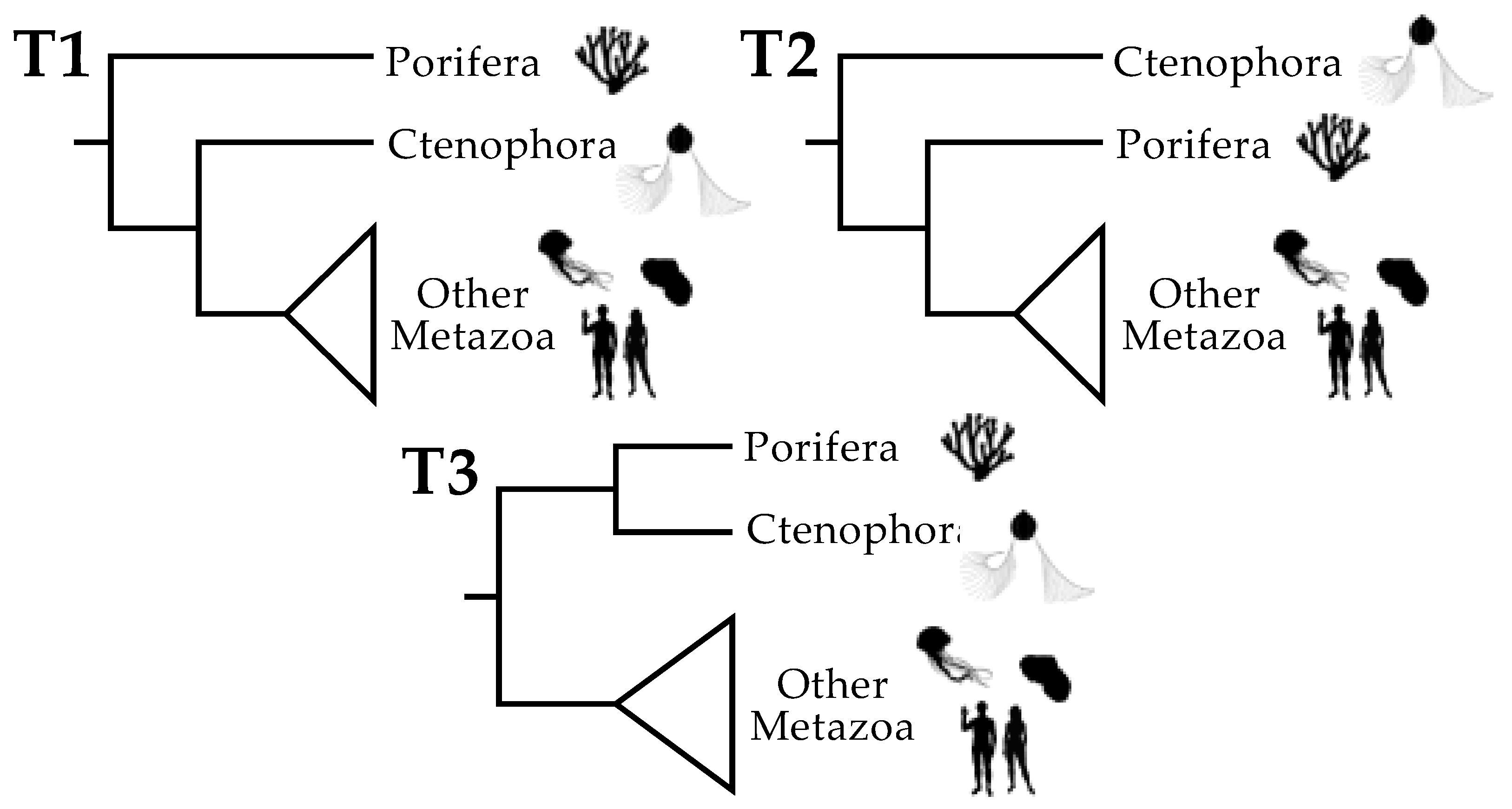
3.1. Tree Searches and the Use of Strongly Decisive Sites Lead to Similar Conclusions

Because we used the strongly decisive site criterion (i.e., the view that the tree with the largest number of strongly decisive sites is the best-corroborated tree), we believed it was important to establish that it yields conclusions similar to those for standard tree searches. The proportion of strongly decisive sites supporting T2 was much larger than the proportions supporting either T1 or T3 when the complete FSD was examined (

Table 1. Percentages of strongly decisive (SD) sites in the complete FSD.

Dataset	T1	T2	T3	SD Sites 1	Total Sites
Exposed	19.3	70.8	9.9	1420	161,897
Buried	16.6	66.1	17.3	1625	194,117
Helix	19.2	69.3	11.5	1290	161,117
Sheet	12.5	71.6	16.9	514	60,563
Coil	17.7	68	14.3	1194	134,334

¹ Calculated using the 20-state general time reversible model with gamma-distributed rates across sites (GTR₂₀ + Γ) model with parameters optimized on each subset of the data.

). Tree searches using RAxML resulted in topology T2 with 100% bootstrap support in all cases, indicating that using the proportion of decisive sites yields conclusions that are similar to those of tree searches. However, some strongly decisive sites supporting T1 and T3 were present despite the strong support for T2 in the bootstrap analyses.

In sharp contrast to analyses using all taxa, tree searches using the most reduced taxon set (40 replicates of 19 taxa subsampled from the FSD dataset, see Methods Section for details) resulted in all three topologies. In all cases, analyses using either tree searches or the strongly decisive sites criterion indicated that T2 was the most common topology (Figure 2). However, the number of times each topology was recovered differed between the exposed and buried sites: T3 was more common in the analyses of buried sites, as we expected based on Pandey and Braun [31]. These results corroborate the exposed vs. buried site data-type effects hypothesis for the root of Metazoa, although they also indicate that the effect is weak. Moreover, we found that the results based on strongly decisive sites were similar to those for tree searches, although they did not yield identical results (Figure 2). Specifically, the strongly decisive sites criterion revealed greater support for T3 than did tree searches when datasets with the small taxon samples were analyzed.

The somewhat distinct behavior of using tree searches to identify the ML topology and examining the strongly decisive sites emphasizes a potential benefit of the latter method: it provides information about the relative support for multiple contradictory topologies. For the 19-taxon datasets, there were more sites that supported T3 than T1, but this was obscured because most tree searches returned T2 as the optimal tree. Likewise, there were a few tree searches for both site classes that yielded T1 but there was no taxon sample for which T1 was optimal given the strongly decisive sites criterion (Figure 2). These results emphasize that, in contrast to tree searches, consideration of the strongly decisive sites can provide information about the relative support for topologies that are suboptimal given the ML criterion.

In contrast to the results of analysis using the sparse taxon sets, for analyses using all 97 taxa, the FSD consistently resulted in a large number of strongly decisive sites supporting T2 and nearly equal (but much lower) numbers of sites supporting T1 and T3. One possible interpretation of strongly decisive sites is that they reflect bipartitions in gene trees (for details see Discussion, Section 4.1). If true, the simplest expectation is that the number of strongly decisive sites supporting the two minority topologies would be equal. We tested the null hypothesis of equality for the numbers of strongly decisive sites supporting T1 and T3 (Supplementary File S2), and we were unable to reject the null hypothesis for buried or sheet residues (χ² for buried = 0.262, χ² for sheet = 2.22; both p > 0.1). In contrast, the null hypothesis could be rejected for exposed and helix residues (χ² for exposed = 42.6, χ² for helix = 25.3; both p < 10⁻⁶); however, the number of strongly decisive sites favored T1 relative to T3 for both the exposed and helix sites. The remaining case (coil residues) was not significant after a multiple test correction (χ² for coil = 4.19; p = 0.0407), but it also favored T1 relative to T3. Thus, taxon addition appears to cause support, as measured using strongly decisive sites, to shift away from T3 toward T2 (the best-supported tree overall) and T1.

The overall likelihood when the data were subdivided using RSA was much better than that for subdivision based on SS (ΔlnL favoring subdivision by RSA = 84,985.12), and since RSA subdivision actually introduces fewer free parameters the SS subdivision, it will also be favored by the AIC_c criterion (Supplementary File S2). The better fit of the RSA model could reflect the relatively large difference in mean substitution rates for the two RSA categories (the substitution rate for exposed sites is 1.67× the buried site rate; Supplementary File S2). In contrast, the difference between the SS category with the highest mean rate (helix residues) and the slowest SS rate category (sheet residues) is only 1.21× (Supplementary File S2). We note, however, that the equilibrium amino acid frequencies for all subsets of the data also exhibited substantial differences (Supplementary File S2) and this is likely to contribute to the fit of the alternative models. The amino acid frequencies conformed to our expectations; for example, polar amino acids dominated the solvent-exposed positions, whereas hydrophobic amino acids were more common in the buried environment. Likewise, the equilibrium amino acid frequencies for sites in helix and sheet environments were enriched for residues favored in each of those environments, and the equilibrium frequencies of proline and glycine were also elevated relative to other environments for the coil residues. Finally, the rate matrix exchangeabilities for the exposed and buried sites were similar to those observed by Pandey and Braun [11,31] (the estimated rate matrices and a spreadsheet with rate matrix comparisons are available in Supplementary File S1).

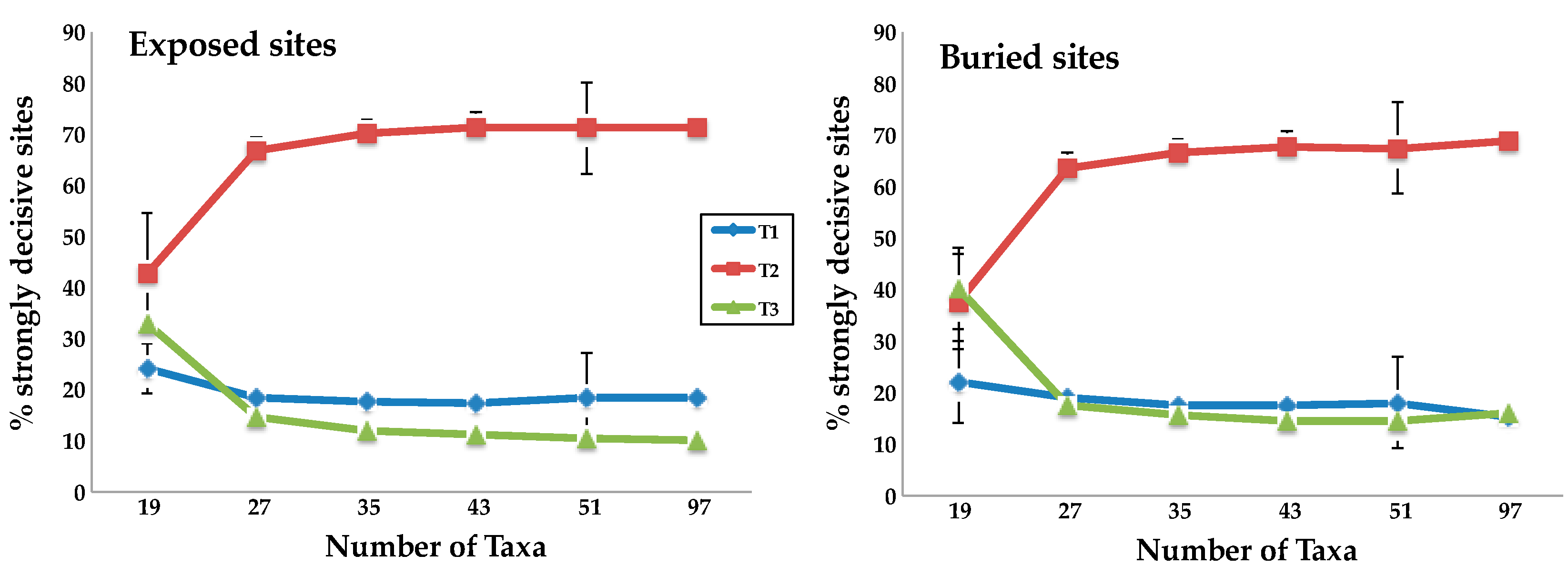
3.2. Taxon Addition Leads to Rapid Convergence in the Proportions of Strongly Decisive Sites Observed Using the Complete Taxon Sample

When we gradually increased the number of taxa from 19, creating datasets that included 27, 35, 43, and 51 taxa, the proportion of decisive sites supporting T2 increased for all structural subsets. The most dramatic increase in the number of decisive sites supported T2 topology between 19-taxon and 27-taxon sets for all the structurally defined subsets of the data (Figure 3 and Supplementary Figure S2). Indeed, when we used the strongly decisive sites criterion to analyze the buried sites and sheet residues, we actually observed a shift in support from T3 (for the 19-taxon datasets) to T2 (for all other taxon sets). The exposed, helix, and coil subsets always supported T2, but the proportion of strongly decisive sites supporting T2 was only slightly greater than the proportion supporting T3. The proportion of sites supporting T2 increased sharply as soon as taxa were added. For all structural classes, the increase in the number of strongly decisive sites favoring T2 largely saturated once we included 35 taxa and remained virtually constant until we reached the complete set of 97 taxa.

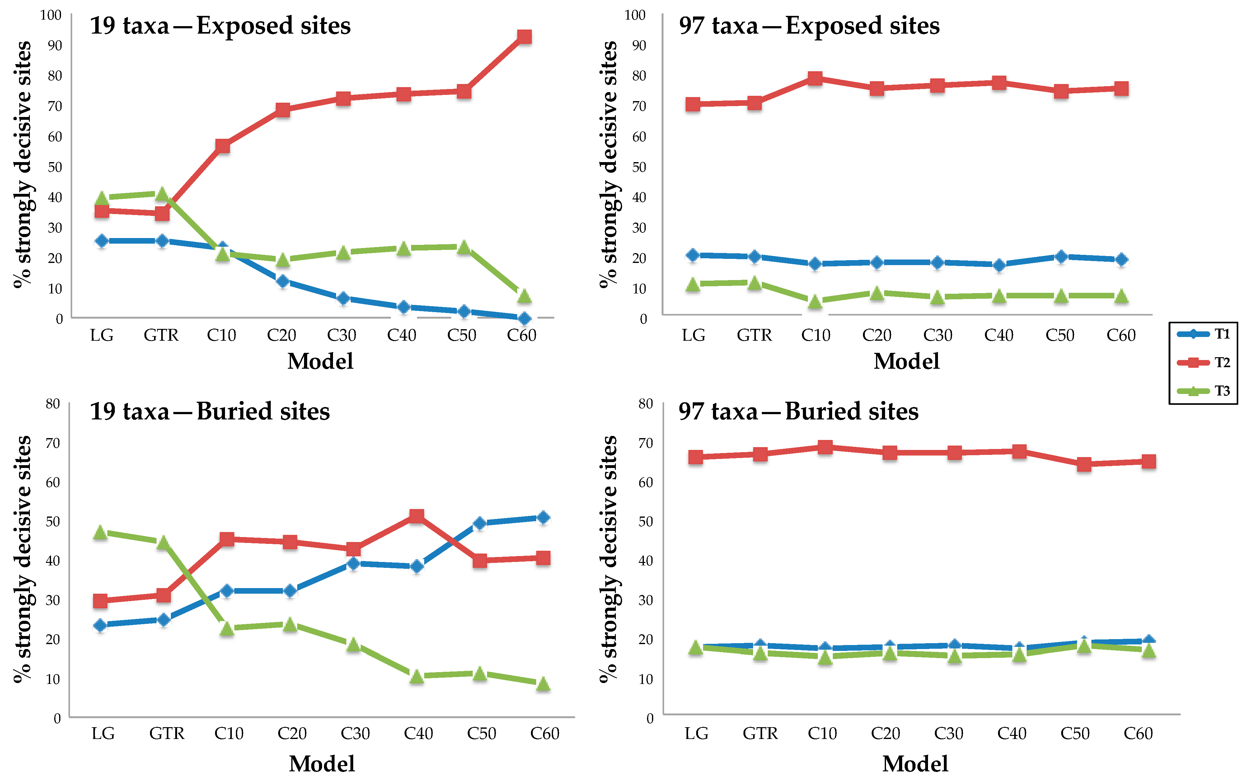
3.3. Rich Taxon Sampling Can Compensate for Low Model Complexity

It is generally assumed that less-complex (and, presumably, less biologically realistic) models will be more prone to bias than parameter-rich models. This led us to examine the impact of increased taxon sampling on the relatively simple site-homogeneous models (GTR₂₀) and the site-heterogeneous models (LG + PMSF), comparing 19-taxon datasets to those with 97 taxa (in all cases, we used random samples of 25,000 sites). As above, we reduced dataset heterogeneity before conducting any analyses by dividing our data into structurally defined subsets. Adding among-sites heterogeneity in amino acid frequencies using the PMSF approach improved model fit relative to site-homogeneous models for all data subsets. In fact, the model with the largest number of mixture classes (i.e., LG + C60 + PMSF + Γ) was always the best fitting model for both the 19- and 97-taxon datasets based on AIC_c scores (Supplementary File S3). However, the relationship between model complexity and proportions of strongly decisive sites supporting each topology differed substantially for the 19- and 97-taxon datasets. For the 19-taxon dataset, the proportions of strongly decisive sites supporting each topology were highly unstable as the complexity of the model increased from LG to C60 (Figure 4 and Supplementary Figure S3). Moreover, the topology with the largest number of strongly decisive sites in the 19-taxon dataset was T3 when the site-homogeneous models (i.e., the LG and GTR₂₀ models) were used but the support generally shifted to T2 when site-heterogeneous models were used. However, the situation was even more complex, since the support actually underwent another shift (to T1) when the 19-taxon buried site dataset was analyzed using the C50 and C60 mixtures. In sharp contrast to the case for the 19-taxon datasets, all analyses using the 97-taxon dataset supported T2. Moreover, the proportions of strongly decisive sites supporting each topology was remarkably stable across models in analyses of the 97-taxon dataset (Figure 4 and Supplementary Figure S3).

4. Discussion

These analyses showed that the protein structure data-type effect found by Pandey and Braun [31] could be replicated using another dataset, although the data-type effect appeared to be relatively weak. This was not especially surprising since Pandey and Braun [31] noted that conducting analyses after reducing the set of outgroups to choanoflagellates yielded T2 regardless of whether exposed or buried sites were analyzed. The FSD only included choanoflagellate outgroups, so it might be reasonable to expect the signal supporting T3 to be especially weak; however, there was a clear difference between exposed and buried sites for small taxon samples (Figure 2). However, there were also conflicting signals in the data and adding taxa rapidly eliminated the weak tendency for analyses of buried sites to support T3 (Figure 3). Our taxon sampling results also provide evidence against T3; after all, it has long been appreciated that adding taxa improves the performance of phylogenetic analyses (reviewed by Heath et al. [65]). The proportion of strongly decisive sites supporting T3 decreased as taxa were added and the proportion of sites supporting T2 (ctenophores sister to other Metazoa) increased (Figure 2). The proportion of strongly decisive sites supporting T1 was always smaller than the proportion supporting T2 and it was relatively stable to taxon addition. It was only necessary to add a small number of taxa for the proportions of strongly decisive sites that support each topology to converge on the values for the complete 97-taxon dataset. We also found that the proportions of decisive sites identified using simple homogeneous models is virtually identical to that proportions found using complex models when taxon-rich datasets were analyzed. The latter finding is highly significant, since the relatively simple site-homogeneous models of sequence evolution impose a limited computational burden relative to analyses using more complex models.

Given the programs currently available for phylogenetic analyses, the strongly decisive sites criterion cannot replace standard tree searches using the ML criterion or commonly used support metrics, like the bootstrap. However, it is useful for several reasons. First, as we have already emphasized, it is a computationally efficient approach that can provide information about support for multiple alternative trees. Examining support for alternative trees is especially straightforward when the plausible tree space is small, as it was for this study (Figure 1), but it would also be possible to perform a tree search and then focus on poorly supported nodes (e.g., by identifying strongly decisive sites for the optimal tree and the two trees produced by nearest-neighbor interchanges for each poorly supported node). Second, focusing on decisive sites highlight unusual genes [70], and genes with anomalously large numbers of strongly decisive sites might reflect very poor model fit or hidden paralogs. No individual genes with an unusually large number of decisive sites were identified in this study (Supplementary File S4). Finally, using strongly decisive sites might limit the impact of model misspecification. Models of sequence evolution are useful tools for inference [68,82] but they never capture “full reality” and there may be cases where no model within a set of candidates is an adequate approximation of the true model [83,84]. Assuming the models used for analyses meet a certain minimum level of “realism”, dividing sites into two categories, only one of which is then viewed as informative, could be useful. Overall, we believe that this approach was useful for analyses focused on the metazoan root, and it seems reasonable to propose that it will be useful for analyses focused on other parts of the tree of life.

4.1. Taxon Sampling Has a Larger Impact Than Model Complexity

To examine the impact of taxon sampling, we adopted a taxon addition strategy consistent with the approach that has long been used by practicing systematists [85]. Specifically, we attempted to maximize the subdivision of long branches instead of adding taxa randomly. We began with a set of randomly chosen 19-taxon datasets and then added taxa likely to be relatively divergent from the taxa that were already present. This taxon addition strategy has a sound theoretical basis [86] and empirical systematists typically add taxa in this manner [65,87,88,89]. The rapid convergence on the proportions of strongly decisive sites that emerges when all 97 taxa are analyzed suggests that extremely dense taxon sampling (e.g., thousands or tens of thousands of taxa) is unlikely to be necessary to make inferences regarding phylogenetic questions similar to the problem we examined. In fact, the recent publication of whole genome assemblies for hundreds of vertebrate taxa [90,91] indicate that the necessary sequencing capacity is available at the time. Addressing questions about the earliest metazoan divergences will present additional challenges, including sample availability and issues of DNA quality [92], but it seems reasonable to assert that the biggest challenges are unlikely to relate to data collection; instead, the most challenging issue is likely to be the analyses.

The positive effects of adding taxa in this study are likely to be a direct outcome of breaking up long branches and reducing the number of unobserved substitutions that need to be inferred as part of the analysis. Breaking up long branches is likely to be especially important for analyses using relatively simple, site-homogeneous models, like GTR₂₀ (as well as the Braun [77] models and empirical models like the LG [42] and Dayhoff/PAM [44] models). Lakner et al. [93] showed that the potential for protein function (more specifically, sequence-to-structure fit assessed using protein threading) decays rapidly when evolution proceeds according to simple models. However, when Lakner et al. [93] examined the paths between empirical sequences (i.e., cases where both ends of the evolutionary path are known to be functional), they found that the sequences along the paths between real sequences were typically consistent with functional tertiary structures. Adding taxa will reduce the lengths of the paths between sequences and should therefore have a positive impact on inference. The fact that the more complex PMSF model did not perform differently from simpler models (based on the proportions of strongly decisive sites) suggests that rich taxon sampling did not have substantial indirect effects (we define indirect effects as cases where the estimate of phylogeny is improved by the more accurate parameter estimates that are possible when many taxa are analyzed). It is possible that adding taxa did provide better information about the expected amino acid frequencies at each site, but even if that is true, the better information about amino acid frequencies does not result in an increased proportion of strongly decisive sites that support a specific topology. One indirect effect that is possible would involve improved estimates of site-specific evolutionary rates [67], and since the simple and the complex models that we used both included among-sites rate heterogeneity parameters, all models are likely to exhibit similar behaviors. Overall, it seems most likely that breaking up long branches was responsible for the observed amelioration of the protein structure data-type effect and that improved estimates of site-specific residue frequencies were not involved.

4.2. Strongly Decisive Sites, Phylogenetic Signal, and Protein Structure

The use of strongly decisive sites as a metric for phylogenetic signal raises an important question: what exactly do they indicate? There are two fundamentally different ways to explain the existence of strongly decisive sites. The first possibility is that strongly decisive sites that emerge in phylogenetic analyses of an aligned gene region might reflect the bipartitions in the phylogenetic tree underlying that gene. This is a straightforward explanation, and it seems reasonable to assert that at least some strongly decisive sites must be accurate indicators of bipartitions in true gene trees (this is likely to be the case as long as the model used for ML analyses can yield an accurate estimate of phylogeny). If it is generally true that the strongly decisive sites define gene tree bipartitions, conflicting decisive sites must reflect genuine discordance among gene trees due to ILS, possibly combined with some other mechanisms that can lead to genuine disagreements among gene trees. The alternative possibility is that strongly decisive sites provide a combination of accurate and misleading information. In this case, conflicting strongly decisive sites might be present even if there is little or no conflict among gene trees. These possibilities are not mutually exclusive; for example, most strongly decisive sites could provide accurate information about the topology of their associated gene trees despite the existence of misleading strongly decisive sites.

Our analyses revealed strongly decisive sites that support all three plausible positions of the metazoan root (Figure 3 and Figure 4); thus, it is critical to consider explanations for strongly decisive sites that can explain conflicting sites. If we embrace the possibility that strongly decisive sites yield accurate information about bipartitions in the true gene trees, we must also explain the fact that approximately 60% of protein alignments with at least two strongly decisive sites have sites that support more than one topology (Supplementary File S4). This can be explained by intragenic recombination, which is especially plausible for deep-branching Metazoa given the large number of introns in the common ancestor of all Metazoa [94]. Large numbers of introns lengthen genes and therefore increase the potential for intragenic recombination. More important questions to ask when considering the question of whether ILS can provide a plausible explanation for discordance among gene trees at the base of Metazoa are: (1) how many generations separating cladogenic events at the base of Metazoa?, and (2) what were the effective population sizes of those ancestral lineages? Neither of these questions have clear answers, but we do note that small-bodied organisms (as the metazoan ancestor is likely to have been) often have extremely large effective population sizes [95]. Large effective population sizes would increase the probability of ILS. Although most studies focused on deep metazoan phylogeny have not considered discordance among gene trees, there have been exceptions. For example, Ewing et al. [96] invoked the possibility that gene tree discordance ILS has led to discordance among gene trees for deep metazoan relationships (albeit for the relationships at the base of Bilateria). Arcila et al. [97] implicitly assumed ILS was possible in their analysis of the metazoan root. We say this because they analyzed gene trees using ASTRAL-II [98], a program that implements a fast method to combine gene trees in manner and obtain an accurate estimate of the species tree when gene trees differ due to ILS (we also note that Arcila et al. [97] concluded that ctenophores are sister to other Metazoa, just as we did in this study). Overall, it seems reasonable to assert that analyses of deep metazoan relationships should consider the possibility of gene tree–species tree discordance, regardless of whether or not strongly decisive sites provide reliable information about gene tree topologies.

It is possible to make specific predictions regarding the expected patterns of disagreement among strongly decisive sites if discordance among gene trees explains the conflict. If the discordance among them reflects ILS alone and the focal question involves a rooted three-taxon species tree (e.g., the plausible trees in Figure 1), the majority gene tree topology will match the species tree and the two minority gene tree topologies will be equiprobable [41]. We were unable to reject the null hypothesis of equality for the two minority topologies when we analyzed buried sites, so ILS could explain the strongly decisive site data for that structural environment (if we subdivide proteins using SS rather than RSA, we would come to a similar conclusion using coil and sheet sites). However, we were able to reject the null hypothesis that there are equal numbers of strongly decisive sites in the two minority categories for exposed residues (and for helix residues when SS was used to subdivide alignments). It is possible to explain asymmetry in the proportions of the two minority gene tree topologies by invoking a model with substantial gene flow among the earliest stem ctenophores, sponges, and Parahoxozoa (e.g., via horizontal gene transfer) if some exchanges were more common than others. The idea that basal metazoan lineages have experienced horizontal gene transfers from divergent lineages is strongly corroborated [99,100,101], hence the notion that there might have been gene transfers among the stem ctenophores, sponges, and Parahoxozoa (and other related lineages, such as choanoflagellates and Filasterea [94,102]). However, both the simple ILS hypothesis and more complex gene transfer hypotheses make one fundamental prediction regarding the proportions of minority gene trees: support for the two minority topologies is expected to be equal for all sites sampled from the genome. This was not what we observed.

The observation that numbers of strongly decisive sites that support each of the two plausible minority topologies is equal for buried sites but unequal for exposed sites ultimately requires at least some of the decisive sites to be misleading (i.e., it is necessary to invoke at least a degree of model inadequacy in analyses of some subsets of the data). In principle, the misleading signal could be associated with buried sites, with exposed sites, or with sites in both structural environments. However, the fact that we were only able to reject equality of strongly decisive sites supporting each of the minority topologies for the more rapidly evolving exposed sites could be an important observation. If we postulate that the more slowly evolving buried sites are giving the best picture of evolutionary history, we are left with a relatively straightforward picture: the true spectrum gene trees can be explained by ILS alone and the asymmetric support observed for minority topologies observed for the exposed sites reflects a misleading signal. In this context, the observation that exposed sites exhibit slightly higher variation in amino acid composition than buried sites (cf. Figure 6 in Pandey and Braun [31]), at least for some proteins, could provide evidence that exposed sites are associated with a misleading signal. Likewise, it is important to note that there is also an apparent correlation between the average rate of evolution and asymmetry for sites categorized by SS: we rejected symmetry for the relatively rapidly evolving helix sites, observed nearly significant asymmetry for the intermediated rate coil sites, and were unable to reject symmetry for the low-rate sites in the sheet environment. The failure to reject symmetry does not reflect power; after all, there more than 1000 strongly decisive sites for almost all of the structurally defined sets of sites (the only exception was the sheet sites, where there were 514 strongly decisive sites; see Table 1). The evidence for a relationship between the mean rate of evolution in each structural environment (along with a modest difference in the variation among taxa in amino acid composition) does suggest that number of strongly decisive sites could have as much or even more to do with patterns of molecular evolution as with true discordance among gene trees. Regardless of the relative impact of gene tree–species tree conflicts vs. misleading signal on phylogenetic estimation at the base of Metazoa, two things are clear. First, proportions of strongly decisive sites supporting conflicting topologies differ among structural environments, and, second, those differences can be detected regardless of whether site-homogeneous or site-heterogeneous models we used for analyses.

The possibility that the conflicting decisive sites reflect misleading signal rather than discordance among gene trees dovetails with the explanation that many previous studies have invoked to explain the conflicts among studies focused on deep metazoan phylogeny. Many studies that have recovered T1 have invoked the long-branch attraction artefact [103] to explain the recovery of T2, typically arguing that site-heterogeneous models are less susceptible to long-branch attraction. The relatively straightforward hypothesis that site-heterogeneous models suppress long-branch attraction cannot be the only explanation for conflicting positions of the metazoan root because studies that have recovered T2 have also used site-heterogeneous models. Nevertheless, it is important to consider the hypothesis that T1 is the true tree and T2 is a long-branch artefact. The simulations reported by Kapli and Telford [30] arguably provide some of the most compelling support for that hypothesis because they found an asymmetry in the result of tree searches conducted using simulated data. The asymmetric bias reported by Kapli and Telford [30] differs from the asymmetric numbers of strongly decisive sites, supporting minority topologies that we observed in the exposed and helix sites. Kapli and Telford [30] conducted analyses of data simulated assuming T1 and T2, excluding the possibility of T3, and they found the analyses of data simulated assuming T2 yielded T2, whereas analyses of data simulated assuming T1 yielded both T1 and T2. Those simulations used site-heterogeneous models and parameters estimated using the Simion et al. [26] dataset, although they did not incorporate discordance among gene trees due to ILS in their simulations. However, their analyses of the empirical data yielded T1. The basis for this difference from the results of our analyses is unclear, although one important difference could be their inclusion of transmembrane proteins, which could be associated with a strong signal (although that signal would have to be strong since transmembrane proteins only represent 8.9% of the proteins in the complete Simion et al. [26] dataset). Obviously, the different results observed in this study and that of Kapli and Telford [30] are troubling and additional analyses focused on understanding the basis for those differences are critical.

More generally, it is important to determine whether the numbers of conflicting decisive sites that we observed can be explained by biologically realistic patterns of sequence evolution given limited topological discordance among gene trees, or whether it requires discordance. Simulations that combine the possibility of discordance among gene trees due to ILS with evolution under structurally constrained models of protein evolution (as in Arenas et al. [104]) might answer this question. Integrating protein structure into the evolutionary model in other ways (e.g., by enforcing long-range constraints [105,106]) could provide even more information. The broader point of this discussion is to emphasize the challenges of interpreting simulations: it is difficult to interpret simulations unless the models used for those simulations are realistic, but it is also difficult to determine whether models are realistic. Strongly decisive sites may be useful for model evaluation because data simulated using a biologically realistic model should yield alignments with numbers of strongly decisive sites similar to those observed for the empirical data.

5. Conclusions

This study has three fundamental conclusions. The first is specific to the phylogenetic question that we explored, and it is relatively straightforward: T2 is the best-corroborated hypothesis for the position of the metazoan root based on the results of this study (i.e., the best-supported tree places ctenophores sister to all other extant animals). However, we urge readers to view our phylogenetic conclusion with a certain degree of caution. The position of the metazoan root has varied among studies despite the extensive work focused on this question [15,16,17,18,19,20,21,22,23,24,25,26,27,28,29,30], and this makes it difficult to view any position of the metazoan root as particularly strongly supported, unless one can find a novel method that addresses the question in a fundamentally different way. The second conclusion is methodological: we found evidence that focusing on strongly decisive sites can provide a useful way to examine phylogenetic questions, especially when many taxa and sites are analyzed. We conclude that the decisive sites criterion is useful and that it provided evidence that denser taxon sampling can compensate, at least partially, for model complexity and permit the use of simpler models for analyses. However, we note that conventional tree searches were also consistent with the idea that rich taxon samples are beneficial, as expected based on many previous studies (reviewed by Heath et al. [65]). However, the fact that the strongly decisive sites criterion provides direct evidence for conflicting signals provides a good reason to view them as a tool that can be complementary to standard tree searches.

The third and final conclusion of this study relates to the intersection of phylogenetics and protein structure: different topological signals can be associated with sites in different protein structural environments. Given the extensive evidence that patterns of protein evolution are structure-dependent [6,7,8,10,11,31], it might not be surprising that structure can have an impact on estimates of phylogeny, especially for studies focused on difficult parts of the tree of life, like the position of the metazoan root. Wilke [107] lamented that a negative aspect of the efforts to improve models of sequence evolution “...has been that the underlying biophysical objects represented by the sequences, DNA molecules, RNA molecules, and proteins, have taken a back-seat in much computational molecular-evolution work.” The Halpern–Bruno model framework is appealing, but it is ultimately a statement regarding the variation among alignment positions in the underlying frequencies of amino acids, and it does not consider the physicochemical properties of those amino acids or protein structure. The long-standing controversy regarding the position of the root of Metazoa raises a fundamental question: is it possible to conceive of any specific information that would resolve the question in a “satisfying” manner? We believe that our strongly decisive site results can be interpreted in two ways:

(1)

There is gene tree–species tree discordance at the base of Metazoa, possibly reflecting ILS, combined with a structure-dependent bias. The bias leads to the observed asymmetry in the proportions of minority decisive site types in the relatively rapidly evolving solvent-exposed and helix sites.

(2)

There are processes of sequence evolution that generate conflicting strongly decisive sites without discordance among gene trees. Those processes result in equal proportions of minority decisive site types in low-rate structural environments and unequal proportions of minority decisive site types in higher rate structural environments.

If we assume that the numbers of strongly decisive sites for the complete Simion et al. [26] dataset would be similar to the sum of the numbers observed in each structural environment, it would be impossible to distinguish between a hypothesis that invoked discordance alone (as long as that discordance includes some asymmetry) from one that invoked only bias. Our observation that sites in different structural environments exhibit different proportions of conflicting decisive sites provides clear evidence that it is necessary to postulate the existence of at least some misleading signal due to poor model fit. We also believe that a more detailed understanding of the roles of protein structure and biophysics in models of sequence evolution is likely to provide more information than the continued use of models that fit into the Halpern–Bruno framework. We believe that such an integrative approach will be necessary to obtain convincing resolutions for difficult nodes in the tree of life, like the position of the metazoan root.

References

1. Zuckerkandl, E.; Pauling, L. Evolutionary divergence and convergence in proteins. In Evolving Genes and Proteins; Bryson, V., Vogel, H.J., Eds.; Elsevier: Amsterdam, The Netherlands, 1965; pp. 97–166. ISBN 9781483227344. [Google Scholar]
2. Dickerson, R.E. The structures of cytochrome c and the rates of molecular evolution. J. Mol. Evol. 1971, 1, 26–45. [Google Scholar] [CrossRef]
3. Alvarez-Ponce, D. Richard Dickerson, molecular clocks, and rates of protein evolution. J. Mol. Evol. 2020. [Google Scholar] [CrossRef]
4. Zhang, J.; Yang, J.-R. Determinants of the rate of protein sequence evolution. Nat. Rev. Genet. 2015, 16, 409–420. [Google Scholar] [CrossRef]
5. Echave, J.; Spielman, S.J.; Wilke, C.O. Causes of evolutionary rate variation among protein sites. Nat. Rev. Genet. 2016, 17, 109–121. [Google Scholar] [CrossRef] [PubMed]
6. Gerstein, M.; Sonnhammer, E.L.; Chothia, C. Volume changes in protein evolution. J. Mol. Biol. 1994, 236, 1067–1078. [Google Scholar] [CrossRef]
7. Goldman, N.; Thorne, J.L.; Jones, D.T. Assessing the impact of secondary structure and solvent accessibility on protein evolution. Genetics 1998, 149, 445–458. [Google Scholar] [CrossRef] [PubMed]
8. Illergård, K.; Ardell, D.H.; Elofsson, A. Structure is three to ten times more conserved than sequence--a study of structural response in protein cores. Proteins 2009, 77, 499–508. [Google Scholar] [CrossRef]
9. Worth, C.L.; Gong, S.; Blundell, T.L. Structural and functional constraints in the evolution of protein families. Nat. Rev. Mol. Cell Biol. 2009, 10, 709–720. [Google Scholar] [CrossRef]
10. Le, S.Q.; Gascuel, O. Accounting for solvent accessibility and secondary structure in protein phylogenetics is clearly beneficial. Syst. Biol. 2010, 59, 277–287. [Google Scholar] [CrossRef]
11. Pandey, A.; Braun, E.L. Protein evolution is structure dependent and non-homogeneous across the tree of life. In Proceedings of the 11th ACM International Conference on Bioinformatics, Computational Biology, and Health Informatics (ACM-BCB’20); ACM: New York, NY, USA, 2020; Article No.: 28, 11p. [Google Scholar] [CrossRef]
12. Eisen, J.A. Phylogenomics: Improving functional predictions for uncharacterized genes by evolutionary analysis. Genome Res. 1998, 8, 163–167. [Google Scholar] [CrossRef] [PubMed]
13. Sjölander, K. Phylogenomic inference of protein molecular function: Advances and challenges. Bioinformatics 2004, 20, 170–179. [Google Scholar] [CrossRef] [PubMed]
14. Delsuc, F.; Brinkmann, H.; Philippe, H. Phylogenomics and the reconstruction of the tree of life. Nat. Rev. Genet. 2005, 6, 361–375. [Google Scholar] [CrossRef] [PubMed]
15. Dunn, C.W.; Hejnol, A.; Matus, D.Q.; Pang, K.; Browne, W.E.; Smith, S.A.; Seaver, E.; Rouse, G.W.; Obst, M.; Edgecombe, G.D.; et al. Broad phylogenomic sampling improves resolution of the animal tree of life. Nature 2008, 452, 745–749. [Google Scholar] [CrossRef]
16. Hejnol, A.; Obst, M.; Stamatakis, A.; Ott, M.; Rouse, G.W.; Edgecombe, G.D.; Martinez, P.; Baguñà, J.; Bailly, X.; Jondelius, U.; et al. Assessing the root of bilaterian animals with scalable phylogenomic methods. Proc. R. Soc. B 2009, 276, 4261–4270. [Google Scholar] [CrossRef]
17. Philippe, H.; Derelle, R.; Lopez, P.; Pick, K.; Borchiellini, C.; Boury-Esnault, N.; Vacelet, J.; Renard, E.; Houliston, E.; Quéinnec, E.; et al. Phylogenomics revives traditional views on deep animal relationships. Curr. Biol. 2009, 19, 706–712. [Google Scholar] [CrossRef] [PubMed]
18. Pick, K.S.; Philippe, H.; Schreiber, F.; Erpenbeck, D.; Jackson, D.J.; Wrede, P.; Wiens, M.; Alié, A.; Morgenstern, B.; Manuel, M.; et al. Improved phylogenomic taxon sampling noticeably affects nonbilaterian relationships. Mol. Biol. Evol. 2010, 27, 1983–1987. [Google Scholar] [CrossRef]
19. Nosenko, T.; Schreiber, F.; Adamska, M.; Adamski, M.; Eitel, M.; Hammel, J.; Maldonado, M.; Müller, W.E.G.; Nickel, M.; Schierwater, B.; et al. Deep metazoan phylogeny: When different genes tell different stories. Mol. Phylogenet. Evol. 2013, 67, 223–233. [Google Scholar] [CrossRef] [PubMed]
20. Ryan, J.F.; Pang, K.; Schnitzler, C.E.; Nguyen, A.-D.; Moreland, R.T.; Simmons, D.K.; Koch, B.J.; Francis, W.R.; Havlak, P.; NISC Comparative Sequencing Program; et al. The genome of the ctenophore Mnemiopsis leidyi and its implications for cell type evolution. Science 2013, 342, 1242592. [Google Scholar] [CrossRef]
21. Moroz, L.L.; Kocot, K.M.; Citarella, M.R.; Dosung, S.; Norekian, T.P.; Povolotskaya, I.S.; Grigorenko, A.P.; Dailey, C.; Berezikov, E.; Buckley, K.M.; et al. The ctenophore genome and the evolutionary origins of neural systems. Nature 2014, 510, 109–114. [Google Scholar] [CrossRef]
22. Borowiec, M.L.; Lee, E.K.; Chiu, J.C.; Plachetzki, D.C. Extracting phylogenetic signal and accounting for bias in whole-genome data sets supports the Ctenophora as sister to remaining Metazoa. BMC Genom. 2015, 16, 987. [Google Scholar] [CrossRef]
23. Pisani, D.; Pett, W.; Dohrmann, M.; Feuda, R.; Rota-Stabelli, O.; Philippe, H.; Lartillot, N.; Wörheide, G. Genomic data do not support comb jellies as the sister group to all other animals. Proc. Natl. Acad. Sci. USA 2015, 112, 15402–15407. [Google Scholar] [CrossRef]
24. Whelan, N.V.; Kocot, K.M.; Moroz, L.L.; Halanych, K.M. Error, signal, and the placement of Ctenophora sister to all other animals. Proc. Natl. Acad. Sci. USA 2015, 112, 5773–5778. [Google Scholar] [CrossRef] [PubMed]
25. Feuda, R.; Dohrmann, M.; Pett, W.; Philippe, H.; Rota-Stabelli, O.; Lartillot, N.; Wörheide, G.; Pisani, D. Improved modeling of compositional heterogeneity supports sponges as sister to all other animals. Curr. Biol. 2017, 27, 3864–3870.e4. [Google Scholar] [CrossRef]
26. Simion, P.; Philippe, H.; Baurain, D.; Jager, M.; Richter, D.J.; Di Franco, A.; Roure, B.; Satoh, N.; Quéinnec, É.; Ereskovsky, A.; et al. A large and consistent phylogenomic dataset supports sponges as the sister group to all other animals. Curr. Biol. 2017, 27, 958–967. [Google Scholar] [CrossRef] [PubMed]
27. Whelan, N.V.; Kocot, K.M.; Moroz, T.P.; Mukherjee, K.; Williams, P.; Paulay, G.; Moroz, L.L.; Halanych, K.M. Ctenophore relationships and their placement as the sister group to all other animals. Nat. Ecol. Evol. 2017, 1, 1737–1746. [Google Scholar] [CrossRef] [PubMed]
28. Laumer, C.E.; Fernández, R.; Lemer, S.; Combosch, D.; Kocot, K.M.; Riesgo, A.; Andrade, S.C.S.; Sterrer, W.; Sørensen, M.V.; Giribet, G. Revisiting metazoan phylogeny with genomic sampling of all phyla. Proc. R. Soc. B 2019, 286, 20190831. [Google Scholar] [CrossRef]
29. Francis, W.R.; Canfield, D.E. Very few sites can reshape the inferred phylogenetic tree. PeerJ 2020, 8, e8865. [Google Scholar] [CrossRef]
30. Kapli, P.; Telford, M.J. Topology-dependent asymmetry in systematic errors affects phylogenetic placement of Ctenophora and Xenacoelomorpha. Sci. Adv. 2020, 6, eabc5162. [Google Scholar] [CrossRef]
31. Pandey, A.; Braun, E.L. Phylogenetic analyses of sites in different protein structural environments result in distinct placements of the metazoan root. Biology 2020, 9, 64. [Google Scholar] [CrossRef]
32. Ryan, J.F.; Pang, K.; NISC Comparative Sequencing Program; Mullikin, J.C.; Martindale, M.Q.; Baxevanis, A.D. The homeodomain complement of the ctenophore Mnemiopsis leidyi suggests that Ctenophora and Porifera diverged prior to the ParaHoxozoa. Evodevo 2010, 1, 9. [Google Scholar] [CrossRef]
33. Osigus, H.-J.; Rolfes, S.; Herzog, R.; Kamm, K.; Schierwater, B. Polyplacotoma mediterranea is a new ramified placozoan species. Curr. Biol. 2019, 29, R148–R149. [Google Scholar] [CrossRef]
34. Nielsen, C. Early animal evolution: A morphologist’s view. R. Soc. Open Sci. 2019, 6, 190638. [Google Scholar] [CrossRef] [PubMed]
35. Reddy, S.; Kimball, R.T.; Pandey, A.; Hosner, P.A.; Braun, M.J.; Hackett, S.J.; Han, K.-L.; Harshman, J.; Huddleston, C.J.; Kingston, S.; et al. Why do phylogenomic data sets yield conflicting trees? Data type influences the avian tree of life more than taxon sampling. Syst. Biol. 2017, 66, 857–879. [Google Scholar] [CrossRef]
36. Braun, E.L.; Kimball, R.T. Data types and the phylogeny of Neoaves. Birds 2021, 2, 1–22. [Google Scholar] [CrossRef]
37. Maddison, W.P. Gene trees in species trees. Syst. Biol. 1997, 46, 523–536. [Google Scholar] [CrossRef]
38. Edwards, S.V. Is a new and general theory of molecular systematics emerging? Evolution 2009, 63, 1–19. [Google Scholar] [CrossRef]
39. Philippe, H.; Brinkmann, H.; Lavrov, D.V.; Littlewood, D.T.J.; Manuel, M.; Wörheide, G.; Baurain, D. Resolving difficult phylogenetic questions: Why more sequences are not enough. PLoS Biol. 2011, 9, e1000602. [Google Scholar] [CrossRef]
40. Warnow, T. Computational Phylogenetics (An Introduction to Designing Methods for Phylogeny Estimation), 1st ed.; Cambridge University Press: Cambridge, UK, 2017; p. 394. ISBN 978-1107184718. [Google Scholar]
41. Pamilo, P.; Nei, M. Relationships between gene trees and species trees. Mol. Biol. Evol. 1988, 5, 568–583. [Google Scholar] [CrossRef]
42. Le, S.Q.; Gascuel, O. An improved general amino acid replacement matrix. Mol. Biol. Evol. 2008, 25, 1307–1320. [Google Scholar] [CrossRef]
43. Tavaré, S. Some probabilistic and statistical problems in the analysis of DNA sequences. Lect. Math. Life Sci. 1986, 17, 57–86. [Google Scholar]
44. Dayhoff, M.O.; Schwartz, R.M.; Orcutt, B.C. A model of evolutionary change in proteins. In Atlas of Protein Sequence and Structure; Dayhoff, M.O., Ed.; National Biomedical Research Foundation: Silver Springs, MD, USA, 1978; Volume 5, pp. 345–352. [Google Scholar]
45. Susko, E.; Roger, A.J. On reduced amino acid alphabets for phylogenetic inference. Mol. Biol. Evol. 2007, 24, 2139–2150. [Google Scholar] [CrossRef]
46. Bruno, W.J. Modeling residue usage in aligned protein sequences via maximum likelihood. Mol. Biol. Evol. 1996, 13, 1368–1374. [Google Scholar] [CrossRef]
47. Halpern, A.L.; Bruno, W.J. Evolutionary distances for protein-coding sequences: Modeling site-specific residue frequencies. Mol. Biol. Evol. 1998, 15, 910–917. [Google Scholar] [CrossRef]
48. Melamed, D.; Young, D.L.; Gamble, C.E.; Miller, C.R.; Fields, S. Deep mutational scanning of an RRM domain of the Saccharomyces cerevisiae poly(A)-binding protein. RNA 2013, 19, 1537–1551. [Google Scholar] [CrossRef] [PubMed]
49. Roscoe, B.P.; Bolon, D.N.A. Systematic exploration of ubiquitin sequence, E1 activation efficiency, and experimental fitness in yeast. J. Mol. Biol. 2014, 426, 2854–2870. [Google Scholar] [CrossRef] [PubMed]
50. Starita, L.M.; Young, D.L.; Islam, M.; Kitzman, J.O.; Gullingsrud, J.; Hause, R.J.; Fowler, D.M.; Parvin, J.D.; Shendure, J.; Fields, S. Massively parallel functional analysis of BRCA1 RING domain variants. Genetics 2015, 200, 413–422. [Google Scholar] [CrossRef]
51. Mighell, T.L.; Evans-Dutson, S.; O’Roak, B.J. A saturation mutagenesis approach to understanding PTEN lipid phosphatase activity and genotype-phenotype relationships. Am. J. Hum. Genet. 2018, 102, 943–955. [Google Scholar] [CrossRef] [PubMed]
52. Lartillot, N.; Philippe, H. A Bayesian mixture model for across-site heterogeneities in the amino-acid replacement process. Mol. Biol. Evol. 2004, 21, 1095–1109. [Google Scholar] [CrossRef]
53. Le, S.Q.; Gascuel, O.; Lartillot, N. Empirical profile mixture models for phylogenetic reconstruction. Bioinformatics 2008, 24, 2317–2323. [Google Scholar] [CrossRef]
54. Lartillot, N.; Brinkmann, H.; Philippe, H. Suppression of long-branch attraction artefacts in the animal phylogeny using a site-heterogeneous model. BMC Evol. Biol. 2007, 7, S4. [Google Scholar] [CrossRef]
55. Whelan, N.V.; Halanych, K.M. Who let the CAT out of the bag? Accurately dealing with substitutional heterogeneity in phylogenomic analyses. Syst. Biol. 2017, 66, 232–255. [Google Scholar] [CrossRef]
56. Wang, H.-C.; Minh, B.Q.; Susko, E.; Roger, A.J. Modeling site heterogeneity with posterior mean site frequency profiles accelerates accurate phylogenomic estimation. Syst. Biol. 2018, 67, 216–235. [Google Scholar] [CrossRef] [PubMed]
57. Hillis, D.M. Inferring complex phytogenies. Nature 1996, 383, 130–131. [Google Scholar] [CrossRef] [PubMed]
58. Hillis, D.M. Taxonomic sampling, phylogenetic accuracy, and investigator bias. Syst. Biol. 1998, 47, 3–8. [Google Scholar] [CrossRef] [PubMed]
59. Pollock, D.D.; Zwickl, D.J.; McGuire, J.A.; Hillis, D.M. Increased taxon sampling is advantageous for phylogenetic inference. Syst. Biol. 2002, 51, 664–671. [Google Scholar] [CrossRef]
60. Zwickl, D.J.; Hillis, D.M. Increased taxon sampling greatly reduces phylogenetic error. Syst. Biol. 2002, 51, 588–598. [Google Scholar] [CrossRef]
61. Hillis, D.M.; Pollock, D.D.; McGuire, J.A.; Zwickl, D.J. Is sparse taxon sampling a problem for phylogenetic inference? Syst. Biol. 2003, 52, 124–126. [Google Scholar] [CrossRef] [PubMed]
62. Hedtke, S.M.; Townsend, T.M.; Hillis, D.M. Resolution of phylogenetic conflict in large data sets by increased taxon sampling. Syst. Biol. 2006, 55, 522–529. [Google Scholar] [CrossRef] [PubMed]
63. Braun, E.L.; Kimball, R.T. Examining basal avian divergences with mitochondrial sequences: Model complexity, taxon sampling, and sequence length. Syst. Biol. 2002, 51, 614–625. [Google Scholar] [CrossRef]
64. Wiens, J.J. Can incomplete taxa rescue phylogenetic analyses from long-branch attraction? Syst. Biol. 2005, 54, 731–742. [Google Scholar] [CrossRef]
65. Heath, T.A.; Hedtke, S.M.; Hillis, D.M. Taxon sampling and the accuracy of phylogenetic analyses. J. Syst. Evol. 2008, 46, 239–257. [Google Scholar] [CrossRef]
66. Sullivan, J.; Swofford, D.L.; Naylor, G. The effect of taxon sampling on estimating rate heterogeneity parameters of maximum-likelihood models. Mol. Biol. Evol. 1999, 16, 1347–1356. [Google Scholar] [CrossRef]
67. Pollock, D.D.; Bruno, W.J. Assessing an unknown evolutionary process: Effect of increasing site-specific knowledge through taxon addition. Mol. Biol. Evol. 2000, 17, 1854–1858. [Google Scholar] [CrossRef] [PubMed]
68. Swofford, D.L.; Waddell, P.J.; Huelsenbeck, J.P.; Foster, P.G.; Lewis, P.O.; Rogers, J.S. Bias in phylogenetic estimation and its relevance to the choice between parsimony and likelihood methods. Syst. Biol. 2001, 50, 525–539. [Google Scholar] [CrossRef] [PubMed]
69. Huelsenbeck, J.P.; Ané, C.; Larget, B.; Ronquist, F. A Bayesian perspective on a non-parsimonious parsimony model. Syst. Biol. 2008, 57, 406–419. [Google Scholar] [CrossRef] [PubMed]
70. Kimball, R.T.; Wang, N.; Heimer-McGinn, V.; Ferguson, C.; Braun, E.L. Identifying localized biases in large datasets: A case study using the avian tree of life. Mol. Phylogenet. Evol. 2013, 69, 1021–1032. [Google Scholar] [CrossRef]
71. Tsirigos, K.D.; Peters, C.; Shu, N.; Käll, L.; Elofsson, A. The TOPCONS web server for consensus prediction of membrane protein topology and signal peptides. Nucleic Acids Res. 2015, 43, W401–W407. [Google Scholar] [CrossRef] [PubMed]
72. Henikoff, S.; Henikoff, J.G. Position-based sequence weights. J. Mol. Biol. 1994, 243, 574–578. [Google Scholar] [CrossRef]
73. Magnan, C.N.; Baldi, P. SSpro/ACCpro 5: Almost perfect prediction of protein secondary structure and relative solvent accessibility using profiles, machine learning and structural similarity. Bioinformatics 2014, 30, 2592–2597. [Google Scholar] [CrossRef]
74. Maddison, D.R.; Swofford, D.L.; Maddison, W.P. NEXUS: An extensible file format for systematic information. Syst. Biol. 1997, 46, 590–621. [Google Scholar] [CrossRef]
75. Swofford, D.L. PAUP* (*Phylogenetic Analysis Using Parsimony (*and Other Methods). Version 4.0b10; Sinauer Associates: Sunderland, MA, USA, 2002. [Google Scholar]
76. Whelan, S.; Goldman, N. A general empirical model of protein evolution derived from multiple protein families using a maximum-likelihood approach. Mol. Biol. Evol. 2001, 18, 691–699. [Google Scholar] [CrossRef]
77. Braun, E.L. An evolutionary model motivated by physicochemical properties of amino acids reveals variation among proteins. Bioinformatics 2018, 34, i350–i356. [Google Scholar] [CrossRef] [PubMed]
78. Felsenstein, J. Evolutionary trees from DNA sequences: A maximum likelihood approach. J. Mol. Evol. 1981, 17, 368–376. [Google Scholar] [CrossRef] [PubMed]
79. Stamatakis, A. RAxML version 8: A tool for phylogenetic analysis and post-analysis of large phylogenies. Bioinformatics 2014, 30, 1312–1313. [Google Scholar] [CrossRef] [PubMed]
80. Nguyen, L.-T.; Schmidt, H.A.; von Haeseler, A.; Minh, B.Q. IQ-TREE: A fast and effective stochastic algorithm for estimating maximum-likelihood phylogenies. Mol. Biol. Evol. 2015, 32, 268–274. [Google Scholar] [CrossRef] [PubMed]
81. Burnham, K.P.; Anderson, D.R. Model Selection and Multimodel Inference; Springer: New York, NY, USA, 2004; ISBN 978-0-387-95364-9. [Google Scholar]
82. Kelchner, S.A.; Thomas, M.A. Model use in phylogenetics: Nine key questions. Trends Ecol. Evol. 2007, 22, 87–94. [Google Scholar] [CrossRef]
83. Sanderson, M.J.; Kim, J. Parametric phylogenetics? Syst. Biol. 2000, 49, 817–829. [Google Scholar] [CrossRef]
84. Gatesy, J. A tenth crucial question regarding model use in phylogenetics. Trends Ecol. Evol. 2007, 22, 509–510. [Google Scholar] [CrossRef]
85. Graybeal, A. Is it better to add taxa or characters to a difficult phylogenetic problem? Syst. Biol. 1998, 47, 9–17. [Google Scholar] [CrossRef]
86. Goldman, N. Phylogenetic information and experimental design in molecular systematics. Proc. R. Soc. B 1998, 265, 1779–1786. [Google Scholar] [CrossRef] [PubMed]
87. Geuten, K.; Massingham, T.; Darius, P.; Smets, E.; Goldman, N. Experimental design criteria in phylogenetics: Where to add taxa. Syst. Biol. 2007, 56, 609–622. [Google Scholar] [CrossRef]
88. Lanier, H.C.; Knowles, L.L. Applying species-tree analyses to deep phylogenetic histories: Challenges and potential suggested from a survey of empirical phylogenetic studies. Mol. Phylogenet. Evol. 2015, 83, 191–199. [Google Scholar] [CrossRef]
89. Tamashiro, R.A.; White, N.D.; Braun, M.J.; Faircloth, B.C.; Braun, E.L.; Kimball, R.T. What are the roles of taxon sampling and model fit in tests of cyto-nuclear discordance using avian mitogenomic data? Mol. Phylogenet. Evol. 2019, 130, 132–142. [Google Scholar] [CrossRef] [PubMed]
90. Feng, S.; Stiller, J.; Deng, Y.; Armstrong, J.; Fang, Q.; Reeve, A.H.; Xie, D.; Chen, G.; Guo, C.; Faircloth, B.C.; et al. Dense sampling of bird diversity increases power of comparative genomics. Nature 2020, 587, 252–257. [Google Scholar] [CrossRef] [PubMed]
91. Zoonomia Consortium. A comparative genomics multitool for scientific discovery and conservation. Nature 2020, 587, 240–245. [Google Scholar] [CrossRef] [PubMed]
92. Panova, M.; Aronsson, H.; Cameron, R.A.; Dahl, P.; Godhe, A.; Lind, U.; Ortega-Martinez, O.; Pereyra, R.; Tesson, S.V.M.; Wrange, A.-L.; et al. DNA extraction protocols for whole-genome sequencing in marine organisms. Methods Mol. Biol. 2016, 1452, 13–44. [Google Scholar] [CrossRef] [PubMed]
93. Lakner, C.; Holder, M.T.; Goldman, N.; Naylor, G.J.P. What’s in a likelihood? Simple models of protein evolution and the contribution of structurally viable reconstructions to the likelihood. Syst. Biol. 2011, 60, 161–174. [Google Scholar] [CrossRef]
94. Grau-Bové, X.; Torruella, G.; Donachie, S.; Suga, H.; Leonard, G.; Richards, T.A.; Ruiz-Trillo, I. Dynamics of genomic innovation in the unicellular ancestry of animals. eLife 2017, 6, e26036. [Google Scholar] [CrossRef] [PubMed]
95. Rossberg, A.G.; Rogers, T.; McKane, A.J. Are there species smaller than 1 mm? Proc. R. Soc. B 2013, 280, 20131248. [Google Scholar] [CrossRef]
96. Ewing, G.B.; Ebersberger, I.; Schmidt, H.A.; von Haeseler, A. Rooted triple consensus and anomalous gene trees. BMC Evol. Biol. 2008, 8, 118. [Google Scholar] [CrossRef]
97. Arcila, D.; Ortí, G.; Vari, R.; Armbruster, J.W.; Stiassny, M.L.J.; Ko, K.D.; Sabaj, M.H.; Lundberg, J.; Revell, L.J.; Betancur-R, R. Genome-wide interrogation advances resolution of recalcitrant groups in the tree of life. Nat. Ecol. Evol. 2017, 1, 20. [Google Scholar] [CrossRef]
98. Mirarab, S.; Warnow, T. ASTRAL-II: Coalescent-based species tree estimation with many hundreds of taxa and thousands of genes. Bioinformatics 2015, 31, i44–i52. [Google Scholar] [CrossRef] [PubMed]
99. Jackson, D.J.; Macis, L.; Reitner, J.; Wörheide, G. A horizontal gene transfer supported the evolution of an early metazoan biomineralization strategy. Bmc Evol. Biol. 2011, 11, 238. [Google Scholar] [CrossRef]
100. Boto, L. Horizontal gene transfer in the acquisition of novel traits by metazoans. Proc. R. Soc. B 2014, 281, 20132450. [Google Scholar] [CrossRef] [PubMed]
101. Hernandez, A.M.; Ryan, J.F. Horizontally transferred genes in the ctenophore Mnemiopsis leidyi. PeerJ 2018, 6, e5067. [Google Scholar] [CrossRef]
102. Hehenberger, E.; Tikhonenkov, D.V.; Kolisko, M.; Del Campo, J.; Esaulov, A.S.; Mylnikov, A.P.; Keeling, P.J. Novel predators reshape holozoan phylogeny and reveal the presence of a two-component signaling system in the ancestor of animals. Curr. Biol. 2017, 27, 2043–2050.e6. [Google Scholar] [CrossRef] [PubMed]
103. Felsenstein, J. Cases in which parsimony or compatibility methods will be positively misleading. Syst. Biol. 1978, 27, 401–410. [Google Scholar] [CrossRef]
104. Arenas, M.; Dos Santos, H.G.; Posada, D.; Bastolla, U. Protein evolution along phylogenetic histories under structurally constrained substitution models. Bioinformatics 2013, 29, 3020–3028. [Google Scholar] [CrossRef] [PubMed]
105. Sharir-Ivry, A.; Xia, Y. Nature of long-range evolutionary constraint in enzymes: Insights from comparison to pseudoenzymes with similar structures. Mol. Biol. Evol. 2018, 35, 2597–2606. [Google Scholar] [CrossRef]
106. Echave, J. Beyond stability constraints: A biophysical model of enzyme evolution with selection on stability and activity. Mol. Biol. Evol. 2019, 36, 613–620. [Google Scholar] [CrossRef]
107. Wilke, C.O. Bringing molecules back into molecular evolution. PLoS Comput. Biol. 2012, 8, e1002572. [Google Scholar] [CrossRef] [PubMed]
Figure 1. The three plausible topologies for basal Metazoa. The focal taxa are Porifera (sponges), Ctenophora (ctenophores or “comb jellies”), and all other Metazoa. “Other Metazoa” is a clade called Parahoxozoa [32] that comprises Cnidaria (jellyfish, corals, and sea anemones), Placozoa (a phylum of “flat animals” that comprises at least three genera [33]), and Bilateria (all other animal phyla). There are three plausible positions for the metazoan root. T1 places the root between the sponges and all other extant animals: this is the “traditional” position of the root based on morphology [34] and it has appeared in some phylogenomic studies. T2, which places the metazoan root between ctenophores and other animals, has been found in many other phylogenomic studies. T3 places the root between a Porifera + Ctenophora clade and the other metazoans. T3 is arguably the least plausible topology, although it has also been recovered in some phylogenetic analyses [20,22,29] (although recovery of T3 is limited to a subset of analyses in those studies). Animal silhouettes are from http://phylopic.org (accessed on 17 January 2019).
Biophysica 01 00008 g001
Figure 2. The position of the metazoan root based on tree searches and the strongly decisive sites criterion. These histograms show the number of times each topology was recovered in tree searches using 19-taxon datasets. Each histogram column is subdivided into cases where the decisive sites criterion agrees (blue) or disagrees (salmon) with the result of the tree search. There was one exact tie in the number of strongly decisive sites supporting T2 and T3, and this case is indicated in green. Most cases where the tree search and decisive sites differed reflect a shift from T2 to T3.
Biophysica 01 00008 g002
Figure 3. Taxon addition results in rapid convergence of the numbers of strongly decisive sites on the values found using the complete taxon set. The mean percentage of strongly decisive sites supporting each topology for the two subsets of site defined by relative solvent accessibility (RSA.) Error bars indicate the standard deviation for the 40 taxon sampling replicates. We observed similar results for the subsets defined using secondary structure (SS) (Supplementary Figure S2).
Biophysica 01 00008 g003
Figure 4. Proportions of strongly decisive sites supporting each topology are stable with respect to model complexity when a rich taxon sample is analyzed. A pair of 25,000-site datasets was chosen to explore the impact of increasing model complexity and adding taxa. The results of analyses using sparse taxon samples (left) were unstable to increasing model complexity, shifting from T3 to T2 for exposed sites and from T3 to T2 and finally to T1 in the case of the buried site sample. The results of analyses using the 97-taxon dataset were robust to changes in model complexity. We observed similar results for the data subsets defined using SS (Supplementary Figure S3).
Biophysica 01 00008 g004