Normalized Difference Vegetation Index Determination in Urban Areas by Full-Spectrum Photography


Ecology Unit, Faculty of Science, The University of Extremadura, Avda, Elvas s/n, 06071 Badajoz, Spain
Ecologies 2020, 1(1), 22-35; https://0-doi-org.brum.beds.ac.uk/10.3390/ecologies1010004
Submission received: 5 October 2020
/
Revised: 16 November 2020
/
Accepted: 18 November 2020
/
Published: 20 November 2020
(This article belongs to the Special Issue Feature Papers of Ecologies 2021)
Abstract
:(1) Background: The NDVI (Normalized Difference Vegetation Index) is a basic indicator of photosynthetic activity frequently employed in landscape and urban ecology. However, the high-resolution determination of NDVI requires an expensive multi-spectral digital camera. (2) Methods: In the present work, we are developing a general procedure that converts a Nikon D50 into a full-spectrum camera. We also use a red Hoya A25 filter to separate red (R) and infrared (NIR) radiations. Afterward, we calibrate the camera using the reflectance information of a Macbeth Color Checker. Additional procedures include a custom white balance (CWB), histogram equalization and exposure control. (3) Results: Our results indicate high correlations over 90% for R and NIR channels, which allow us to determine the NDVI with precision. Even it is possible to observe the NDVI differences between soil, water, rocks, algae, lichens, shrubs, grasses and trees in different environmental conditions and (4) Conclusions: The methodology described in this work allows a more economical analysis of high-resolution NDVI in landscape and urban areas adapting a modified camera to airborne or drone systems.
1. Introduction
The Normalized Difference Vegetation Index (NDVI) is one of the most widely used indicators of photosynthetic activity in urban ecology [1]. NDVI is the difference between near infrared (NIR) and red (R) radiations emitted by vegetation divided by its sum. This index, created by Rouse [2], is based on the spectral properties of chlorophylls a and b. These molecules present their absorbance maxima at blue (B) (431 nm and 453 nm) and R (667 nm and 642 nm) wavelengths and their minima at green (G) and NIR wavelengths [3]. NDVI is a normalized index not affected by differences in the radiation incidence angles caused by topography [4]. Although other indexes are more efficient as indicators [5], NDVI remains the most used index of photosynthetic activity in landscape ecology studies [6]. Different factors have contributed to the popularity of this index, such as easy determination, early historical origin, wide applicability in different ecological contexts and good discrimination between vegetation (from 0 to 1) and ground areas (from −1 to 0). NDVI has been applied to different research areas related to plant physiology such as biomass production [7], nitrogen content [8], carbon fixation [9], evapotranspiration rates [10], quantification of the states of plant phenology [11], vegetation senescence [12] and water stress [13]. Other areas of application include studies of environmental impact such as determination of land degradation [14] or analysis of fire-risk [15]. NDVI has also been used in community ecology for characterization of species richness [16] or analysis of grazing intensities by marine [17] and terrestrial organisms [18]. In the urban environments, the use of NDVI based on satellite images (Landsat, Ikonos, etc.) is quite difficult, due to fine-grain intercalation between buildings and vegetation [19]. For this reason, the development of new methods using high resolution photography it is very necessary.
In the past, the determination of NDVI was based on analogical photography with special films that detected NIR radiation and used yellow (Y) or orange (O) filters [8]. With this methodology, the NIR wavelengths are registered as blue (B) color because this is blocked by both filters. However, this method cannot be easily replicated in digital photography despite the fact that the sensors of these cameras are sensitive to NIR radiation in any of the three (RGB) channels [20]. The main problem with digital cameras is the presence of an internal filter, named Bayer or Hot Mirror, that blocks the NIR and ultraviolet (UV) radiation to produce images similar to human vision [21]. When this internal filter is removed, a full-spectrum digital camera, now sensitive to UV, B, G, R and NIR radiations, is achieved [22]. Consequently, we have five wavelengths for only three channels of the RGB sensors. Therefore, the R and NIR radiations must be separated from the rest in order to measure the photosynthetic activity. With this aim, different technical approaches have been employed. An interesting solution is the use of two digital cameras managed simultaneously with the same remote control [21]. The first camera takes a normal RGB photograph, whereas the second camera is a full-spectrum device that transmits only NIR radiation using special filters, such as the Hoya 720 or the B+W 093. This system is much time consuming, because requires both the correction of exposures between the two cameras and the pixel alignment between the two images. A variant of this technique, that avoids these problems, is the use of a single full-spectrum camera set on a tripod and with a wheel of filters that blocks NIR or RGB wavelengths selectively [23]. With this method we also have two images, but the problem with pixel alignment has been solved. Recently, some papers have shown other technical solutions based on the complete calibration of full-spectrum cameras along the interval of wavelengths with different colored filters and the use of laboratory spectrophotometers [20]. This system is very exact, but it initially requires an expensive infrastructure, detailed calibrations for each model of digital camera, very complex mathematical calculus and the deviation of the emitted light of the spectrophotometer using a line of optical fiber. In the present paper, we show a variant of this method that does not require spectrophotometers. We use a full spectrum camera (Nikon D50, Nikon Corporation, Tokyo, Japan) with a Hoya A25 filter (Hoya Brand-Kenko Tokina Co., Tokyo, Japan) that blocks simultaneously the UV, B and G radiations, permitting only the passage of R and NIR radiations to the RGB sensor. The spectrophotometer has been substituted by a color standard (Macbeth X-Rite) that allows to calibrate our camera determining the relationships between reflectance and brightness in R and NIR wavelengths in the 24 panels of the Macbeth X-Rite. Combining the Macbeth color checker reflectances [21] with the spectral sensitivity of the Nikon D50 [22], we have developed different calibrations that allowed us to determine the real reflectance in R, NIR1 and NIR2 radiations. Despite the current decrease in the cost of digital cameras to estimate NDVI (compared to the increase in affordable models -i.e., MAPIR Survey3W, AgroCam or MaxMax cameras), our methodology of NDVI estimation offers a higher resolution (5 Mpx in the Nikon D50) and lower costs than many commercial photosynthetic cameras [24].
2. Experimental Section
2.1. Transformation of the Nikon D50 in a Full-Spectrum Camera
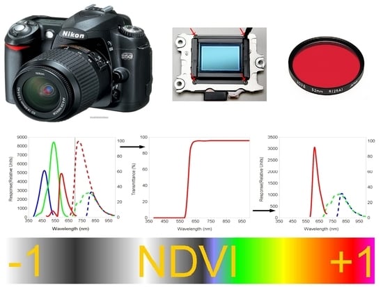
For the extraction of the hot mirror in the Nikon D50 camera we follow the tutorial of Lifepixel (http://www.lifepixel.com/tutorials/infrared-diy-tutorials/nikon-d50). The battery of the camera was removed a week before the extraction to avoid damage in the electronic circuits by static electricity. The hot-mirror was substituted by a thin piece of transparent glass of the same dimensions that protects the sensor from dust accumulation. The D50 is then transformed into a full-spectrum device that detects UV, RGB and NIR wavelengths (Figure 1, left). However, the photometer cannot be used because the piezoelectric functionality has been lost with the extraction of the hot-mirror. Consequently, as the full-spectrum camera receives now a higher light intensity, the photographs must be taken in manual mode. This requires modification of the F-spot and shutter speed and the checking of exposure histogram. In practice, this method needs different trials to find the correct range of exposures (Table 1).
2.2. Filters Used for the Simultaneous Detection of R and NIR Wavelengths
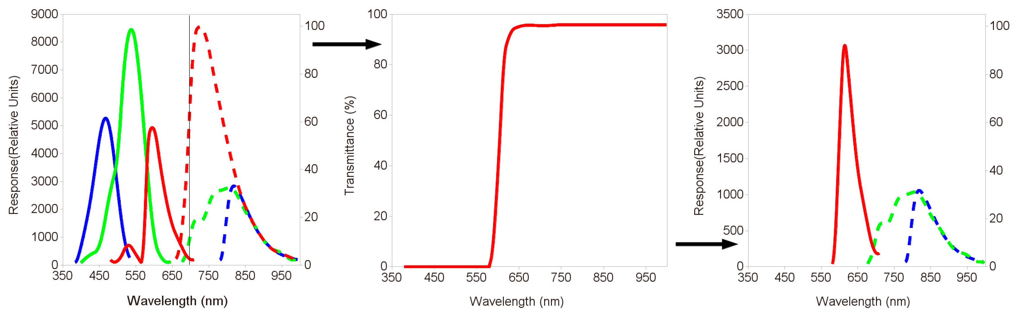
After the preliminary tests with different R (Wratten Number 25) filters, we decided to use the Hoya A25 R filter by its quality and performance. This company indicates the 95% of transmittance occurs between R and NIR wavelengths cutting off the rest of radiations (Figure 1, center). This permits to achieve a perfect discrimination between R and NIR radiations for photosynthetic analysis [20]. However, at the beginning of the R band the percentage of transmittance is smaller. With the A25 filter in the full-spectrum camera the G and B sensors can measure NIR radiation because G and B wavelengths have been completely blocked and the internal hot filter extracted. We analyze the overlap between the filter and the full-spectrum camera wavelengths [22], obtaining the final transmittances measured by the sensor (Figure 1, right). Previous studies under the same experimental conditions, show that the G channel captures the NIR light over 700 nm (NIR1), whereas the B channel detects the NIR radiation over 800 nm (NIR2) [25,26].
2.3. Covering the Maximum Possible Variability in the Photographs
The experimental conditions of the full-spectrum camera for the determination of NDVI have been broad enough to be used in natural environments. Throughout each day, the relative proportion of the red and infrared light changes so that enough hours were covered (Table 1). The NDVI photograph can be taken on specific landscapes or plants, so a sufficiently wide range of focal lengths (27–72 mm) was registered too. One of the most important aspects in our NDVI methodology is the control of the exposure, since this allows to block the excess of red radiation in central hours of the day or on the contrary, to open the entrance of infrared radiation at dawn and dusk. For all these reasons, the highest possible exposure conditions were covered.
If we want our methodology to be applied in real conditions, we must take into account that the spectral composition of light can oscillate greatly with different characteristics of the adjacent vegetation [27]. Each plant species intercept to a greater or lesser extent certain wavelengths, leaving the rest as reflected radiation. Therefore, it is not the same to take a photograph under a dense forest than a sparse one. The spectral composition could also vary depending on whether the forest is coniferous or deciduous. Other factors that can greatly affect the spectral characteristics of an area are leaf morphology, leaf water content, or leaf chemical composition [27].
For all these reasons, we decided to include photographs taken both in the open field and under the tops of various urban trees. However, we have not considered independently testing the effect of these factors, as they are included in the general variability of diaphragm apertures and shooting speeds.
2.4. Weighting the RGB Channels in Each Light Condition
Any digital camera is going to measure brightness on its RGB channels. These can vary greatly depending on the incident lighting conditions. Therefore, it is necessary to balance the range of variability of these radiations previously to each photograph [28]. Also, the ratio between NIR1 and NIR2 can be affected by factors associated with climatic conditions and landscape characteristics [6]. Moreover, for the determination of NDVI we must register the R and NIR reflectances that are defined as the ratio between the incident radiation and the reflected brightness [20]. Finally, we must bear in mind that R radiation decreases at dawn and dusk with respect to the NIR1 and NIR2.
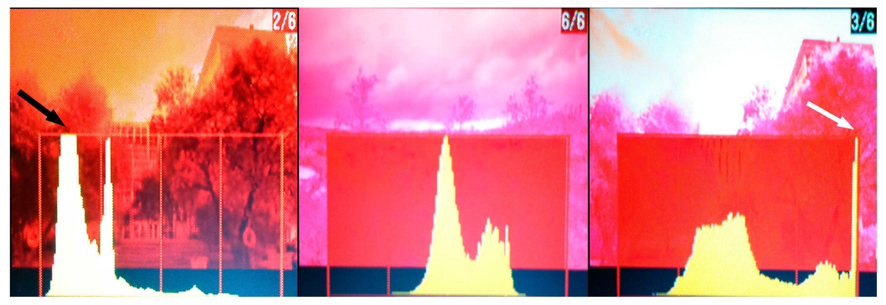
To solve all these issues, we carried out 23 tests based on photographs using a color checker at different times of the day and at different focal distances, exposures, and F-stop and shutter speeds (Table 1). The 23 photographs were taken by placing the Macbeth ColorChecker (11 inches by 8.25 inches) on the ground facing an incident light to avoid any shadows and at a distance of 1 m. The ranges of the different radiations must be equalized and this requires the use of a manual method called Custom White Balance (CWB). In the CWB procedure, we take a completely overexposed photograph per trial, by focusing the camera towards the sky for almost 30 s at the maximum diaphragm aperture (4.5 of F-stop in the Nikon D50). This photograph is used as a reference because it has the same maximum brightness in the three channels (R, NIR1 and NIR2) for the special light conditions at each moment. In consequence, we adapt the camera to the relative proportions of R, NIR1 and NIR2 previously to take the photograph. Also, CWB avoids the vignetting that is the differential brightness or saturation between the periphery and the center of the image [29]. Additionally to CWB, after each photograph we get the best results checking the appropriate range of exposure using the light intensity histograms. The photographs that showed signs of over or under exposure were rejected (Figure 2).
2.5. Use of RAW Format
In order to correct appropriately the balance and exposure, we must work in RAW format because it captures sensor data directly without any image post-processing [25]. Also, in RAW format, the relationship between the brightness and the information measured by the camera is more straightforward than with PNG or JPG formats [20]. In this sense, previous studies have shown that the Nikon D50 has an optimal linear relationship between RAW and brightness [22]. The RAW images, that in the Nikon D50 have the extension.NEF, were converted into TIFF format (consequently without post-processing) using the following command in the DCRAW 9.20 software [30]:
dcraw -v -r 1 1 1 1 -M -o 0 -q 3 -W -T -4 -g 1 1 -t 0 *.NEF
This is necessary because we use ImageJ [31] for image analysis and this software cannot use directly RAW format. Algorithm (1) transforms the exact image quantitative information into TIFF format without any changes. Also, algorithm (1) balances the R, NIR1 and NIR2 wavelengths measured by the RGB sensor, writes the output in 16 bits linear TIFF with metadata and avoids the vignetting [30]. Additionally, we developed an equalization of histograms with the following script of the ImageMagick 7.0.10 (www.imagemagick.org) software:
#!/bin/bash for f in ‘ls *.tif’; do convert $f -auto-level $f; done
This process expands the brightness range to the maximum amplitude, eliminating the exposure differences between photographs.
2.6. Using Gretag Macbeth Color Checker to Validate R and NIR Wavelengths
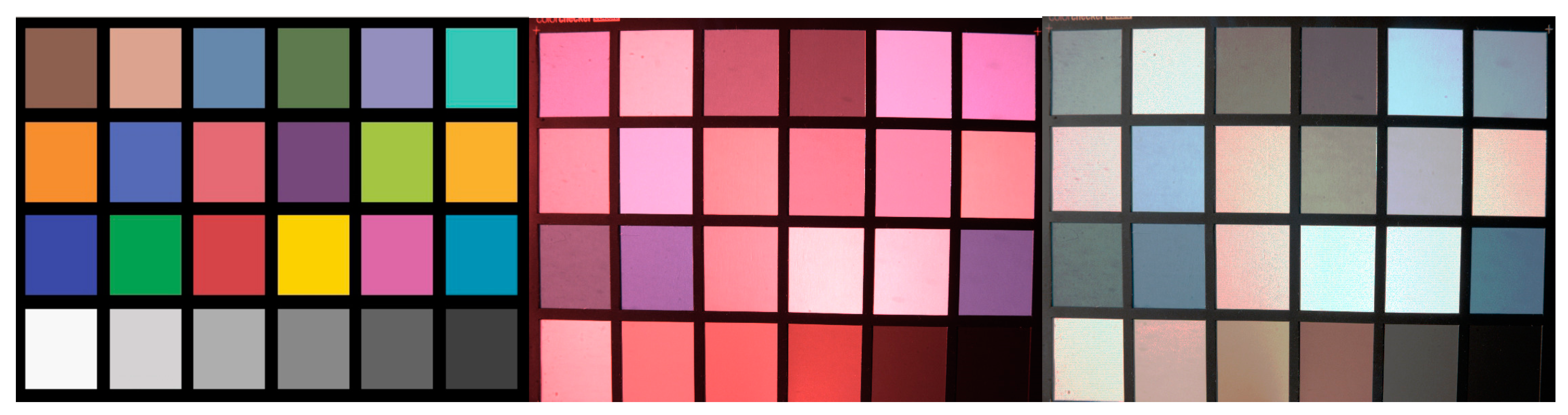
Using the CWB, the post-processing with dcraw and the histogram equalization, we have largely corrected brightness variability between photographs caused by variation in light conditions. Consequently, all the information of each photograph depends now on the variability in the photosynthetic emissions exclusively. However, the residual variability between photographs must be statistically analyzed to construct predictive regression models that relate reflectance and brightness to R and NIR1 and NIR2 radiations. In this sense, Gretag Macbeth (Figure 3) color checker is a standard color widely used for calibrating different digital image devices [28]. The detailed reflectance information on this standard has been previously published for visible (RGB) and NIR wavelengths [21] and they are supplied by the manufacturer, and therefore clearly the same for all Macbeth ColorChecker devices as they are factory calibrated.
2.7. Statistical Analysis of Reflectance-Brightness Relationship for R and NIR Wavelengths
Each one of the RGB brightness values of the 24 panels of the Gretag Macbeth color chart were measured for different trials (Table 1) using ImageJ 1.8.0 software [31]. All trials were conducted between April and June 2019 in the city of Cáceres (Spain). The ISO sensitivity was not modified in these tests and was kept as low as possible (200 ASA) to avoid the risk of overexposure, much higher in a full spectrum chamber due to the extraction of the hot mirror.
We estimate three regression models between RGB brightness (independent terms) and R, NIR1 and NIR2 reflectances (dependent terms) using the R statistical environment [32] (Table 2). The models were tested according to different statistical parameters such as R2 values, F-ratio of ANOVA test, significance and standard error of coefficients, residual normality and heteroscedasticity [33]. The residuals of these models with respect to the different factors of variation such as daytime, focal length, F-stop and shutter speed were tested using a Hierarchical Partitioning (HP) test using the hiert.part [34] library in R statistical environment. HP has been widely employed for data that does not meet the statistical requirements of parametric variance analysis that are residuals normality and variance homogeneity [35]. HP analysis shows the percentages of independent effect of each factor on the residuals of the dependent variable using a randomization test. Once we determined which factors show a significant effect (Table 3), we restricted the regression analysis to the range of conditions where our camera can be employed with success for NDVI analysis (Table 1). Finally, the coefficients of these regressions were used in a script for ImageJ (Appendix A). This allows a fast calculation of NDVI values in any photograph with the full-spectrum camera and red filter.
All statistical calculations and image processing were performed on a machine with the Debian 10.0 GNU Linux version.
3. Results
We have found that apertures of less than 6.1 markedly overexposed the images and above 14.3 it is impossible to capture enough infrared radiation and NDVI estimates were incorrect. In fact, the observed range of appropriate exposures (6.1 to 14.3) is specific to this camera model and may vary in others (Table 1). Due to hot-mirror filter removal, manual exposure control of Nikon D50 requires some trials to ensure a correct brightness histogram (Figure 2). The best conditions of shooting were also determined by the central position of the histograms, without under-exposure (Figure 2, left) or over-exposure (Figure 2, right). The most appropriate shooting speeds were between 1/6 and 1/500 s. Faster speeds do not allow enough infrared radiation and lower speeds overexpose the image. Therefore, our results strongly support the use of CWB and histogram equalization techniques as appropriate methodologies for controlling the adequate exposure and shooting speeds under the range of experimental conditions tested in Table 1. However, our method requires some prior testing due to filter removal, as the camera cannot act in automatic mode.
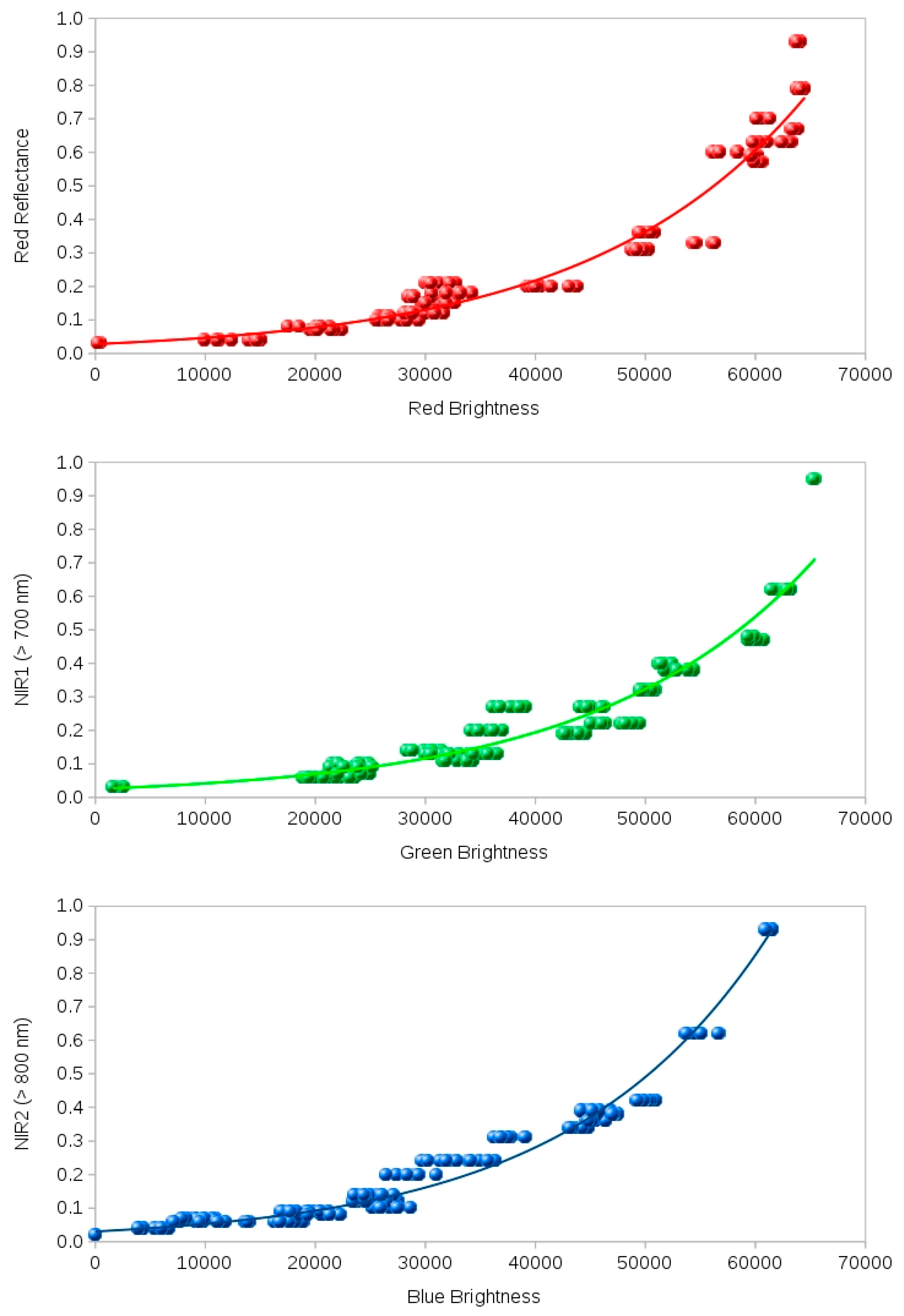
Importantly, the range of reflectance and brightness tested in the camera is as wide as possible from the red and infrared channels. Our results show that the estimation of NDVI can be made for any value of these parameters, since technically finding a perfect reflectance of 1.0 is practically impossible (Table 1). On the basis of 552 data (23 photographs), the three exponential regression models were adjusted between the reflectance of the RGB channels of the 24 color checker panels and their brightness. These models gave very high and significant adjustments, especially the red channel (Figure 3 and Table 2) with an R2 of 0.953. Also, a maximum significance according to the Student t-test for the constant and the coefficient of the independent term is observed. With this fitting, we can infer that the red reflectance is formed only by red light because this wavelength is not cut by the Hoya A25 filter and saturates the red sensors. Also, the filtering discarded any interference between R and NIR radiations because this last one is much less abundant. With regard to relationships between NIR1 wavelengths (over 700 nm) and G channel of the camera, we observe a high fit too (R2 = 0.952) (Figure 3, Table 2). Therefore, NIR1 reflectance (>700 nm) can be perfectly inferred using G brightness measurements. In this case, any interference of red light is impossible because this radiation is fully included within the red channel. At this stage of the process, an appropriate CWB is required to avoid that photographs can be overexposed by an excess of red light (not absorbed by the sensor) that is much more abundant than any type of infrared light. Also, we must discard any influence of the green light because it is completely cut off by the A25 filter. Therefore, green tones in the image only can correspond to NIR1 wavelengths. Finally, regression equation for B radiation is significant enough (R2 = 0.847) to measure NIR2 (over 800 nm) wavelengths. This light is much less abundant that NIR1 and the only possible problem could be the infra-exposure, but this is newly controlled by the CWB and brightness histogram (Figure 2). Also, NIR2 is far from the peak emissions of chlorophyll (Figure 1) and consequently it is not relevant for NDVI determination. Therefore, our results indicate that it is perfectly possible to estimate the NDVI value using the red and green colors of the image. This corresponds (when the regression equations are used) to the red and NIR1 reflectance. Although the equations are sufficient to estimate the NDVI value, it is conceptually important to determine whether the residues of the regressions (differences between observed and expected values) are influenced by the experimental conditions. In this sense, the hierarchical partitioning (HP) analysis clearly shows that any of the experimental factors (time of the day, focal length, f-stop and shooting speed) is significant (Table 3). In addition, we can observe that in the color checker, the 24 panels perfectly collect the RGB (Figure 4, top), R-NIR1-NIR2 brightness (Figure 4, center) and the corresponding reflectance determined by regressions (Figure 4, bottom).
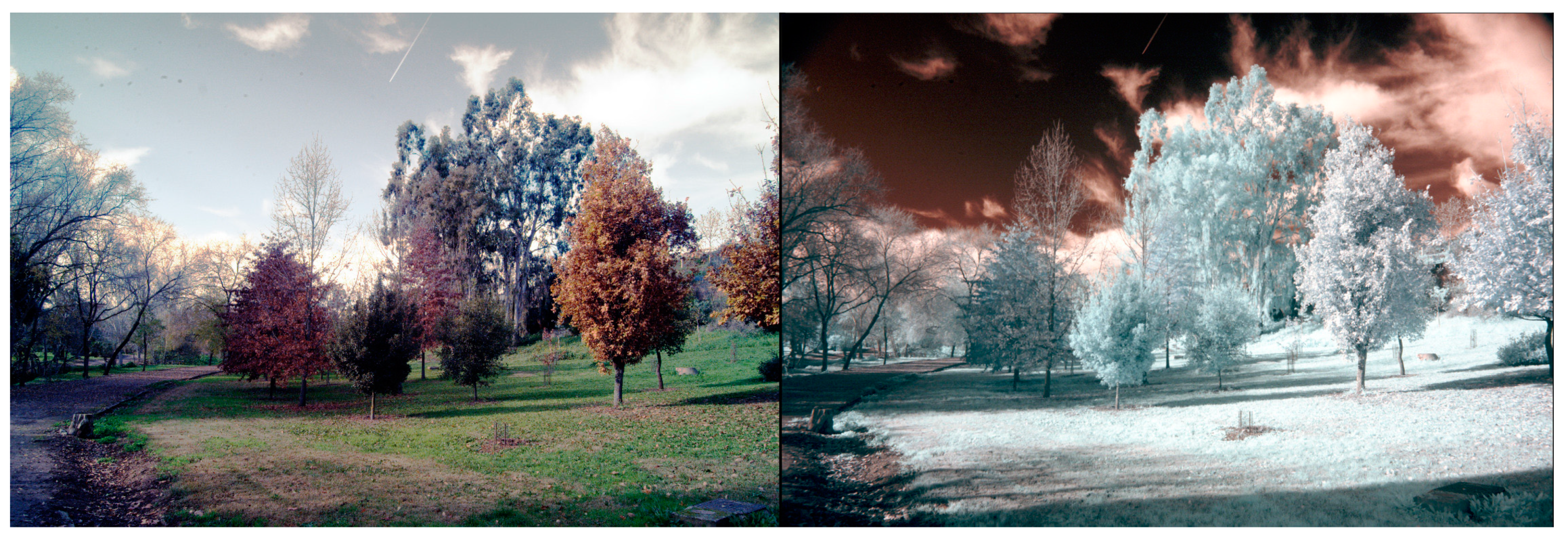
Therefore, proposed calibration equations are reliable along the tested intervals that are wide enough to apply them in natural situations. In this regard, an urban garden at the beginning of the spring can be ideal for testing our full spectrum camera by the high variability of plants and artificial surfaces. In the RGB image, the leaves of grass and trees show different tones of green color. However, using the full-spectrum camera with Hoya A25 filter, we have acquired a R-NIR image where it is possible to observe large differences between species (Figure 5). The intense infrared emission of a Eucalyptus camaldulensis (Dehnh) tree can be observed in a second plane of the Figure 5. In contrast, the Quercus petraea (Matt) tree in the center-right of the image, shows less emission. In other more complex area of the same urban park and when the script of Appendix A is used, the positive values of NDVI appear in different colors whereas the negative values are shown in gray tones (Figure 6).
Negative NDVI values from black to white correspond to water, soil, sky and trunks as expected from non-photosynthetic materials. In contrast, the high emissions of grass (in G) and the small shrubs close to the water (Ligustrum vulgare, L.) (in R) are highlighted. Trees in Figure 6 are Populus nigra L. with partially formed leaves that do not cover the canopy. Their NDVI values are medium with green tones. In this image, it is also possible to detect differences between dry (left) and wet (right) grass areas, and also the slight NDVI values (in blue) observed in lichens (trunks) and algae (water).
4. Discussion
Using a conventional digital camera to estimate the NDVI value has multiple advantages. Firstly, a significant reduction in cost, since the cameras to estimate NDVI tend to be very expensive. Lately, cheaper models of NDVI cameras are appearing on the market (i.e., MAPIR Survey3W, AgroCam or MaxMax cameras), although adapting an old camera is even more affordable. It also allows us a high image quality because the resolution is usually quite high. In this sense, the use of conventional cameras to estimate NDVI values allows determining photosynthetic variations in highly complex environments such as natural or urban areas. Also, a conventional satellite image does not allow to appreciate details so clearly as a digital camera in the terrain. Another advantage of the use of conventional digital cameras is that the R2 coefficients in R, NIR1 and NIR2 are higher (Table 2) than those observed in other studies using remote sensing on satellite imagery [8]. Moreover, our estimations are close to those obtained using spectrophotometers [20], whose calibration is time consuming [29]. In other words, we have the reliability of a laboratory device for estimating NDVI values in natural situations. Previously, we had demonstrated that it is not necessary the use of two cameras for NDVI determination [21]. Finally, the possibility of estimating with accuracy parameters as NDVI allows incorporation of this information to GIS systems or calibration of remote sensing data. These are fundamental necessities in geotechnologies [36].
Despite all these advantages, the use of digital cameras to estimate the NDVI value poses some difficulties. The first one is to remove the hot-mirror filter and replace it with a clear glass. In this sense, in the most modern digital cameras this filter is welded so it cannot be easily removed. The Nikon D50 does not pose any difficulties with this aspect and the web tutorials are very easy to apply. Although the Nikon D50 has not been manufactured for decades, it can easily be purchased second-hand in virtual stores such as eBay, Amazon or AllExpress. If someone would like to use another model, it is possible to adapt the proposed methodology to other digital cameras as long as the hot mirror can be extracted and they use RAW format. Another difficulty in the use of full-spectrum cameras for NDVI determination is shooting in the manual mode. This requires some previous tests to delimit the ideal conditions in each case. Here, we show a wide range of experimental conditions that demonstrate that our methodology can be applied in very different situations of natural environments.
Our method is progressive and covers different methodological steps that are not difficult to implement, including the use of RAW format, the CWB previous to each set of photographs, the control of exposure by brightness histogram, the equalization and the use of a script in ImageJ for the determination of NDVI values in an appropriate color scale. This protocol must be carefully followed because it is a manual process that requires certain ability with digital cameras. The first step is the use of a RAW format that requires acquisition of cameras of a certain level. A priori, our procedure does not exclude the use of other formats (JPG or PNG) although we believe that the calibrations would be much worse because linearity between input and output of the sensor is lost. The second methodological step, the determination of the custom white balance (CWB), it is more complex as it requires adapting the camera to the light conditions of each moment. Definitely, this step is very delicate, since having removed the hot-mirror filter the possibility that the red light completely saturates all the channels is elevated. Therefore, the image must be overexposed by balancing the three channels and the exposure must be carefully controlled by means of the intensity histogram. Obviously, it has to be done in manual mode and after several tests with different shooting speeds and diaphragms until the right conditions are found. With practice a few tests are sufficient. We must bear in mind that light conditions can vary in minutes due to factors such as variable cloud cover or if we are under the top of a tree. If conditions are stable, such as on a cloudless or completely cloudy day, the same CWB may serve for a certain time. Finally, we must transform the brightness values of the red and green channels to red and infrared (NIR1) reflectances using appropriate regression models. As expected, these equations vary with the camera model because they are related to the algorithms of adaptation between brightness received and stored in the image. Once established these regressions, can be applied to for all the individual cameras of the same model. Consequently, the equations in this research are valid for all the Nikon D50 cameras but must be calculated for other models. The high adjustments observed in our regressions and above all, the lack of significance of the residues from any of the experimental factors, give us guarantees that these equations are usable in all the tested range of conditions. Therefore, our procedure allows the analysis of the red-edge defined as the area of transition between R and NIR1 wavelengths (Figure 1). Red-edge corresponds to the maximum chlorophyll fluorescence emission [3]. Even the blue channel, that recovers the infrared light NIR2, could be used with our methodology, although this light has no functional significance in photosynthesis. These final stages can be completely automatized using the proposed script, which can be applied to thousands of photographs in few minutes. Obviously, the script must be adapted to each camera with the appropriate calibrations between reflectance and brightness, using the Gretag Macbeth color checker or other equivalent. Only this step varies among cameras, whereas the previous procedures are common to all the models.
In NDVI analysis of landscapes different satellite images (LANDSAT, WorldView, GeoEye…) of few meter resolutions are usually employed [36]. Our method offers even a higher level of resolution (5 Mp in Nikon D50) allowing a detailed analysis of NDVI variability. Therefore, it opens the possibility of future uses of this type of modified digital cameras coupled on drones for landscape studies [24]. Other procedures using two or three cameras requires more sophisticated airborne devices as hot air balloons or airplanes [29]. Another advantage of our methodology is that it allows the NDVI analysis in spatially complex environments as are observed in urban areas. Additionally, our methodology can be easily applied to remote sensing in very fragmented areas, where can appears problems of differentiation to medium or low resolutions between pixels of adjacent structures (-i.e., green and building areas). This is known as the mixed pixel problem [36]. In fact, our method discriminates between living and non-living structures which are neatly differentiated by its NDVI values. Besides, NDVI values of the observed plant species and abiotic areas are congruent with our previous information on the area, plant phenology and seasonal conditions. Another important application of our method of NDVI stimation, is in multivariate approaches with others variables used in remote sensing such as greenness, redness or plant senescence [37]. In summary, our procedure can be easily adapted to any type of digital camera that allows both storing of digital information in RAW format and an easy extraction of the hot-mirror, provided that equations vary according to brightness-reflectance relationships specific of each type of camera. We propose a valuable and useful procedure to adapt conventional digital cameras to NDVI analysis.
5. Conclusions
The present work shows that it is possible to determine the NDVI parameter with a digital camera model, the Nikon D50. The procedure consists of steps that can be adapted to any camera such as extraction of the hot-mirror filter, use of white balance, calibration with color chart, normalization of images and use of the prediction equations. Our method is much simpler than others previously used that require several images or several cameras, since one single image allows estimation of the NDVI value. In addition, the proposed method gives notoriously higher determination coefficients than many previous researches that use satellite images. Being the resolution higher than any satellite image we can determine species changes at very small scales. This opens enormous possibilities of application in urban ecology studies where both fragmentation of the landscape and complexity of distribution of plant species tend to detract from clear photosynthetic analysis. Although, more tests with more camera models are required, an important advantage of the proposed methodology is that it can be applied by amateur scientists and photography enthusiasts in general.
Funding
This research received no external funding.
Acknowledgments
We thank Reto Stöckli from the Federal Office of Meteorology and Climatology MeteoSwiss, Zurich, Switzerland for the papers that inspired our work and his useful suggestions. We also want to thank Francisco Miguel Martínez Verdú for giving us the basic information about the general theory of color and white balance in RGB cameras. Germán Larriba made important observations on the manuscript. We would also like to thank other scientists that are cited in the references by their useful contribution to this area of research. This work would not have been possible without the detailed information provided by Nikon and LifePixel. We thank Graeme Henshall from Mortimer SL translation company for the English style review.
Conflicts of Interest
The authors declare no conflict of interest.
Appendix A
Script in ImageJ for NDVI analysis of full-spectrum images with Red Filters.
Run(“32-bit”);
saveAs(“Tiff”, “/tmp/test.tif”);
run(“Split Channels”);
selectWindow(“C3-test.tif”);
run(“Close”);
selectWindow(“C1-test.tif”);
run(“Multiply...”, “value=0.0000573”);
run(“Exp”);
run(“Multiply...”, “value=0.0235”);
saveAs(“Tiff”, “/tmp/R.tif”);
selectWindow(“C2-test.tif”);
run(“Multiply...”, “value=0.0000561”);
run(“Exp”);
run(“Multiply...”, “value=0.0307”);
saveAs(“Tiff”, “/tmp/IR1.tif”);
imageCalculator(“Subtract create 32-bit”, “IR1.tif”,”R.tif”);
saveAs(“Tiff”, “/tmp/N1.tif”);
imageCalculator(“Add create 32-bit”, “IR1.tif”,”R.tif”);
saveAs(“Tiff”, “/tmp/D1.tif”);
selectWindow(“R.tif”);
close();
selectWindow(“IR1.tif”);
close();
imageCalculator(“Divide create 32-bit”, “N1.tif”,”D1.tif”);
selectWindow(“Result of N1.tif”);
run(“NDVI_colors”);
saveAs(“Tiff”, “/tmp/NDVI.tif”);
selectWindow(“D1.tif”);
close();
selectWindow(“N1.tif”);
close();
References
- Ritchter, M.; Weiland, U. Applied Urban Ecology: A Global Framework; Blackwell Publishing: West Sussex, UK, 2012. [Google Scholar]
- Rouse, J.W., Jr.; Haas, R.H.; Deering, D.W.; Schell, J.A.; Harlan, J.C. Monitoring the Vernal Advancement and Retrogradation (Green Wave Effect) of Natural Vegetation; NASA/GSFC Type III Final Report; National Aeronautics and Space Administration NASA: Greenbelt, MD, USA, 1974. [Google Scholar]
- Maxwell, K.; Johnson, G.N. Chlorophyll fluorescence. A practical guide. J. Exp. Botany 2000, 51, 659–668. [Google Scholar] [CrossRef]
- Silleos, N.G.; Alexandridis, T.K.; Gitas, I.Z.; Perakis, K. Vegetation indices: Advances made in biomass estimation and vegetation monitoring in the last 30 years. Geocarto Int. 2006, 21, 21–28. [Google Scholar] [CrossRef]
- Rocha, A.V.; Shaver, G.R. Advantages of a two band EVI calculated from solar and photosynthetically active radiation fluxes. Agric. For. Meteorol. 2009, 149, 1560–1563. [Google Scholar] [CrossRef]
- Matsushita, B.; Yang, W.; Chen, J.; Onda, Y.; Qiu, G. Sensitivity of the enhanced vegetation index (EVI) and normalized difference vegetation index (NDVI) to topographic effects: A case study in high-density cypress forest. Sensors 2007, 7, 2636–2651. [Google Scholar] [CrossRef] [PubMed] [Green Version]
- Meng, Q.; Cieszewski, C.J.; Madden, M.; Borders, B. A linear mixed-effects model of biomass and volume of trees using Landsat ETM+ images. For. Ecol. Manag. 2007, 244, 93–101. [Google Scholar] [CrossRef]
- Flowers, M.; Weisz, R.; Heiniger, R. Quantitative approaches for using color infrared photography for assessing in-season nitrogen status in winter wheat. Agron. J. 2003, 95, 1189–1200. [Google Scholar] [CrossRef] [Green Version]
- Li, R.H.; Li, X.B.; Li, G.Q.; Wen, W.Y. Simulation of soil nitrogen storage of the typical steppe with the DNDC model: A case study in Inner Mongolia, China. Ecol. Indic. 2014, 41, 155–164. [Google Scholar] [CrossRef]
- Szilagyi, J.; Parlange, M.B. Defining watershed-scale evaporation using a normalized difference vegetation index. J. Am. Water Resour. Assoc. 1999, 35, 1245–1255. [Google Scholar] [CrossRef]
- Martínez, B.; Gilabert, M.A. Vegetation dynamics from NDVI time series analysis using the wavelet transform. Remote Sens. Environ. 2009, 113, 1823–1842. [Google Scholar] [CrossRef]
- He, Y.; Bo, Y.; De Jong, R.; Li, A.; Zhu, Y.; Cheng, J. Comparison of vegetation phenological metrics extracted from GIMMS NDVIg and MERIS MTCI data sets over China. Int. J. Remote Sens. 2015, 36, 300–317. [Google Scholar] [CrossRef]
- Lloret, F.; Lobo, A.; Estevan, H.; Maisongrande, P.; Vayreda, J.; Terradas, J. Woody plant richness and NDVI response to drought events in Catalonian (Northeastern Spain) forests. Ecology 2007, 88, 2270–2279. [Google Scholar] [CrossRef] [PubMed]
- Jafari, R.; Lewis, M.M.; Ostendorf, B. An image-based diversity index for assessing land degradation in an arid environment in South Australia. J. Arid Environ. 2008, 72, 1282–1293. [Google Scholar] [CrossRef]
- Maselli, F.; Romanelli, E.; Bottai, L.; Zipoli, G. Use of NOAA-AVHRR NDVI images for the estimation of dynamic fire risk in Mediterranean areas. Remote Sens. Environ. 2003, 86, 187–197. [Google Scholar] [CrossRef]
- Bacaro, G.; Santi, E.; Rocchini, D.; Pezzo, F.; Puglisi, L.; Chiarucci, A. Geostatistical modelling of regional bird species richness: Exploring environmental proxies for conservation purpose. Biodivers. Conserv. 2011, 20, 1677–1694. [Google Scholar] [CrossRef]
- Murphy, R.J.; Underwood, A.J. Novel use of digital colour-infrared imagery to test hypotheses about grazing by intertidal herbivorous gastropods. J. Exp. Mar. Biol. Ecol. 2006, 330, 437–447. [Google Scholar] [CrossRef]
- Oesterheld, M.; DiBella, C.M.; Kerdiles, H. Relation between NOAA-AVHRR Satellite Data and Stocking Rate of Rangelands. Ecol. Appl. 1998, 8, 207–212. [Google Scholar] [CrossRef]
- Thanapura, P.; Helder, D.L.; Burckhard, S.; Warmath, E.; O’Neill, M.; Galster, D. Mapping urban land cover using Quickbird NDVI and GIS spatial modelling for runoff coefficient determination. Photogramm. Eng. Remote Sens. 2007, 73, 57–65. [Google Scholar] [CrossRef] [Green Version]
- Rabatel, G.; Gorretta, N.; Labbé, S. Getting simultaneous red and near-infrared band data from a single digital camera for plant monitoring applications: Theoretical and practical study. Biosyst. Eng. 2014, 117, 2–14. [Google Scholar] [CrossRef] [Green Version]
- Ritchie, G.L.; Sullivan, D.G.; Perry, C.D.; Hook, J.E.; Bednarz, C.W. Preparation of a low-cost digital camera system for remote sensing. Appl. Eng. Agric. 2008, 24, 885–896. [Google Scholar] [CrossRef]
- Verhoeven, G.J.; Smet, P.F.; Poelman, D.; Vermeulen, F. Spectral characterization of a digital still camera’s NIR modification to enhance archaeological observation. IEEE Trans. Geosci. Remote Sens. 2009, 47, 3456–3468. [Google Scholar] [CrossRef]
- Weekley, J.G. Multispectral Imaging Techniques for Monitoring Vegetative Growth and Health. Master’s Thesis, Virginia Polytechnic Institute, Blacksburg, VA, USA, 2007. [Google Scholar]
- Yang, C.; Everitt, J.H.; Davis, M.R. A CCD camera-based hyperspectral imaging system for stationary and airborne applications. Geocarto Int. 2003, 18, 71–80. [Google Scholar] [CrossRef]
- Verhoeven, G.J. Becoming a NIR-sensitive aerial archaeologist. In Remote Sensing for Agriculture, Ecosystems, and Hydrology IX; Neale, C., Owe, M., D’Urso, G., Eds.; SPIE: Bellingham, WA, USA; Florence, Italy, 2007; pp. 333–345. [Google Scholar]
- Verhoeven, G.J. Near-infrared aerial crop mark archaeology: From its historical use to current digital implementations. J. Archaeol. Method Theory 2012, 19, 132–160. [Google Scholar] [CrossRef]
- Homolová, L.; Maenovsky, Z.; Clevers, J.G.P.W.; García-Santos, G.; Schaeprnan, M.E. Review of optical-based remote sensing for plant trait mapping. Ecol. Complex. 2013, 15, 1–16. [Google Scholar] [CrossRef] [Green Version]
- Martínez-Verdú, F.; Pujol, J.; Capilla, P. Characterization of a digital camera as an absolute tristimulus. J. Imaging Sci. Technol. 2003, 47, 279–374. [Google Scholar]
- Lebourgeois, V.; Bégué, A.; Labbé, S.; Mallavan, B.; Prévot, L.; Roux, B. Can commercial digital cameras be used as multispectral sensors? A crop monitoring test. Sensors 2008, 8, 7300–7322. [Google Scholar] [CrossRef] [PubMed]
- Russell, J.; Cohn, R. Dcraw; Book on Demand Ltd.: Miami, FL, USA, 2012. [Google Scholar]
- Schneider, C.A.; Rasband, W.S.; Eliceiri, K.W. NIH image to ImageJ: 25 years of image analysis. Nat. Methods 2012, 9, 671–675. [Google Scholar] [CrossRef]
- R: A Language and Environment for Statistical Computing. Available online: https://www.R-project.org/ (accessed on 5 October 2020).
- Jobson, J.D. Applied Multivariate Data Analysis, 4th ed.; Springer: New York, NY, USA, 1991. [Google Scholar]
- Hier.part: Hierarchical Partitioning. Available online: http://cran.R-project.org/package=hier.part (accessed on 21 May 2019).
- Chevan, A.; Sutherland, M. Hierarchical partitioning. Am. Stat. 1991, 45, 90–96. [Google Scholar]
- Boyd, D.S.; Foody, G.M. An overview of recent remote sensing and GIS based research in ecological informatics. Ecol. Inform. 2011, 6, 25–36. [Google Scholar] [CrossRef] [Green Version]
- Zhao, J.; Zhang, Y.; Tan, Z.; Song, Q.; Liang, N.; Yu, L.; Zhao, J. Using digital cameras for comparative phenological monitoring in an evergreen broad-leaved forest and a seasonal rain forest. Ecol. Inform. 2012, 10, 65–72. [Google Scholar] [CrossRef]
Figure 1.
Functionality of Nikon D50 full-spectrum with Hoya A25 red filter. (Left): Spectral response of camera without filter in visible (continuous lines) and infrared wavelengths (discontinuous lines). The response of the camera in the visible wavelengths is 100 times more intense. (Center): Transmittance of Hoya A25 filter. (Right): Final response of the camera. Blue and green visible lights had been eliminated by the filter, leading green and blue cells of the sensor free. The red channel is filled by red light that is more abundant (100×). Green channel capture the infrared light over 700 nm. Blue channel displays the infrared light over 800 nm.

Figure 2.
Histograms of exposure. (Left): underexposed (black arrow). (Center): correctly exposed. (Right): overexposed (white arrow).
Figure 2.
Histograms of exposure. (Left): underexposed (black arrow). (Center): correctly exposed. (Right): overexposed (white arrow).

Figure 3.
Macbeth Gretag color checker. (Left): original image in visible wavelengths. (Center): image under red and infrared lights. (Right): after equalization, the three channels R (red), G (infrared over 700 nm, IR1) and B (infrared over 800 nm, IR2) are equilibrated in exposures.
Figure 3.
Macbeth Gretag color checker. (Left): original image in visible wavelengths. (Center): image under red and infrared lights. (Right): after equalization, the three channels R (red), G (infrared over 700 nm, IR1) and B (infrared over 800 nm, IR2) are equilibrated in exposures.

Figure 4.
Exponential regression fit between brightness (B) and reflectance (R) of a Nikon D50 full-spectrum with A25 (red) Hoya filter. (Top): Red channel captures red radiation. (Center): Green channel captures the infrared radiation between 700 and 800 nm. (Bottom): Blue channel captures the infrared wavelengths over 800 nm.

Figure 5.
Images in visible (left) and infrared (right) wavelenghts. The first image has been acquired with a conventional camera with hot-mirror filter. The second image is the result of equalization of a photography taken with the Nikon D50 full-spectrum with A25 Hoya red filter.
Figure 5.
Images in visible (left) and infrared (right) wavelenghts. The first image has been acquired with a conventional camera with hot-mirror filter. The second image is the result of equalization of a photography taken with the Nikon D50 full-spectrum with A25 Hoya red filter.

Figure 6.
Result of processing of an equalized image with conventional NDVI colors in ImageJ. In non-colored tones the NDVI values under 0 (water, soil, trunks, sky, clouds) since black (low, close to −1) to white (high, close to zero). In colored tones the values of NDVI over 0 since blue (low, close to zero) to green-yellow (medium, close to 0.5) and red (high, close to 1). The photograph correspond to an area of Prince’s Park in the city of Cáceres (SW Spain) during late summer. In the image can be seen some structures. (1) The extreme of branchs of certain high trees (Populus nigra) have not leaves due to an intense hot. (2) More resistant trees have leaves. The grass show different phenological stages since dry (3) to green (4). The values of NDVI are low in algae (5) and lichens (6) and high in certain shrubs (7).


Table 1.
Range of experimental conditions tested in this work.
| Parameter | Range |
|---|---|
| Number of photographs | 23 |
| Time | 10 a.m.–18 p.m. |
| Focal distance | 27–72 mm |
| Exposure (Ev) | 6.1–14.3 |
| F-stop | 4.5–20.0 |
| Speed | 0.002–0.17 |
| Red reflectance | 0.03–0.93 |
| Red brightness (16 bits) | 681–65,007 |
| Infrared reflectance | 0.03–0.92 |
| Infrared brightness (16 bits) | 724–65,074 |
Table 2.
Models (FM) of exponential regressions between RGB brightness (Br) and reflectances (Rf) for red (R), infrared over 700 nm (NIR1) and infrared over 800 nm (NIR2).
Table 2.
Models (FM) of exponential regressions between RGB brightness (Br) and reflectances (Rf) for red (R), infrared over 700 nm (NIR1) and infrared over 800 nm (NIR2).
| Parameters | R Reflectance~R Brightness | NIR1 Reflectance~G Brightness | NIR2 Reflectance~B Brightness |
|---|---|---|---|
| R = a*exp(b*B) | Rf = 2.35 × 10⁻² × exp(5.73 × 10⁻⁵ × Br) | Rf = 3.07 × 10⁻² × exp(5.61 × 10⁻⁵ × Br) | Rf = 5.29 × 10⁻² × exp(4.81 × 10⁻⁵ × Br) |
| Standard error (a/b) | 3.01 × 10⁻¹/6.83 × 10−7 | 3.02 × 10⁻²/6.75 × 10−7 | 5.13 × 10⁻²/1.09 × 10−6 |
| t-value (a/b) | −124.79 ***/83.92 *** | −115.36 ***/83.01 *** | −57.34 ***/43.94 *** |
| R2 | 0.953 | 0.952 | 0.847 |
***: p-value < 0.001.
Table 3.
Percentage of variance of each photographic parameter on residuals of the three initial regressions (all data) determined by Hierarchical Partitioning test; ns: non-significant effect.
Table 3.
Percentage of variance of each photographic parameter on residuals of the three initial regressions (all data) determined by Hierarchical Partitioning test; ns: non-significant effect.
| Parameter | R Brightness | G Brightness | B Brightness |
|---|---|---|---|
| Time | 31.74 ns | 42.32 ns | 59.06 ns |
| Focal length | 44.57 ns | 15.44 ns | 14.55 ns |
| F-stop | 10.13 ns | 21.48 ns | 11.59 ns |
| Speed | 13.56 ns | 20.77 ns | 14.80 ns |
Publisher’s Note: MDPI stays neutral with regard to jurisdictional claims in published maps and institutional affiliations. |
© 2020 by the author. Licensee MDPI, Basel, Switzerland. This article is an open access article distributed under the terms and conditions of the Creative Commons Attribution (CC BY) license (http://creativecommons.org/licenses/by/4.0/).
Share and Cite
MDPI and ACS Style
Patón, D. Normalized Difference Vegetation Index Determination in Urban Areas by Full-Spectrum Photography. Ecologies 2020, 1, 22-35. https://0-doi-org.brum.beds.ac.uk/10.3390/ecologies1010004
AMA Style
Patón D. Normalized Difference Vegetation Index Determination in Urban Areas by Full-Spectrum Photography. Ecologies. 2020; 1(1):22-35. https://0-doi-org.brum.beds.ac.uk/10.3390/ecologies1010004
Chicago/Turabian StylePatón, Daniel. 2020. "Normalized Difference Vegetation Index Determination in Urban Areas by Full-Spectrum Photography" Ecologies 1, no. 1: 22-35. https://0-doi-org.brum.beds.ac.uk/10.3390/ecologies1010004