Comparison of Direct and Adjoint k and α-Eigenfunctions

Abstract

Modal expansions based on k-eigenvalues and α-eigenvalues are commonly used in order to investigate the reactor behaviour, each with a distinct point of view: the former is related to fission generations, whereas the latter is related to time. Well-known Monte Carlo methods exist to compute the direct k or α fundamental eigenmodes, based on variants of the power iteration. The possibility of computing adjoint eigenfunctions in continuous-energy transport has been recently implemented and tested in the development version of TRIPOLI-4^®, using a modified version of the Iterated Fission Probability (IFP) method for the adjoint α calculation. In this work we present a preliminary comparison of direct and adjoint k and α eigenmodes by Monte Carlo methods, for small deviations from criticality. When the reactor is exactly critical, i.e., for k₀ = 1 or equivalently α₀ = 0, the fundamental modes of both eigenfunction bases coincide, as expected on physical grounds. However, for non-critical systems the fundamental k and α eigenmodes show significant discrepancies.

1. Introduction

Assessing the asymptotic behaviour of a nuclear system is intimately related to computing the dominant direct (Here and throughout the manuscript, the terms ‘direct’ and ‘forward’ are equivalently used.) eigenmode and the associated dominant eigenvalue of the configuration under analysis, which is central in several applications in reactor physics, including pulsed neutron reactivity measurements [1] and reactor period analysis [2,3,4]. Furthermore, for several key reactor coefficients, such as kinetics parameters, sensitivities to nuclear and material data, or perturbations [5,6,7,8,9,10], bilinear forms involving both the direct and the adjoint fundamental eigenfunctions are required. The most common bases for eigenfunction expansions are those related to the k-eigenvalues and to the α-eigenvalues, respectively [11]. Calculations of dominant k or α eigenvalues/eigenfunctions try to assess the asymptotic reactor behaviour, each with a distinct point of view: the former basically determines the shape of the neutron population after a large number of fission generations, whereas the latter after a sufficiently long time. When the reactor is exactly critical, i.e., for k₀ = 1 or equivalently α₀ = 0, the fundamental modes of both eigenfunction bases coincide, as expected on physical grounds [11]. However, for systems far from criticality the fundamental k and α eigenmodes show discrepancies and (with the possible exception of very simple cases involving single-speed transport) are not related to each other in any trivial manner [11,12]. Such discrepancies have been observed even for very small deviations from criticality [13]. Since both direct and adjoint eigenmodes are involved in the calculation of key reactor parameters, the investigation of the behaviour of the eigenfunctions might shed some light on the behaviour of such parameters at and close to the critical point.

In the context of Monte Carlo simulation, the analysis of the prompt direct fundamental k and α-eigenmodes (neglecting delayed neutron contributions) has been previously carried out for a set of sub- and super-critical systems based on homogeneous and heterogeneous cores with fast and thermal spectra [12]. In this work, we will revisit and extend these findings on some benchmark configurations, namely Godiva-like spheres inspired by the seminal work of D.E. Cullen [12] and the CROCUS core [14,15], with a twofold aim. First, we will explicitly include the effects of delayed neutrons, which have been originally neglected for the sake of simplicity. We will thus determine whether the presence of delayed contributions has an impact on the shape of the eigenfunctions, and in particular whether the discrepancies between k and α-eigenmodes increase or decrease. Then, we will examine the behaviour of the fundamental adjoint eigenmodes for both k and α-eigenvalue problems, whose comparison has not been addressed so far, to the best of our knowledge.

2. Tools and Methods

For the numerical simulations presented in the following, we have used the development version of TRIPOLI-4^® [16]. For direct k-eigenvalue calculations, the fundamental mode φ_k0 satisfying

$$L{\phi }_k\left(r,\mathsf{\Omega },E\right)=\frac{1}{k}[F_p{\phi }_k(r,\mathsf{\Omega },E)+{\displaystyle \sum _j{F}_{d,j}}{\phi }_k(r,\mathsf{\Omega },E)],$$

(1)

is computed by using the standard power iteration method [16]. Here L denotes the net loss operator, F_p the prompt fission operator, F_d,j the delayed fission operator for precursor family j, and the other notation is standard. For α-eigenvalue problems, in the form

$$\frac{\alpha }{\upsilon }{\phi }_{\alpha }\left(r,\mathsf{\Omega },E\right)+L{\phi }_{\alpha }\left(r,\mathsf{\Omega },E\right)=F_p{\phi }_{\alpha }(r,\mathsf{\Omega },E)+{\displaystyle \sum _j\frac{{\lambda }_j}{{\lambda }_j+\alpha }{F}_{d,j}}{\phi }_{\alpha }(r,\mathsf{\Omega },E)],$$

(2)

in the development version of TRIPOLI-4^® the fundamental mode φ_α0 is determined by using the α-k power iteration [17]. The α-k method was originally proposed for prompt decay constants [18] and later extended to the general case with neutrons and precursors [2,17]. The basic idea is to iteratively search for the dominant α value that makes the α-eigenvalue equation exactly critical with respect to a fictitious k-eigenvalue applied to the production terms. For positive α, a “capture” cross section α/υ is taken into account while applying a modified power iteration [12,18]. For negative α, the contribution −α/υ was originally interpreted as a “production” term [12,18]. The standard implementation of this algorithm has been however shown to be numerically unstable, possibly leading to abnormal termination: an improved algorithm that overcomes the limitations for the case of negative α has been proposed [17], introducing a special “copy” operator (at the right hand side of Equation (2)) that preserves particle balance between the power iteration cycles, namely

$$F_{\alpha }={\displaystyle \iint d}\mathsf{\Omega }’dE’\delta (\mathsf{\Omega }-\mathsf{\Omega }’)\delta (E-E’){\upsilon }_{\alpha }\frac{\left|\alpha \right|}{\upsilon (E’)’},$$

(3)

with a multiplicity υ_α = 2. The operator F_α is compensated by a “production” cross section –α/υ at the left hand side of Equation (2). The term υ_α can be interpreted as the average number of (copy) neutrons produced by the α-production operator having a delta kernel. Details concerning the implementation and the possible convergence issues for the case of negative α are provided in [17]. Finally, the term λ_j/(λ_j + α), λ_j being the decay constant for precursor family j, can be interpreted as a weight multiplier for the delayed neutron yield, observing that the dominant α satisfies α₀ > −min_jλ_j [2,17].

Concerning the adjoint k-eigenmodes ${\phi }_k^{†}$, which satisfy

$$L^{†}{\phi }_k^{†}\left(r,\mathsf{\Omega },E\right)=\frac{1}{k}[F_p^{†}{\phi }_k^{†}(r,\mathsf{\Omega },E)+{\displaystyle \sum _j{F}_{d,j}^{†}}{\phi }_k^{†}(r,\mathsf{\Omega },E)],$$

(4)

in TRIPOLI-4^® we have adopted the Iterated Fission Probability (IFP) method [19], by closely following the strategy proposed in [5,6]. The introduction of the IFP method has paved the way to obtaining the fundamental adjoint flux ${\phi }_{k_0}^{†}$ for k-eigenvalue problems in continuous-energy Monte Carlo simulations: the adjoint flux ${\phi }_{k_0}^{†}$ is equated to the neutron importance I_k, which can be then estimated by running a direct calculation [5,6]. The neutron importance I_k is obtained by recording the descendants after M latent generations for an ancestor injected into the system at coordinates r, Ω, E (neutrons are promoted to the next generation by fission events). By building upon these ideas, we have recently introduced a novel method to compute the fundamental adjoint flux ${\phi }_{{\alpha }_0}^{†}$ for α-eigenvalue problems, which solves

$$\frac{\alpha }{\upsilon }{\phi }_{\alpha }^{†}\left(r,\mathsf{\Omega },E\right)+L^{†}{\phi }_{\alpha }^{†}\left(r,\mathsf{\Omega },E\right)=F_p^{†}{\phi }_{\alpha }^{†}(r,\mathsf{\Omega },E)+{\displaystyle \sum _j\frac{{\lambda }_j}{{\lambda }_j+\alpha }{F}_{d,j}^{†}}{\phi }_{\alpha }^{†}(r,\mathsf{\Omega },E),$$

(5)

by resorting to a generalized version of IFP (G-IFP) [13]. The fundamental adjoint flux ${\phi }_{{\alpha }_0}^{†}$ can be again equated to the neutron importance I_α, i.e., can be estimated by recording the descendants after M latent generations for an ancestor injected into the system at coordinates $r,\mathsf{\Omega },E$. The only difference with respect to the regular IFP method is that for α-eigenvalue problems additional events, other than fissions, may contribute to promoting the neutrons to the next generation. For positive α, the additional term α/υ acts as a sterile capture: neutrons can thus contribute to the importance only being promoted to the next generation by prompt and delayed fission. However, for negative α, neutrons can contribute to importance also via the α-production term, associated to the copy operator with cross section −α/υ. In both cases, the weight of the delayed neutrons is assigned a correction factor ${\lambda }_j/({\lambda }_j+\alpha )$. For a thorough explanation of the G-IFP method, see [13].

3. Analysis of the Godiva-Like Spheres

In view of characterizing the behaviour of the direct and adjoint fundamental modes for k and α-eigenvalue problems, we have selected two simple benchmark configurations, both inspired from test-cases previously considered in the literature [12]. The first configuration consists in a bare sphere of uranium, whose specifications are taken from [12] (Problem I) and are very close to those of the standard Godiva benchmark [20]. In particular, the radius of the sphere is equal to 8.7407 cm and the uranium isotopic composition (normalized with respect to the uranium density) consists of 93.7695% atoms of U²³⁵, 5.2053% atoms of U²³⁸ and 1.0252% atoms of U²³⁴. The system is spatially homogeneous, and the neutron spectrum is fast. The second configuration is also taken from [12] (Problem III) and corresponds to a sphere of uranium with equal radius and uranium isotopic composition, surrounded by a thick water reflector: the system is spatially heterogeneous with a total radius of 38.7407 cm and a strong thermal component. The water density is equal to 1 g/cm³ with 2 atoms of H¹ and 1 atom of O¹⁶. For the sake of simplicity, we will call these configurations Problem I and Problem III.

3.1. Description of the Benchmark Configurations

For both cases, starting from the specifications given in [12], we have adjusted the uranium density in order to obtain slightly sub-critical and sightly super-critical configurations, with the aim of examining the effects of slight deviations from criticality on the shape of the direct and adjoint eigenmodes. The chosen values of uranium density for each configuration are shown in

Table 1. Uranium densities for benchmark configurations. Uranium isotopic mass fractions and water properties are equal to those described in the reference [12].

Configuration	ρU [g/cm3]
I sub-critical	18.6836
I super-critical	18.9085
III sub-critical	13.5676
III super-critical	13.8600

.

The simulation results displayed in the following have been obtained by resorting to TRIPOLI-4^®. The forward simulations are performed via the power iteration method for the k-eigenvalue problem, and the α-k power iteration method for the α-eigenvalue problem. The corresponding numerical simulation parameters are presented in

Table 2. Numerical simulation parameters for benchmark configurations: forward simulations.

Configuration	Active Cycles	Inactive Cycles	Particles
I sub-critical	5 × 103	103	105
I super-critical	5 × 103	103	105
III sub-critical	2 × 103	2 × 103	104
III super-critical	2 × 103 (*)	2 × 103	104

(*) 5 × 10³ for the α-simulation including delayed neutron contributions.

. The adjoint simulations are performed via the IFP method for the k-eigenvalue problem, and the G-IFP method for the α-eigenvalue problem. The corresponding numerical simulation parameters are presented in

Table 3. Numerical simulation parameters for benchmark configurations: adjoint simulations.

Configuration	Particles	Latent Generations
I sub-critical	5 × 107	20
I super-critical	5 × 107	20
III sub-critical	5 × 109	5
III super-critical	5 × 109	5

. All flux distributions have been scored into 281 energy meshes. Nuclear data for our calculations have been taken from the JEFF3.1.1 library, where all fissile isotopes have 8 families of precursors [21].

3.2. Analysis of the Fundamental Eigenmodes

3.2.1. Problem I

The fundamental eigenvalues k₀ and α₀ computed in the corresponding simulations for Problem I by including and neglecting the delayed neutron contributions are given in

Table 4. Fundamental eigenvalues k₀ for Problem I.

Configuration	k0 [–], with Delayed Contributions	k0 [–], Prompt Fission Only
I sub-critical	0.99396 ± 5 × 10−5	0.98750 ± 4 × 10−5
I super-critical	1.00389 ± 6 × 10−5	0.99740 ± 6 × 10−5

and

Table 5. Fundamental eigenvalues α₀ for Problem I.

Configuration	α0 [s–1], Including Precursors	α0 [s–1], without Precursors
I sub-critical	−1.1880 × 10−2 ± 2 × 10−6	−1.379 × 106 ± 1 × 103
I super-critical	3.025 × 10−1 ± 3 × 10−4	−4.339 × 105 ± 4 × 102

, respectively. It is worth noting that the super-critical configuration in Problem I becomes sub-critical when delayed neutron contributions are neglected in the calculations. Moreover, the fundamental eigenvalue k₀ is reduced by approximately 650 pcm when the delayed contributions are not considered. Concerning the α-eigenvalue formulation, the absolute value of α₀ is smaller than 1 s⁻¹ by including delayed neutrons, whereas the absolute value of this eigenvalue is larger than 10⁵ s⁻¹ when neglecting delayed neutrons. Neglecting the presence of the delayed neutrons in this fast spectrum system implies thus a decrease of the reactor period of approximately 5 orders of magnitude.

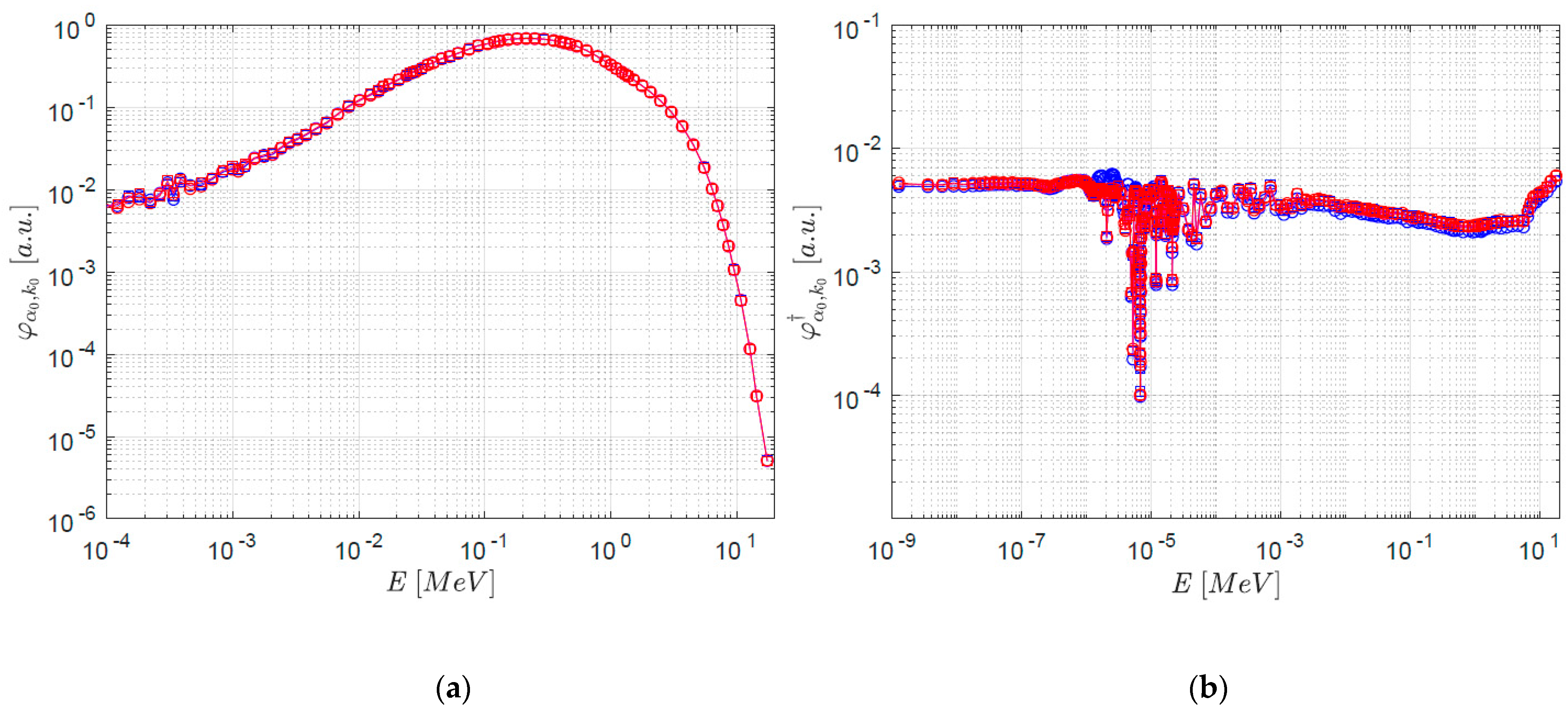
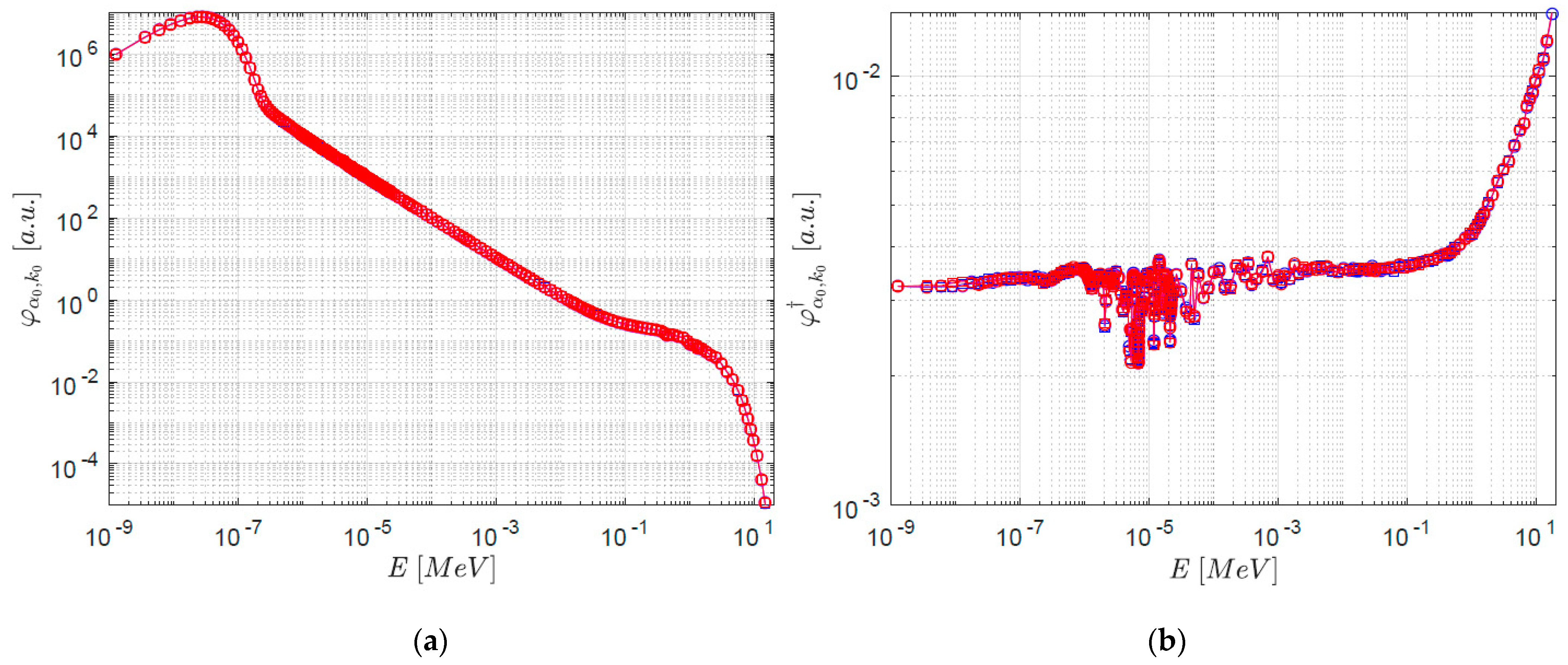
For illustration, the shapes of direct and adjoint eigenmodes ${\phi }_{k_0}^{(†)}$ and ${\phi }_{{\alpha }_0}^{(†)}$ (with and without delayed neutron contributions) for the sub-critical configuration and the super-critical configuration of Problem I are shown in Figure 1 and Figure 2, respectively. For comparison, all curves have been normalized. Deviations due to the kind of eigenfunction (either k or α) and to the presence of delayed contributions are clearly visible in the adjoint distributions.

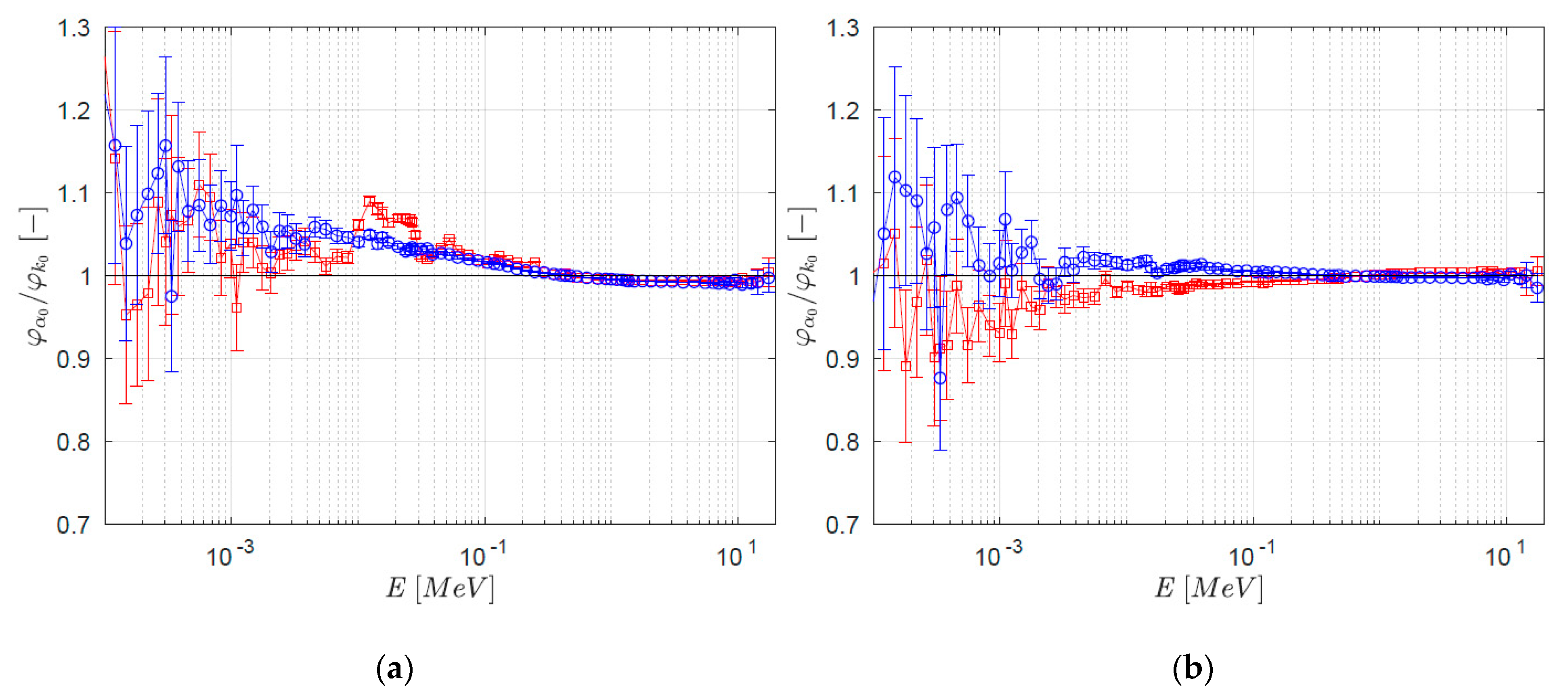
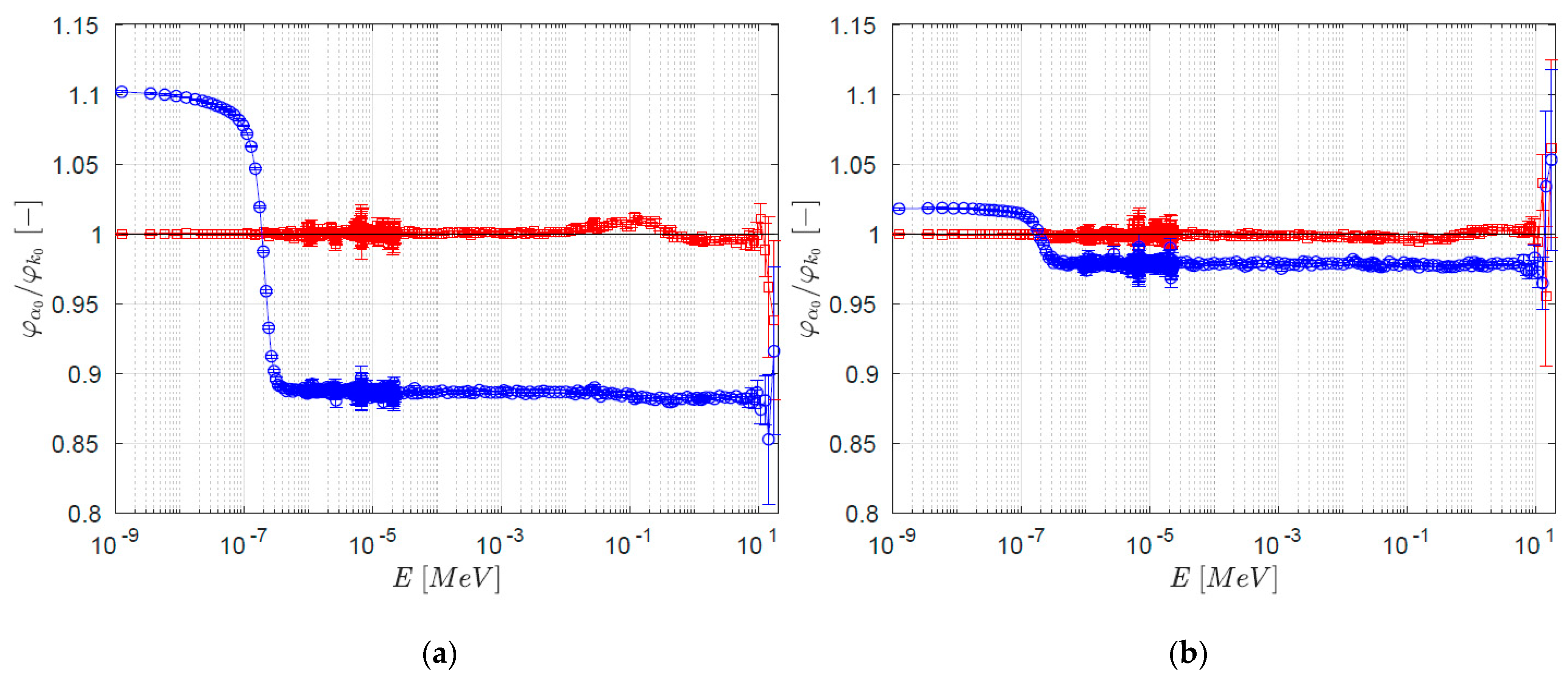
In order to quantitatively assess these differences, in Figure 3 and Figure 4 we show the ratios between α- and k- eigenfunctions for the direct and adjoint problem, respectively. For the direct eigenfunctions, deviations are overall rather small (see Figure 3). In the sub-critical configuration, we have ${\phi }_{{\alpha }_0}^{}$ < ${\phi }_{k_0}^{}$ in the fast region and vice-versa in the epithermal region, both with and without delayed neutrons (Figure 3a). For the super-critical configuration, the situation is different: in the fast region, we have ${\phi }_{{\alpha }_0}^{}$ < ${\phi }_{k_0}^{}$ without delayed neutrons and ${\phi }_{{\alpha }_0}^{}$ > ${\phi }_{k_0}^{}$ with delayed neutrons; in the epithermal region the behaviour is inverted. This is possibly due to the fact that in the super-critical configuration the sign of α₀ changes with or without delayed neutrons. In the thermal region, very few neutrons contribute to the direct eigenfunctions (as expected from a fast neutron spectrum system), although statistical uncertainty prevents from drawing solid conclusions.

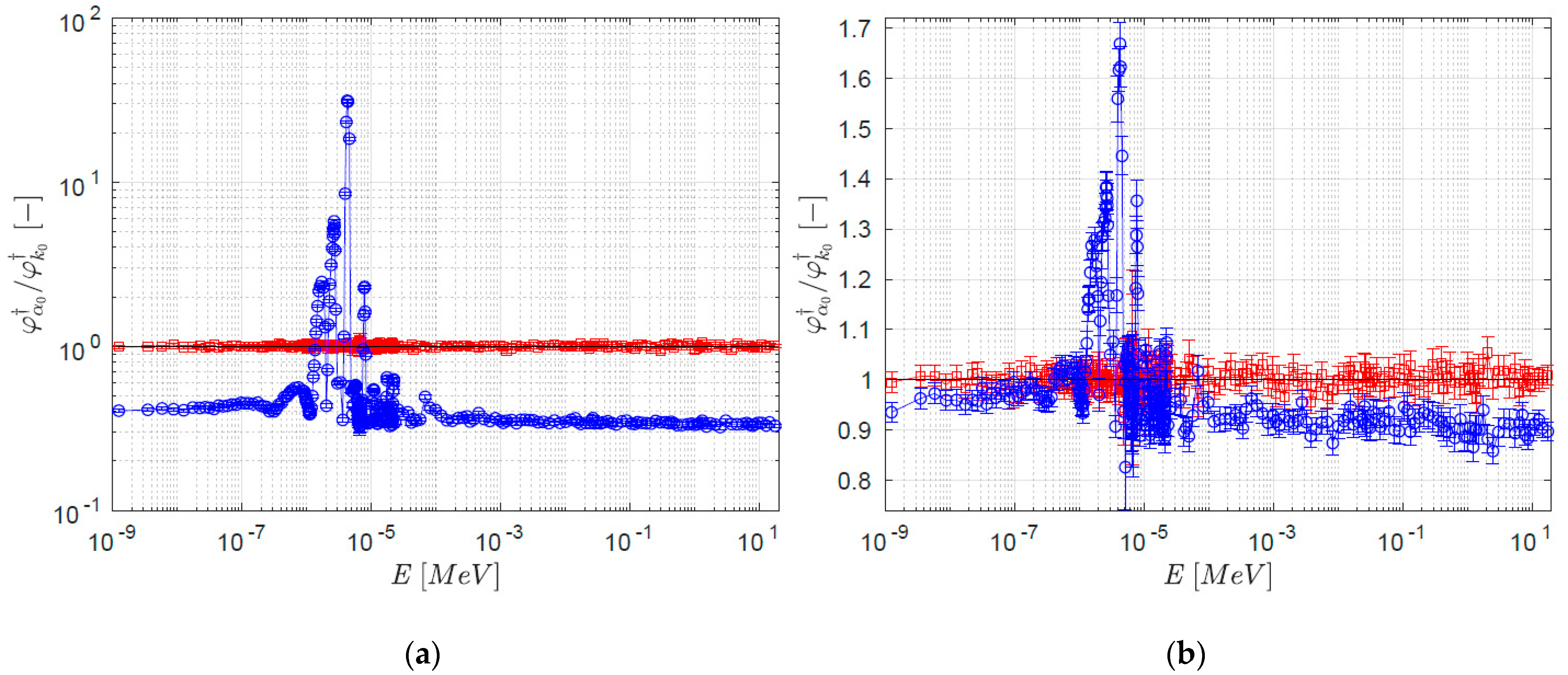
As for the adjoint eigenfunctions, deviations are somewhat stronger when delayed neutrons are not considered (see Figure 4), especially in the resonance region. On the contrary, when delayed neutron contributions are taken into account deviations of ${\phi }_{k_0}^{†}$ from ${\phi }_{{\alpha }_0}^{†}$ become much smaller. Overall, neglecting the presence of delayed neutrons leads to ${\phi }_{{\alpha }_0}^{†}$< ${\phi }_{k_0}^{†}$ outside the resonance region and the difference between the two distributions is larger for the more sub-critical configuration.

Direct and adjoint eigenmodes computed by including delayed neutrons show similar distributions. In principle, the absolute value of α₀ drops around 10⁻¹ s⁻¹, therefore the term (α₀/υ)${\phi }_{{\alpha }_0}^{}$ is significantly reduced. Moreover, the weight multipliers for both the k-delayed fission operator (1/k₀) and the α-delayed fission operator ${\lambda }_j/({\lambda }_j+{\alpha }_0)$ are both around the unit value. For this reason, the k- and the α- eigenvalue problems presented in Equations (1) and (2) for the direct formulation and in Equations (4) and (5) for the adjoint formulation would be close to each other.

3.2.2. Problem III

The fundamental eigenvalues k₀ and α₀ computed in the corresponding simulations for Problem III with and without the delayed neutron contributions are given in

Table 6. Fundamental eigenvalues k₀ for Problem III.

Configuration	k0 [–], with Delayed Contributions	k0 [–], Prompt Fission Only
III sub-critical	0.9927 ± 2 × 10−4	0.9858 ± 2 × 10−4
III super-critical	1.0050 ± 2 × 10−4	0.9979 ± 2 × 10−4

and

Table 7. Fundamental eigenvalues α₀ for Problem III.

Configuration	α0 [s–1], Including Precursors	α0 [s–1], without Precursors
III sub-critical	−1.1686 × 10−2 ± 7 × 10−6	−9.820 × 102 ± 9 × 10−1
III super-critical	4.71 × 10−1 ± 1 × 10−3	−1.945 × 102 ± 4 × 10−1

, respectively. It is worth noting that similarly to Problem I the system described in Problem III is sub-critical if delayed neutron contributions are neglected in the calculations. Moreover, the fundamental eigenvalue k₀ is reduced by approximately 700 pcm when the delayed contributions are not considered. Concerning the α-eigenvalue formulation, the absolute value of α₀ is again smaller than 1 s⁻¹ by including delayed neutrons, whereas the absolute value of this eigenvalue is between 10² s⁻¹ and 10³ s⁻¹ when neglecting delayed neutrons. Neglecting the presence of the delayed neutrons in this thermal system implies a decrease of the reactor period of approximately 3 orders of magnitude.

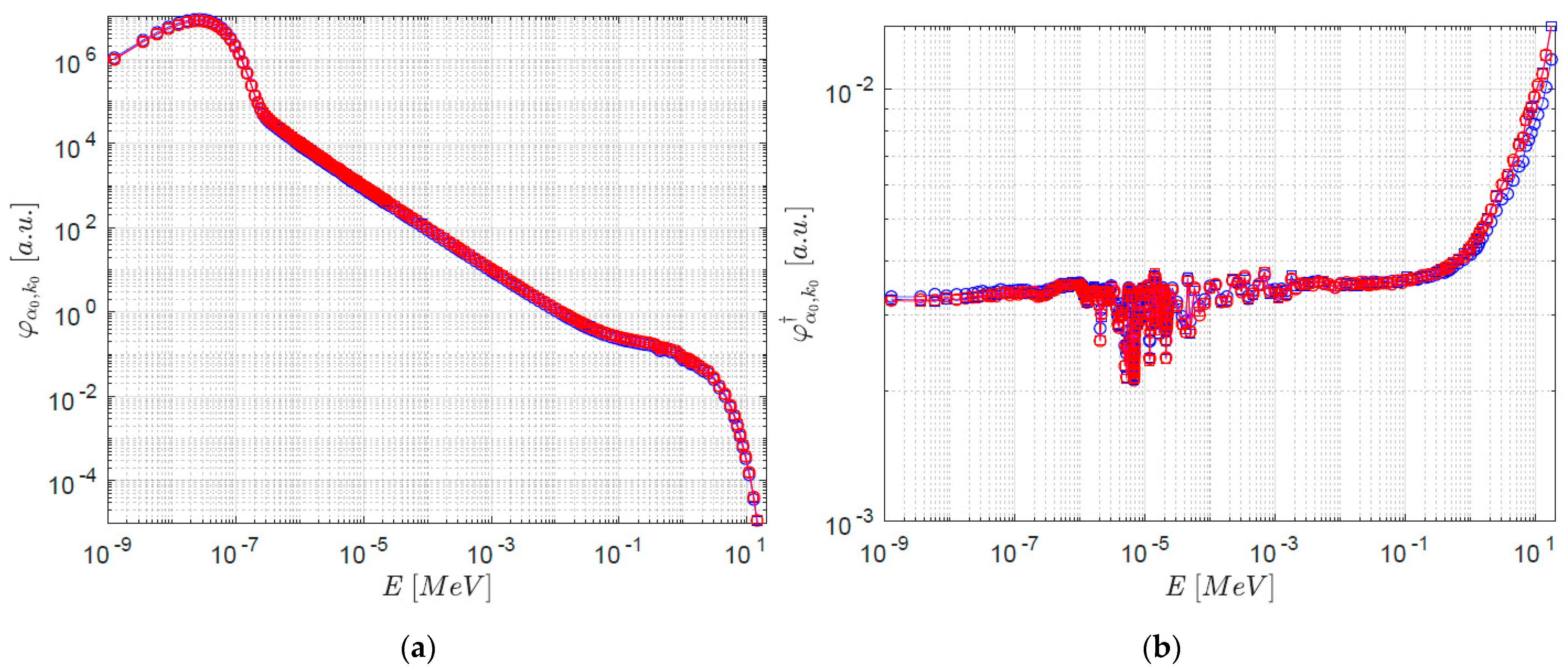
The shapes of the direct eigenmodes ${\phi }_{k_0}^{}$ and ${\phi }_{{\alpha }_0}^{}$ (with and without delayed neutron contributions) for the sub-critical configuration of Problem III are shown in Figure 5a; the adjoint eigenmodes are also shown in Figure 5b. The direct and the adjoint distributions for the super-critical configuration of the same problem are shown in Figure 6. The behaviour of the adjoint eigenmodes shows noticeable differences with respect to what observed in spatially large systems, i.e., MOX and UOX assembly configurations [19], where the thermal component was higher and the fast component was lower as compared to Problem III. The strong impact of the fast component in our example, and the milder impact of the thermal component, can be justified by the fact that Problem III is strongly spatially heterogeneous, with a fast spectrum localized in the fissile lump and a thermal spectrum localized in the moderator. Due to normalization the amplitude of ${\phi }_{}^{†}$ shown in Figure 5 and Figure 6 is smaller in the thermal region and larger in the fast region if compared to the results obtained from MOX and UOX assembly configurations. For comparison, all curves have been normalized. Slight but significant deviations due to the kind of eigenfunction (either k-or α-) and to the presence of delayed contributions are again visible, especially for the adjoint fluxes.

The corresponding ratios for the direct and adjoint eigenfunctions are displayed in Figure 7 and Figure 8, respectively. For the direct eigenfunctions, when delayed neutron contributions are taken into account deviations are rather small (see Figure 7) for both the sub- and super-critical configurations. However, it is possible to notice the presence of a deviation between the k- and α-eigenfunctions: for the sub-critical configuration, we have ${\phi }_{{\alpha }_0}^{}$ < ${\phi }_{k_0}^{}$ for energy values larger than 0.6 MeV and ${\phi }_{{\alpha }_0}^{}$ > ${\phi }_{k_0}^{}$ for energy values larger between 10 keV and 0.6 MeV; for the super-critical configuration an opposite behavior is noticeable in the same energy ranges. This inversion is justified by the transition from a sub-critical to a super-critical system. For a sub-critical configuration, the k-eigenvalue formulation hardens the energy spectrum by artificially increasing the amplitude of fission operator by a factor 1/k₀, whereas the α-eigenvalue formulation promotes the thermal spectrum by the term α₀/υ and at the same modifies the delayed fission operator by the factor γ = $\overline{\lambda }$/(α₀ + $\overline{\lambda }$). Observe that we have γ > 1 for negative α₀ and γ < 1 for positive α₀. The presence of delayed neutrons shifts the behaviour where ${\phi }_{{\alpha }_0}^{}$ < ${\phi }_{k_0}^{}$ towards 0.6 MeV which is around the average emission energy for delayed neutrons [22]. According to the α-eigenvalue formulation, the delayed fission operator is now rescaled by a factor $\overline{\lambda }$/($\overline{\lambda }$ + α₀), with $\overline{\lambda }$ = β/∑_j(β_j/λ_j) = 0.0768 ± 0.0006 s⁻¹ for U²³⁵ [23]. This factor is still smaller than 1/k₀, hence ${\phi }_{{\alpha }_0}^{}$ is still smaller than ${\phi }_{k_0}^{}$ at fast energy range. The symmetric argument can be applied for the super-critical case.

The ratio shown for energies between 10 keV and 20 MeV for the super-critical configuration seems smaller compared to the one computed for the sub-critical configuration. This result is coherent with the former configuration being closer to the critical state (super critical configuration) with respect to the latter (sub-critical configuration). For energy ranges smaller than 10 keV, no significant differences are visible.

On the contrary, for the simulations excluding delayed neutrons deviations become larger: in the fast and epithermal region, we have ${\phi }_{{\alpha }_0}^{}$ < ${\phi }_{k_0}^{}$, whereas ${\phi }_{{\alpha }_0}^{}$ > ${\phi }_{k_0}^{}$ in the thermal region. Again, if only prompt neutrons are considered, the fundamental eigenmode ${\phi }_{k_0}^{}$ is shifted towards higher energies for a sub-critical system due to the 1/k₀ factor which artificially increases the number of fissions. This behaviour is smoothed in the supercritical configuration (which is sub-critical, if delayed contributions are neglected) due to the system being closer to the critical state. As for the adjoint eigenfunctions, strong deviations in the fast region (E > 0.1 MeV) are observed for the sub-critical configuration, when delayed neutrons are not considered (see Figure 8). In all the other configurations, no significant differences are visible.

3.3. Analysis of the Effective Kinetics Parameters

Based on the observed discrepancies between the fundamental k- and α-eigenmodes, it would be interesting to assess which is the practical impact on the reactor parameters that depend on these quantities. In this respect, a prominent example is represented by the kinetics parameters, which are indeed bilinear forms depending on both the forward and the adjoint eigenmodes. The expressions of the effective mean generation time Λ_eff(α,k) and the effective delayed fraction ${\beta }_{\mathrm{eff}(\alpha ,k)}^j$ respectively read

$${\beta }_{\mathrm{eff}(\alpha ,k)}^j=\frac{<{\phi }_{(\alpha ,k)}^{†},\frac{x_d^j}{4\pi }{F}_d^j{\phi }_{(\alpha ,k)}>}{<{\phi }_{(\alpha ,k)}^{†},F{\phi }_{(\alpha ,k)}>},$$

(6)

$${\Lambda }_{\mathrm{eff}(\alpha ,k)}^{}=\frac{<{\phi }_{(\alpha ,k)}^{†},\frac{1}{\upsilon }{\phi }_{(\alpha ,k)}>}{<{\phi }_{(\alpha ,k)}^{†},F{\phi }_{(\alpha ,k)}>}.$$

(7)

The kinetics parameters, in turn, influence the system reactivity, through the in-hour (Nordheim) formula [11,24]. The static reactivity ρ_k and the dynamic reactivity ρ_α follow from [11,12,13,24,25]

$${\rho }_k^{}=\frac{k_0-1}{k_0},$$

(8)

and

$${\rho }_{\alpha }^{}={\alpha }_0{\mathsf{\Lambda }}_{eff,\alpha }+{\displaystyle \sum _j\frac{{\alpha }_0{\beta }_{\mathrm{eff},\alpha }^j}{{\alpha }_0+{\lambda }_j}}.$$

(9)

The static reactivity ρ_k depends only be the fundamental eigenvalue k₀, whereas the dynamic reactivity ρ_α requires the computation of ${\mathsf{\Lambda }}_{eff,\alpha }$ and ${\beta }_{eff,\alpha }^j{}_{}$ in addition to the fundamental eigenvalue α₀. The IFP method and the G-IFP method allow the computation of the bilinear forms of the kind $<{\phi }_k^{†},A{\phi }_k^{}>$ and $<{\phi }_{\alpha }^{†},A{\phi }_{\alpha }^{}>$ respectively, given a generic operator A. Both k and α weighted effective kinetics parameters have been estimated by resorting the methods implemented in the development version of TRIPOLI-4^® [7].

The effective kinetics parameters estimated for Problem I are shown in

Table 8. Effective kinetics parameters of Problem I, sub-critical configuration including delayed contributions.

Parameters	$<{\mathit{\phi }}_{\mathit{\alpha }}^{†},•>$	$<{\mathit{\phi }}_{\mathit{k}}^{†},•>$
ρ [pcm]	−669 ± 5	−608 ± 6
Λeff [ns]	5.773 ± 0.003	5.728 ± 0.002
βeff [pcm]	644 ± 2	645 ± 2
${\beta }_{\mathrm{eff}}^1{}_{}$ [pcm]	23.5 ± 0.1	23.5 ± 0.4
${\beta }_{\mathrm{eff}}^2{}_{}$ [pcm]	90 ± 0.6	90.9 ± 0.8
${\beta }_{\mathrm{eff}}^3{}_{}$ [pcm]	66.8 ± 2	66.4 ± 0.7
${\beta }_{\mathrm{eff}}^4{}_{}$ [pcm]	128.7 ± 0.9	128 ± 1
${\beta }_{\mathrm{eff}}^5{}_{}$ [pcm]	198 ± 1	200 ± 1
${\beta }_{\mathrm{eff}}^6{}_{}$ [pcm]	63.2 ± 0.7	63.1 ± 0.7
${\beta }_{\mathrm{eff}}^7{}_{}$ [pcm]	58 ± 0.7	56.2 ± 0.6
${\beta }_{\mathrm{eff}}^8{}_{}$ [pcm]	15.9 ± 0.4	16.6 ± 0.3

and

Table 9. Effective kinetics parameters of Problem I, sub-critical configuration without delayed contributions.

Parameters	$<{\mathit{\phi }}_{\mathit{\alpha }}^{†},•>$	$<{\mathit{\phi }}_{\mathit{k}}^{†},•>$
ρ [pcm]	−6289 ± 50	−1266 ± 4
Λeff [ns]	45.6 ± 0.3	5.728 ± 0.002

for the sub-critical configuration. Values for β_eff weighted according to the k-formulation are statistically compatible to those weighted according to the α-formulation. Simulation parameters for the evaluation of these parameters are the same as those shown in Table 2, estimated by considering 20 latent generations. A slight difference is observed in the values of Λ_eff, whereas a relatively larger difference is observed between dynamic and static reactivity. The latter deviation may be justified by the fact that the dynamic reactivity ρ_α depends on the eigenfunction distributions integrated for the estimation of Λ_eff,α and β_eff,α (Equation (9)), whereas the static reactivity ρ_k only depends on the fundamental eigenvalue k₀. Significant differences are observed for both reactivity and effective mean generation time values when only prompt neutrons are considered. In this case, the difference on the adjoint eigenmodes from Figure 4a plays a significant role in weighting the kinetics parameters.

The results obtained from the super-critical configuration of the same problem are shown in

Table 10. Effective kinetics parameters of Problem I, super-critical configuration including delayed contributions.

Parameters	$<{\mathit{\phi }}_{\mathit{\alpha }}^{†},•>$	$<{\mathit{\phi }}_{\mathit{k}}^{†},•>$
ρ [pcm]	409 ± 9	388 ± 6
Λeff [ns]	5.654 ± 0.002	5.675 ± 0.002
βeff [pcm]	643 ± 5	644 ± 2
${\beta }_{\mathrm{eff}}^1{}_{}$ [pcm]	20 ± 2	23.8 ± 0.4
${\beta }_{\mathrm{eff}}^2{}_{}$ [pcm]	93 ± 3	91.1 ± 0.8
${\beta }_{\mathrm{eff}}^3{}_{}$ [pcm]	68 ± 2	65.5 ± 0.7
${\beta }_{\mathrm{eff}}^4{}_{}$ [pcm]	125 ± 2	128.3 ± 0.9
${\beta }_{\mathrm{eff}}^5{}_{}$ [pcm]	201 ± 2	200 ± 1
${\beta }_{\mathrm{eff}}^6{}_{}$ [pcm]	61.4 ± 0.8	60.9 ± 0.7
${\beta }_{\mathrm{eff}}^7{}_{}$ [pcm]	57.6 ± 0.7	57 ± 0.6
${\beta }_{\mathrm{eff}}^8{}_{}$ [pcm]	17.1 ± 0.4	16.9 ± 0.3

and

Table 11. Effective kinetics parameters of Problem I, super-critical configuration without delayed contributions.

Parameters	$<{\mathit{\phi }}_{\mathit{\alpha }}^{†},•>$	$<{\mathit{\phi }}_{\mathit{k}}^{†},•>$
ρ [pcm]	−247.2 ± 0.4	−261 ± 6
Λeff [ns]	5.698 ± 0.002	5.677 ± 0.002

. The system including delayed neutrons is super-critical and all kinetics parameters are statistically compatible. Conversely, a non negligible discrepancy is still noticeable between static and dynamic reactivities for the configuration without delayed contributions. Overall, minimal differences have been found between direct and adjoint eigenmodes according to the k- and the α-eigenvalue formulations, which is mirrored in the small discrepancies observed in the effective kinetic parameters.

For Problem III, the effective kinetics parameters computed for the sub-critical configuration are shown in

Table 12. Effective kinetics parameters of Problem III, sub-critical configuration including delayed contributions.

Parameters	$<{\mathit{\phi }}_{\mathit{\alpha }}^{†},•>$	$<{\mathit{\phi }}_{\mathit{k}}^{†},•>$
ρ [pcm]	−582 ± 10	−735 ± 20
Λeff [μs]	12.62 ± 0.05	12.71 ± 0.05
βeff [pcm]	704 ± 7	706 ± 7
${\beta }_{\mathrm{eff}}^1{}_{}$ [pcm]	25.4 ± 0.4	24 ± 1
${\beta }_{\mathrm{eff}}^2{}_{}$ [pcm]	97 ± 2	97 ± 2
${\beta }_{\mathrm{eff}}^3{}_{}$ [pcm]	74 ± 3	72 ± 2
${\beta }_{\mathrm{eff}}^4{}_{}$ [pcm]	134 ± 3	144 ± 3
${\beta }_{\mathrm{eff}}^5{}_{}$ [pcm]	223 ± 5	223 ± 4
${\beta }_{\mathrm{eff}}^6{}_{}$ [pcm]	70 ± 2	65 ± 2
${\beta }_{\mathrm{eff}}^7{}_{}$ [pcm]	63 ± 2	63 ± 2
${\beta }_{\mathrm{eff}}^8{}_{}$ [pcm]	19 ± 1	18 ± 1

and

Table 13. Effective kinetics parameters of Problem III, sub-critical configuration without delayed contributions.

Parameters	$<{\mathit{\phi }}_{\mathit{\alpha }}^{†},•>$	$<{\mathit{\phi }}_{\mathit{k}}^{†},•>$
ρ [pcm]	−1658 ± 7	−1437 ± 20
Λeff [μs]	16.88 ± 0.06	12.79 ± 0.05

. The results from the simulation including delayed contributions shows minimal discrepancies for the values of Λ_eff and β_eff, whereas a clear difference is found between ρ_k and ρ_α. Conversely, the differences in the eigenmode distributions from Figure 7and Figure 8 strongly influence the parameters obtained from the simulation without delayed neutrons.

The parameters describing the super-critical configuration of Problem III are shown in

Table 14. Effective kinetics parameters of Problem III, super-critical configuration including delayed contributions.

Parameters	$<{\mathit{\phi }}_{\mathit{\alpha }}^{†},•>$	$<{\mathit{\phi }}_{\mathit{k}}^{†},•>$
ρ [pcm]	478 ± 40	496 ± 20
Λeff [μs]	12.16 ± 0.04	12.21 ± 0.04
βeff [pcm]	681 ± 20	711 ± 7
${\beta }_{\mathrm{eff}}^1{}_{}$ [pcm]	22 ± 7	28 ± 1
${\beta }_{\mathrm{eff}}^2{}_{}$ [pcm]	97 ± 10	97 ± 2
${\beta }_{\mathrm{eff}}^3{}_{}$ [pcm]	77 ± 8	73 ± 2
${\beta }_{\mathrm{eff}}^4{}_{}$ [pcm]	132 ± 6	138 ± 3
${\beta }_{\mathrm{eff}}^5{}_{}$ [pcm]	215 ± 6	232 ± 4
${\beta }_{\mathrm{eff}}^6{}_{}$ [pcm]	65 ± 3	62 ± 2
${\beta }_{\mathrm{eff}}^7{}_{}$ [pcm]	61 ± 2	62 ± 2
${\beta }_{\mathrm{eff}}^8{}_{}$ [pcm]	18 ± 1	20 ± 1

and

Table 15. Effective kinetics parameters of Problem III, super-critical configuration without delayed contributions.

Parameters	$<{\mathit{\phi }}_{\mathit{\alpha }}^{†},•>$	$<{\mathit{\phi }}_{\mathit{k}}^{†},•>$
ρ [pcm]	−252 ± 1	−213 ± 20
Λeff [μs]	12.93 ± 0.05	12.29 ± 0.05

. The presence of delayed neutrons and the proximity to the critical state leads to statistically compatible values of the kinetics parameters. The results obtained from the simulation including only prompt neutrons show minimal differences for Λ_eff values, a slightly larger discrepancy is found between static and dynamic reactivity.

In conclusion, we have investigated the effective kinetics parameters related to the Godiva-like benchmark problems. As expected, the differences between k- and α- eigenmode distributions are mirrored in the discrepancies between the corresponding kinetics parameters. Overall, the reactivity ρ is more affected by the choice of the eigenvalue formulation than the other kinetics parameters Λ_eff and β_eff.

The kinetics parameters and the associated reactivities are crucial for the control and the safety of nuclear reactors. A comparison with existing measurements (which typically involve neutron noise detection combined with the application of a fitting procedure based on a formulation of the in-hour equation) might help in discriminating whether the k or a formulations have a prominent advantage over each other for the interpretation of these parameters.

4. Analysis of the Crocus Benchmark

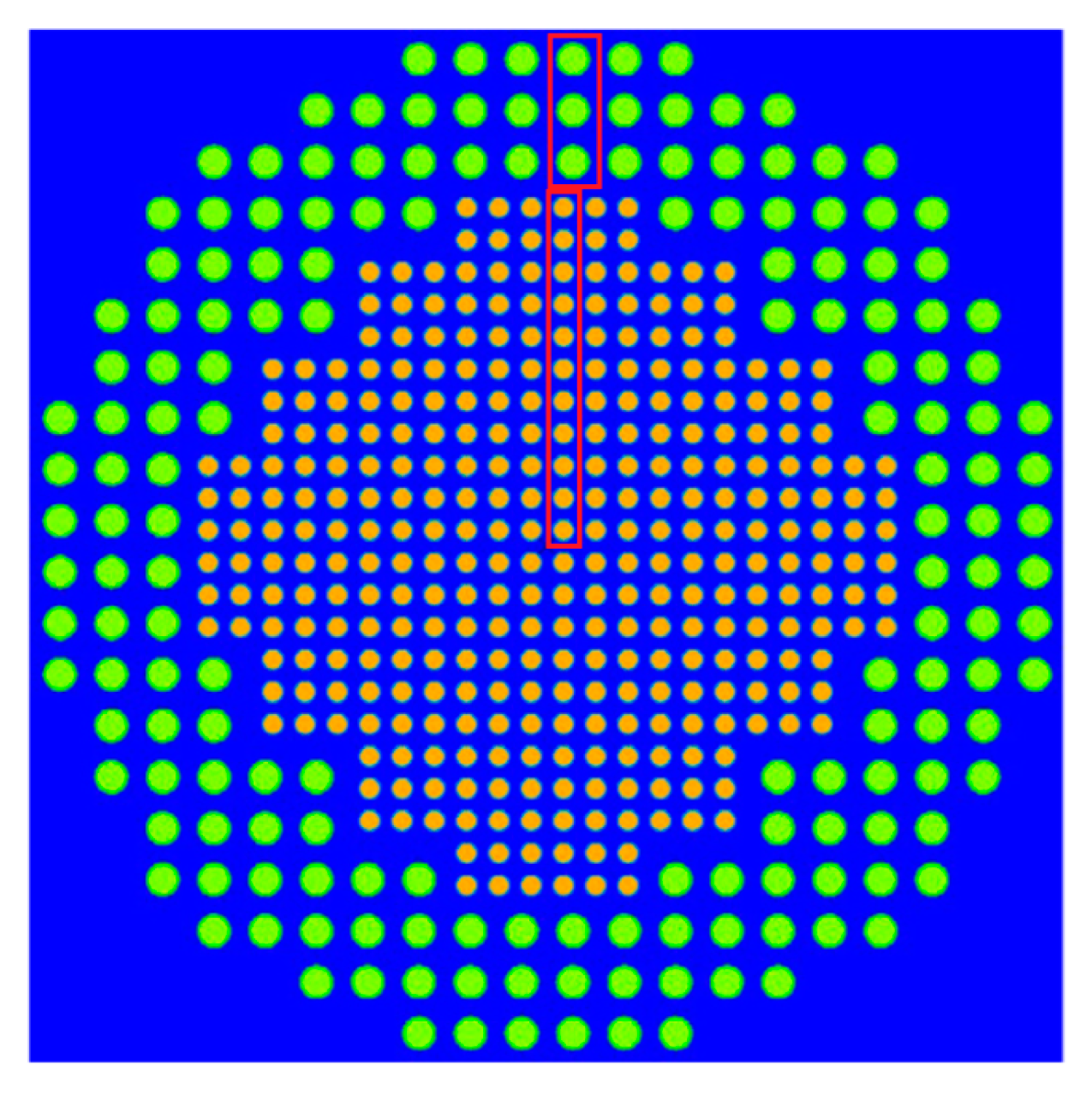
In order to take into account a more realistic configuration, and ascertain whether the conclusions reached in the previous section hold true for larger reactor cores, in this section we will consider two configurations of the CROCUS critical facility, operated at the Ecole Polytechnique Fédérale de Lausanne (EPFL), Switzerland. Thanks to its detailed description and careful measurements, the CROCUS core has been selected as an international benchmark for reactivity, kinetics parameters and reactor period calculations [14,15]. CROCUS is an open-tank type zero-power reactor, characterized by two fuel regions and moderated by light water. A radial section of this reactor is shown in Figure 9: the outer fuel rods (green) are composed of metallic uranium at 0.947 wt% ²³⁵U/U with 2.917 cm pitch, whereas the inner fuel rods (orange) are composed by UO₂ at 1.806 wt% ²³⁵U/U with 1.837 cm pitch. Details on the number and positions of these fuel rods are given in reference [15]. The core can be modeled as a cylinder with a diameter of about 60 cm and a height of 100 cm. The critical state of the system is controlled by the level of light water filling the reactor from the bottom cadmium plate. The critical configuration is achieved at a water level of 91.66 cm.

A preliminary comparison for this facility between fundamental α-eigenpairs and time dependent calculations has been carried out in [26]. Moreover, the kinetics parameters of the CROCUS core for the k-eigenvalue formulation has been previously computed in [4] and the associated reactivity was examined in [27]. In the following, we will investigate the behaviour of the fundamental forward and adjoint modes of the k and α formulations for this core, and we will then examine the impact of their respective shapes on the kinetics parameters and on the reactivity. For this purpose, we will consider two sub-critical configurations of the reactor, both obtained by lowering the water level. Configuration H1 is characterized by a water level equal to 90.8 cm, which induces a slightly sub-critical state. Configuration H2 is characterized by a water level equal to 80 cm, which corresponds to a more sub-critical condition. The fundamental eigenmodes will be computed by using TRIPOLI-4^® over 111 energy meshes and along 14 fuel pin positions, from the core center to the outer region, denoted by the red rectangular regions in Figure 9. The number of cycles and the particles per cycle simulated for these configurations are listed in

Table 16. Numerical simulation parameters for CROCUS configurations during forward simulations.

Configuration	Active Cycles	Inactive Cycles	Particles
H1	5 × 103	5 × 103	2 × 104
H2	5 × 103	5 × 103	2 × 104

for the forward simulations and in

Table 17. Numerical simulation parameters for CROCUS configurations during adjoint simulations.

Configuration	Particles	Latent Generations
H1	2 × 107	20
H2	2 × 107	20

for the adjoint simulations.

4.1. Analysis of the Fundamental Eigenmodes

The fundamental eigenvalues k₀ and α₀ computed in the corresponding simulations for H1 and H2 configurations of the CROCUS reactor (with and without precursor contributions) are given in

Table 18. Fundamental eigenvalues k₀ for H1 and H2 configurations of the CROCUS reactor.

Configuration	k0 [–], with Delayed Contributions	k0 [–], Prompt Fission Only
H1	0.9995 ± 1 × 10−4	0.9918 ± 1 × 10−4
H2	0.9919 ± 1 × 10−4	0.9839 ± 1 × 10−4

and

Table 19. Fundamental eigenvalues α₀ for H1 and H2 configurations of the CROCUS reactor.

Configuration	α0 [s–1], Including Precursors	α0 [s–1], without Precursors
H1	−5.97 × 10−3 ± 2 × 10−5	−1.711 × 102 ± 2 × 10−1
H2	−1.1994 × 10−2 ± 3 × 10−6	−3.336 × 102 ± 2 × 10−1

, respectively. As expected, the computed values show a slight sub-critical level for configuration H1 and a larger sub-critical state for configuration H2. According to the results obtained from the k-eigenvalue formulation, the criticality level of both configurations decreases by approximately 780 pcm when delayed neutrons are neglected. Concerning the α-eigenvalue formulation, the absolute value of α₀ is smaller than 1.2 × 10⁻² s⁻¹ by including delayed neutrons, whereas the absolute value of this eigenvalue is larger than 10² s⁻¹ for the simulation without precursor contributions.

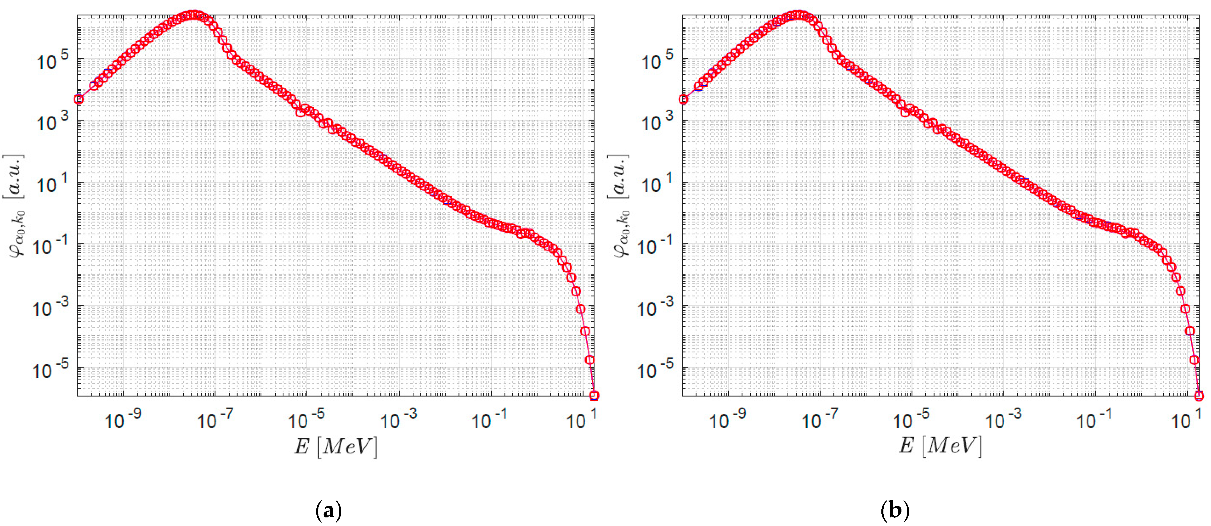
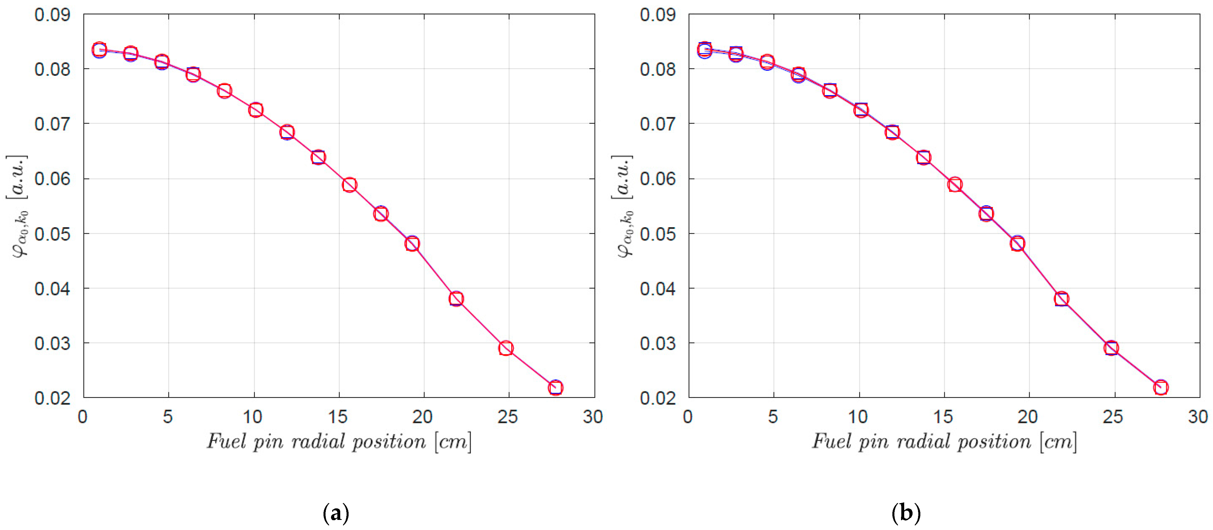
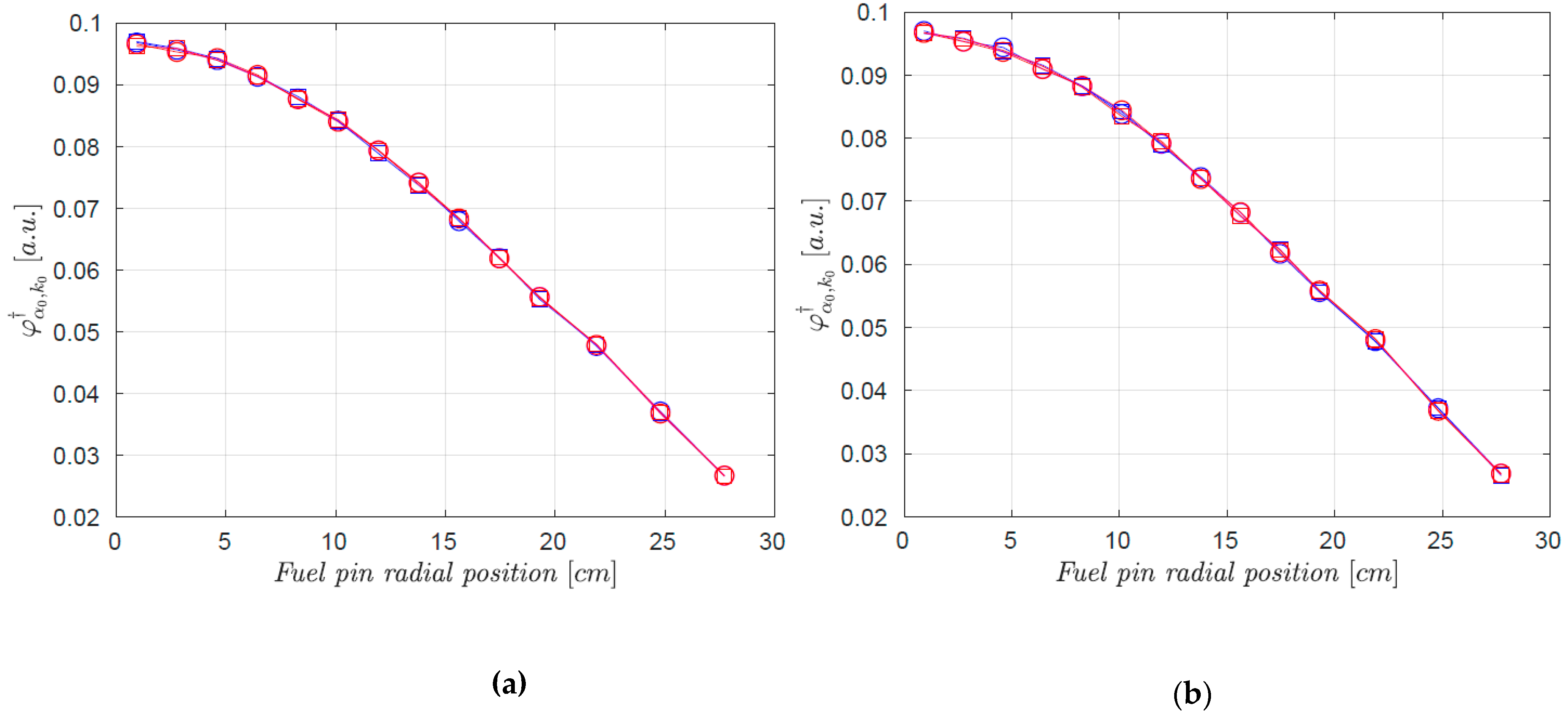
The shapes of direct eigenmodes ${\phi }_{k_0}^{}$ and ${\phi }_{{\alpha }_0}^{}$ (with and without delayed neutron contributions) are shown as a function of energy (Figure 10) and of the fuel pin position (Figure 11) for H1 (a) and H2 (b) configurations. The adjoint eigenmodes are shown as a function of the fuel pin position in Figure 12. All curves have been normalized. No major differences can be easily spotted in these figures, so that we have computed the ratios ${\phi }_{{\alpha }_0}^{}$/${\phi }_{k_0}^{}$ and ${\phi }_{{\alpha }_0}^{†}$/${\phi }_{k_0}^{†}$ in order to investigate possible discrepancies.

Figure 13 shows the ratios of the direct fundamental eigenmodes in the energy domain. The results obtained for configuration H1 (Figure 13a) are similar to those previously discussed for the Problem III of the benchmark configurations. When delayed neutrons are considered, no differences are visible between ${\phi }_{k_0}^{}$(E) and ${\phi }_{{\alpha }_0}^{}$(E). This is mainly due to the system reactivity being close to critical (about −50 pcm, as shown in Table 18): the k and α formulation are supposed to be very close to each other in this regime. If precursors are disregarded in the simulation, for this configuration the fundamental k-eigenmode is slightly different from the fundamental α-eigenmode: a shift towards high energy values is observed. The same behaviour is found for the H2 configuration (Figure 13b), characterized by a larger effect due to a larger sub-critical level with respect to the previous case (about −1600 pcm, as shown in Table 18). The effect of precursors is clearly visible for this configuration: the k-eigenmode displays significant discrepancies with respect to the α-eigenmode towards high energies for this sub-critical system, but ${\phi }_{{\alpha }_0}^{}$(E) > ${\phi }_{k_0}^{}$(E) only for E > 0.6 MeV, which is again similar to the findings of the Problem III configuration. Precursor contributions minimize the discrepancies between the two eigenvalue formulations and the delayed spectra move the threshold for ${\phi }_{{\alpha }_0}^{}$(E) > ${\phi }_{k_0}^{}$(E) at higher energy.

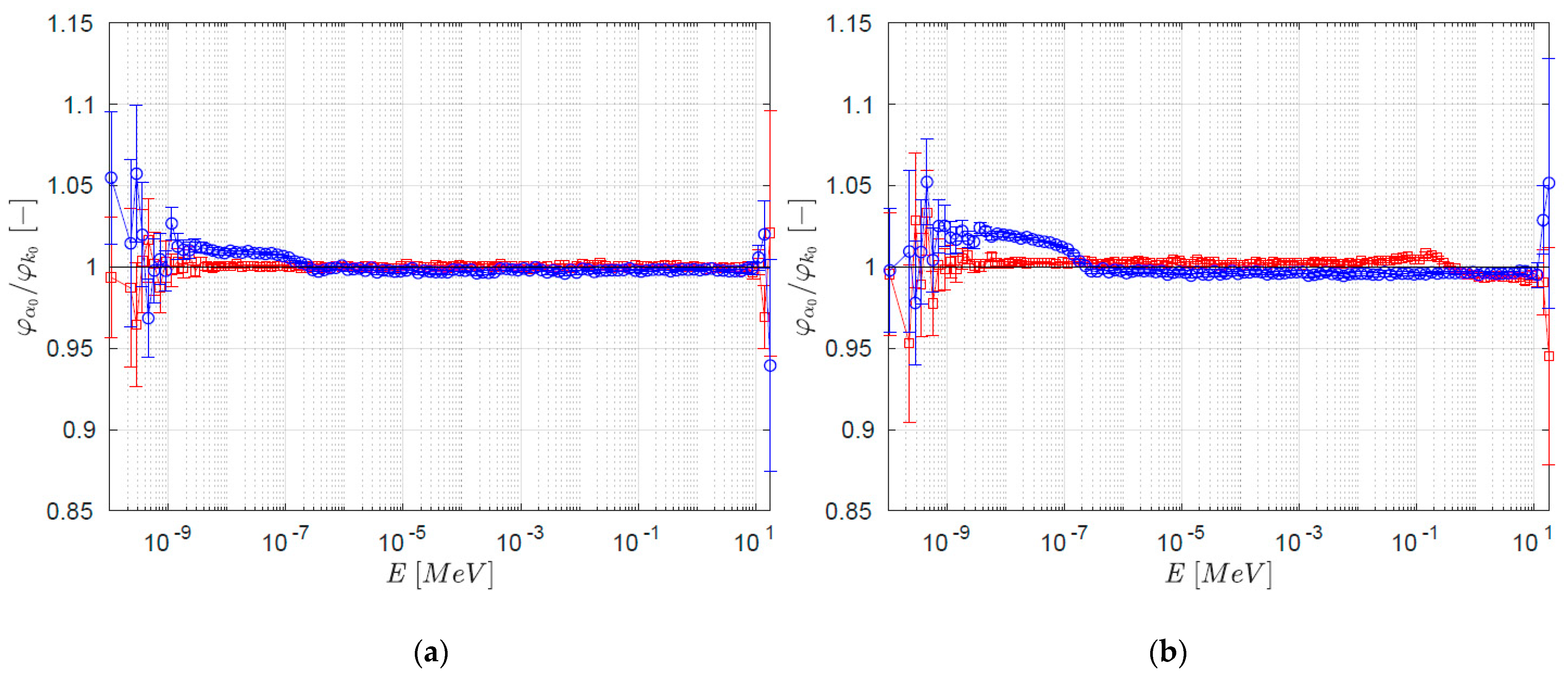
For the sake of completeness, we show the ratios of these eigenfunctions as a function of the fuel pin positions in Figure 14 for the direct formulation and in Figure 15 for the adjoint formulation. Overall, the behaviour of these two eigenmodes is similar: within uncertainty limits, no major differences can be detected with respect to the spatial coordinate.

4.2. Analysis of the Effective Kinetics Parameters

The effective kinetics parameters have been computed for the two CROCUS configurations by using the IFP and G-IFP of TRIPOLI-4^®.

Table 20. Effective kinetics parameters for the H1 configuration including delayed contributions.

Parameters	$<{\mathit{\phi }}_{\mathit{\alpha }}^{†},•>$	$<{\mathit{\phi }}_{\mathit{k}}^{†},•>$
ρ [pcm]	−73 ± 2	−50 ± 10
Λeff [μs]	47.69 ± 0.03	47.69 ± 0.03
βeff [pcm]	762 ± 4	760 ± 5
${\beta }_{\mathrm{eff}}^1{}_{}$ [pcm]	22.3 ± 0.6	23.4 ± 0.8
${\beta }_{\mathrm{eff}}^2{}_{}$ [pcm]	109 ± 2	113 ± 2
${\beta }_{\mathrm{eff}}^3{}_{}$ [pcm]	66 ± 1	62 ± 1
${\beta }_{\mathrm{eff}}^4{}_{}$ [pcm]	141 ± 2	141 ± 2
${\beta }_{\mathrm{eff}}^5{}_{}$ [pcm]	249 ± 3	245 ± 3
${\beta }_{\mathrm{eff}}^6{}_{}$ [pcm]	81 ± 2	83 ± 2
${\beta }_{\mathrm{eff}}^7{}_{}$ [pcm]	68 ± 1	67 ± 1
${\beta }_{\mathrm{eff}}^8{}_{}$ [pcm]	26.5 ± 0.8	26 ± 0.8

shows the parameters computed for the H1 configuration with precursor contributions: the results obtained for both eigenvalue formulations are statistically compatible. As expected, the proximity to the critical level of this configuration implies very close values of the k-weighted and α-weighted effective kinetics parameters. Similar results are found in

Table 21. Effective kinetics parameters for the H1 configuration without delayed contributions.

Parameters	$<{\mathit{\phi }}_{\mathit{\alpha }}^{†},•>$	$<{\mathit{\phi }}_{\mathit{k}}^{†},•>$
ρ [pcm]	−824 ± 1	−827± 10
Λeff [μs]	48.15 ± 0.03	48.11 ± 0.03

by neglecting precursor contributions.

The effective kinetics parameters of the H2 configuration with precursor contributions are shown in

Table 22. Effective kinetics parameters for the H2 configuration including delayed contributions.

Parameters	$<{\mathit{\phi }}_{\mathit{\alpha }}^{†},•>$	$<{\mathit{\phi }}_{\mathit{k}}^{†},•>$
ρ [pcm]	−723 ± 10	−822 ± 10
Λeff [μs]	48.06 ± 0.03	48.01 ± 0.03
βeff [pcm]	763 ± 5	766 ± 5
${\beta }_{\mathrm{eff}}^1{}_{}$ [pcm]	23.2 ± 0.2	22.2 ± 0.7
${\beta }_{\mathrm{eff}}^2{}_{}$ [pcm]	113 ± 2	113 ± 2
${\beta }_{\mathrm{eff}}^3{}_{}$ [pcm]	64 ± 1	66 ± 1
${\beta }_{\mathrm{eff}}^4{}_{}$ [pcm]	140 ± 2	143 ± 2
${\beta }_{\mathrm{eff}}^5{}_{}$ [pcm]	247 ± 3	251 ± 3
${\beta }_{\mathrm{eff}}^6{}_{}$ [pcm]	82 ± 2	82 ± 2
${\beta }_{\mathrm{eff}}^7{}_{}$ [pcm]	68 ± 2	66 ± 1
${\beta }_{\mathrm{eff}}^8{}_{}$ [pcm]	24.8 ± 0.9	24 ± 0.8

. A discrepancy is observed between the static and the dynamic reactivity, whereas the average values of all the other kinetics parameters are within one standard deviation for the two eigenvalue formulations.

Table 23. Effective kinetics parameters for the H2 configuration without delayed contributions.

Parameters	$<{\mathit{\phi }}_{\mathit{\alpha }}^{†},•>$	$<{\mathit{\phi }}_{\mathit{k}}^{†},•>$
ρ [pcm]	−1621 ± 2	−1638 ± 10
Λeff [μs]	48.59 ± 0.03	48.39 ± 0.03

shows the parameters obtained when neglecting precursor contributions: no significant discrepancies are observed in the computed values.

5. Conclusions

Inspired by the analysis originally proposed by D. E. Cullen [12], we have applied Monte Carlo methods for the estimation of k and α fundamental eigenmodes. We have extended the findings discussed in [12] in two directions, by addressing the evaluation of the fundamental adjoint eigenmodes and the influence of precursor contributions. Additional information regarding the discrepancies between the two eigenvalue formulations was found by assessing the effective kinetics parameters weighted by the k- or by the α-eigenmodes. We have focused our attention on the analysis of two Godiva-like benchmark configurations and the CROCUS reactor. In this way, we have explored thermal and fast spectra, homogeneous and heterogeneous media, simplified and realistic systems.

Significant, albeit globally small, differences have been detected, as expected on physical grounds based on previous investigations. In particular, we have recovered the same behaviour previously analyzed [12] in the energy domain for the distribution of the direct fundamental eigenfunctions ${\phi }_{k_0}^{}$ and ${\phi }_{{\alpha }_0}^{}$, and we have found similar discrepancies in the corresponding adjoint fundamental distributions ${\phi }_{k_0}^{†}$ and ${\phi }_{{\alpha }_0}^{†}$. Moreover, the presence of precursors has a non-trivial influence on the eigenfunctions, and this impact has been carefully examined for each configuration. Overall, the presence of precursors reduces the discrepancies between the two eigenmodes.

As a general remark, based on the configurations investigated here, it seems that the discrepancies between the k- and α-eigenfunctions are enhanced by the presence of strong spatial heterogeneity, such as for a core surrounded by a thick moderator/reflector. In this case, the system will be characterized by multiple time scales (as shown in [12]), related to the different times required by the neutrons to explore the multiplying and the diffusing region. Then, it appears that the α-eigenvalue formulation is more sensitive to these different time scales than the k-eigenvalue formulation, which is coherent with α being related to the time behaviour of the system and k being related to the fission generation behavior. These discrepancies on the eigenmodes are mirrored in the kinetics parameters and on the reactivity. In this respect, it is interesting to remark that the CROCUS reactor can be basically considered as a homogeneous system, with minimal discrepancies between the α and k formulations.

An application related to the effective kinetics parameters is the estimation of the reactor period and the sub-criticality level of the system. Both quantities can also be measured during experiments by the pulsed neutron source method [1] and reactor noise analysis methods [2,4]. The choice of the optimal adjoint weighting function (${\phi }_{{\alpha }_{}}^{†}$ or ${\phi }_{k_{}}^{†}$) in order to compare the results computed from numerical simulations to those obtained from measurements depends on the procedure and the techniques adopted during the experiment. Moreover, mixing α and k weighted kinetics parameters can be considered for the estimation of α₀ and ρ [28].

References

- Pázsit, I.; Pál, L. Neutron Fluctuations: A Treatise on the Physics of Branching Processes; Elsevier: Oxford, UK, 2008. [Google Scholar]
- Nauchi, Y. Attempt to estimate reactor period by natural mode eigenvalue calculation. In Proceedings of the Joint International Conference on Supercomputing in Nuclear Applications + Monte Carlo (SNA + MC 2013), Paris, France, 27–31 October 2013. [Google Scholar]
- Zoia, A.; Brun, E. Reactor physics analysis of the SPERT III E-core with TRIPOLI-4®. Ann. Nucl. Energy 2016, 90, 71–82. [Google Scholar] [CrossRef] [Green Version]
- Zoia, A.; Nauchi, Y.; Brun, E.; Jouanne, C. Monte Carlo analysis of the CROCUS benchmark on kinetics parameters calculation. Ann. Nucl. Energy 2016, 96, 377–388. [Google Scholar] [CrossRef]
- Nauchi, Y.; Kameyama, T. Development of Calculation Technique for Iterated Fission Probability and Reactor Kinetic Parameters Using Continuous-Energy Monte Carlo Method. J. Nucl. Sci. Technol. 2010, 47, 977–990. [Google Scholar] [CrossRef]
- Kiedrowski, B.C.; Brown, F.B.; Wilson, P.P.H. Adjoint-Weighted Tallies for k-Eigenvalue Calculations with Continuous-Energy Monte Carlo. Nucl. Sci. Eng. 2011, 168, 226–241. [Google Scholar] [CrossRef]
- Truchet, G.; Leconte, P.; Santamarina, A.; Brun, E.; Damian, F.; Zoia, A. Computing adjoint-weighted kinetics parameters in TRIPOLI-4®. Ann. Nucl. Energy 2015, 85, 17–26. [Google Scholar] [CrossRef] [Green Version]
- Terranova, N.; Mancusi, D.; Zoia, A. New perturbation and sensitivity capabilities in TRIPOLI-4®. Ann. Nucl. Energy 2018, 121, 335–349. [Google Scholar] [CrossRef]
- Endo, T.; Yamamoto, A. Sensitivity analysis of prompt neutron decay constant using perturbation theory. J. Nucl. Sci. Technol. 2018, 55, 1245–1254. [Google Scholar] [CrossRef]
- Jinaphanh, A.; Zoia, A. Perturbation and sensitivity calculations for time eigenvalues using the Generalized Iterated Fission Probability. Ann. Nucl. Energy 2019, 133, 678–687. [Google Scholar] [CrossRef]
- Bell, G.; Glasstone, S. Nuclear Reactor Theory; Van Nordstrand Reinhold Company: New York, NY, USA, 1970. [Google Scholar]
- Cullen, D.E. Static and Dynamic Criticality: Are They Different? Technical Report UCRL-TR-201506; University of California Radiation Laboratory: Berkeley, CA, USA, 2003. [Google Scholar]
- Terranova, N.; Zoia, A. Generalized Iterated Fission Probability for Monte Carlo eigenvalue calculations. Ann. Nucl. Energy 2017, 108, 57–66. [Google Scholar] [CrossRef] [Green Version]
- OECD/NEA. Benchmark on the Kinetics Parameters of the CROCUS Reactor; Technical Report Plutonium Recycling; NEA: Singapore, Singapore, 2007. [Google Scholar]
- Paratte, J.M.; Früh, R.; Kasemeyer, U.; Kalugin, M.A.; Timm, W.; Chawla, R. A benchmark on the calculation of kinetic parameters based on reactivity effect experiments in the CROCUS reactor. Ann. Nucl. Energy 2006, 33, 739–748. [Google Scholar] [CrossRef]
- Brun, E.; Damian, F.; Diop, C.M.; Dumonteil, E.; Hugot, F.X.; Jouanne, C.; Zoia, A. TRIPOLI-4®, CEA, EDF and AREVA reference Monte Carlo code. Ann. Nucl. Energy 2014, 151–160. [Google Scholar] [CrossRef]
- Zoia, A.; Brun, E.; Damian, F.; Malvagi, F. Monte Carlo methods for reactor period calculations. Ann. Nucl. Energy 2015, 75, 627–634. [Google Scholar] [CrossRef]
- Brockway, D.; Soran, P.; Whalen, P. Monte Carlo Alpha Calculations; Technical Report LA-UR-85-1224; Los Alamos National Laboratory: Los Alamos, NM, USA, 1985. [Google Scholar]
- Terranova, N.; Truchet, G.; Zmijarevic, I.; Zoia, A. Adjoint neutron flux calculations with TRIPOLI-4®: Verification and comparison to deterministic codes. Ann. Nucl. Energy 2018, 114, 136–148. [Google Scholar] [CrossRef] [Green Version]
- ICSBEP. International Handbook of Evaluated Criticality Safety Benchmark Experiments; NEA/NSC/DOC(95)/03; OECD NEA: Paris, France, 2018. [Google Scholar]
- Santamarina, A.; Bernard, D.; Blaise, P.; Coste, M.; Courcelle, A.; Huynh, T.D.; Jouanne, C.; Leconte, P.; Litaize, O.; Mengelle, S.; et al. The JEFF-3.1.1 Nuclear Data Library; Technical Report JEFF Report 22; OECD-NEA Data Bank: Paris, France, 2009. [Google Scholar]
- Cullen, D.E. A Simple Model of Delayed Neutron Emission; Technical Report UCRL-TR-204743; University of California, Lawrence Livermore National Laboratory: Livermore, CA, USA, 2004. [Google Scholar]
- McLane, V. Data Formats and Procedures for the Evaluated Nuclear Data File, ENDF-6; Brookhaven National Laboratory: Upton, NY, USA, 2001. [Google Scholar]
- Keepin, G.R. Physics of Nuclear Kinetics; Addison-Wesley: Reading, UK, 1965. [Google Scholar]
- Henry, A.F. The Application of Inhour Modes to the Description of Non-Separable Reactor Transients. Nucl. Sci. Eng. 1964, 20, 338–351. [Google Scholar] [CrossRef]
- Nauchi, Y.; Zoia, A.; Jinaphanh, A. Analysis of time-eigenvalue and eigenfunctions in the CROCUS benchmark. In Proceedings of the PHYSOR 2020, Cambridge, UK, 28 March–2 April 2020. [Google Scholar]
- Zoia, A.; Jouanne, C.; Siréta, P.; Leconte, P.; Braoudakis, J.; Wong, L. Analysis of dynamic reactivity by Monte Carlo methods: The impact of nuclear data. Ann. Nucl. Energy 2017, 110, 11–24. [Google Scholar] [CrossRef] [Green Version]
- Endo, T.; Yamamoto, A. Conversion from prompt neutron decay constant to subcriticality using point kinetics parameters based on α- and keff-eigenfunctions. In Proceedings of the ICNC 2019, Paris, France, 15–20 September 2019. [Google Scholar]
Figure 1.
Problem I, sub-critical configuration, direct (a) and adjoint (b) fundamental distributions according to the α-(blue) and k-(red) eigenvalue formulations, with (squares) and without (circles) delayed contributions.
Figure 2.
Figure 3.
Problem I, ratios / of the direct fundamental distributions, for sub-critical (a) and super-critical (b) configuration, with (red squares) and without (blue circles) delayed contributions.
Figure 4.
Problem I, ratios / of the adjoint fundamental distributions, for sub-critical (a) and super-critical (b) configuration, with (red squares) and without (blue circles) delayed contributions.
Figure 5.
Problem III, sub-critical configuration, direct (a) and adjoint (b) fundamental distributions according to the α- (blue) and k- (red) eigenvalue formulations, with (squares) and without (circles) delayed contributions.
Figure 6.
Problem III, super-critical configuration, direct (a) and adjoint (b) fundamental distributions according to the α- (blue) and k- (red) eigenvalue formulations, with (squares) and without (circles) delayed contributions.
Figure 7.
Problem III, ratios / of the direct fundamental distributions, for sub-critical (a) and super-critical (b) configuration, with (red squares) and without (blue circles) delayed contributions.
Figure 8.
Problem III, ratios / of the adjoint fundamental distributions, for sub-critical (a) and super-critical (b) configuration, with (red squares) and without (blue circles) delayed contributions.
Figure 9.
Radial section of the CROCUS reactor obtained with TRIPOLI-4®. The inner fuel rods (UO2, orange) and the outer fuel rods (metallic U, green) are moderated by light water (blue). The red regions denotes the 14 fuel rod positions defined for the flux distribution [15].
Figure 10.
Direct fundamental eigenmodes of the CROCUS reactor as a function of the energy, H1 (a) and H2 (b) configurations according to the α- (blue) and k- (red) eigenvalue formulations, with (squares) and without (circles) precursor contributions.
Figure 11.
Direct fundamental eigenmodes of the CROCUS reactor as a function of the fuel pin positions, H1 (a) and H2 (b) configurations according to the α- (blue) and k- (red) eigenvalue formulations, with (squares) and without (circles) precursor contributions.
Figure 12.
Adjoint fundamental eigenmodes of the CROCUS reactor as a function of the fuel pin positions, H1 (a) and H2 (b) configurations according to the α- (blue) and k- (red) eigenvalue formulations, with (squares) and without (circles) precursor contributions.
Figure 13.
Ratios / of the CROCUS reactor as a function of the energy variable, H1 (a) and H2 (b) configurations with (red squares) and without (blue circles) precursor contributions.
Figure 14.
Ratios / of the CROCUS reactor as a function of the fuel pin positions, H1 (a) and H2 (b) configurations with (red squares) and without (blue circles) precursor contributions.
Figure 15.