A Topology Optimization Procedure for Assisting the Design of Nuclear Components

Abstract

In this paper, we show that a module implemented in the MCNP transport code to perform sensitivity analyses can be diverted to perform topology optimizations of nuclear equipment. Component design with this approach leads to sophisticated solutions that outperform their human-designed counterparts.

1. Introduction

Suppose the operators of a silicon doping unit wish to design a neutron moderator that homogenizes the distribution of neutron capture sites in an irradiated ingot. Or suppose a medical physics team wishes to design a gamma-ray collimator, which has to be as efficient as possible in a limited volume. At present, these design studies are of a parametric nature. The characteristics of the aforementioned components are optimized using an intuitive subset of parameters, which includes the choice of materials to be used, as well as some geometrical parameters, e.g., the dimensions of subparts, the aperture angles, and so on. For each combination of these parameters, a simulation of the candidate device is performed, and the best solution emerging among them is chosen according to the objectives of the designers. This design practice is standard but it has a weak point. It relies on human intuition, which provides us with a general idea of the solution but generally lacks precision. To outmatch this human-based design, a transdisciplinary approach called topology optimization is blooming, alongside the increase in computing power [1]. This discipline aims at automatizing the design of equipment using algorithms able to take into account the physical laws involved while managing the objectives and constraints of the design. These algorithms already yield subtler, more performant solutions than human-based designs in a number of industrial fields [2,3,4,5]. In our field, however, there are still seldom applications of these techniques, presumably because of the large computing cost associated with an accurate solution of the Boltzmann equation. At the present times, the most advanced studies are focused on the development of radiation shields for spatial applications and on the fuel organization problem [6,7,8]. In these proceedings, relying on the theoretical framework proposed in [9], we will show that the PERT module implemented in the MCNP code [10,11,12] is precise and fast enough to perform realistic topology optimization of nuclear components. We will illustrate this progress with an application of practical interest, the design of a neutron spectrum shaper, and propose a benchmark on the optimization of the fuel distribution in a critical assembly.

2. Solving a Topology Optimization Problem with the MCNP Code

Consider a block of matter, whose mass density at a point r = (x, y, z) of space is denoted ρ(r). This block can be machined in various materials, whose respective atomic concentrations at the point r form a vector, denoted χ(r). A source, which can be external or intrinsic, fires particles into this block, whose transport can be modelled using a linear Boltzmann equation, B(ρ, χ)φ(r, E, Ω, ρ, χ) = Q(r, E, Ω), provided the density of particles remains low enough so that they do not interact with each other. In this equation, φ denotes the angular particle flux, function of the particle energies and directions, E and Ω, B is the Boltzmann operator, which depends on the physical characteristics ρ and χ of the block, and Q is the distribution in space, energies and directions of the source particles.

For industrial or scientific applications, one could search the best physical properties, (ρ_opt, χ_opt), of the aforementioned block of matter so that the particle population in a space region V optimizes a property desired by the operators of the particle source. For example, one could wonder how to machine a block of polyethylene so that the total flux of particles in V be as small as possible (design of a particle shield). To answer this kind of problem, one must solve an optimization problem, which can be written as

$$\begin{array}{ll}\underset{\rho ,\underset{¯}{\chi }}{\min /\max }& O\phi \left(\rho ,\underset{¯}{\chi }\right)\\ \mathrm{subject} \mathrm{to}& \begin{array}{l}\mathrm{B}\left(\rho ,\underset{¯}{\chi }\right)\phi \left(\underset{¯}{r},E,\underset{¯}{\Omega },\rho ,\underset{¯}{\chi }\right)=Q\left(\underset{¯}{r},E,\underset{¯}{\Omega }\right)\hfill \end{array}\\ \hfill & \underset{¯}{C}\left(\rho ,\underset{¯}{\chi },\phi \left(\rho ,\underset{¯}{\chi }\right)\right)=\underset{¯}{0}\hfill \end{array}$$

(1)

In Equation (1), O is a functional acting on the angular particle flux φ. The command min/max Oφ is the objective desired by the operators of the source; it could be, e.g., the minimization of the total particle flux at a point r_d for a radiation protection problem, in which case one would take min Oφ = ∫∫φ(r_d, E, Ω)dEdΩ. It could be the maximization of the radiation dose delivered in an area V of a body for a cancer treatment problem, in which case one would take max Oφ = ΔV⁻¹∫∫∫D(E)φ(r, E, Ω)drdEdΩ for r ∈ V, with D(E) being the flux-to-dose conversion function and ΔV the volume of area V. The optimization problem min/max Oφ is subject to some constraints, denoted C(ρ, χ, φ(ρ, χ)) = 0, the first one being the requirement that the particle transport obeys the Boltzmann equation, and the other ones being additional constraints, for example, a limitation over the maximum quantity of matter available (weight constraint), or a constraint over the k_eff of the system. This formalism is further discussed in Section 1 of [9].

To solve the optimization Problem (1), one can start from its Lagrangian formulation:

$$L\left(\rho ,\underset{¯}{\chi }\right)=O\phi \left(\rho ,\underset{¯}{\chi }\right)-\underset{¯}{\lambda }.\underset{¯}{C}\left(\rho ,\underset{¯}{\chi },\phi \left(\rho ,\underset{¯}{\chi }\right)\right)$$

(2)

where λ is a vector of Lagrange multipliers. The optimal properties of the particle propagator, (ρ_opt, χ_opt), which solve Problem (1), are then given by the following system of equations:

$$\begin{array}{ccc}{\left.\frac{\partial L}{\partial \rho }\right|}_{\rho ={\rho }_{opt},\underset{¯}{\chi }={\underset{¯}{\chi }}_{opt}}=0,& {\left.\frac{\partial L}{\partial \underset{¯}{\chi }}\right|}_{\rho ={\rho }_{opt},\underset{¯}{\chi }={\underset{¯}{\chi }}_{opt}}=\underset{¯}{0},& {\left.\frac{\partial L}{\partial \underset{¯}{\lambda }}\right|}_{\rho ={\rho }_{opt},\underset{¯}{\chi }={\underset{¯}{\chi }}_{opt}}=\underset{¯}{0}\end{array}$$

(3)

To solve this system, a solution is to segment the block into a large number N of small voxels, θ_{i = 1…N}. In each voxel θ_i, the density ρ(r) and fractions χ(r) are assumed constant, equal to ρ_i and χ_i. The derivatives (3) over functions ρ and χ thus become derivatives over parameters ρ_i and χ_i, whose computation can be performed with the PERT module implemented in the MCNP transport code [10]. Practical instructions on how to use the PERT module for computing derivatives are given in Section 1 of [9] for the computation of ∂L/∂ρ_i and in Section P of [9] (within the supplementary material file) for the computation of ∂L/∂χ_i. The PERT module relies on the differential operator sampling method, which is faster and more precise than the usual procedure based on the adjoint problem [1,7]. With this tool, all derivatives (3) can be computed in a single, direct MCNP calculation, which makes the precise resolution of a type (1) problem feasible in a humanly compatible time with the computer resources available in the 2020s. Equation (3) is then solved using an iterative algorithm, described in Section 2.2 of [9]. This algorithm starts from a uniform configuration, ρ_i = ρ₀ and χ_i = χ₀ ∀i, and then improves, iteration after iteration, the design of the structure by incrementing the parameters ρ_i and χ_i by small, discrete quantities, ±δρ and ±δχ, according to the constraints of Problem (1). This resolution procedure has been successfully tested over a large range of problems [9]. In these proceedings, we will illustrate its efficiency by solving two problems: the design of a neutron spectrum shaper in Section 3, and the minimization of a critical mass in Section 4.

3. Example of Application: Design of a Neutron Spectrum Shaper

Of all the possible applications of the optimization procedure described Section 2, the following problem stands out for two reasons: (i) it has a complex, non-linear objective functional O, whose handling is nonetheless possible with the approach described above; (ii) its formalism is transposable to a large category of problems, in fact all of those involving the calculation of a distance to an objective (see, e.g., the design of a gamma-ray collimator in Section 5.2 of [9]). This problem, therefore chosen to illustrate the methodology described in this paper, is stated below.

Problem. A 14 MeV neutron source is positioned at a point r_s, at a distance 100 cm from the center of a detection area (DA). The operators of the source have in stock 20 metric tons (~1.76 m³) of natural lead, and would like to shape it so that the energy spectrum $\varphi$(E) of neutrons in the detection area be as close as possible to an objective spectrum $\varphi$_obj(E). Find the design of such a neutron spectrum shaper.

First, let us tile space with N voxels θ_i, and denote ρ the vector of the lead mass densities ρ_{i = 1…N} in θ_i, and V the vector of the volumes V_i of these voxels. The detection area (here a cylinder of length 12.5 cm and radius 6.25 cm) is surrounded by a layer 1 cm thick of natural boron, whose mass density ρ_b is also to be optimized. With these notations, the design problem can be formulated as follows:

$$\begin{array}{l}\underset{\underset{¯}{\rho },{\rho }_b}{\min }d\left(\varphi ,{\varphi }_{obj}\right)=\frac{1}{2}-\frac{1}{2}\frac{{\displaystyle {\int }_E{\varphi }_{obj}\left(E\right)\varphi \left(E,\underset{¯}{\rho },{\rho }_b\right)w\left(E\right)dE}}{\sqrt{{\displaystyle {\int }_E{\varphi }_{obj}{\left(E\right)}^{2}w\left(E\right)dE}}\sqrt{{\displaystyle {\int }_E\varphi {\left(E,\underset{¯}{\rho },{\rho }_b\right)}^{2}w\left(E\right)dE}}}.\\ \mathrm{subject} \mathrm{to} P=\underset{¯}{\rho }.\underset{¯}{V}\le P_{\max }, {\rho }_{i=1\dots N}\le {\rho }_{\max }\end{array}$$

(4)

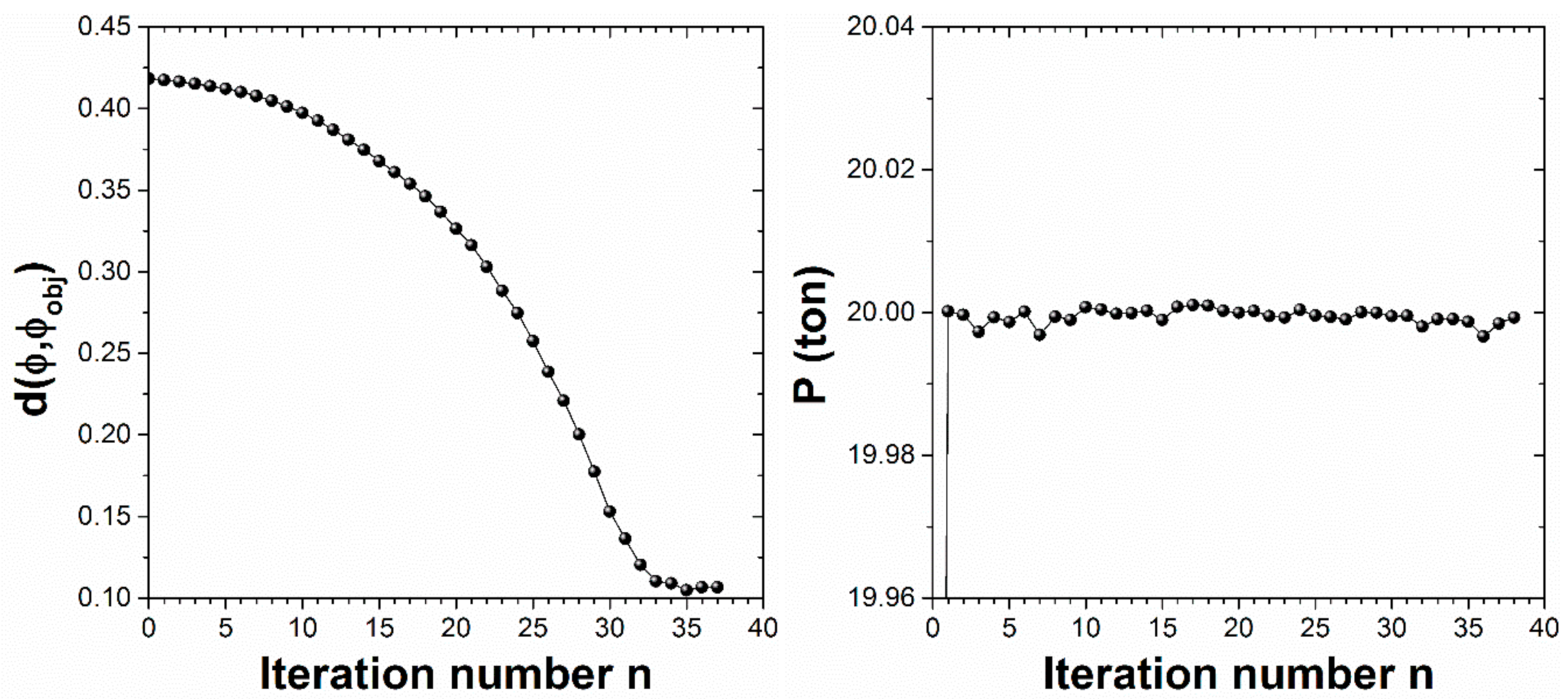
In Equation (4), P is the weight of the device, P_max the maximum permissible weight (20 tons here), ρ_max the natural mass density of lead (11.34 g/cm³), and d(ϕ, ϕ_obj) the distance between the energy spectrum ϕ(E) in the DA and the objective spectrum ϕ_obj(E), with w(E) being a weight function (here taken equal to 1/ϕ_obj²). The distance d is 0 iff ϕ(E) ∝ ϕ_obj(E), which is the objective of the design. In [9], the author attempted to solve this problem without the weight constraint, and with a small number of voxels. The result showed promises, but was not fully satisfactory as questions arose on the usefulness of the outer regions of the calculated structure. The weight constraint is introduced here to rationalize the positioning of the material in the device.

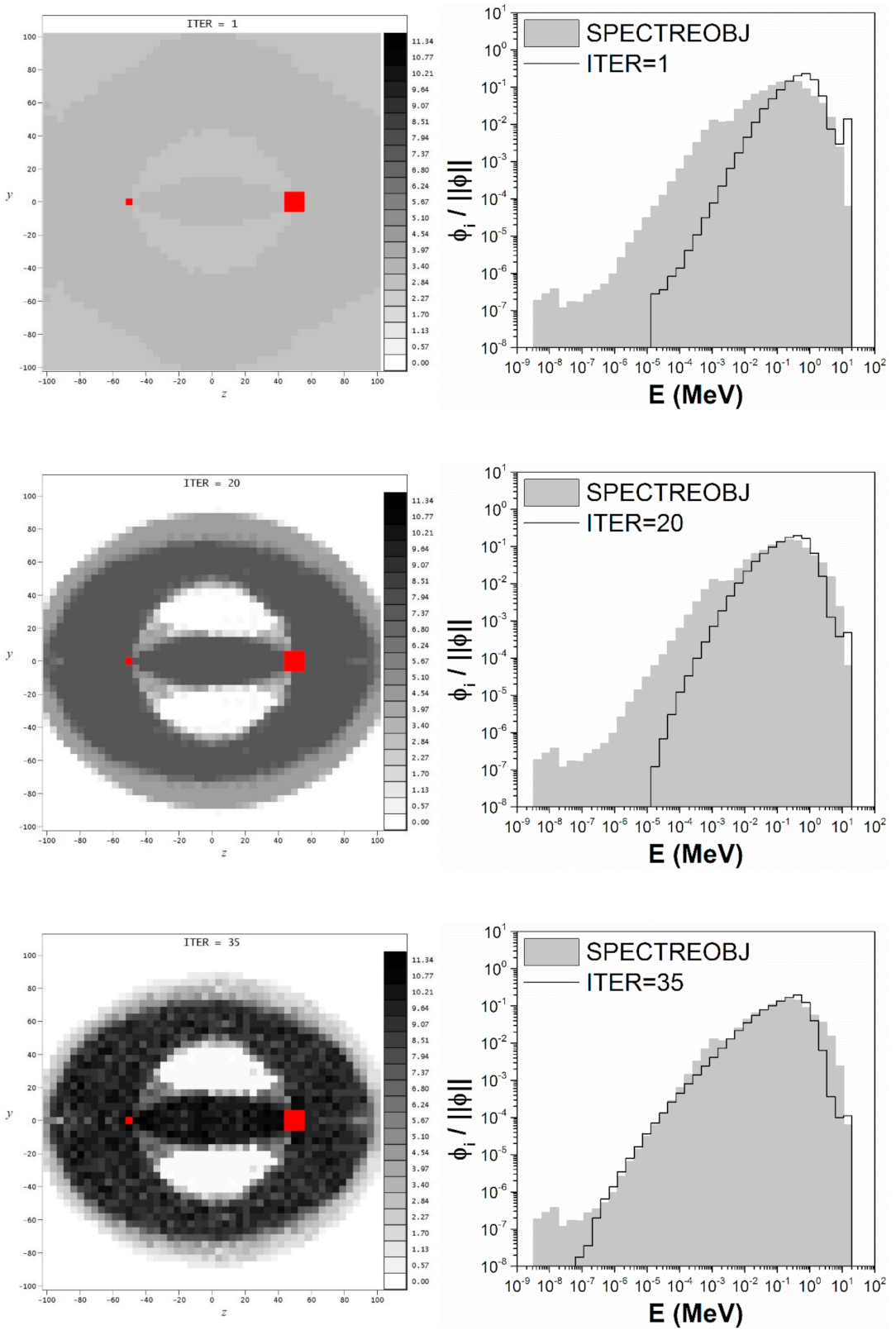
For this example, the chosen objective spectrum is typical of a fast reactor spectrum [13], and is displayed in gray on the right side of Figure 1. On the left side of Figure 1, the densities ρ in the voxels θ obtained with the optimization procedure are indicated for several iterations of the algorithm, using a gray scale whose unit is g/cm³. The units of the y and z axes are cm. The full 3D structure of the neutron spectrum shaper is generated by rotating these density maps around the symmetry axis y = 0. The small red cell on the left houses the 14 MeV source, and the larger red cell on the right is the DA. For each map, the normalized spectrum obtained in the detection area is given on the right.

The computations were performed using MCNP with cross-sections taken from JEFF-3.1. They lasted ~3 days/iteration on 24 CPU for 10⁹ source neutrons and 1145 cylindrical voxels. The evolutions of the distance d(ϕ, ϕ_obj) and of the weight P of the device with the iteration number n are given in Figure 2. As can be seen in Figure 1, the algorithm begins by accreting matter along the axis y = 0, which connects the source to the detection area, in order to slow down the 14 MeV neutrons. A reflector is simultaneously assembled around this central hub to increase the number of neutron collisions in the structure and shift the spectrum towards lower energies. The resulting device is efficient: the objective spectrum is correctly imitated over six orders of magnitude in energy, starting from n = 35. Differences still remain between the final spectrum at n = 35 and the objective spectrum, especially at high and low energy. These differences may be reduced by using a composite material, made of a mixture of lead and lighter isotopes, which will allow access to different neutron slowing-down modes.

4. Design Sensitivity to the Transport Data

The resolution of Problem (1) with a transport code naturally raises the question of the sensitivity of the computed design to the uncertainties on the transport data. More particularly, one may wonder if a slight modification of a transport datum, e.g., a change in the position or width of a cross-section resonance, could strongly alter the obtained optimal characteristics, (ρ_opt, χ_opt), of the device. In other words, could Problem (1) be subject to topological phase transitions? Despite its major interest, answering this question should prove difficult. Indeed, the resolution of the optimization problem is iterative, yet predicting the outcome of a complex iterative procedure is an open question in mathematics. To answer it, for a moment it will be necessary to be content with a Full Monte-Carlo approach. In this approach, a number of transport data sets could be sampled using the uncertainty data provided in the transport libraries; then, for each data set, Problem (1) could be solved. In the end, the uncertainty on the optimal design parameters (ρ_opt, χ_opt) could be evaluated by computing their average and variance. This approach is straightforward but, as the resolution of a type (1) problem typically requires times of the order of several CPU-months to several CPU-years depending on the number of voxels in the design, conducting it would require CPU-decades, which is a computing power the author did not have access to at the time of writing these proceedings.

In this section, a simple benchmark problem is hence proposed, which can make a good starting point for evaluating the uncertainties of the design arising from the uncertainties on the transport data, but also for comparing the designs obtained with transport codes other than MCNP and optimization approaches other than the one introduced in Section 2. This problem is stated below.

Problem. Consider a spherical assembly, 50 cm in radius, containing a mixture of low-enriched uranium (LEU, chemical formula: 97% at. ²³⁸U + 3% at. ²³⁵U) and polyethylene (PE, chemical formula CH₂). The assembly is made of 100 concentric spherical crowns θ_i, comprised between the radii R_i and R_{i + 1}, with R_i = 0.5i cm. Each crown θ_i contains a fraction χ_i of LEU and a complementary fraction (1 − χ_i) of PE. With these notations, the LEU mass M in the assembly is given by

$$M\left(\underset{¯}{\chi }=\left({\chi }_0,\dots ,{\chi }_{99}\right)\right)={\rho }_{LEU}\underset{¯}{\chi }.\underset{¯}{V}$$

(5)

where ρ_LEU = 19.0445 g/cm³ is the LEU mass density and V the vector of the volumes V_i of cells θ_i. The PE mass density is 0.94 g/cm³. Find the LEU fraction profile χ_opt that allows the assembly to achieve criticality with the smallest mass M of fuel possible.

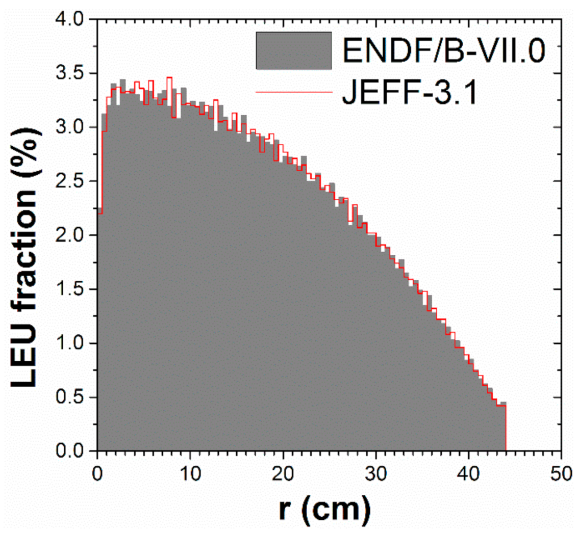
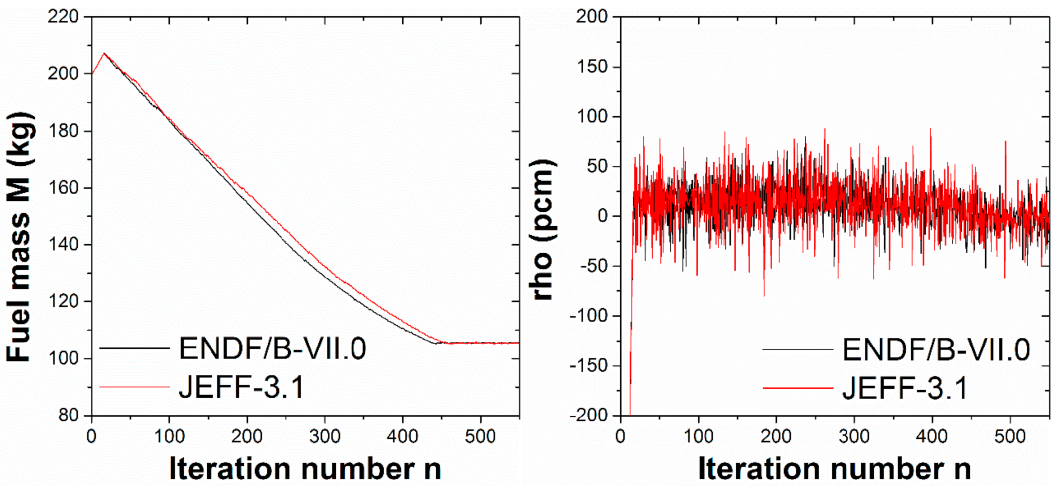
This problem can be solved using the approach described in Section 2. The full details of the procedure to follow are given in Section P of [9] (within the supplementary material file). The calculations were performed using MCNP with an iterative fission neutron distribution (KCODE mode, with 50 passive cycles and 100 active cycles of 2 × 10⁵ neutrons), with cross-sections taken from two libraries, ENDF/B-VII.0 and JEFF-3.1 (for both calculations, the thermal S(α, β) data in PE were taken from ENDF/B-VII.0). They lasted ∼20 min/iteration on 24 CPU. The LEU fraction profile that minimizes the critical mass is given in Figure 3, as a function of the distance r from the center of the assembly, for these two databases. The evolutions of the fuel mass M and of the reactivity rho = (k_eff − 1)/k_eff of the assembly, expressed in pcm unit, with the iteration number n of the optimization algorithm are given in Figure 4 for these two databases. The statistical errors on the reactivity values are ~9 pcm regardless of n.

In Figure 3, it is observed that the topology optimization algorithm generates a two-zone device: a fuel zone, comprised between r = 0 and 44 cm, surrounded by a reflector made of pure PE, for r > 44 cm. The fuel zone houses a small void at its center, from which the LEU fraction swiftly rises to reach a maximum of 3.4%, then decreases when r increases, to finally fall at 0 at r = 44 cm. The central void may however be a computation artefact. Indeed, it extends between r = 0 and 1 cm, in an area whose volume is only (1/50)³ = 8 × 10⁻⁴% of the full volume of the device, hence its negligible importance in the design, and the resulting large stat. errors on the k_eff perturbations in this area (see Figure 5). Overall, the LEU fractions are low everywhere. By thus diluting the fuel in the PE, the optimization algorithm generates a structure that efficiently thermalizes neutrons: 96% of the fissions in the device are due to thermal neutrons (E < 0.625 eV). The resulting structure is very efficient: 105.5 kg of 3% enriched uranium suffice to reach criticality. No significant differences are observed, whether in the design or the value of the minimum critical mass, between the results obtained with ENDF/B-VII.0 and JEFF-3.1 libraries, which constitutes a preliminary element of an answer on the robustness of the design.

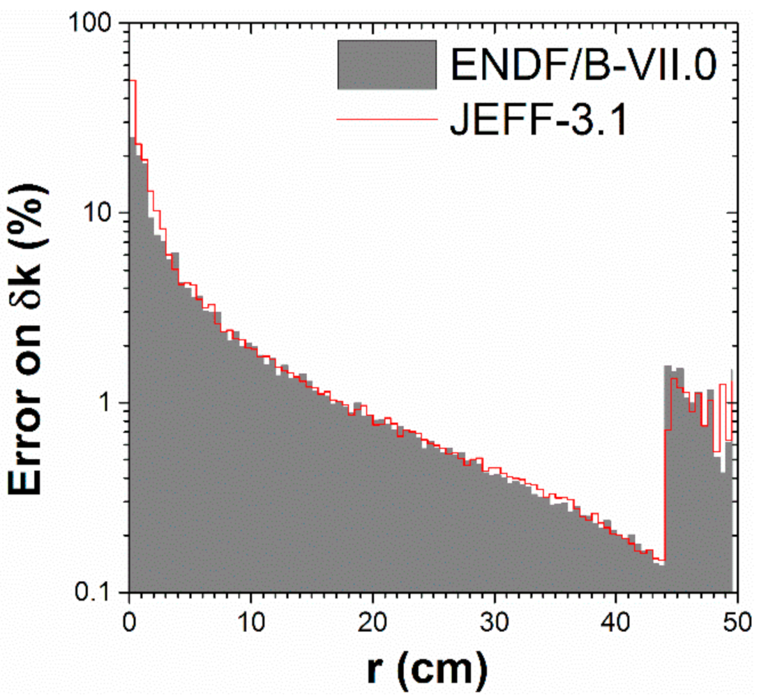
In Figure 3, one can observe the occurrence of small heterogeneities in the LEU fraction profiles, which are not mere statistical fluctuations. Indeed, the LEU fractions were purposely changed by very small increments, δχ = ±5 × 10⁻³%, between two iterations of the algorithm (hence the artificially large number of iterations to converge). This increment is small compared to the amplitude of the observed heterogeneities, ~0.2%. Hence, one might wonder if these heterogeneities play a role in reducing the critical mass. To investigate this question, the ENDF/B-VII.0 LEU fraction curve was smoothed using a Savitzky–Golay approach [14] while preserving the mass M. The reactivity obtained with the smoothed profile remained compatible with 0. The observed heterogeneities are therefore probably artifacts. The author sees three possible reasons for their occurrence: (1) a segregation induced by decorrelations of fission sites that may occur in a meter-size object; (2) a consequence of the non-zero stat. errors on the k_eff perturbations, δk_i = (∂k_eff/∂χ_i)δχ, computed with MCNP. Figure 5 illustrates the evolution with the distance r of this error, given in percent, computed for the optimal LEU profiles found with the ENDF/B-VII.0 and JEFF-3.1 libraries. However, complementary calculations involving higher numbers of source neutrons and KCODE active cycles were performed, yet showed similar heterogeneities, indicating that these two first leads are likely not the full answer; (3) a numerical issue induced by the printing format of the k_eff perturbations in MCNP outputs. Indeed, while all other perturbations computed by MCNP are printed in a scientific format, the k_eff ones stand out as being printed as integers in pcm unit. Therefore, when a k_eff perturbation is very small, lower than 1 pcm, yet non-null, it is actually printed 0 in MCNP output files, thus inducing a hidden numerical error. These technical considerations highlight the interest of benchmarking the results obtained in this section with other optimization approaches, e.g., with procedures that could use evolutionary algorithms or adjoint methods, as in [6,7,8].

5. Conclusions

In this paper, we showed that the PERT module implemented in the MCNP transport code, usually used to perform sensitivity analyses, can be diverted to automate the design of nuclear components. Two practical optimization problems were then solved using this tool, the design of a neutron spectrum shaper and the minimization of a critical mass, illustrating the potential of the proposed methodology.

References

- Bendsoe, M.P.; Sigmund, O. Topology Optimization: Theory, Methods and Applications; Springer: Berlin/Heidelberg, Germany, 2003. [Google Scholar]
- Takezawa, A.; Kobashi, M.; Kitamura, M. Porous composite with negative thermal expansion obtained by photopolymer additive manufacturing. APL Mater. 2015, 3, 076103. [Google Scholar] [CrossRef]
- Gaynor, A.T.; Meisel, N.A.; Williams, C.B.; Guest, J.K. Multiple-material topology optimization of compliant mechanisms created via PolyJet three-dimensional printing. J. Manuf. Sci. Eng. 2014, 136, 061015. [Google Scholar] [CrossRef] [Green Version]
- Zhu, J.H.; Zhang, W.H.; Xia, L. Topology optimization in aircraft and aerospace structures design. Arch. Comput. Method E 2016, 23, 595–622. [Google Scholar] [CrossRef]
- Andkjær, J.; Sigmund, O. Topology optimized low-contrast all-dielectric optical cloak. Appl. Phys. Lett. 2011, 98, 021112. [Google Scholar] [CrossRef] [Green Version]
- Asbury, S.; Holloway, J.P. Designing Shields for keV Photons with Genetic Algorithms. In Proceedings of the International Conference on Mathematics and Computational Methods Applied to Nuclear Science and Engineering 2011 (M&C 2011), Rio de Janeiro, Brazil, 8–12 May 2011. [Google Scholar]
- Pautz, S.D.; Adams, B.M.; Bruss, D.E. Geometric Uncertainty Quantification and Robust Design for 2D Satellite Shielding. In Proceedings of the International Conference on Mathematics and Computational Methods Applied to Nuclear Science and Engineering 2019 (M&C 2019), Portland, OR, USA, 25–29 August 2019. [Google Scholar]
- Allaire, G.; Castro, C. Optimization of nuclear fuel reloading by the homogenization method. Struct. Multidisc. Optim. 2002, 24, 11–22. [Google Scholar] [CrossRef]
- Chabod, S. Topology optimization in the framework of the linear Boltzmann equation–a method for designing optimal nuclear equipment and particle optics. Nucl. Instrum. Meth. A 2019, 931, 181–206. [Google Scholar] [CrossRef] [Green Version]
- Goorley, T.; James, M.; Booth, T.; Brown, F.; Bull, J.; Cox, L.J.; Durkee, J.; Elson, J.; Fensin, M.; Forster, R.A.; et al. Initial MCNP6 release overview. Nucl. Technol. 2012, 180, 298–315. [Google Scholar] [CrossRef]
- McKinney, G.W. A Monte-Carlo (MCNP) Sensitivity Code Development and Application. Master’s Thesis, University of Washington, Seattle, WA, USA, 1984. [Google Scholar]
- McKinney, G.W.; Iverson, J.L. Verification of the Monte Carlo Differential Operator Technique for MCNP; Los Alamos National Laboratory: Los Alamos, NM, USA, 1996. [Google Scholar]
- Laureau, A.; (CNRS, Université de Nantes, Nantes, France). Private Communication, 2017.
- Savitzky, A.; Golay, M.J. Smoothing and differentiation of data by simplified least squares procedures. Anal. Chem. 1964, 36, 1627–1639. [Google Scholar] [CrossRef]
Figure 1.
Iterative design of a neutron spectrum shaper with the optimization procedure.
Figure 2.
Evolutions of the distance d and of the weight P of the device with the iteration number n.
Figure 3.
Optimal low-enriched uranium (LEU) fraction profile as a function of the distance r from the assembly center.
Figure 4.
Evolutions of the fuel mass M and the reactivity rho in pcm with the iteration number n.
Figure 5.
Evolution with r of the stat. relative errors on the keff perturbation values at n = 500.
Publisher’s Note: MDPI stays neutral with regard to jurisdictional claims in published maps and institutional affiliations. |
© 2021 by the author. Licensee MDPI, Basel, Switzerland. This article is an open access article distributed under the terms and conditions of the Creative Commons Attribution (CC BY) license (https://creativecommons.org/licenses/by/4.0/).
Share and Cite
MDPI and ACS Style
Chabod, S. A Topology Optimization Procedure for Assisting the Design of Nuclear Components. J. Nucl. Eng. 2021, 2, 152-160. https://0-doi-org.brum.beds.ac.uk/10.3390/jne2020015
AMA Style
Chabod S. A Topology Optimization Procedure for Assisting the Design of Nuclear Components. Journal of Nuclear Engineering. 2021; 2(2):152-160. https://0-doi-org.brum.beds.ac.uk/10.3390/jne2020015
Chicago/Turabian StyleChabod, Sébastien. 2021. "A Topology Optimization Procedure for Assisting the Design of Nuclear Components" Journal of Nuclear Engineering 2, no. 2: 152-160. https://0-doi-org.brum.beds.ac.uk/10.3390/jne2020015