Article

Fourth-Order Adjoint Sensitivity and Uncertainty Analysis of an OECD/NEA Reactor Physics Benchmark: I. Computed Sensitivities

Center for Nuclear Science and Energy, Department of Mechanical Engineering, University of South Carolina, Columbia, SC 29208, USA
*
Author to whom correspondence should be addressed.
J. Nucl. Eng. 2021, 2(3), 281-308; https://0-doi-org.brum.beds.ac.uk/10.3390/jne2030024
Submission received: 8 July 2021 / Revised: 8 August 2021 / Accepted: 13 August 2021 / Published: 24 August 2021
(This article belongs to the Topic Nuclear Energy Systems)

Abstract

:
This work extends the investigation of higher-order sensitivity and uncertainty analysis from 3rd-order to 4th-order for a polyethylene-reflected plutonium (PERP) OECD/NEA reactor physics benchmark. Specifically, by applying the 4th-order comprehensive adjoint sensitivity analysis methodology (4th-CASAM) to the PERP benchmark, this work presents the numerical results of the most important 4th-order sensitivities of the benchmark’s total leakage response with respect to the benchmark’s 180 microscopic total cross sections, which includes 180 4th-order unmixed sensitivities and 360 4th-order mixed sensitivities corresponding to the largest 3rd-order ones. The numerical results obtained in this work reveal that the number of 4th-order relative sensitivities that have large values (e.g., greater than 1.0) is far greater than the number of important 1st-, 2nd- and 3rd-order sensitivities. The majority of those large sensitivities involve isotopes 1H and 239Pu contained in the PERP benchmark. Furthermore, it is found that for most groups of isotopes 1H and 239Pu of the PERP benchmark, the values of the 4th-order relative sensitivities are significantly larger than the corresponding 1st-, 2nd- and 3rd-order sensitivities. The overall largest 4th-order relative sensitivity S ( 4 ) σ t , 6 g = 30 , σ t , 6 g = 30 , σ t , 6 g = 30 , σ t , 6 g = 30 = 2.720 × 10 6 is around 291,000 times, 6350 times and 90 times larger than the corresponding largest 1st-order, 2nd-order and 3rd-order sensitivities, respectively, and the overall largest mixed 4th-order relative sensitivity S ( 4 ) σ t , 6 30 , σ t , 6 30 , σ t , 6 30 , σ t , 5 30 = 2.279 × 10 5 is also much larger than the largest 2nd-order and 3rd-order mixed sensitivities. The results of the 4th-order sensitivities presented in this work have been independently verified with the results obtained using the well-known finite difference method, as well as with the values of the corresponding symmetric 4th-order sensitivities. The 4th-order sensitivity results obtained in this work will be subsequently used on the 4th-order uncertainty analysis to evaluate their impact on the uncertainties they induce in the PERP leakage response.

1. Introduction

The Second-Order Adjoint Sensitivity Analysis Methodology (2nd-ASAM) conceived by Cacuci [1] has opened the way for the exact computation of the large number of 2nd-order sensitivities that arise in large-scale problems comprising many parameters. The uniquely advantageous features of the 2nd-ASAM have been demonstrated by applying this methodology to a polyethylene-reflected plutonium (acronym: PERP) OECD/NEA reactor physics benchmark [2]. As has been described in [3,4], the numerical model of the PERP benchmark comprises 21,976 uncertain parameters, of which 7477 parameters have non-zero values. These non-zero parameters are as follows: 180 group-averaged microscopic total cross sections; 7101 non-zero group-averaged microscopic scattering cross sections; 120 fission process parameters; 60 fission spectrum parameters; 10 parameters describing the experiment’s nuclear sources; and 6 isotopic number densities. All of the 7477 non-zero first-order sensitivities and (7477)2 second-order sensitivities of the PERP leakage response with respect to the benchmark’s parameters were computed and analyzed in [4,5,6,7,8,9]. The results presented in [4,5,6,7,8,9] revealed that the 2nd-order sensitivities of the PERP benchmark’s leakage response with respect to the 180 group-averaged microscopic total cross sections are the largest and have, therefore, the largest impact on the uncertainties induced in the leakage response.
Since the results obtained in [4,5,6,7,8,9] indicated that the effects of the 2nd-order sensitivities of the PERP leakage response to the total microscopic group cross sections are much larger than the effects of the corresponding 1st-order sensitivities, Cacuci and Fang [10,11,12] have extended the concepts underlying the 2nd-ASAM in order to compute the (180)3 3rd-order sensitivities of the PERP benchmark’s total leakage response with respect to the microscopic total cross sections. It turned out that some of these 3rd-order sensitivities were far larger than the corresponding 2nd-order ones, thereby having the largest impact on the uncertainties induced in the PERP benchmark’s leakage response. This finding has motivated the development of the 4th-order comprehensive adjoint sensitivity analysis (4th-CASAM) formulas for computing exact 4th-order sensitivities of the PERP leakage response with respect to the benchmark’s microscopic total cross sections, as documented in [13]. By applying the 4th-order formulas developed in [13], this work presents the numerical computation and analysis for the most important 4th-order sensitivities of the PERP benchmark’s total leakage response with respect to the benchmark’s 180 microscopic total cross sections. The results analyzed in this work include 180 fourth-order unmixed sensitivities and 360 fourth-order mixed sensitivities, all of which arise from the largest 3rd-order sensitivities of the PERP benchmark’s leakage response to the total cross sections. The results for the 4th-order sensitivities presented in this work will be subsequently used to perform the corresponding 4th-order analysis of the impact which these sensitivities will have on uncertainties in the PERP leakage response, which can be induced by uncertainties in the PERP benchmark’s total microscopic cross sections.
This work is organized as follows: Section 2 reports the numerical results for the 180 fourth-order unmixed sensitivities of the PERP’s leakage response with respect to the microscopic total cross sections. Section 2 also presents a comparison of the 4th-order unmixed sensitivities to the corresponding 1st-, 2nd- and 3rd-order ones. Furthermore, Section 2 also reports and analyzes the numerical results for the 360 fourth-order mixed sensitivities that correspond to the largest 3rd-order unmixed sensitivity S ( 3 ) σ t , 6 30 , σ t , 6 30 , σ t , 6 30 and the largest 3rd-order mixed sensitivity S ( 3 ) σ t , 1 30 , σ t , 6 30 , σ t , 6 30 . Section 3 presents the verification of the 4th-order mixed sensitivities obtained in this work by using their symmetry properties and also by using fourth-order finite-difference formulas. The sensitivity of the 4th-order finite-difference formulas with respect to the size of the parameter variations that must be used in the respective formulas are also discussed in Section 3. Section 4 presents a comparison of the 4th-order unmixed sensitivities obtained using the 4th-CASAM with the results produced by using fourth-order finite-difference formulas. Section 5 compares the CPU times required by applying the 4th-CASAM versus using the finite difference method. Section 6 summarizes and highlights the significance of the pioneering results obtained in this work.

2. Fourth-Order Sensitivities of the PERP Leakage Response with Respect to the Benchmark’s Microscopic Total Cross Sections

As has been described in [4], the PERP benchmark for subcritical neutron and gamma measurements comprises a metallic inner sphere (“core”), which is designated as “material 1” and contains the following four isotopes: Isotope 1 (239Pu), Isotope 2 (240Pu), Isotope 3 (69Ga) and Isotope 4 (71Ga). This core is surrounded by a spherical shell of polyethylene (designated as “material 2”), containing two isotopes, designated as Isotope 5 (C) and Isotope 6 (1H), respectively. The dimensions and material composition of the PERP metal sphere considered in this work are reproduced in Table 1 for convenient reference.
The neutron flux distribution within the PERP benchmark is computed by using the multi-group discrete ordinates particle transport code PARTISN [14] to solve the multi-group approximation of the neutron transport equation with a spontaneous fission source being provided by the code SOURCES4C [15]. The PARTISN [14] computations used the MENDF71X [16] 618−group cross section data collapsed to G = 30 energy groups, as well as an angular quadrature of S32 and a P3 Legendre expansion of the scattering cross section, in conjunction with a fine-mesh spacing of 0.005 cm (comprising 759 meshes for the plutonium sphere radius of 3.794 cm, and 762 meshes for the polyethylene shell of thickness 3.81 cm). The group boundaries of the G = 30 energy groups are provided in [4]. Additional information regarding the mathematical modeling of the PERP benchmark is provided in [4,13].
The mathematical expression of the PERP benchmark’s leakage response, denoted as L α , is provided below:
L α S b d S g = 1 G Ω n > 0 d Ω   Ω n   φ g r , Ω   ,
where S b is the external surface area of the PERP sphere. For convenient reference, the histogram plot of the leakage for each energy group for the PERP benchmark is reproduced in Figure 1 from [4,5,9]. The value of the total leakage computed using Equation (1) for the PERP benchmark is 1.7648 × 10⁶ neutrons/sec.
The 4th-order absolute sensitivities 4 L α / t j 1 t j 2 t j 3 t j 4 ,   j 1 = 1 , J T X ;   j 2 = 1 , j 1 ; j 3 = 1 , j 2 ;   j 4 = 1 , , j 3 , of the PERP leakage response with respect to the benchmark’s microscopic total cross sections are computed by applying the 4th-Order Comprehensive Sensitivity Analysis Methodology (4th-CASAM). The mathematical expressions used for the computations in this work have been derived in [13] and are reproduced below, for convenience:
4 L α , φ ; ψ 1 ; ψ 2 ; ψ 3 ; ψ 4 t j 4 t j 3 t j 2 t j 1 α 0 = ψ 1 4 j 3 ; j 2 ; j 1 ; r , Ω , S j 4 ; α φ r , Ω 1 α 0 ψ 2 4 j 3 ; j 2 ; j 1 ; r , Ω , S j 4 ; α ψ 1 r , Ω 1 α 0 ψ 3 4 j 3 ; j 2 ; j 1 ; r , Ω , S j 4 ; α ψ 1 2 j 1 ; r , Ω 1 α 0 ψ 4 4 j 3 ; j 2 ; j 1 ; r , Ω , S j 4 ; α ψ 2 2 j 1 ; r , Ω 1 α 0 ψ 5 4 j 3 ; j 2 ; j 1 ; r , Ω , S j 4 ; α ψ 1 3 j 2 ; j 1 ; r , Ω 1 α 0 ψ 6 4 j 3 ; j 2 ; j 1 ; r , Ω , S j 4 ; α ψ 2 3 j 2 ; j 1 ; r , Ω 1 α 0 ψ 7 4 j 3 ; j 2 ; j 1 ; r , Ω , S j 4 ; α ψ 3 3 j 2 ; j 1 ; r , Ω 1 α 0 ψ 8 4 j 3 ; j 2 ; j 1 ; r , Ω , S j 4 ; α ψ 4 3 j 2 ; j 1 ; r , Ω 1 α 0 , f o r j 1 = 1 , . . . J T X ; j 2 = 1 , . . . j 1 ; j 3 = 1 , . . . j 2 ; j 4 = 1 , . . . , j 3 .
The meanings of the various symbols which appear in Equation (2) are as follows:
(i)
The symbol   1 indicates the integration of two elements, as defined in Equations (A1)−(A8) in the Appendix A.
(ii)
The indices j 1 , j 2 , j 3 and j 4 are used to index the parameters t j 1 , t j 2 , t j 3 and t j 4 , respectively, in the vector of parameters t , which is defined as follows:
t t 1 , , t J T X σ t , i = 1 1 , σ t , i = 1 2 , , σ t , i = 1 G , , σ t , i g , , σ t , i = I 1 , , σ t , i = I G , f o r i = 1 , , I = 6 ;   g = 1 , , G = 30 ;   J T X I × G .
The dagger in Equation (3) denotes “transposition”, σ t , i g denotes the group-averaged microscopic total cross section for isotope i and energy group g , and J T X denotes the total number of microscopic total cross sections.
(iii)
The vectors ψ 1 ; ψ 2 ; ψ 3 ; ψ 4 denote the 1st-level, 2nd-level, 3rd-level, and 4th-level adjoint functions, respectively. Specifically:
(1)
ψ 1 r , Ω denotes the 1st-level adjoint functions, which are the solutions of the 1st-Level Adjoint Sensitivity System (1st-LASS) as defined in Equations (A13) and (A14) in the Appendix A.
(2)
ψ 1 2 j 1 ; r , Ω and ψ 2 2 j 1 ; r , Ω denote the two 2nd-level adjoint functions, which are the solutions of the 2nd-Level Adjoint Sensitivity System (2nd-LASS) as defined in Equations (A15)−(A18) in the Appendix A.
(3)
ψ 1 3 j 2 ; j 1 ; r , Ω , ψ 2 3 j 2 ; j 1 ; r , Ω , ψ 3 3 j 2 ; j 1 ; r , Ω and ψ 4 3 j 2 ; j 1 ; r , Ω denote the four 3rd-level adjoint functions, which are the solutions of the 3rd-Level Adjoint Sensitivity System (3rd-LASS) as defined in Equations (A19)−(A26) in the Appendix A.
(4)
ψ i 4 j 3 ; j 2 ; j 1 ; r , Ω ,   i = 1 , , 8 , denote the eight 4th-level adjoint functions, which are the solutions of the 4th-Level Adjoint Sensitivity System (4th-LASS) as defined in Equations (A27)−(A42) in the Appendix A.
(iv)
The vector S j 4 ; α is a G × G diagonal matrix having non-zero elements of the form Σ t g α / t j 4 ,   g = 1 , , G on its diagonal, i.e.,
S j 4 ; α Σ t 1 α / t j 4 0 0 Σ t G α / t j 4 ,
where Σ t g α = i = 1 I N i σ t , i g denotes the macroscopic total cross section for energy group g .
The parameters t j 1 , t j 2 , t j 3 and t j 4 , which appear on the left-side of Equation (2) in the definition of the 4th-order sensitivities 4 L α / t j 1 t j 2 t j 3 t j 4 , correspond to the microscopic group total cross sections, as indicated in Equation (3). The specific correspondences are indicated in Equation (5), below:
t j 1 σ t , i 1 g 1 ,   j 1 i 1 = 1 , , I ; g 1 = 1 , , G ; t j 2 σ t , i 2 g 2 ,   j 2 i 2 = 1 , , I ; g 2 = 1 , , G ; t j 3 σ t , i 3 g 3 ,   j 3 i 3 = 1 , , I ; g 3 = 1 , , G ; t j 4 σ t , i 4 g 4 ,   j 4 i 4 = 1 , , I ; g 4 = 1 , , G .
To facilitate the interpretation of the numerical results to be presented in this work, it is convenient to express the 4th-order absolute sensitivities 4 L / σ t , i 1 g 1 σ t , i 2 g 2 σ t , i 3 g 3 σ t , i 4 g 4   ; i 1 , i 2 , i 3 , i 4 = 1 , , I ; g 1 , g 2 , g 3 , g 4 = 1 , , G , in terms of the corresponding 4th-order relative sensitivities, denoted as S ( 4 ) σ t , j 1 g 1 , σ t , i 2 g 2 , σ t , i 3 g 3 , σ t , i 4 g 4 and defined as follows for the I = 6 isotopes and G = 30 energy groups of the PERP benchmark:
S ( 4 ) σ t , j 1 g 1 , σ t , i 2 g 2 , σ t , i 3 g 3 , σ t , i 4 g 4     4 L σ t , i 1 g 1 σ t , i 2 g 2 σ t , i 3 g 3 σ t , i 4 g 4 σ t , j 1 g 1 σ t , i 2 g 2 σ t , i 3 g 3 σ t , i 4 g 4 L ,   i 1 , i 2 , i 3 , i 4 = 1 , , I ;   g 1 , g 2 , g 3 , g 4 = 1 , , G .
The mathematical expressions shown in Equations (2) and (6) were programmed in FORTRAN together with the expressions provided in Equations (A13)−(A42), in the Appendix A, to compute (using the codes PARTISN and SOURCES4C-modified accordingly) the 4th-order sensitivities of the PERP leakage response with respect to the microscopic total cross sections. Thus, the numerical results obtained for 4th-order unmixed and mixed sensitivities are presented below in Section 2.1 and Section 2.2, respectively.

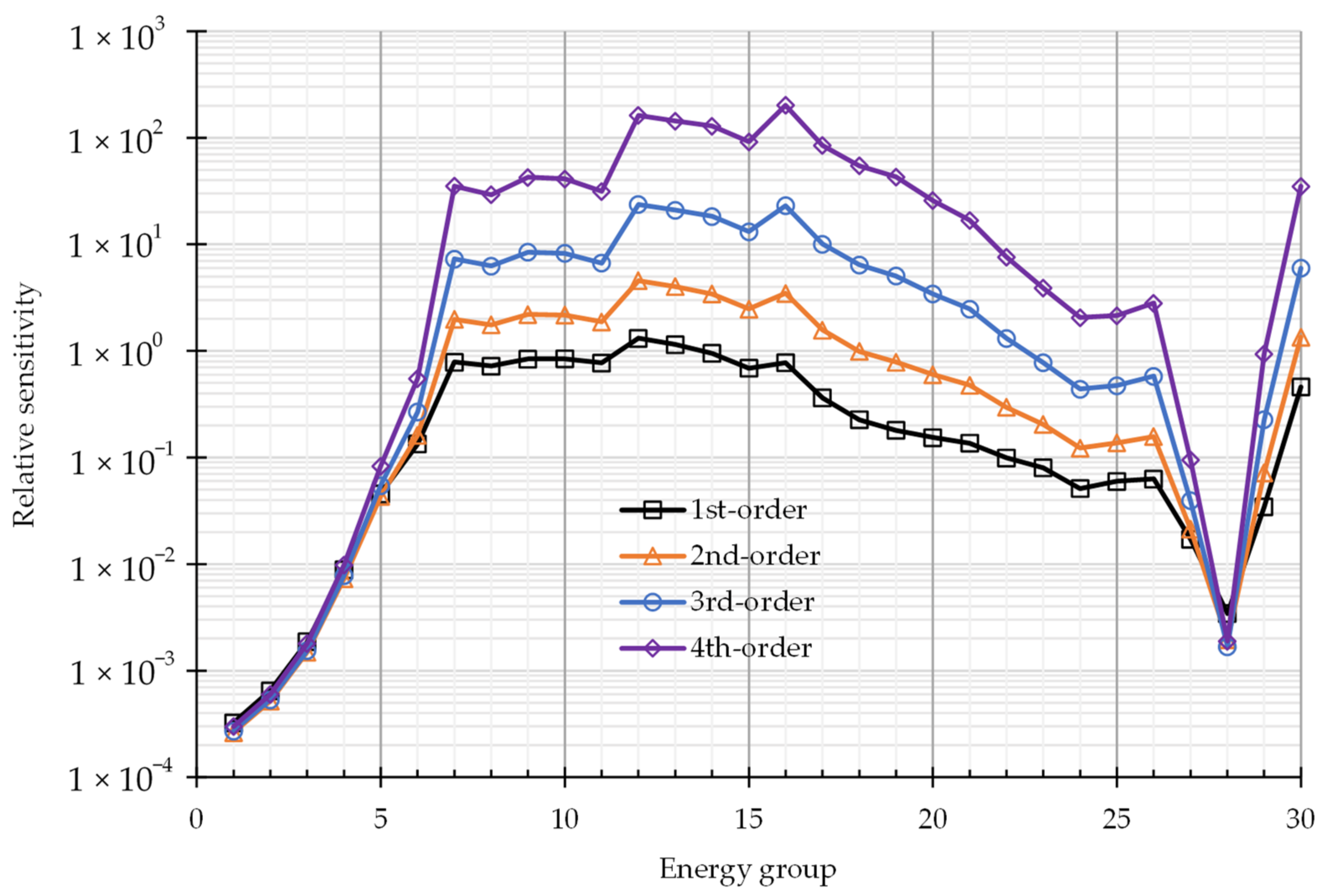
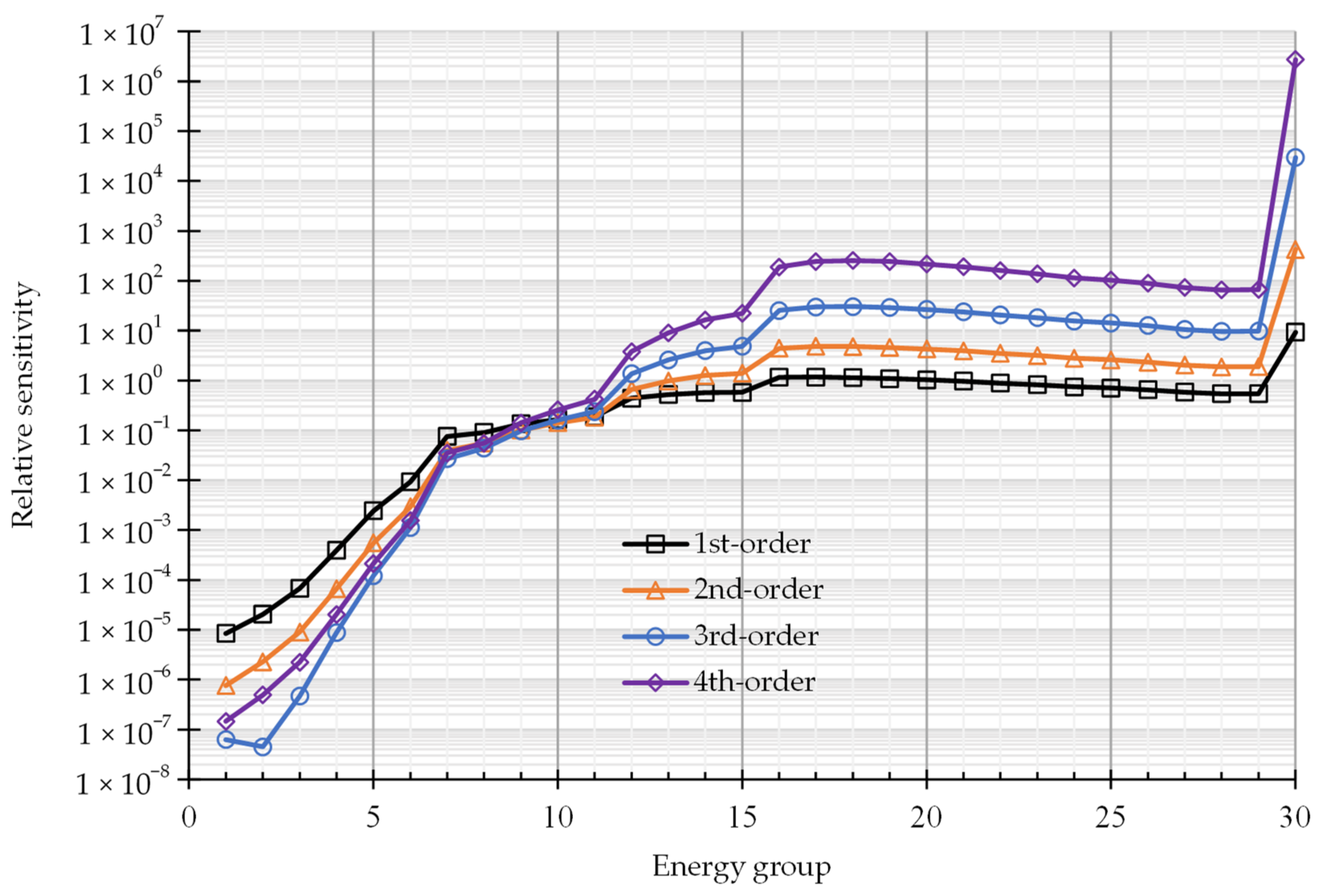
2.1. Numerical Results for Fourth-Order Unmixed Sensitivities and Comparison with the Corresponding 1st-, 2nd- and 3rd-Order Unmixed Sensitivities

S ( 4 ) σ t , i g , σ t , i g , σ t , i g , σ t , i g 4 L / σ t , i g 4 σ t , i g 4 / L , i = 1 , , 6 ; g = 1 , , 30 , represents the 4th-order unmixed relative sensitivities of the PERP leakage response with respect to the same microscopic total cross section (namely: σ t , i g ) for each isotope and for each energy group. These unmixed sensitivities are important since they contribute to the moments (i.e., expected values, variances/covariances, skewness) of the response distribution even when the model parameters are uncorrelated. Moreover, the values of these unmixed 4th-order relative sensitivities of the response to the same model parameters can be directly compared to the values of the corresponding 1st-order, 2nd-order and 3rd-order unmixed relative sensitivities, namely, S ( 1 ) σ t , i g , S ( 2 ) σ t , i g , σ t , i g and S ( 3 ) σ t , i g , σ t , i g , σ t , i g ,   i = 1 , , 6 ; g = 1 , , 30 . These comparisons are presented in Table 2, Table 3, Table 4, Table 5, Table 6 and Table 7 for the six isotopes that are contained in the PERP benchmark. The relative sensitivities which are larger than unity are highlighted using bold numbers.
Table 2 presents a side-by-side comparison of the 4th-order unmixed relative sensitivities to the corresponding 1st-, 2nd- and 3rd-order ones, for all energy groups g = 1 , , 30 , of isotope 1 (239Pu) of the PERP benchmark. Figure 2 further illustrates the comparison of the absolute values of the 1st-order through 4th-order unmixed relative sensitivities for isotope 1 (239Pu) of the PERP benchmark. It shows that the number of 4th-order relative sensitivities that have large absolute values (e.g., greater than 1.0) is far greater than the number of 1st-order, 2nd-order and 3rd-order relative sensitivities that have values greater than 1.0 (as highlighted in bold in this table). Furthermore, the values of the 4th-order relative sensitivities are much larger than the corresponding values of the 1st-, 2nd- and 3rd-order unmixed sensitivities. Specifically, for energy groups g = 7 , , 26 and g = 29 , 30 , the values of the 4th-order relative sensitivities are ca. 3−8 times larger than the corresponding values of the 3rd-order sensitivities, are ca. 12−57 times larger than the corresponding 2nd-order ones, and are ca. 26−259 times larger than the corresponding values of the 1st-order sensitivities. The largest value for the 4th -order unmixed relative sensitivity is S ( 4 ) σ t , 1 g = 16 , σ t , 1 g = 16 , σ t , 1 g = 16 , σ t , 1 g = 16 = 202.03 , which occurs for the 16th energy group. By comparison, the largest values for the 1st-, 2nd-, 3rd-order unmixed relative sensitivities are S ( 1 ) σ t , 1 g = 12 = 1.32 ,   S ( 2 ) σ t , 1 g = 12 , σ t , 1 g = 12 = 4.586 and S ( 3 ) σ t , 1 g = 12 , σ t , 1 g = 12 , σ t , 1 g = 12 = 23.71 , which all occur for the 12th energy group. It is noteworthy that all of the 1st-order and 3rd-order unmixed relative sensitivities are negative, while all of the unmixed 2nd-order and 4th-order ones are positive.
Table 3, Table 4 and Table 5 compare the 4th-order unmixed relative sensitivities with the corresponding 1st-, 2nd- and 3rd-order ones, for isotopes 2, 3 and 4 (namely, 240Pu, 69Ga and 71Ga) of the PERP benchmark, respectively, and all energy groups g = 1 , , 30 . As can be seen from these tables, the values for all of the 1st–4th order unmixed relative sensitivities are very small, i.e., of the order of 10−2 or less. However, for the same energy group of each isotope, the value of the 1st-order relative sensitivity is generally the largest, followed by the 2nd-order sensitivity, and then by the 3rd-order sensitivity, while the 4th-order sensitivity is the smallest. Specifically, as shown in Table 3, for all energy groups (except for groups 27 and 28) of the isotope 240Pu, the values of the 1st-order relative sensitivities are ca. 3–30 times greater than the corresponding values of the 2nd-order sensitivities, ca. 1–2 orders of magnitudes greater than the corresponding values of the 3rd-order ones and ca. 1–3 orders of magnitudes greater than the corresponding values of the 4th-order ones. Similarly, as shown in Table 4 and Table 5, respectively, for all energy groups of isotopes 69Ga and 71Ga, the values of the 1st-order relative sensitivities are ca. 2–3 orders of magnitudes greater than the corresponding values of the 2nd-order sensitivities, and ca. 4–5 orders of magnitudes greater than the corresponding values of the 3rd-order ones, and ca. 5–12 orders of magnitudes greater than the corresponding values of the 4th-order ones. All of the 1st- and 3rd-order unmixed relative sensitivities presented in Table 3, Table 4 and Table 5 are negative, while all the 2nd-order and 4th-order unmixed relative sensitivities are positive.
Table 6 presents a comparison among the values of the 1st-, 2nd-, 3rd- and 4th-order unmixed relative sensitivities for isotope 5 (C). As shown in this table, the sensitivity values are mostly of the order of 10−1 or 10−2 (or less) for all energy groups, except for the lowest energy group (g = 30). For each energy group, g = 1 , , 29 , the 1st-order relative sensitivities are the largest, followed by the 2nd-order sensitivities, while the 3rd-order and 4th-order sensitivities are the smallest, respectively. Specifically, for these groups, the absolute values of the 1st-order relative sensitivities are around one order of magnitude greater than that of the corresponding 2nd-order sensitivities, and the 2nd-order sensitivities are generally 1 to 3 times greater than the corresponding 3rd-order ones, while the magnitudes of the 3rd-order sensitivities are close to the corresponding 4th-order ones. However, for the lowest group (g = 30), all the 1st-, 2nd-, 3rd- and 4th-order unmixed relative sensitivities reach their respective largest values, which are significantly larger than the values in other groups; in particular, the largest 4th-order unmixed sensitivity S ( 4 ) σ t , 5 g = 30 , σ t , 5 g = 30 , σ t , 5 g = 30 , σ t , 5 g = 30 = 134.02 is the overall largest in the table, followed by the largest 3rd-order sensitivity S ( 3 ) σ t , 5 g = 30 , σ t , 5 g = 30 , σ t , 5 g = 30 = 17.45 , the largest 2nd-order sensitivity S ( 2 ) σ t , 5 g = 30 , σ t , 5 g = 30 = 3.01 , and the largest 1st-order sensitivity S ( 1 ) σ t , 5 g = 30 = 0.785 , respectively.
Table 7 and Figure 3 present a comparison of the values of the unmixed relative sensitivities for isotope 6 (1H) from 1st-order through 4th-order. As shown in the table and the figure, many of the relative sensitivities for isotope 6 (1H) have absolute values greater than 1.0, including 6 first-order sensitivities, 17 second-order unmixed sensitivities, 19 third-order unmixed sensitivities, and 19 fourth-order unmixed sensitivities, as highlighted in bold in Table 7. All the sensitivities for energy groups g = 1 , , 11 are relatively small (i.e., of the order of 10−1 or smaller), but the 1st-order sensitivities are slightly larger (in absolute values) than the corresponding 2nd-, 3rd- and 4th-order ones. For energy groups g = 12 , , 29 , all of the 4th-order unmixed relative sensitivities are significantly larger than the corresponding 1st-, 2nd- and 3rd-order ones. Depending on the specific energy group, the values of the 4th-order relative sensitivity are ca. 2 to 7 times larger than the corresponding 3rd-order ones, ca. 5 to 52 times larger than the values of the corresponding 2nd-order sensitivities, and ca. 8 to 220 times larger than the values of the corresponding 1st-order sensitivities. As shown in Table 7, the largest absolute values for the 1st-, 2nd-, 3rd- and 4th-order unmixed relative sensitivities all occur for the lowest-energy group (g = 30; thermal neutrons), which are significantly larger than the values of the sensitivities in other energy groups. Notably, the largest 4th-order unmixed relative sensitivity attains a very large value: S ( 4 ) σ t , 6 g = 30 , σ t , 6 g = 30 , σ t , 6 g = 30 , σ t , 6 g = 30 = 2.720 × 10 6 . By comparison, the largest values for the 1st-, 2nd- and 3rd-order unmixed relative sensitivities are: S ( 1 ) σ t , 6 g = 30 = 9.366 , S ( 2 ) σ t , 6 g = 30 , σ t , 6 g = 30 = 4.296 × 10 2 and S ( 3 ) σ t , 6 g = 30 , σ t , 6 g = 30 , σ t , 6 g = 30 = 2.966 × 10 4 , respectively.
In summary, the results in Table 2, Table 3, Table 4, Table 5, Table 6 and Table 7 indicate that the microscopic total cross sections of isotopes 1H and 239Pu of the PERP benchmark are the most important parameters affecting the PERP benchmark’s leakage response since they are involved in all of the large values (i.e., greater than 1.0) of the 1st-, 2nd-, 3rd- and 4th-order unmixed relative sensitivities. By comparison, as shown in Table 3, Table 4, Table 5 and Table 6, all of the unmixed relative sensitivities that involve the microscopic total cross sections of isotopes 240Pu, 69Ga, 71Ga and C have values of the order of 10−2 or less (with one exception, for isotope 5 in energy g = 30 ). Moreover, the results in Table 2 and Table 7 indicate that, for most energy groups, the values of the 4th-order unmixed relative sensitivities for isotopes 1H and 239Pu are significantly larger than the corresponding values of the 1st-, 2nd- and 3rd-order unmixed sensitivities. In particular, the largest 1st-, 2nd-, 3rd- and 4th-order unmixed sensitivities arise from the microscopic total cross sections σ t , 1 g = 12 and σ t , 1 g = 16 of isotope 1 (239Pu), and σ t , 6 g = 30 of isotope 6 (1H), respectively. Specifically, for isotope 239Pu, as shown in Table 2, the largest 4th-order unmixed relative sensitivity attains a value of S ( 4 ) σ t , 1 g = 16 , σ t , 1 g = 16 , σ t , 1 g = 16 , σ t , 1 g = 16 = 202.03 , which is ca. 8 times larger than the corresponding largest 3rd-order relative sensitivity and ca. 57 times larger than that of the corresponding largest 2nd-order one, and ca. 259 times larger than the corresponding largest 1st-order one. Notably, for isotope 1H, as shown in Table 7, all of the sensitivities have very large values: the largest 4th-order unmixed relative sensitivity has an extremely large value of S ( 4 ) σ t , 6 g = 30 , σ t , 6 g = 30 , σ t , 6 g = 30 , σ t , 6 g = 30 = 2.720 × 10 6 , which is ca. 90 times larger than the corresponding largest 3rd-order relative sensitivity, and ca. 6350 times larger than the corresponding largest 2nd-order one, and ca. 291,000 times larger than the corresponding largest 1st-order relative sensitivity.
In summary, the most important parameters among the 180 microscopic total cross sections of the PERP benchmark are:
(i)
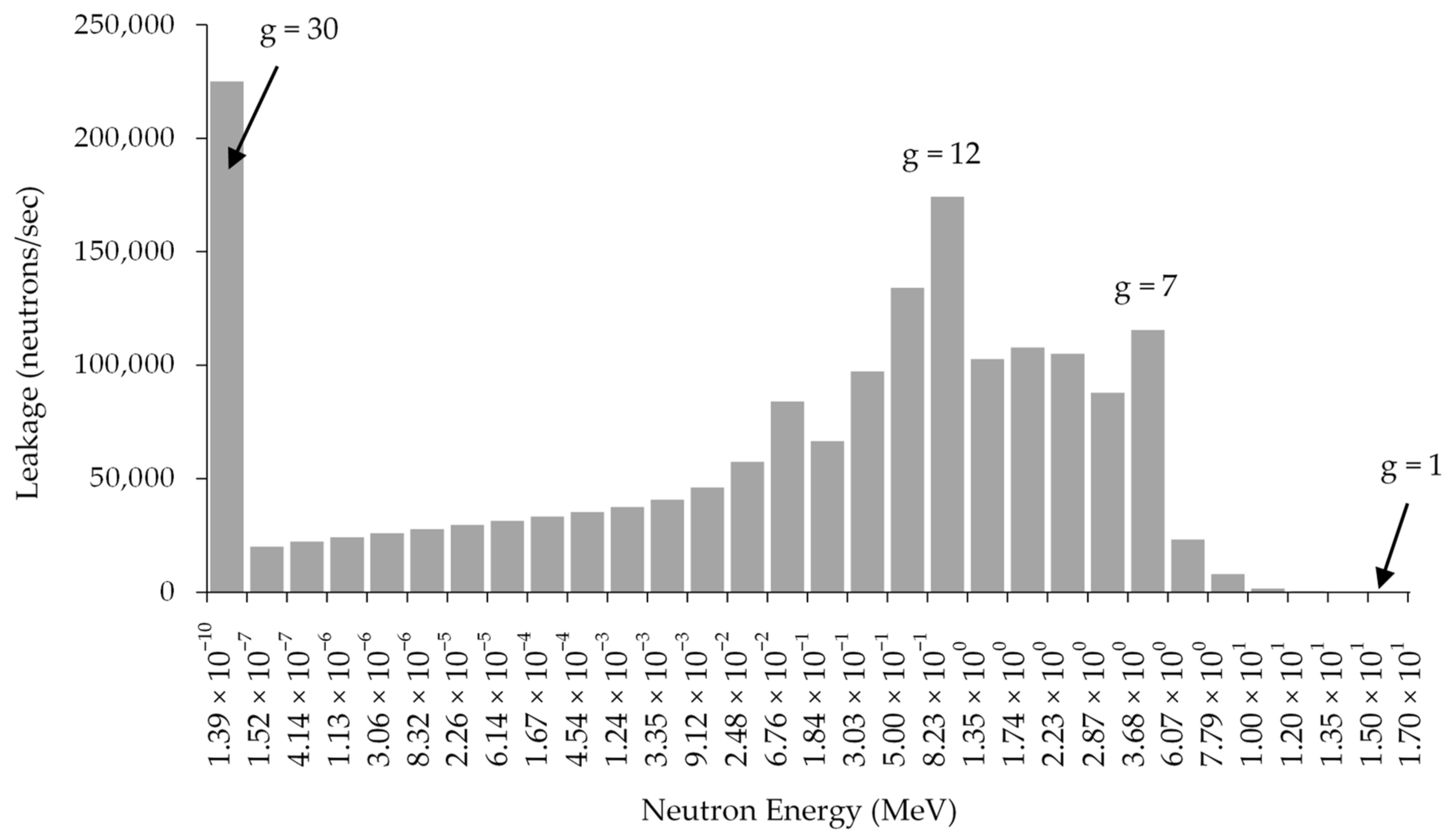
the microscopic total cross section for the 12th-energy group (which comprises the energy interval from 0.823 MeV to 1.35 MeV) and the 16th-energy group (which comprises the energy interval from 67.6 KeV to 184 KeV) of isotope 239Pu (i.e., σ t , 1 g = 12 and σ t , 1 g = 16 ); and
(ii)
the 30th energy group (which comprises thermalized neutrons in the energy interval from 1.39 × 10⁻⁴ eV to 0.152 eV) of isotope 1H (i.e., σ t , 6 30 ).
As illustrated in Figure 1 for the histogram plot of the leakage for each energy group of the PERP benchmark, the largest neutron leakage occurs in group 30, and the 2nd-largest leakage occurs in group 12. It is therefore not surprising that most of the large relative sensitivities are related to the 12th-energy group and the 30th energy group. Furthermore, the 16th-energy group of isotope 239Pu becomes important only for the 4th-order sensitivities, as the largest 4th-order unmixed sensitivity of isotope 1 (239Pu) is with respect to the parameter σ t , 1 g = 16 .
Notably, the results presented in Table 2, Table 3, Table 4, Table 5, Table 6 and Table 7 also indicate that the 1st-order and 3rd-order unmixed relative sensitivities are all negative, while the 2nd-order and 4th-order unmixed relative sensitivities are all positive for all six isotopes contained in the PERP benchmark.

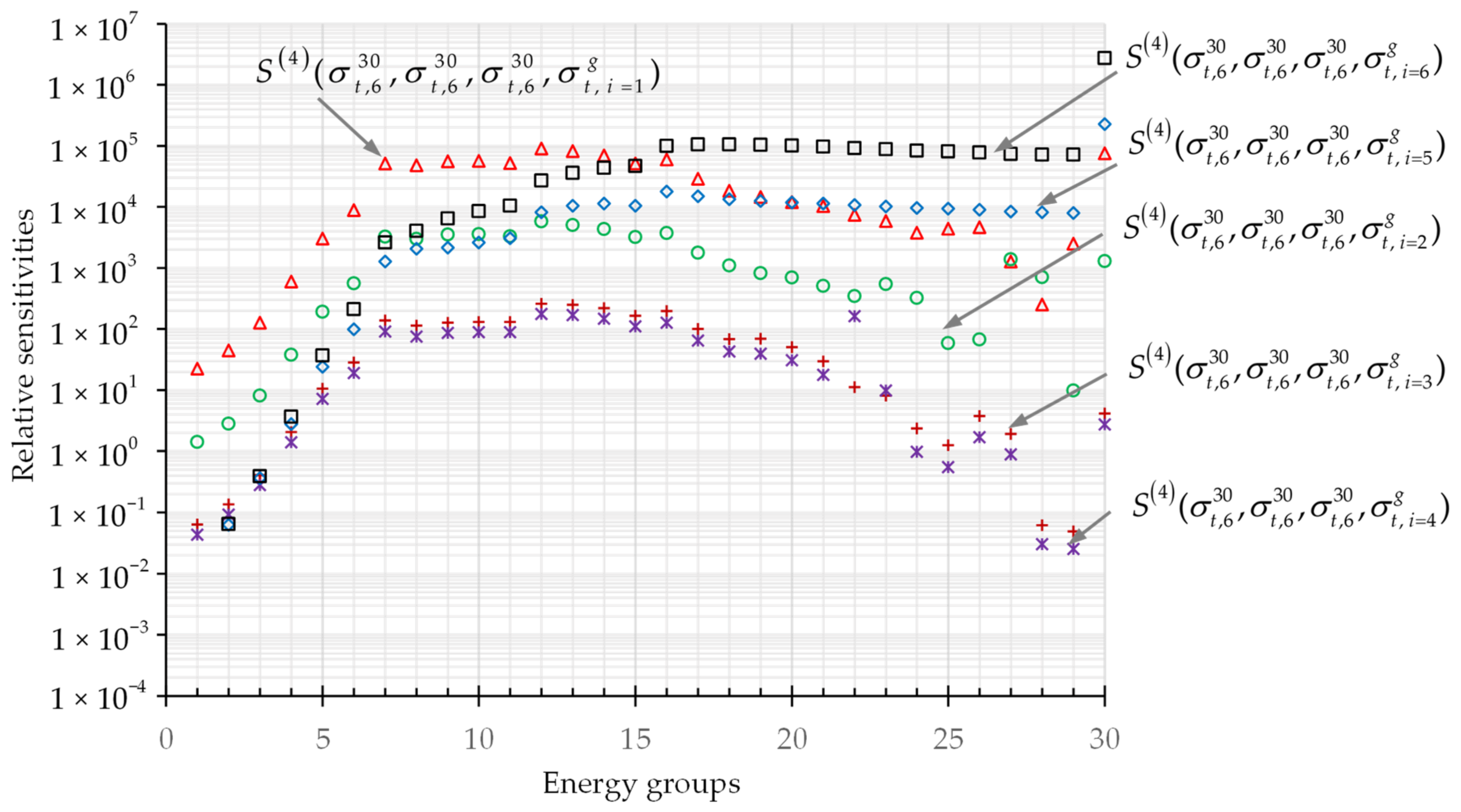
2.2. Numerical Results for Fourth-Order Mixed Sensitivities Corresponding to the Largest Third-Order Sensitivities

The total number of fourth-order sensitivities of the PERP leakage response with respect to the microscopic total cross sections is 1,049,760,000, of which 45,212,895 are distinct. Although it is by far the most efficient method for computing sensitivities, the 4th-CASAM would still need ca. 11,568 h CPU-time, using a DELL computer (AMD FX-8350) with an 8-core processor, for obtaining the exact values of all of the distinct 4th-order sensitivities 4 L α / t j 4 t j 3 t j 2 t j 1 [13]. Therefore, the computation of these sensitivities must be prioritized, and the priority order selected in this work is to compute the ones that are expected to be the largest. Thus, based on the trends indicated by the numerical results presented in Table 2, Table 3, Table 4, Table 5, Table 6 and Table 7, it would be expected that the largest 4th-order sensitivities would be those which correspond to the largest 3rd-order ones. Previous computations [11] of the third-order sensitivities of the PERP leakage response to the benchmark’s microscopic total cross sections indicated that the largest 3rd-order unmixed and mixed sensitivities are S ( 3 ) σ t , 6 g = 30 , σ t , 6 g = 30 , σ t , 6 g = 30 and S ( 3 ) σ t , 1 g 1 = 30 , σ t , 6 g 2 = 30 , σ t , 6 g 3 = 30 , respectively. It was also shown in [11] that the microscopic total cross sections σ t , 1 g = 30 and σ t , 6 30 for the 30th energy group of isotopes 239Pu and 1H are the two most important parameters affecting the PERP benchmark’s leakage response since they are involved in the largest mixed and unmixed 1st-, 2nd- and 3rd-order sensitivities. Therefore, the 4th-order sensitivities of the PERP leakage response corresponding to S ( 3 ) σ t , 6 g = 30 , σ t , 6 g = 30 , σ t , 6 g = 30 and S ( 3 ) σ t , 1 g 1 = 30 , σ t , 6 g 2 = 30 , σ t , 6 g 3 = 30 have been computed with the highest priority. The numerical results for the mixed 4th-order sensitivities corresponding to S ( 3 ) σ t , 6 30 , σ t , 6 30 , σ t , 6 30 are reported in Section 2.2.1, while the numerical results for the 4th-order sensitivities corresponding to the largest 3rd-order mixed sensitivity, namely S ( 3 ) σ t , 1 30 , σ t , 6 30 , σ t , 6 30 , are reported in Section 2.2.2.

2.2.1. Fourth-Order Mixed Sensitivities S ( 4 ) σ t , 6 30 , σ t , 6 30 , σ t , 6 30 , σ t , i g , i = 1 , , 6 ; g = 1 , , 30

Corresponding to the largest unmixed 3rd-order sensitivity S ( 3 ) σ t , 6 30 , σ t , 6 30 , σ t , 6 30 , there are 180 fourth-order mixed sensitivities of the PERP leakage response with respect to the 180 microscopic total cross sections, namely, S ( 4 ) σ t , 6 30 , σ t , 6 30 , σ t , 6 30 , σ t , i g ,   i = 1 , , 6 ;   g = 1 , , 30 . Figure 4 illustrates the numerical results obtained for these 4th-order mixed relative sensitivities by using a distinct symbol and color for each of the isotopes i = 2 , , 6 .
As shown in Figure 4, the majority (i.e., 163 out of 180) of the 4th-order mixed relative sensitivities S ( 4 ) σ t , 6 30 , σ t , 6 30 , σ t , 6 30 , σ t , i g , i = 1 , , 6 ; g = 1 , , 30 , have values greater than 1.0. Generally, the values for S ( 4 ) σ t , 6 30 , σ t , 6 30 , σ t , 6 30 , σ t , i = 1 g and S ( 4 ) σ t , 6 30 , σ t , 6 30 , σ t , 6 30 , σ t , i = 6 g are among the largest, followed by the values for S ( 4 ) σ t , 6 30 , σ t , 6 30 , σ t , 6 30 , σ t , i = 5 g and S ( 4 ) σ t , 6 30 , σ t , 6 30 , σ t , 6 30 , σ t , i = 2 g , while the values for S ( 4 ) σ t , 6 30 , σ t , 6 30 , σ t , 6 30 , σ t , i = 3 g and S ( 4 ) σ t , 6 30 , σ t , 6 30 , σ t , 6 30 , σ t , i = 4 g are among the smallest. This is consistent with the previous observations, which indicated that the microscopic total cross sections of isotopes 1 (239Pu) and 6 (1H) have a larger impact on the sensitivities than the microscopic total cross sections of isotopes 2, 3 and 4 (i.e.,240Pu, 69Ga, and 71Ga). For the highest energy groups, g = 1 , , 6 , which comprise the energy interval from 6.07 MeV to 17.0 MeV, the sensitivities S ( 4 ) σ t , 6 30 , σ t , 6 30 , σ t , 6 30 , σ t , i = 1 g are the largest among the sensitivities corresponding to each of the depicted isotopes. For the lower energy groups g = 7 , , 15 , which comprise the energy interval from 184.0 KeV to 6.07 MeV, the values S ( 4 ) σ t , 6 30 , σ t , 6 30 , σ t , 6 30 , σ t , i = 1 g are also the largest, followed by S ( 4 ) σ t , 6 30 , σ t , 6 30 , σ t , 6 30 , σ t , i = 6 g , S ( 4 ) σ t , 6 30 , σ t , 6 30 , σ t , 6 30 , σ t , i = 5 g and S ( 4 ) σ t , 6 30 , σ t , 6 30 , σ t , 6 30 , σ t , i = 2 g , respectively. For energy groups g = 16 , , 30 , which comprise the energy interval from 1.39 × 10⁻⁴ eV to 184.0 KeV, the values of S ( 4 ) σ t , 6 30 , σ t , 6 30 , σ t , 6 30 , σ t , i = 6 g are the largest, followed by S ( 4 ) σ t , 6 30 , σ t , 6 30 , σ t , 6 30 , σ t , i = 5 g , S ( 4 ) σ t , 6 30 , σ t , 6 30 , σ t , 6 30 , σ t , i = 1 g and S ( 4 ) σ t , 6 30 , σ t , 6 30 , σ t , 6 30 , σ t , i = 2 g , respectively. Figure 4 also indicates that among the 180 fourth-order relative sensitivities S ( 4 ) σ t , 6 30 , σ t , 6 30 , σ t , 6 30 , σ t , i g , i = 1 , , 6 ; g = 1 , , 30 , the overall largest value is attained by the unmixed sensitivity S ( 4 ) σ t , 6 30 , σ t , 6 30 , σ t , 6 30 , σ t , 6 30 = 2.720 × 10 6 , which is presented in Section 2.1. The overall largest mixed 4th-order relative sensitivity is S ( 4 ) σ t , 6 30 , σ t , 6 30 , σ t , 6 30 , σ t , 5 30 = 2.279 × 10 5 , which involves the 30th energy group (thermalized neutrons) of the microscopic total cross sections for isotopes 6 (1H) and 5 (C).

2.2.2. Fourth-Order Mixed Sensitivities S ( 4 ) σ t , 1 30 , σ t , 6 30 , σ t , 6 30 , σ t , i g , i = 1 , , 6 ; g = 1 , , 30

The 180 fourth-order mixed sensitivities, S ( 4 ) σ t , 1 30 , σ t , 6 30 , σ t , 6 30 , σ t , i g , i = 1 , , 6 ; g = 1 , , 30 , which correspond to the largest mixed 3rd-order sensitivity S ( 3 ) σ t , 1 30 , σ t , 6 30 , σ t , 6 30 , are depicted in Figure 5.
As shown in Figure 5, the data distributions for S ( 4 ) σ t , 1 30 , σ t , 6 30 , σ t , 6 30 , σ t , i g , i = 1 , , 6 ; g = 1 , , 30 are very similar to the distributions depicted in Figure 4, except that the magnitudes of the sensitivities for S ( 4 ) σ t , 1 30 , σ t , 6 30 , σ t , 6 30 , σ t , i g , i = 1 , , 6 ; g = 1 , , 30 are ca. two orders smaller than those for S ( 4 ) σ t , 6 30 , σ t , 6 30 , σ t , 6 30 , σ t , i g , i = 1 , , 6 ; g = 1 , , 30 . The majority (i.e., 139 out of 180) of the 4th-order mixed relative sensitivities S ( 4 ) σ t , 1 30 , σ t , 6 30 , σ t , 6 30 , σ t , i g , i = 1 , , 6 ; g = 1 , , 30 have values greater than 1.0. As in Figure 4, the largest sensitivities are S ( 4 ) σ t , 1 30 , σ t , 6 30 , σ t , 6 30 , σ t , i = 1 g and S ( 4 ) σ t , 1 30 , σ t , 6 30 , σ t , 6 30 , σ t , i = 6 g , followed by S ( 4 ) σ t , 1 30 , σ t , 6 30 , σ t , 6 30 , σ t , i = 5 g and S ( 4 ) σ t , 1 30 , σ t , 6 30 , σ t , 6 30 , σ t , i = 2 g , while the values for S ( 4 ) σ t , 1 30 , σ t , 6 30 , σ t , 6 30 , σ t , i = 3 g and S ( 4 ) σ t , 1 30 , σ t , 6 30 , σ t , 6 30 , σ t , i = 4 g are generally the smallest. The overall largest value in S ( 4 ) σ t , 1 30 , σ t , 6 30 , σ t , 6 30 , σ t , i g , i = 1 , , 6 ; g = 1 , , 30 , is attained by S ( 4 ) σ t , 1 30 , σ t , 6 30 , σ t , 6 30 , σ t , 6 30 = 7.561 × 10 4 , which involves the 30th energy group of the microscopic total cross sections for isotopes 1 (239Pu) and 6 (1H).

3. Verification of the 4th-Order Mixed Relative Sensitivities

Within the 4th-CASAM, the 2nd-order mixed sensitivities are computed twice, using two distinct expressions that involve two distinct 2nd-level adjoint functions. Therefore, the 4th-CASAM provides an independent way for verifying the 2nd-order mixed sensitivities by using their inherent symmetries. In the same way, the 4th-CASAM provides six distinct expressions, involving four distinct 3rd-level adjoint functions, for the computation of the 3rd-order mixed sensitivities, so the correctness and accuracy of their computations (and, therefore, the accuracy of the computations of the underlying adjoint functions) is inherently assured within the 4th-CASAM by ensuring that each set of symmetric sensitivities has the same numerical value. Finally, the 4th-CASAM provides 24 distinct expressions, involving eight distinct 4th-level adjoint functions, for the computation of the 4th-order mixed sensitivities, so the correctness and accuracy of their computations are inherently assured within the 4th-CASAM by ensuring that each set of symmetric sensitivities has the same numerical value, within small round-off errors.
On the other hand, the unmixed sensitivities (of all orders) are computed within the 4th-CASAM just once since the unmixed sensitivities do not possess symmetries inherent in the mixed sensitivities. Thus, the unmixed sensitivities can be verified within the 4th-CASAM framework only indirectly, since the adjoint functions which enter in the expressions of the unmixed sensitivities also enter in the expressions of the corresponding mixed ones, so they will have been verified within the intrinsic 4th-CASAM verification process based on the symmetries of the mixed sensitivities. The only way to verify the unmixed sensitivities directly and without involving adjoint functions in their verification process is to compute them approximately by using finite-difference formulas in conjunction with forward re-calculations and compare the numerical values obtained using finite-differences with the values produced by the 4th-CASAM. However, as will be illustrated in Section 4 below, this comparison process is not self-evident since the values produced by the finite-difference schemes are seldom accurate. Furthermore, the accuracy of the finite-difference formulas for higher-order derivatives/sensitivities becomes increasingly more sensitive to the chosen step-size.

3.1. Exact Verification of the 4th-Order Mixed Sensitivities Using the Inherent Symmetries within the 4th-CASAM

For the 4th-order mixed sensitivities of the leakage response with respect to four different parameters, there are six sets of symmetrical sensitivities, each set comprising four symmetrical sensitivities that have the same numerical value. Altogether, the following 24 absolute sensitivities are symmetrical: 4 L α / α j 1 α j 2 α j 3 α j 4 , 4 L α / α j 1 α j 2 α j 4 α j 3 , 4 L α / α j 1 α j 3 α j 2 α j 4 , 4 L α / α j 1 α j 3 α j 4 α j 2 , 4 L α / α j 1 α j 4 α j 2 α j 3 , 4 L α / α j 1 α j 4 α j 3 α j 2 , 4 L α / α j 2 α j 1 α j 3 α j 4 , 4 L α / α j 2 α j 1 α j 4 α j 3 , 4 L α / α j 2 α j 3 α j 1 α j 4 , 4 L α / α j 2 α j 3 α j 4 α j 1 , 4 L α / α j 2 α j 4 α j 1 α j 3 , 4 L α / α j 2 α j 4 α j 3 α j 1 , 4 L α / α j 3 α j 1 α j 2 α j 4 , 4 L α / α j 3 α j 1 α j 4 α j 2 , 4 L α / α j 3 α j 2 α j 1 α j 4 , 4 L α / α j 3 α j 2 α j 4 α j 1 , 4 L α / α j 4 α j 2 α j 1 α j 3 , 4 L α / α j 4 α j 2 α j 3 α j 1 , 4 L α / α j 4 α j 1 α j 2 α j 3 , 4 L α / α j 4 α j 1 α j 3 α j 2 , 4 L α / α j 4 α j 2 α j 1 α j 3 , 4 L α / α j 4 α j 2 α j 3 α j 1 , 4 L α / α j 4 α j 3 α j 1 α j 2 , 4 L α / α j 4 α j 3 α j 2 α j 1 . Each of these 24 sensitivities can be independently computed using distinct expressions, involving distinct 2nd-, 3rd- and 4th-level adjoint systems and the corresponding adjoint functions ψ i 2 j 1 ; r , Ω , i = 1 , 2 ;   ψ i 3 j 2 ; j 1 ; r , Ω , i = 1 , , 4 , and ψ i 4 j 3 ; j 2 ; j 1 ; r , Ω , i = 1 , , 8 . The numerical values of these 24 mixed sensitivities can be verified by intercomparisons, thus providing a mutual “solution verification” that the respective computations were performed correctly.
As an example, corresponding to the overall largest 4th-order mixed relative sensitivity S ( 4 ) σ t , 6 30 , σ t , 6 30 , σ t , 6 30 , σ t , 5 30 = 2.279 × 10 5 , as shown in Figure 4, there are three symmetric ones, namely: S ( 4 ) σ t , 6 30 , σ t , 6 30 , σ t , 5 30 , σ t , 6 30 = 2.279 × 10 5 , S ( 4 ) σ t , 6 30 , σ t , 5 30 , σ t , 6 30 , σ t , 6 30 = 2.279 × 10 5 , and S ( 4 ) σ t , 5 30 , σ t , 6 30 , σ t , 6 30 , σ t , 6 30 = 2.279 × 10 5 . Each of them was solved independently using the 4th-CASAM method, and their values are identical for this example.
As a further illustrative example, consider the largest 4th-order mixed relative sensitivity depicted in Figure 5, which is the 4th-order mixed sensitivity of the leakage response with respect to the parameters σ t , 1 30 , σ t , 6 30 , σ t , 6 30 and σ t , 6 30 , i.e., S ( 4 ) σ t , 1 30 , σ t , 6 30 , σ t , 6 30 , σ t , 6 30 = 7.561 × 10 4 , which occurs for group 30 of isotope 1 (239Pu) and isotope 6 (1H). Comparing S ( 4 ) σ t , 1 30 , σ t , 6 30 , σ t , 6 30 , σ t , 6 30 = 7.561 × 10 4 to the corresponding symmetric sensitivities, namely: S ( 4 ) σ t , 6 30 , σ t , 1 30 , σ t , 6 30 , σ t , 6 30 = 7.556 × 10 4 , S ( 4 ) σ t , 6 30 , σ t , 6 30 , σ t , 1 30 , σ t , 6 30 = 7.556 × 10 4 and S ( 4 ) σ t , 6 30 , σ t , 6 30 , σ t , 6 30 , σ t , 1 30 = 7.550 × 10 4 , indicates that these sensitivities agree well with each other. The small numerical differences between these sensitivities stem from small numerical differences in the numerical values for the forward and various adjoint functions, which are computed using the PARTISN code [14].
A similar verification was performed for the 4th-order mixed sensitivity S ( 4 ) σ t , 1 30 , σ t , 1 30 , σ t , 6 30 , σ t , 6 30 = 3.739 × 10 3 of the leakage response with respect to the parameters σ t , 1 30 , σ t , 1 30 , σ t , 6 30 and σ t , 6 30 . The corresponding symmetric sensitivities are: S ( 4 ) σ t , 1 30 , σ t , 6 30 , σ t , 6 30 , σ t , 1 30 = 3.742 × 10 3 , S ( 4 ) σ t , 1 30 , σ t , 6 30 , σ t , 1 30 , σ t , 6 30 = 3.739 × 10 3 , S ( 4 ) σ t , 6 30 , σ t , 1 30 , σ t , 6 30 , σ t , 1 30 = 3.735 × 10 3 and S ( 4 ) σ t , 6 30 , σ t , 6 30 , σ t , 1 30 , σ t , 1 30 = 3.735 × 10 3 , which also agree very well among each other. These verifications provide confidence in the computations of the sensitivities themselves and also in the numerical computations of the various adjoint functions which are used for computing efficiently and exactly the corresponding sensitivities.

3.2. Approximate Verification of the 4th-Order Mixed Sensitivities Using Finite-Differences

The well-known finite-difference formula for the 4th-order mixed absolute sensitivities has the following form:
4 L α α j 1 α j 2 α j 3 α j 4 1 16 h j 1 h j 2 h j 3 h j 4 L j 1 + 1 , j 2 + 1 , j 3 + 1 , j 4 + 1 L j 1 + 1 , j 2 + 1 , j 3 + 1 , j 4 1 L j 1 + 1 , j 2 + 1 , j 3 1 , j 4 + 1 + L j 1 + 1 , j 2 + 1 , j 3 1 , j 4 1 L j 1 + 1 , j 2 1 , j 3 + 1 , j 4 + 1 + L j 1 + 1 , j 2 1 , j 3 + 1 , j 4 1 + L j 1 + 1 , j 2 1 , j 3 1 , j 4 + 1 L j 1 + 1 , j 2 1 , j 3 1 , j 4 1 L j 1 1 , j 2 + 1 , j 3 + 1 , j 4 + 1 + L j 1 1 , j 2 + 1 , j 3 + 1 , j 4 1 + L j 1 1 , j 2 + 1 , j 3 1 , j 4 + 1 L j 1 1 , j 2 + 1 , j 3 1 , j 4 1 + L j 1 1 , j 2 1 , j 3 + 1 , j 4 + 1 L j 1 1 , j 2 1 , j 3 + 1 , j 4 1 L j 1 1 , j 2 1 , j 3 1 , j 4 + 1 + L j 1 1 , j 2 1 , j 3 1 , j 4 1 + O h j 1 2 , h j 2 2 , h j 3 2 , h j 4 2 ,
where L j 1 + 1 , j 2 + 1 , j 3 + 1 , j 4 + 1 L α j 1 + h j 1 , α j 2 + h j 2 , α j 3 + h j 3 , α j 4 + h j 4 , etc. In general, finite-difference methods produce only approximate values for the respective derivatives (sensitivities). In particular, the finite-difference formula shown in Equation (7) is subject to second-order errors. For the verification of 4 L α / t j 1 t j 2 3 , the general finite-difference formula for the 4th-order mixed absolute sensitivities given in Equation (7) takes the following form:
4 L α t j 1 t j 2 3 1 16 h j 1 h j 2 3 L j 1 + 1 , j 2 + 3 3 L j 1 + 1 , j 2 + 1 + 3 L j 1 + 1 , j 2 1     L j 1 + 1 , j 2 3 L j 1 1 , j 2 + 3 + 3 L j 1 1 , j 2 + 1 3 L j 1 1 , j 2 1 + L j 1 1 , j 2 3 ,
where L j 1 + 1 , j 2 + 3 L t j 1 + h j 1 , t j 2 + 3 h j 2 , L j 1 1 , j 2 3 L t j 1 h j 1 , t j 2 3 h j 2 , etc., and where h j 1 denotes a variation in the parameter t j 1 around its nominal value t j 1 0 and h j 2 denotes a variation in the parameter t j 2 around its nominal value t j 2 0 .
Two representative 4th-order mixed relative sensitivities were chosen for verification, as follows:
(i)
the largest 4th-order mixed relative sensitivity depicted in Figure 4, i.e., S ( 4 ) σ t , 6 30 , σ t , 6 30 , σ t , 6 30 , σ t , 5 30 = 2.279 × 10 5 , for the leakage response with respect to the microscopic total cross sections for group 30 of isotopes 5 (C) and 6 (1H); and
(ii)
the largest 4th-order mixed relative sensitivity depicted in Figure 5, i.e., S ( 4 ) σ t , 1 30 , σ t , 6 30 , σ t , 6 30 , σ t , 6 30 = 7.561 × 10 4 , which occurs for group 30 of isotopes 1 (239Pu) and 6 (1H).
The trials using various step sizes (i.e., parameter variations) in the finite difference formula provided in Equation (8) for the largest sensitivity, i.e., S ( 4 ) σ t , 6 30 , σ t , 6 30 , σ t , 6 30 , σ t , 5 30 = 2.279 × 10 5 , are presented in Table 8, below. For the finite difference (FD) method, it has been noticed that this method for computing the 4th-order sensitivities is extremely sensitive to the variation of step sizes: when the variations of h j 1 and h j 2 are too large or too small, the results produced by Equation (8) will be far off from the exact value obtained from the 4th-CASAM method.
As shown in Table 8, for a 0.125% change in both parameters σ t , 5 g = 30 and σ t , 6 g = 30 , the finite difference method causes an error of 34.6% from the exact value of S ( 4 ) σ t , 6 30 , σ t , 6 30 , σ t , 6 30 , σ t , 5 30 = 2.279 × 10 5 . The combination of a 0.5% change in σ t , 5 g = 30 and a 0.25% change in σ t , 6 g = 30 reduces the error to 6.34%, which yields the best trial result, as highlighted with bold numbers in the table. However, a 1.0% change in both parameters σ t , 5 g = 30 and σ t , 6 g = 30 increases the error to 197%; the combination of a 3.0% change in σ t , 5 g = 30 and a 1.0% change in σ t , 6 g = 30 further increases the error to 832%. For any combination of h j 1 > 3 % × σ t , 5 30 and h j 2 > 2 % × σ t , 6 30 , the 4th-order mixed sensitivity cannot be computed using the finite difference formula provided in Equation (8), because the PARTISN forward computation fails to converge when computing the last term in Equation (8), namely, L j 1 1 , j 2 3 L t j 1 h j 1 , t j 2 3 h j 2 .
Table 9 presents the results for the trials using various step sizes in the finite difference formula provided in Equation (8) for the largest 4th-order mixed relative sensitivity depicted in Figure 5, which is S ( 4 ) σ t , 1 30 , σ t , 6 30 , σ t , 6 30 , σ t , 6 30 = 7.561 × 10 4 . As shown in Table 9, for a 0.05% change in both parameters σ t , 1 g = 30 and σ t , 6 g = 30 , the finite difference method causes a very large error of 5659% by comparison to the exact value S ( 4 ) σ t , 1 30 , σ t , 6 30 , σ t , 6 30 , σ t , 6 30 = 7.561 × 10 4 . A 0.125% change in both parameters σ t , 1 g = 30 and σ t , 6 g = 30 reduces the error to −0.44%, which yields the smallest error among the various trails, as highlighted by the bold numbers in Table 9. The combination of step-sizes h j 1 = 0.5 % × σ t , 1 30 and h j 2 = 0.25 % × σ t , 6 30 yields an error of −1.10%, which is also very close to the exact value. However, further increasing the step-sizes for h j 1 and h j 2 causes the errors to increase. For instance, a 0.5% change in both parameters σ t , 1 g = 30 and σ t , 6 g = 30 increases the error to 22.9%; a 1.0% change in both parameters σ t , 1 g = 30 and σ t , 6 g = 30 increases the error to −124%; the combination of 3.0% change in σ t , 1 g = 30 and 1.0% change in σ t , 6 g = 30 increases the error to a very large value of 5204%. Any combination of h j 1 > 3 % × σ t , 1 30 and h j 2 > 2 % × σ t , 6 30 , causes the PARTISN forward computation of the last term in Equation (8), L j 1 1 , j 2 3 L t j 1 h j 1 , t j 2 3 h j 2 , to diverge, so the 4th-order mixed sensitivity S ( 4 ) σ t , 1 30 , σ t , 6 30 , σ t , 6 30 , σ t , 6 30 cannot be obtained by using the “second-order accurate” finite difference formula provided in Equation (8).

4. Finite-Difference Computations of the 4th-Order Unmixed Relative Sensitivities

As has been discussed in Section 3 above, the unmixed sensitivities do not possess the symmetries inherent in the mixed sensitivities, so they can be verified within the 4th-CASAM framework only indirectly, via verification of the accuracy of the adjoint functions which enter in their expressions. The only independent means of verifying the unmixed sensitivities is to compute them approximately by using finite-difference formulas in conjunction with forward re-calculations using “judiciously altered” parameter values. The following finite-difference formula is the simplest formula for computing 4th-order unmixed sensitivities, being accurate to second-order errors in the step-size h j :
4 L α α j 4 1 h j 4 L j + 2 4 L j + 1 + 6 L j 4 L j 1 + L j 2 + O h j 2 , j = 1 , , T P ,
where L j + 2 L α j + 2 h j , L j + 1 L α j + h j , L j 1 L α j h j , L j 2 L α j 2 h j , and where the value of the variation h j must be chosen by “trial and error” for each parameter α j .
Two representative 4th-order unmixed relative sensitivities were selected to illustrate the use of the finite-difference formula provided in Equation (9), namely:
(i)
the overall largest 4th-order unmixed relative sensitivity, namely, S ( 4 ) σ t , 6 g = 30 , σ t , 6 g = 30 , σ t , 6 g = 30 , σ t , 6 g = 30 = 2.720 × 10 6 , which occurs for group 30 of isotope 6 (1H);
(ii)
the largest 4th-order unmixed relative sensitivity shown in Table 2, which is the sensitivity S ( 4 ) σ t , 1 g = 16 , σ t , 1 g = 16 , σ t , 1 g = 16 , σ t , 1 g = 16 = 2.020 × 10 2 of the leakage response with respect to the microscopic total cross section for group 16 of isotope 1 (239Pu).
For the computation of S ( 4 ) σ t , 6 g = 30 , σ t , 6 g = 30 , σ t , 6 g = 30 , σ t , 6 g = 30 using Equation (9), several trials were performed using various step-sizes h j , ranging from 0.125% to 2% of σ t , 6 g = 30 . The results of these trials are summarized in Table 10, below.
As shown in Table 10, when using a step-size equal to a 0.125% change in the microscopic total cross section σ t , 6 g = 30 , the finite difference method causes an error of ca. 6010 % by comparison to the exact value S ( 4 ) σ t , 6 g = 30 , σ t , 6 g = 30 , σ t , 6 g = 30 , σ t , 6 g = 30 = 2.720 × 10 6 obtained using the 4th-CASAM method. However, for a 0.5% change in σ t , 6 g = 30 , the error is reduced to −17.7%. The smallest error between the FD-formula and the exact result produced by the 4th-CASAM were attained using a 0.60% change in σ t , 6 g = 30 ; the error was just −0.45%, as highlighted by the bold numbers in the table. On the other hand, a 1.0% change in σ t , 6 g = 30 increased the error to 31.4%, while a 2.0% change in σ t , 6 g = 30 further increased the error of the FD-formula (by comparison to the exact result produced by the 4th-CASAM) to 698%. For h j > 2.5 % × σ t , 6 30 , the PARTISAN forward re-computation did not converge.
Similarly, Table 11 shows comparisons of the value produced by the 4th-CASAM for S ( 4 ) σ t , 1 g = 16 , σ t , 1 g = 16 , σ t , 1 g = 16 , σ t , 1 g = 16 versus the values produced for this sensitivity using the finite difference formula provided in Equation (9). After several trials, it was found that using the value h j = 3.0 % × σ t , 1 g = 16 in Equation (9) yields a value of 205.7 for S ( 4 ) σ t , 1 g = 16 , σ t , 1 g = 16 , σ t , 1 g = 16 , σ t , 1 g = 16 , which is the best finite-difference approximation, just 1.8% away from the exact value S ( 4 ) σ t , 1 g = 16 , σ t , 1 g = 16 , σ t , 1 g = 16 , σ t , 1 g = 16 = 202.03 obtained using the 4th-CASAM method, as highlighted using bold numbers in Table 11. The results provided in Table 11 also indicate that for a small step size of h j = 0.5 % × σ t , 1 g = 16 , the value obtained from the FD-method is ca. −2695% away from the exact value, while for a large step size of h j = 10 % × σ t , 1 g = 16 , the FD-method causes a 30.1% error by comparison to the exact value.

5. Comparison of Computational Requirements for the 4th-Order Sensitivities

Using a DELL computer (AMD FX−8350) with an 8-core processor, the CPU-time for a typical adjoint computation using PARTISN with an angular quadrature of S32 is ca. 24 s, and the CPU-time for computing the integrals over the various adjoint functions which appear in the definition of the respective sensitivity in Equation (2) is ca. 0.004 s. The CPU-time for a typical PARTISN forward computation with an angular quadrature of S32 is ca. 45 s. Thus, the computational times needed for obtaining all of the distinct 1st-, 2nd-, 3rd- and 4th-order sensitivities of the PERP leakage response with respect to the 180 microscopic total cross sections using the 4th-CASAM are as follows:
(i)
To compute the 180 first-order sensitivities, one adjoint PARTISN large-scale computation is needed in order to obtain the 1st-level adjoint function ψ 1 r , Ω . Thus, the CPU-time needed is ca. 24 s [for computing ψ 1 ] plus ca. 1 s for computing the integrals over this adjoint function. By comparison, ca. 270 min are needed to compute these 1st-order sensitivities using the FD-formula.
(ii)
To compute the 180 180 + 1 / 2 = 16 , 290 distinct second-order sensitivities, 180 × 2 = 360 adjoint PARTISN large-scale computations are needed to obtain the 2nd-level adjoint functions ψ 1 2 j 1 ; r , Ω and ψ 2 2 j 1 ; r , Ω , j 1 = 1 , , 180 . Thus, the CPU-time needed is ca. 2.4 h [for computing ψ 1 2 j 1 ; r , Ω and ψ 2 2 j 1 ; r , Ω , j = 1 , , 180 ] plus ca. 3 min for computing the integrals over these adjoint functions. By comparison, ca. 810 h are needed to compute these 2nd-order sensitivities using the FD-formula.
(iii)
To compute the 180 180 + 1 180 + 2 / 3 ! = 988 , 260 distinct third-order sensitivities, 32,940 adjoint PARTISN large-scale computations are needed to obtain the 3rd-level adjoint functions ψ i 3 j 1 ; j 2 ; r , Ω , i = 1 , , 4 ; j 1 , j 2 = 1 , , 180 . Thus, the CPU-time needed is ca. 220 h [for computing ψ i 3 j 1 ; j 2 ; r , Ω , i = 1 , , 4 ; j 1 , j 2 = 1 , , 180 ] plus ca. 0.6 h for computing the integrals over these adjoint functions. By comparison, 98,817 h are needed to compute these 3rd-order sensitivities using the FD-formula.
(iv)
To compute the 180 180 + 1 180 + 2 180 + 3 / 4 ! = 45 , 212 , 985 distinct fourth-order sensitivities, 2,042,040 adjoint PARTISN large-scale computations are needed to obtain the 4th-level adjoint functions ψ i 4 j 1 ; j 2 ; j 3 ; r , Ω , i = 1 , , 8 ; j 1 , j 2 , j 3 = 1 , , 180 . Thus, the CPU-time needed is ca. 25,525 h [for computing ψ i 4 j 1 ; j 2 ; j 3 ; r , Ω , i = 1 , , 8 ; j 1 , j 2 , j 3 = 1 , , 180 ] plus ca. 50 h for computing the integrals over these adjoint functions. By comparison, ca. 1015 years are needed to compute these 4th-order sensitivities using the FD-formula.

6. Conclusions

By applying the 4th-CASAM expression developed in [13], this work has presented the numerical results for the most important 4th-order sensitivities of the PERP benchmark’s leakage response with respect to the benchmark’s microscopic group total cross sections, including 180 4th-order unmixed sensitivities and 360 4th-order mixed sensitivities corresponding to the largest 3rd-order sensitivities. The magnitudes of the 4th-order sensitivities were compared with the corresponding 1st-, 2nd- and 3rd-order ones. In addition, the numerical results obtained for the 4th-order sensitivities were independently verified with the values obtained using the 4th-order finite difference method, as well as with the values of the corresponding symmetric sensitivities. The following conclusions can be drawn from the results reported in this work:
(1)
The number of 4th-order unmixed relative sensitivities that have large values (e.g., greater than 1.0) is far greater than the number of large 1st-, 2nd- and 3rd-order sensitivities. The majority of the large sensitivities involve the isotopes 1H and 239Pu of the PERP benchmark, as shown in Table 2 and Table 7.
(2)
All of the important 4th-order relative sensitivities of the PERP leakage response with respect to the microscopic total cross sections have positive values. By comparison, all of the important 1st-order and 3rd-order relative sensitivities have negative values, while all of the important 2nd-order relative sensitivities have positive values.
(3)
For most energy groups for isotopes 1H and 239Pu, the values of the 4th-order unmixed relative sensitivities are significantly larger than the corresponding values of the 1st-, 2nd- and 3rd-order unmixed sensitivities. The overall largest 4th-order unmixed relative sensitivity is S ( 4 ) σ t , 6 g = 30 , σ t , 6 g = 30 , σ t , 6 g = 30 , σ t , 6 g = 30 = 2.720 × 10 6 , which is around 291,000 times, 6350 times and 90 times larger than the corresponding largest 1st-order, 2nd-order and 3rd-order sensitivities, respectively.
(4)
All of the 1st-order through 4th-order unmixed relative sensitivities that involve the microscopic total cross sections of isotopes 240Pu, 69Ga, 71Ga and C have values of the order of 10−2 or less (except for isotope C at g = 30). For each of these isotopes, within the same energy group, the value of the 1st-order relative sensitivity is generally the largest, followed by the 2nd-order and 3rd-order sensitivities, while the 4th-order sensitivity is the smallest.
(5)
The majority of the 180 4th-order mixed relative sensitivities S ( 4 ) σ t , 6 30 , σ t , 6 30 , σ t , 6 30 , σ t , i g , i = 1 , , 6 ; g = 1 , , 30 , which correspond to the largest unmixed 3rd-order sensitivity S ( 3 ) σ t , 6 30 , σ t , 6 30 , σ t , 6 30 , have values greater than 1.0. Moreover, the mixed sensitivities S ( 4 ) σ t , 6 30 , σ t , 6 30 , σ t , 6 30 , σ t , i = 1 g and S ( 4 ) σ t , 6 30 , σ t , 6 30 , σ t , 6 30 , σ t , i = 6 g , which involve the microscopic total cross sections of isotopes 1 (239Pu) and 6 (1H), are larger than those involving the microscopic total cross sections of isotopes 2, 3 and 4 (i.e.,240Pu, 69Ga, and 71Ga).
(6)
The overall largest mixed 4th-order relative sensitivity is S ( 4 ) σ t , 6 30 , σ t , 6 30 , σ t , 6 30 , σ t , 5 30 = 2.279 × 10 5 , involving the microscopic total cross sections for isotope 6 (1H) and isotope 5 (C) in the 30th energy (thermalized neutrons) group. The sensitivity S ( 4 ) σ t , 6 30 , σ t , 6 30 , σ t , 6 30 , σ t , 5 30 = 2.279 × 10 5 is much larger than the largest 2nd-order and 3rd-order mixed sensitivities.
(7)
The numerical results obtained using the 4th-CASAM for the sensitivities 4 L α / α j 4 and 4 L α / α j 1 α j 2 α j 3 α j 4 have been compared with the results obtained for these quantities by using finite difference formulas that were accurate to the second-order in the respective step-size(s). The finite-difference formulas turned out to be extremely sensitive to the step-size: when the step-sizes were too large or too small, the results produced by the finite-difference formulas were far off from the exact values of the derivatives 4 L α / α j 4 and 4 L α / α j 1 α j 2 α j 3 α j 4 . This finding further highlights the importance of the 4th-CASAM framework for computing accurately and efficiently the 1st-, 2nd-, 3rd-, and 4th-order sensitivities of model responses with respect to model parameters.
Subsequent work [17] will use the 4th-order sensitivity results obtained in this work to perform a 4th-order uncertainty analysis of the PERP benchmark’s leakage response. The impact of the 4th-order sensitivities on the PERP leakage response’s expected value and variance will be compared [17] to the corresponding impact stemming from the corresponding 1st-, 2nd- and 3rd-order sensitivities.
The formulas presented in this work for computing the 4th-order sensitivities of the leakage response to the benchmark’s cross sections, along with the formulas presented in [3,4,5,6,7,8,9,10,11,12,13] for computing the 1st-, 2nd- and 3rd-order sensitivities of the PERP benchmark to cross sections can be implemented in both deterministic and Monte-Carlo codes for solving the neutron transport equations. These formulas could be used for sensitivity analysis of reaction-rate responses in subcritical reactors and for subsequent quantification of uncertainties induced in such responses by the uncertainties in the underlying cross sections. The 4th-order sensitivity analysis methodology used to produce the results presented in this work, along with the previous sensitivity analysis results reported in [3,4,5,6,7,8,9,10,11,12,13], cannot be obtained by any other methods. The computational times that would be required even by simple-minded finite-difference schemes have been shown to be prohibitive for problems involving as many parameters (21,976) as involved in the PERP benchmark. Statistical methods, e.g., based on Latin hypercubes and/or Monte-Carlo, simply cannot produce the results obtained by applying the 4th-order adjoint sensitivity analysis method for large-scale systems, since statistical methods require order-of-magnitude more computations than the simple finite-difference schemes (which already need inordinate amounts of CPU-time). While statistical (e.g., Latin hypercube and/or Monte-Carlo) methods will always produce “numbers,” the adjoint sensitivity analysis method (e.g., 4th-CASAM) is the only way to verify that the numbers produced by these methods are correct. To summarize: the adjoint sensitivity analysis method can produce high-order sensitivities for responses in large-scale problems and can also verify results produced by statistical (e.g., Latin hypercube and/or Monte-Carlo) methods, but not the other way around.

Author Contributions

D.G.C. has conceived and directed the research reported herein, developed the mathematical expressions of the fourth-order comprehensive adjoint sensitivity analysis methodology to compute 4th-order sensitivities of the PERP benchmark’s leakage response with respect to the benchmarks’ microscopic total cross section and the uncertainty equations for response moments. R.F. has performed all of the numerical calculations. Methodology, D.G.C.; writing—original draft, R.F.; writing—review & editing, D.G.C. and R.F. All authors have read and agreed to the published version of the manuscript.

Funding

This research received no external funding.

Data Availability Statement

Data can be available upon request from the authors.

Conflicts of Interest

The authors declare no conflict of interest.

Appendix A. Mathematical Expression for Computing the 4th-Order Sensitivities

The mathematical expression of the 4th-order mixed sensitivities 4 L α / t j 1 t j 2 t j 3 t j 4 , j 1 = 1 , J T X ; j 2 = 1 , j 1 ; j 3 = 1 , j 2 ; j 4 = 1 , , j 3 , of the PERP leakage response with respect to the group-averaged microscopic total cross sections are provided in Equation (2), but the detailed expressions of the terms which appear in this expression were not provided there since such details were not essential at that point. For the sake of completeness, however, the expressions of the various terms which appear in Equation (2) are provided below:
ψ 1 4 j 3 ; j 2 ; j 1 ; r , Ω , S j 4 ; α φ r , Ω 1 = N i 4 g = 1 G d V 4 π d Ω   δ g , g 4 ψ 1 4 , g j 3 ; j 2 ; j 1 ; r , Ω   φ g r , Ω ,
ψ 2 4 j 3 ; j 2 ; j 1 ; r , Ω , S j 4 ; α ψ 1 r , Ω 1 = N i 4 g = 1 G d V 4 π d Ω   δ g , g 4 ψ 2 4 , g j 3 ; j 2 ; j 1 ; r , Ω     ψ ( 1 ) , g r , Ω ,
ψ 3 4 j 3 ; j 2 ; j 1 ; r , Ω , S j 4 ; α ψ 1 2 j 1 ; r , Ω 1 = N i 4 g = 1 G d V 4 π d Ω   δ g ,   g 4 ψ 3 4 , g j 3 ; j 2 ; j 1 ; r , Ω ψ 1 2 , g j 1 ; r , Ω ,
ψ 4 4 j 3 ; j 2 ; j 1 ; r , Ω , S j 4 ; α ψ 2 2 j 1 ; r , Ω 1 = N i 4 g = 1 G d V 4 π d Ω   δ g , g 4 ψ 4 4 , g j 3 ; j 2 ; j 1 ; r , Ω ψ 2 2 , g j 1 ; r , Ω ,
ψ 5 4 j 3 ; j 2 ; j 1 ; r , Ω , S j 4 ; α ψ 1 3 j 2 ; j 1 ; r , Ω 1 = N i 4 g = 1 G d V 4 π d Ω   δ g , g 4 ψ 5 4 , g j 3 ; j 2 ; j 1 ; r , Ω ψ 1 3 , g j 2 ; j 1 ; r , Ω ,
ψ 6 4 j 3 ; j 2 ; j 1 ; r , Ω , S j 4 ; α ψ 2 3 j 2 ; j 1 ; r , Ω 1 = N i 4 g = 1 G d V 4 π d Ω   δ g , g 4 ψ 6 4 , g j 3 ; j 2 ; j 1 ; r , Ω ψ 2 3 , g j 2 ; j 1 ; r , Ω ,
ψ 7 4 j 3 ; j 2 ; j 1 ; r , Ω , S j 4 ; α ψ 3 3 j 2 ; j 1 ; r , Ω 1 = N i 4 g = 1 G d V 4 π d Ω   δ g , g 4 ψ 7 4 , g j 3 ; j 2 ; j 1 ; r , Ω ψ 3 3 , g j 2 ; j 1 ; r , Ω ,
ψ 8 4 j 3 ; j 2 ; j 1 ; r , Ω , S j 4 ; α ψ 4 3 j 2 ; j 1 ; r , Ω 1 = N i 4 g = 1 G d V 4 π d Ω   δ g , g 4 ψ 8 4 , g j 3 ; j 2 ; j 1 ; r , Ω ψ 4 3 , g j 2 ; j 1 ; r , Ω .
The forward multigroup neutron fluxes φ g r , Ω are the solutions [4,13] of the following multigroup transport equation with a spontaneous fission source:
B g α φ g r , Ω = Q g r , g = 1 , , G ,
φ g r d , Ω = 0 , Ω n < 0 , g = 1 , , G ,  
where r d is the radius of the PERP sphere, and where:
B g α φ g r , Ω Ω · φ g r , Ω + Σ t g α ; r   φ g r , Ω g = 1 G 4 π d Ω φ g r , Ω Σ s g g α ; r , Ω Ω + χ g α ; r ν Σ f g α ; r   ,
Q g r k = 1 N f λ k N k , 1 F k S F ν k S F 2 π a k 3 b k e a k b k 4 E g + 1 E g d E   e E / a k sinh b k E .
The multigroup adjoint fluxes ψ 1 , g r , Ω are the solutions of the following 1st-Level Adjoint Sensitivity System (1st-LASS), which was solved in [4]:
A g α ψ 1 , g r , Ω = Ω n δ r r d , g = 1 , , G ,
ψ 1 , g r d , Ω = 0 , Ω n > 0 , g = 1 , , G .
The 2nd-level adjoint fluxes ψ 1 2 , g j 1 ; r , Ω and ψ 2 2 , g j 1 ; r , Ω ,   j 1 = 1 , , J T X ;   g = 1 , , G are the solutions of the following 2nd-Level Adjoint Sensitivity System (2nd-LASS), which were solved in [4]:
A g α ψ 1 2 , g j 1 ; r , Ω = δ g , g 1 N i 1 ψ ( 1 ) , g r , Ω , j 1 = 1 , , J T X ; g = 1 , , G ,
ψ 1 ( 2 ) , g j 1 ; r d , Ω = 0 ,   Ω n > 0 ;   j 1 = 1 , , J T X ;   g = 1 , , G ,
B g α ψ 2 2 , g j 1 ; r , Ω = δ g , g 1 N i 1 φ g r , Ω , j 1 = 1 , , J T X ; g = 1 , , G ,
ψ 2 ( 2 ) , g j 1 ; r d , Ω = 0 ,   Ω n < 0 ; j 1 = 1 , , J T X ; g = 1 , , G .
The 3rd-level adjoint fluxes ψ 1 3 , g j 1 , j 2 ; r , Ω , ψ 2 3 , g j 1 , j 2 ; r , Ω , ψ 3 3 , g j 1 , j 2 ; r , Ω and ψ 4 3 , g j 1 , j 2 ; r , Ω are the solutions of the following 3rd-Level Adjoint Sensitivity System (3rd-LASS), which was derived in [10]:
A g α   ψ 1 3 , g j 1 , j 2 ; r , Ω = δ g , g 2 N i 2 ψ 1 2 , g j 1 ; r , Ω + δ g , g 1 N i 1 ψ 4 3 , g j 1 , j 2 ; r , Ω ,
ψ 1 3 , g j 1 , j 2 ; r d , Ω = 0 , Ω n > 0 , j 1 = 1 , , J T X , ; j 2 = 1 , , j 1 ,
B g α ψ 2 3 , g j 1 , j 2 ; r , Ω = δ g , g 2 N i 2 ψ 2 2 , g j 1 ; r , Ω + δ g , g 1 N i 1 ψ 3 3 , g j 1 , j 2 ; r , Ω ,
ψ 2 3 , g j 1 , j 2 ; r d , Ω = 0 , Ω n < 0 , j 1 = 1 , , J T X ; j 2 = 1 , , j 1 ,
B g α ψ 3 3 , g j 1 , j 2 ; r , Ω = δ g , g 2 N i 2 φ g r , Ω ,
ψ 3 3 , g j 1 , j 2 ; r d , Ω = 0 , Ω n < 0 , j 1 = 1 , , J T X ; j 2 = 1 , , j 1 ,
A g α ψ 4 3 , g j 1 , j 2 ; r , Ω = δ g , g 2 N i 2 ψ ( 1 ) , g r , Ω ,
ψ 4 3 , g j 1 , j 2 ; r d , Ω = 0 , Ω n > 0 , j 1 = 1 , , J T X ; j 2 = 1 , , j 1 .
The 4th-level adjoint fluxes ψ i 4 , g j 3 , j 2 , j 1 ; r , Ω , i = 1 , , 8 are the solutions of the following 4th-Level Adjoint Sensitivity System [13]:
B g α ψ 5 4 , g j 3 , j 2 , j 1 ; r , Ω = δ g , g 3 N i 3 φ g r , Ω ,
ψ 5 4 , g j 3 , j 2 , j 1 ; r d , Ω = 0 , Ω n < 0 , j 1 = 1 , , J T X ;   j 2 = 1 , , j 1 ; j 3 = 1 , , j 2 ,
A g α ψ 6 4 , g j 3 , j 2 , j 1 ; r , Ω = δ g , g 3 N i 3 ψ ( 1 ) , g r , Ω ,
ψ 6 4 , g j 3 , j 2 , j 1 ; r d , Ω = 0 , Ω n > 0 , j 1 = 1 , , J T X ;   j 2 = 1 , , j 1 ; j 3 = 1 , , j 2 ,
A g α ψ 7 4 , g j 3 , j 2 , j 1 ; r , Ω = δ g , g 1 N i 1 ψ 6 4 , g j 3 , j 2 , j 1 ; r , Ω + δ g , g 3 N i 3 ψ 1 2 , g j 1 ; r , Ω ,
ψ 7 4 , g j 3 , j 2 , j 1 ; r d , Ω = 0 , Ω n > 0 , j 1 = 1 , , J T X ;   j 2 = 1 , , j 1 ; j 3 = 1 , , j 2 ,
B g α ψ 8 4 , g j 3 , j 2 , j 1 ; r , Ω = δ g , g 1 N i 1 ψ 5 4 , g j 3 , j 2 , j 1 ; r , Ω δ g , g 3 N i 3 ψ 2 2 , g j 1 ; r , Ω ,
ψ 8 4 , g j 3 , j 2 , j 1 ; r d , Ω = 0 , Ω n < 0 , j 1 = 1 , , J T X ;   j 2 = 1 , , j 1 ; j 3 = 1 , , j 2 ,
B g α ψ 3 4 , g j 3 , j 2 , j 1 ; r , Ω = δ g , g 2 N i 2 ψ 5 4 , g j 3 , j 2 , j 1 ; r , Ω δ g , g 3 N i 3 ψ 3 3 , g j 2 , j 1 ; r , Ω ,
ψ 3 4 , g j 3 , j 2 , j 1 ; r d , Ω = 0 , Ω n < 0 , j 1 = 1 , , J T X ;   j 2 = 1 , , j 1 ; j 3 = 1 , , j 2 ,
A g α ψ 4 4 , g j 3 , j 2 , j 1 ; r , Ω = δ g , g 2 N i 2 ψ 6 4 , g j 3 , j 2 , j 1 ; r , Ω δ g , g 3 N i 3 ψ 4 3 , g j 2 , j 1 ; r , Ω ,
ψ 4 4 , g j 3 , j 2 , j 1 ; r d , Ω = 0 , Ω n > 0 , j 1 = 1 , , J T X ;   j 2 = 1 , , j 1 ; j 3 = 1 , , j 2 ,
A g α ψ 1 4 , g j 3 , j 2 , j 1 ; r , Ω = δ g , g 1 N i 1 ψ 4 4 , g j 3 , j 2 , j 1 ; r , Ω δ g , g 2 N i 2 ψ 7 4 , g j 3 , j 2 , j 1 ; r , Ω δ g , g 3 N i 3 ψ 1 3 , g j 2 , j 1 ; r , Ω ,
ψ 1 4 , g j 3 , j 2 , j 1 ; r d , Ω = 0 , Ω n > 0 , j 1 = 1 , , J T X ;   j 2 = 1 , , j 1 ; j 3 = 1 , , j 2 ,
B g α ψ 2 4 , g j 3 , j 2 , j 1 ; r , Ω = δ g , g 1 N i 1 ψ 3 4 , g j 3 , j 2 , j 1 ; r , Ω δ g , g 2 N i 2 ψ 8 4 , g j 3 , j 2 , j 1 ; r , Ω δ g , g 3 N i 3 ψ 2 3 , g j 2 , j 1 ; r , Ω ,
ψ 2 4 , g j 3 , j 2 , j 1 ; r d , Ω = 0 , Ω n < 0 , j 1 = 1 , , J T X ;   j 2 = 1 , , j 1 ; j 3 = 1 , , j 2 .

References

  1. Cacuci, D.G. Second-Order Adjoint Sensitivity Analysis Methodology (2nd-ASAM) for Computing Exactly and Efficiently First- and Second-Order Sensitivities in Large-Scale Linear Systems: I. Computational Methodology. J. Comp. Phys. 2015, 284, 687–699. [Google Scholar] [CrossRef] [Green Version]
  2. Valentine, T.E. Polyethylene-reflected plutonium metal sphere subcritical noise measurements, SUB-PU-METMIXED-001. In International Handbook of Evaluated Criticality Safety Benchmark Experiments; NEA/NSC/DOC(95)03/I-IX; Nuclear Energy Agency: Paris, France, 2006. [Google Scholar]
  3. Cacuci, D.G.; Fang, R. Fourth-Order Adjoint Sensitivity Analysis of an OECD/NEA Reactor Physics Benchmark: I. Mathematical Expressions and CPU-Time Comparisons for Computing 1st-, 2nd- and 3rd-Order Sensitivities. Am. J. Comput. Math. 2021, 2, 94–132. [Google Scholar] [CrossRef]
  4. Cacuci, D.G.; Fang, R.; Favorite, J.A. Comprehensive Second-Order Adjoint Sensitivity Analysis Methodology (2nd-ASAM) Applied to a Subcritical Experimental Reactor Physics Benchmark: I. Effects of Imprecisely Known Microscopic Total and Capture Cross Sections. Energies 2019, 12, 4219. [Google Scholar] [CrossRef] [Green Version]
  5. Fang, R.; Cacuci, D.G. Comprehensive Second-Order Adjoint Sensitivity Analysis Methodology (2nd-ASAM) Applied to a Subcritical Experimental Reactor Physics Benchmark: II. Effects of Imprecisely Known Microscopic Scattering Cross Sections. Energies 2019, 12, 4114. [Google Scholar] [CrossRef] [Green Version]
  6. Cacuci, D.G.; Fang, R.; Favorite, J.A.; Badea, M.C.; Di Rocco, F. Comprehensive Second-Order Adjoint Sensitivity Analysis Methodology (2nd-ASAM) Applied to a Subcritical Experimental Reactor Physics Benchmark: III. Effects of Imprecisely Known Microscopic Fission Cross Sections and Average Number of Neutrons per Fission. Energies 2019, 12, 4100. [Google Scholar] [CrossRef] [Green Version]
  7. Fang, R.; Cacuci, D.G. Comprehensive Second-Order Adjoint Sensitivity Analysis Methodology (2nd-ASAM) Applied to a Subcritical Experimental Reactor Physics Benchmark: IV. Effects of Imprecisely Known Source Parameters. Energies 2020, 13, 1431. [Google Scholar] [CrossRef] [Green Version]
  8. Fang, R.; Cacuci, D.G. Comprehensive Second-Order Adjoint Sensitivity Analysis Methodology (2nd-ASAM) Applied to a Subcritical Experimental Reactor Physics Benchmark: V. Computation of Mixed 2nd-Order Sensitivities Involving Isotopic Number Densities. Energies 2020, 13, 2580. [Google Scholar] [CrossRef]
  9. Cacuci, D.G.; Fang, R.; Favorite, J.A. Comprehensive Second-Order Adjoint Sensitivity Analysis Methodology (2nd-ASAM) Applied to a Subcritical Experimental Reactor Physics Benchmark: VI. Overall Impact of 1st- and 2nd-Order Sensitivities on Response Uncertainties. Energies 2020, 13, 1674. [Google Scholar] [CrossRef] [Green Version]
  10. Cacuci, D.G.; Fang, R. Third-Order Adjoint Sensitivity Analysis of an OECD/NEA Reactor Physics Benchmark: I. Mathematical Framework. Am. J. Comput. Math. 2020, 10, 503–528. [Google Scholar] [CrossRef]
  11. Fang, R.; Cacuci, D.G. Third-Order Adjoint Sensitivity Analysis of an OECD/NEA Reactor Physics Benchmark: II. Computed Sensitivities. Am. J. Comput. Math. 2020, 10, 529–558. [Google Scholar] [CrossRef]
  12. Fang, R.; Cacuci, D.G. Third-Order Adjoint Sensitivity Analysis of an OECD/NEA Reactor Physics Benchmark: III. Response Moments. Am. J. Comput. Math. 2020, 10, 559–570. [Google Scholar] [CrossRef]
  13. Cacuci, D.G.; Fang, R. Fourth-Order Adjoint Sensitivity Analysis of an OECD/NEA Reactor Physics Benchmark: II. Mathematical Expressions and CPU-Time Comparisons for Computing 4th-Order Sensitivities. Am. J. Comput. Math. 2021, 11, 133–156. [Google Scholar] [CrossRef]
  14. Alcouffe, R.E.; Baker, R.S.; Dahl, J.A.; Turner, S.A.; Ward, R. PARTISN: A Time-Dependent, Parallel Neutral Particle Transport Code System; LA-UR-08-07258; Los Alamos National Laboratory: Los Alamos, NM, USA, 2008. [Google Scholar]
  15. Wilson, W.B.; Perry, R.T.; Shores, E.F.; Charlton, W.S.; Parish, T.A.; Estes, G.P.; Brown, T.H.; Arthur, E.D.; Bozoian, M.; England, T.R.; et al. SOURCES4C: A code for calculating (α,n), spontaneous fission, and delayed neutron sources and spectra. In Proceedings of the American Nuclear Society/Radiation Protection and Shielding Division 12th Biennial Topical Meeting, Santa Fe, NM, USA, 14–18 April 2002. [Google Scholar]
  16. Conlin, J.L.; Parsons, D.K.; Gardiner, S.J.; Gray, M.; Lee, M.B.; White, M.C. MENDF71X: Multigroup Neutron Cross-Section Data Tables Based upon ENDF/B-VII.1X.; Los Alamos National Laboratory Report LA-UR-15-29571; Los Alamos National Laboratory: Los Alamos, NM, USA, 2013. [Google Scholar] [CrossRef]
  17. Fang, R.; Cacuci, D.G. Fourth-Order Adjoint Sensitivity and Uncertainty Analysis of an OECD/NEA Reactor Physics Benchmark: II. Computed Response Uncertainties. J. Nucl. Eng. 2021. under review. [Google Scholar]
Figure 1. Histogram plot of the leakage for each energy group for the PERP benchmark.
Jne 02 00024 g001
Figure 2. Illustration of the absolute values of the 1st-order through 4th-order unmixed relative sensitivities for isotope 1 (239Pu) of the PERP benchmark.
Jne 02 00024 g002
Figure 3. Illustration of the absolute values of the 1st-order through 4th-order unmixed relative sensitivities for isotope 6 (1H) of the PERP benchmark.
Jne 02 00024 g003
Figure 4. Numerical results for the 4th-order mixed relative sensitivities S ( 4 ) σ t , 6 30 , σ t , 6 30 , σ t , 6 30 , σ t , i g , i = 1 , , 6 ; g = 1 , , 30 .
Jne 02 00024 g004
Figure 5. Numerical results for the 4th-order mixed relative sensitivities S ( 4 ) σ t , 1 30 , σ t , 6 30 , σ t , 6 30 , σ t , i g , i = 1 , , 6 ; g = 1 , , 30 .
Jne 02 00024 g005
Table 1. Dimensions and material composition of the PERP benchmark [4].
MaterialsIsotopesWeight
Fraction
Density
(g/cm3)
Zones
Material 1
(Plutonium metal)
Isotope 1 (239Pu)9.3804 × 10−119.6Homogeneous sphere of radius r 1 = 3.794 cm, designated as “material 1” and assigned to zone 1.
Isotope 2 (240Pu)5.9411 × 10⁻²
Isotope 3 (69Ga)1.5152 × 10⁻³
Isotope 4 (71Ga)1.0346 × 10⁻³
Material 2
(polyethylene)
Isotope 5 (C)8.5630 × 10−10.95Homogeneous spherical shell of inner radius r 1 = 3.794 cm and outer radius r 2 = 7.604 cm, designated as “material 2” and assigned to zone 2.
Isotope 6 (1H)1.4370 × 10⁻¹
Table 2. Comparison of the 1st-order, 2nd-order, 3rd-order and 4th-order unmixed relative sensitivities S ( 1 ) σ t , 1 g , S ( 2 ) σ t , 1 g , σ t , 1 g , S ( 3 ) σ t , 1 g , σ t , 1 g , σ t , 1 g , S ( 4 ) σ t , 1 g , σ t , 1 g , σ t , 1 g , σ t , 1 g , g = 1 , , 30 , for isotope 1 (239Pu) of the PERP benchmark.
g1st-Order2nd-Order3rd-Order4th-Order
1−0.00030.0003−0.00030.00032
2−0.00070.0005−0.00050.00063
3−0.00190.0015−0.00150.0018
4−0.0090.007−0.0080.0098
5−0.0460.043−0.0540.083
6−0.1350.162−0.2670.552
7−0.7901.987−7.29435.17
8−0.7261.768−6.27029.19
9−0.8432.205−8.45442.66
10−0.8452.177−8.24741.15
11−0.7751.879−6.69131.39
12−1.3204.586−23.71162.05
13−1.1544.039−20.96143.67
14−0.9523.435−18.29128.58
15−0.6902.487−13.1891.99
16−0.7793.487−23.10202.03
17−0.3641.578−10.0784.76
18−0.2270.995−6.42854.71
19−0.1810.789−5.06342.86
20−0.1550.601−3.43125.74
21−0.1370.479−2.48016.85
22−0.0990.297−1.3137.624
23−0.0810.205−0.7773.894
24−0.0510.123−0.4382.055
25−0.0600.138−0.4732.149
26−0.0630.158−0.5812.807
27−0.0170.022−0.0390.095
28−0.0030.002−0.00170.0019
29−0.0350.072−0.2260.939
30−0.4611.353−5.98035.05
Table 3. Comparison of the 1st-order, 2nd-order, 3rd-order and 4th-order unmixed relative sensitivities S ( 1 ) σ t , 2 g , S ( 2 ) σ t , 2 g , σ t , 2 g , S ( 3 ) σ t , 2 g , σ t , 2 g , σ t , 2 g ,   S ( 4 ) σ t , 2 g , σ t , 2 g , σ t , 2 g , σ t , 2 g , g = 1 , , 30 , for isotope 2 (240Pu).
g1st-Order2nd-Order3rd-Order4th-Order
1−2.060 × 10−51.052 × 10−6−6.857 × 10−85.127 × 10−9
2−4.117 × 10−52.089 × 10−6−1.358 × 10−71.018 × 10−8
3−1.192 × 10−46.055 × 10−6−3.948 × 10−72.983 × 10−8
4−5.638 × 10−42.947 × 10−5−1.994 × 10−61.586 × 10−7
5−2.894 × 10−31.730 × 10−4−1.370 × 10−51.316 × 10−6
6−8.513 × 10−36.485 × 10−4−6.744 × 10−58.802 × 10−6
7−4.958 × 10−27.836 × 10−3−1.806 × 10−35.467 × 10−4
8−4.574 × 10−27.026 × 10−3−1.571 × 10−34.613 × 10−4
9−5.318 × 10−28.769 × 10−3−2.120 × 10−36.747 × 10−4
10−5.345 × 10−28.711 × 10−3−2.087 × 10−36.586 × 10−4
11−4.909 × 10−27.547 × 10−3−1.703 × 10−35.064 × 10−4
12−8.364 × 10−21.842 × 10−2−6.032 × 10−32.613 × 10−3
13−7.145 × 10−21.548 × 10−2−4.974 × 10−32.111 × 10−3
14−5.953 × 10−21.342 × 10−2−4.466 × 10−31.962 × 10−3
15−4.267 × 10−29.506 × 10−3−3.114 × 10−31.344 × 10−3
16−4.864 × 10−21.052 × 10−6−5.606 × 10−33.059 × 10−3
17−2.236 × 10−22.089 × 10−6−2.328 × 10−31.202 × 10−3
18−1.358 × 10−26.055 × 10−6−1.383 × 10−37.051 × 10−4
19−1.021 × 10−22.947 × 10−5−9.170 × 10−44.392 × 10−4
20−8.914 × 10−31.730 × 10−4−6.590 × 10−42.853 × 10−4
21−6.716 × 10−36.485 × 10−4−2.947 × 10−49.841 × 10−5
22−4.676 × 10−37.836 × 10−3−1.364 × 10−43.723 × 10−5
23−7.458 × 10−37.026 × 10−3−6.187 × 10−42.872 × 10−4
24−4.371 × 10−38.769 × 10−3−2.703 × 10−41.079 × 10−4
25−8.131 × 10−48.711 × 10−3−1.170 × 10−67.178 × 10−8
26−9.171 × 10−47.547 × 10−3−1.776 × 10−61.245 × 10−7
27−1.862 × 10−21.842 × 10−2−4.965 × 10−21.295 × 10−1
28−9.671 × 10−31.548 × 10−2−3.722 × 10−21.186 × 10−1
29−1.364 × 10−41.342 × 10−2−1.385 × 10−82.268 × 10−10
30−7.909 × 10−39.506 × 10−3−3.016 × 10−53.031 × 10−6
Table 4. Comparison of the 1st-order, 2nd-order, 3rd-order, and 4th-order unmixed relative sensitivities, S ( 1 ) σ t , 3 g , S ( 2 ) σ t , 3 g , σ t , 3 g , S ( 3 ) σ t , 3 g , σ t , 3 g , σ t , 3 g , S ( 4 ) σ t , 3 g , σ t , 3 g , σ t , 3 g , σ t , 3 g , g = 1 , , 30 , for isotope 3 (69Ga).
g1st-Order2nd-Order3rd-Order4th-Order
1−9.214 × 10−72.104 × 10−9−6.132 × 10−122.050 × 10⁻¹⁴
2−1.974 × 10−64.804 × 10−9−1.497 × 10−115.381 × 10⁻¹⁴
3−6.012 × 10−61.541 × 10−8−5.068 × 10−111.932 × 10⁻¹³
4−3.036 × 10−58.545 × 10−8−3.114 × 10−101.334 × 10⁻¹²
5−1.587 × 10−45.204 × 10−7−2.260 × 10−91.191 × 10−11
6−4.353 × 10−41.696 × 10−6−9.018 × 10−96.019 × 10−11
7−2.107 × 10−31.415 × 10−5−1.386 × 10−71.784 × 10−9
8−1.717 × 10−39.897 × 10−6−8.307 × 10−89.152 × 10−10
9−1.912 × 10−31.133 × 10−5−9.845 × 10−81.126 × 10−9
10−1.956 × 10−31.166 × 10−5−1.022 × 10−71.181 × 10−9
11−1.943 × 10−31.182 × 10−5−1.055 × 10−71.241 × 10−9
12−3.756 × 10−33.714 × 10−5−5.464 × 10−71.063 × 10−8
13−3.522 × 10−33.762 × 10−5−5.957 × 10−71.246 × 10−8
14−2.987 × 10−33.371 × 10−5−5.624 × 10−71.238 × 10−8
15−2.182 × 10−32.485 × 10−5−4.163 × 10−79.187 × 10−9
16−2.551 × 10−33.733 × 10−5−8.089 × 10−72.315 × 10−8
17−1.262 × 10−31.893 × 10−5−4.187 × 10−71.220 × 10−8
18−8.411 × 10−41.371 × 10−5−3.289 × 10−71.039 × 10−8
19−8.605 × 10−41.790 × 10−5−5.485 × 10−72.213 × 10−8
20−6.458 × 10−41.050 × 10−5−2.506 × 10−77.859 × 10−9
21−3.919 × 10−43.949 × 10−6−5.856 × 10−81.141 × 10−9
22−1.489 × 10−46.668 × 10−7−4.408 × 10−93.832 × 10−11
23−1.104 × 10−43.859 × 10−7−2.008 × 10−91.380 × 10−11
24−3.199 × 10−54.778 × 10−8−1.059 × 10−103.094 × 10⁻¹³
25−1.726 × 10−51.136 × 10−8−1.118 × 10−111.456 × 10⁻¹⁴
26−5.147 × 10−51.046 × 10−7−3.139 × 10−101.235 × 10⁻¹²
27−2.586 × 10−54.825 × 10−8−1.331 × 10−104.823 × 10⁻¹³
28−8.496 × 10−71.192 × 10−10−2.523 × 10−147.064 × 10⁻¹⁸
29−6.754 × 10−72.747 × 10−11−1.682 × 10−151.364 × 10⁻¹⁹
30−2.542 × 10−54.111 × 10−9−1.002 × 10−123.237 × 10⁻¹⁶
Table 5. Comparison of the 1st-order, 2nd-order, 3rd-order, and 4th-order unmixed relative sensitivities, S ( 1 ) σ t , 4 g , S ( 2 ) σ t , 4 g , σ t , 4 g , S ( 3 ) σ t , 4 g , σ t , 4 g , σ t , 4 g ,   S ( 4 ) σ t , 4 g , σ t , 4 g , σ t , 4 g , σ t , 4 g , g = 1 , , 30 , for isotope 4 (71Ga).
g1st-Order2nd-Order3rd-Order4th-Order
1−6.266 × 10−79.730 × 10−10−1.928 × 10−124.385 × 10⁻¹⁵
2−1.345 × 10−62.230 × 10−9−4.734 × 10−121.159 × 10⁻¹⁴
3−4.103 × 10−67.176 × 10−9−1.611 × 10−114.190 × 10⁻¹⁴
4−2.069 × 10−53.967 × 10−8−9.849 × 10−112.874 × 10⁻¹³
5−1.072 × 10−42.374 × 10−7−6.966 × 10−102.479 × 10⁻¹²
6−2.906 × 10−47.557 × 10−7−2.683 × 10−91.195 × 10−11
7−1.397 × 10−36.218 × 10−6−4.037 × 10−83.443 × 10−10
8−1.149 × 10−34.436 × 10−6−2.492 × 10−81.838 × 10−10
9−1.295 × 10−35.202 × 10−6−3.063 × 10−82.374 × 10−10
10−1.327 × 10−35.368 × 10−6−3.192 × 10−82.501 × 10−10
11−1.318 × 10−35.439 × 10−6−3.296 × 10−82.630 × 10−10
12−2.549 × 10−31.710 × 10−5−1.707 × 10−72.253 × 10−9
13−2.375 × 10−31.711 × 10−5−1.828 × 10−72.579 × 10−9
14−2.005 × 10−31.521 × 10−5−1.705 × 10−72.523 × 10−9
15−1.481 × 10−31.145 × 10−5−1.302 × 10−71.950 × 10−9
16−1.662 × 10−31.585 × 10−5−2.237 × 10−74.172 × 10−9
17−8.176 × 10−47.950 × 10−6−1.139 × 10−72.152 × 10−9
18−5.318 × 10−45.479 × 10−6−8.310 × 10−81.660 × 10−9
19−4.939 × 10−45.898 × 10−6−1.037 × 10−72.403 × 10−9
20−3.976 × 10−43.979 × 10−6−5.847 × 10−81.129 × 10−9
21−2.344 × 10−41.413 × 10−6−1.253 × 10−81.461 × 10−10
22−2.170 × 10−31.416 × 10−4−1.364 × 10−51.727 × 10−6
23−1.337 × 10−45.659 × 10−7−3.568 × 10−92.970 × 10−11
24−1.322 × 10−58.156 × 10−9−7.470 × 10−129.013 × 10⁻¹⁵
25−7.518 × 10−62.154 × 10−9−9.232 × 10−135.234 × 10⁻¹⁶
26−2.313 × 10−52.112 × 10−8−2.848 × 10−115.034 × 10⁻¹⁴
27−1.201 × 10−51.041 × 10−8−1.333 × 10−112.243 × 10⁻¹⁴
28−4.131 × 10−72.818 × 10−11−2.901 × 10−153.949 × 10⁻¹⁹
29−3.512 × 10−77.429 × 10−12−2.365 × 10−169.973 × 10⁻²¹
30−1.665 × 10−51.764 × 10−9−2.815 × 10−135.958 × 10⁻¹⁷
Table 6. Comparison of the 1st-order through 4th-order unmixed relative sensitivities, S ( 1 ) σ t , 5 g , S ( 2 ) σ t , 5 g , σ t , 5 g , S ( 3 ) σ t , 5 g , σ t , 5 g , σ t , 5 g ,   S ( 4 ) σ t , 5 g , σ t , 5 g , σ t , 5 g , σ t , 5 g , g = 1 , , 30 , for isotope 5 (C).
g1st-Order2nd-Order3rd-Order4th-Order
1−9.992 × 10−61.066 × 10−61.038 × 10−72.827 × 10−7
2−2.017 × 10−52.185 × 10−64.236 × 10−84.551 × 10−7
3−6.373 × 10−57.901 × 10−6−3.833 × 10−71.722 × 10−6
4−2.996 × 10−43.873 × 10−5−3.872 × 10−66.870 × 10−6
5−1.597 × 10−32.359 × 10−4−3.370 × 10−53.870 × 10−5
6−4.403 × 10−36.521 × 10−4−1.175 × 10−47.664 × 10−5
7−3.698 × 10−29.376 × 10−3−3.113 × 10−31.981 × 10−3
8−4.631 × 10−21.447 × 10−2−5.744 × 10−33.688 × 10−3
9−4.502 × 10−21.114 × 10−2−3.553 × 10−31.709 × 10−3
10−5.135 × 10−21.368 × 10−2−4.754 × 10−32.369 × 10−3
11−5.645 × 10−21.633 × 10−2−6.262 × 10−33.304 × 10−3
12−1.345 × 10−16.055 × 10−2−3.799 × 10−23.192 × 10−2
13−1.529 × 10−18.249 × 10−2−6.342 × 10−26.411 × 10−2
14−1.504 × 10−18.573 × 10−2−7.064 × 10−27.609 × 10−2
15−1.299 × 10−16.928 × 10−2−5.391 × 10−25.477 × 10−2
16−2.074 × 10−11.415 × 10−1−1.429 × 10−11.902 × 10−1
17−1.665 × 10−19.779 × 10−2−8.554 × 10−29.874 × 10−2
18−1.439 × 10−17.678 × 10−2−6.114 × 10−26.431 × 10−2
19−1.310 × 10−16.625 × 10−2−5.004 × 10−24.995 × 10−2
20−1.212 × 10−15.905 × 10−2−4.297 × 10−24.133 × 10−2
21−1.129 × 10−15.347 × 10−2−3.780 × 10−23.532 × 10−2
22−1.036 × 10−14.747 × 10−2−3.247 × 10−22.934 × 10−2
23−9.589 × 10−24.280 × 10−2−2.851 × 10−22.509 × 10−2
24−8.693 × 10−23.756 × 10−2−2.422 × 10−22.063 × 10−2
25−8.213 × 10−23.496 × 10−2−2.220 × 10−21.862 × 10−2
26−7.550 × 10−23.142 × 10−2−1.949 × 10−21.597 × 10−2
27−6.727 × 10−22.701 × 10−2−1.617 × 10−21.279 × 10−2
28−6.224 × 10−22.437 × 10−2−1.422 × 10−21.097 × 10−2
29−5.995 × 10−22.298 × 10−2−1.312 × 10−29.896 × 10−3
30−7.847 × 10−13.016 × 100−1.745 × 1011.340 × 102
Table 7. Comparison of 1st-order through 4th-order unmixed relative sensitivities, S ( 1 ) σ t , 6 g ,   S ( 2 ) σ t , 6 g , σ t , 6 g ,   S ( 3 ) σ t , 6 g , σ t , 6 g , σ t , 6 g ,   S ( 4 ) σ t , 6 g , σ t , 6 g , σ t , 6 g , σ t , 6 g , g = 1 , , 30 , for isotope 6 (1H).
g1st-Order2nd-Order3rd-Order3rd-Order
1−8.471 × 10−67.636 × 10−76.322 × 10−81.460 × 10−7
2−2.060 × 10−52.280 × 10−64.516 × 10−84.956 × 10−7
3−6.810 × 10−59.021 × 10−6−4.677 × 10−72.245 × 10−6
4−3.932 × 10−46.673 × 10−5−8.758 × 10−62.039 × 10−5
5−2.449 × 10−35.549 × 10−4−1.216 × 10−42.142 × 10−4
6−9.342 × 10−32.935 × 10−3−1.123 × 10−31.553 × 10−3
7−7.589 × 10−23.949 × 10−2−2.690 × 10−23.513 × 10−2
8−9.115 × 10−25.604 × 10−2−4.380 × 10−25.536 × 10−2
9−1.358 × 10−11.014 × 10−1−9.758 × 10−21.416 × 10−1
10−1.659 × 10−11.428 × 10−1−1.604 × 10−12.582 × 10−1
11−1.899 × 10−11.849 × 10−1−2.385 × 10−14.233 × 10−1
12−4.446 × 10−16.620 × 10−1−1.373 × 1003.815 × 100
13−5.266 × 10−19.782 × 10−1−2.590 × 1009.015 × 100
14−5.772 × 10−11.262 × 100−3.991 × 1001.650 × 101
15−5.820 × 10−11.391 × 100−4.581 × 1002.208 × 101
16−1.164 × 1004.460 × 100−2.530 × 1011.890 × 102
17−1.173 × 1004.853 × 100−2.991 × 1012.432 × 102
18−1.141 × 1004.828 × 100−3.049 × 1012.543 × 102
19−1.094 × 1004.619 × 100−2.913 × 1012.428 × 102
20−1.033 × 1004.284 × 100−2.655 × 1012.175 × 102
21−9.692 × 10−13.937 × 100−2.388 × 1011.915 × 102
22−8.917 × 10−13.515 × 100−2.069 × 1011.609 × 102
23−8.262 × 10−13.177 × 100−1.823 × 1011.382 × 102
24−7.495 × 10−12.792 × 100−1.552 × 1011.140 × 102
25−7.087 × 10−12.604 × 100−1.427 × 1011.033 × 102
26−6.529 × 10−12.349 × 100−1.260 × 1018.932 × 101
27−5.845 × 10−12.039 × 100−1.061 × 1017.288 × 101
28−5.474 × 10−11.885 × 100−9.678 × 1006.565 × 101
29−5.439 × 10−11.891 × 100−9.800 × 1006.705 × 101
30−9.366 × 1004.296 × 102−2.966 × 1042.720 × 106
Table 8. Computations of S ( 4 ) σ t , 6 30 , σ t , 6 30 , σ t , 6 30 , σ t , 5 30 using Equation (8) with various step-sizes.
Step - Size   for   h j 1 Step - Size   for   h j 2 S ( 4 ) σ t , 6 30 , σ t , 6 30 , σ t , 6 30 , σ t , 5 30
FD-Method
F D 4 t h C A S A M 4 t h C A S A M
0.125% × σ t , 5 g = 30 0.125% × σ t , 6 g = 30 3.066 × 10534.6%
0.50% × σ t , 5 g = 30 0.25% × σ t , 6 g = 30 2.423 × 1056.34%
0.50% × σ t , 5 g = 30 0.50% × σ t , 6 g = 30 2.818 × 10523.6%
1.00% × σ t , 5 g = 30 1.00% × σ t , 6 g = 30 6.784 × 105197%
3.00% × σ t , 5 g = 30 1.00% × σ t , 6 g = 30 2.124 × 106832%
>3.0% × σ t , 5 g = 30 >2.0% × σ t , 6 g = 30
Table 9. Computations of S ( 4 ) σ t , 1 30 , σ t , 6 30 , σ t , 6 30 , σ t , 6 30 using Equation (8) with various step-sizes.
Step - Size   for   h j 1 Step - Size   for   h j 2 S ( 4 ) σ t , 1 30 , σ t , 6 30 , σ t , 6 30 , σ t , 6 30
FD-Method
  F D     4 t h C A S A M 4 t h C A S A M
0.05 %   ×   σ t , 1 g = 30 0.05 %   ×   σ t , 6 g = 30 4.350 × 1065659%
0.125 × σ t , 1 g = 30 0.125 × σ t , 6 g = 30 7.521 × 10⁴−0.44%
0.50 %   ×   σ t , 1 g = 30 0.25 %   ×   σ t , 6 g = 30 7.471 × 10⁴−1.10%
0.50 %   ×   σ t , 1 g = 30 0.50 %   ×   σ t , 6 g = 30 9.283 × 10422.9%
1.00 %   ×   σ t , 1 g = 30 1.00 %   ×   σ t , 6 g = 30 −1.835 × 10⁴−124%
3.00 %   ×   σ t , 1 g = 30 1.00 %   ×   σ t , 6 g = 30 4.007 × 1065204%
> 3.0 %   ×   σ t , 1 g = 30 > 2.0 %   ×   σ t , 6 g = 30
Table 10. Computations of S ( 4 ) σ t , 6 g = 30 , σ t , 6 g = 30 , σ t , 6 g = 30 , σ t , 6 g = 30 using Equation (9) with various step-sizes.
Step-Size h j S ( 4 ) σ t , 6 30 , σ t , 6 30 , σ t , 6 30 , σ t , 6 30
FD-Method
F D     4 t h C A S A M 4 t h C A S A M
0.125% × σ t , 6 g = 30 −1.607 × 10⁸−6010%
0.25 %   ×   σ t , 6 g = 30 −7.488 × 10⁶−375%
0.50% × σ t , 6 g = 30 2.239 × 10⁶−17.7%
0.60% × σ t , 6 g = 30 2.708 × 10⁶−0.45%
0.65% × σ t , 6 g = 30 2.838 × 1064.3%
0.75% × σ t , 6 g = 30 3.063 × 10612.6%
1.00% × σ t , 6 g = 30 3.574 × 10631.4%
2.00% × σ t , 6 g = 30 2.171 × 107698%
> 2.5 %   ×   σ t , 6 g = 30
Table 11. Computations of S ( 4 ) σ t , 1 16 , σ t , 1 16 , σ t , 1 16 , σ t , 1 16 using Equation (9) with various step-sizes.
Step-Size h j S ( 4 ) σ t , 1 16 , σ t , 1 16 , σ t , 1 16 , σ t , 1 16
FD-Method
  F D     4 t h C A S A M 4 t h C A S A M
0.50% × σ t , 1 g = 16 −5.243 × 10³−2695%
1.00% × σ t , 1 g = 16 −1.618 × 10²−505%
1.50% × σ t , 1 g = 16 8.035 × 101−60.2%
1.75% × σ t , 1 g = 16 1.488 × 10²−26.4%
1.85% × σ t , 1 g = 16 1.929 × 10²−4.51%
3.00% × σ t , 1 g = 16 2.057 × 1021.80%
5.00% × σ t , 1 g = 16 2.137 × 1025.77%
10.0% × σ t , 1 g = 16 2.628 × 10230.1%
Publisher’s Note: MDPI stays neutral with regard to jurisdictional claims in published maps and institutional affiliations.

